dyrep: learning representations over dynamic graphs
TRANSCRIPT
Published as a conference paper at ICLR 2019
DYREP: LEARNING REPRESENTATIONS OVERDYNAMIC GRAPHS
Rakshit Trivedi1,∗, Mehrdad Farajtabar2,∗, Prasenjeet Biswal1 & Hongyuan Zha1,∗1Georgia Institute of Technology2DeepMind
ABSTRACT
Representation Learning over graph structured data has received significant atten-tion recently due to its ubiquitous applicability. However, most advancements havebeen made in static graph settings while efforts for jointly learning dynamic of thegraph and dynamic on the graph are still in an infant stage. Two fundamental ques-tions arise in learning over dynamic graphs: (i) How to elegantly model dynamicalprocesses over graphs? (ii) How to leverage such a model to effectively encodeevolving graph information into low-dimensional representations? We presentDyRep - a novel modeling framework for dynamic graphs that posits representa-tion learning as a latent mediation process bridging two observed processes namely– dynamics of the network (realized as topological evolution) and dynamics on thenetwork (realized as activities between nodes). Concretely, we propose a two-timescale deep temporal point process model that captures the interleaved dynamics ofthe observed processes. This model is further parameterized by a temporal-attentiverepresentation network that encodes temporally evolving structural information intonode representations which in turn drives the nonlinear evolution of the observedgraph dynamics. Our unified framework is trained using an efficient unsupervisedprocedure and has capability to generalize over unseen nodes. We demonstrate thatDyRep outperforms state-of-the-art baselines for dynamic link prediction and timeprediction tasks and present extensive qualitative insights into our framework.
1 INTRODUCTION
Representation learning over graph structured data has emerged as a keystone machine learning taskdue to its ubiquitous applicability in variety of domains such as social networks, bioinformatics,natural language processing, and relational knowledge bases. Learning node representations toeffectively encode high-dimensional and non-Euclidean graph information is a challenging problembut recent advances in deep learning has helped important progress towards addressing it (Cao et al.,2015; Grover & Leskovec, 2016; Perozzi et al., 2014; Tang et al., 2015; Wang et al., 2016a; 2017; Xuet al., 2017), with majority of the approaches focusing on advancing the state-of-the-art in static graphsetting. However, several domains now present highly dynamic data that exhibit complex temporalproperties in addition to earlier cited challenges. For instance, social network communications,financial transaction graphs or longitudinal citation data contain fine-grained temporal informationon nodes and edges that characterize the dynamic evolution of a graph and its properties over time.
These recent developments have created a conspicuous need for principled approaches to advancegraph embedding techniques for dynamic graphs (Hamilton et al., 2017b). We focus on two pertinentquestions fundamental to representation learning over dynamic graphs: (i) What can serve asan elegant model for dynamic processes over graphs? — A key modeling choice in existingrepresentation learning techniques for dynamic graphs (Goyal et al., 2017; Zhou et al., 2018; Trivediet al., 2017; Ngyuyen et al., 2018; Yu et al., 2018) assume that graph dynamics evolve as a singletime scale process. In contrast to these approaches, we observe that most real-world graphs exhibit atleast two distinct dynamic processes that evolve at different time scales — Topological Evolution:where the number of nodes and edges are expected to grow (or shrink) over time leading to structuralchanges in the graph; and Node Interactions: which relates to activities between nodes that may ormay not be structurally connected. Modeling interleaved dependencies between these non-linearlyevolving dynamic processes is a crucial next step for advancing the formal models of dynamic graphs.
∗Corresponding Author: [email protected], [email protected], [email protected]
1
Published as a conference paper at ICLR 2019
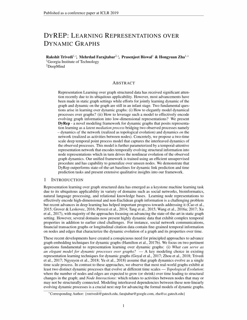
Figure 1: Evolution Through Mediation. (a) Association events (k=0) where the node or edge grows.(c) Communication Events (k=1) where nodes interact with each other. For both these processes,tp,k=0 < (t1, t2, t3, t4, t5)k=1 < tq,k=0 < (t6, t7)k=1 < tr,k=0. (b) Evolving Representations.
(ii) How can one leverage such a model to learn dynamic node representations that are effectivelyable to capture evolving graph information over time? — Existing techniques in this direction can bedivided into two approaches: a.) Discrete-Time Approach, where the evolution of a dynamic graphis observed as collection of static graph snapshots over time (Zhu et al., 2016; Goyal et al., 2017;Zhou et al., 2018). These approaches tend to preserve (encode) very limited structural informationand capture temporal information at a very coarse level which leads to loss of information betweensnapshots and lack of ability to capture fine-grained temporal dynamics. Another challenge insuch approaches is the selection of appropriate aggregation granularity which is often misspecified.b.) Continuous-Time Approach, where evolution is modeled at finer time granularity in order toaddress the above challenges. While existing approaches have demonstrated to be very effective inspecific settings, they either model simple structural and complex temporal properties in a decoupledfashion (Trivedi et al., 2017) or use simple temporal models (exponential family in (Ngyuyen et al.,2018)). But several domains exhibit highly nonlinear evolution of structural properties coupledwith complex temporal dynamics and it remains an open problem to effectively model and learninformative representations capturing various dynamical properties of such complex systems.
As noted in (Chazelle, 2012), an important requirement to effectively learn over such dynamicalsystems is the ability to express the dynamical processes at different scales. We propose that anydynamic graph must be minimally expressed as a result of two fundamental processes evolving atdifferent time scales: Association Process (dynamics of the network), that brings change in thegraph structure and leads to long lasting information exchange between nodes; and CommunicationProcess (dynamics on the network), that relates to activities between (not necessarily connected)nodes which leads to temporary information flow between them (Farine, 2017; Artime et al., 2017).We, then, posit our goal of learning node representations as modeling a latent mediation processthat bridges the above two observed processes such that learned representations drive the complextemporal dynamics of both processes and these processes subsequently lead to the nonlinear evolutionof node representations. Further, the information propagated across the graph is governed by thetemporal dynamics of communication and association histories of nodes with its neighborhood. Forinstance, in a social network, when a node’s neighborhood grows, it changes that node’s representationwhich in turn affects her social interactions (association→ embedding→ communication). Similarly,when node’s interaction behavior changes, it affects the representation of her neighbors and herselfwhich in turn changes the structure and strength of her connections due to link addition or deletion(communication→ embedding→ association). We call this phenomenon — evolution throughmediation and illustrate it graphically in Figure 1.
In this work, we propose a novel representation learning framework for dynamic graphs, DyRep, tomodel interleaved evolution of two observed processes through latent mediation process expressedabove and effectively learn richer node representations over time. Our framework ingests dynamicgraph information in the form of association and communication events over time and updates thenode representations as they appear in these events. We build a two-time scale deep temporal point
2
Published as a conference paper at ICLR 2019
process approach to capture the continuous-time fine-grained temporal dynamics of the two observedprocesses. We further parameterize the conditional intensity function of the temporal point processwith a deep inductive representation network that learns functions to compute node representations.Finally, we couple the structural and temporal components of our framework by designing a novelTemporal Attention Mechanism, which induces temporal attentiveness over neighborhood nodes usingthe learned intensity function. This allows to capture highly interleaved and nonlinear dynamicsgoverning node representations over time. We design an efficient unsupervised training procedure forend-to-end training of our framework. We demonstrate consistent and significant improvement overstate-of-the-art representative baselines on two real-world dynamic graphs for the tasks of dynamiclink prediction and time prediction. We further present an extensive qualitative analysis throughembedding visualization and ablation studies to discern the effectiveness of our framework.
2 BACKGROUND AND PRELIMINARIES
2.1 RELATED WORK
Representation Learning approaches for static graphs either perform node embedding (Cao et al.,2015; Grover & Leskovec, 2016; Perozzi et al., 2014; Tang et al., 2015; Wang et al., 2016a; 2017; Xuet al., 2017) or sub-graph embedding (Scarselli et al., 2009; Li et al., 2016; Dai et al., 2016) which canalso utilize convolutional neural networks (Kipf & Welling, 2017; 2016; Bruna et al., 2014). Amongthem, GraphSage (Hamilton et al., 2017a) is an inductive method for learning functions to computenode representations that can be generalized to unseen nodes. Most of these approaches only workwith static graphs or can model evolving graphs without temporal information. Dynamic networkembedding is pursued through various techniques such as matrix factorization (Zhu et al., 2016),structural properties (Zhou et al., 2018), CNN-based approaches (Seo et al., 2016), deep recurrentmodels (Trivedi et al., 2017), and random walks (Ngyuyen et al., 2018). There exists a rich body ofliterature on temporal modeling of dynamic networks (Kim et al., 2017), that focus on link predictiontasks but their goal is orthogonal to our work as they build task specific methods and do not focuson representation learning. Authors in (Yang et al., 2017; Sarkar et al., 2007) proposed models oflearning dynamic embeddings but none of them consider time at finer level and do not capture bothtopological evolution and interactions simultaneously. In parallel, research on deep point processmodels include parametric approaches to learn intensity (Du et al., 2016; Mei & Eisner, 2017) usingrecurrent neural networks and GAN based approaches to learn intensity functions (Xiao et al., 2017).More detailed related works are provided in Appendix F.
2.2 TEMPORAL POINT PROCESSES
Stochastic point processes (Daley & Vere-Jones, 2007) are random processes whose realizationcomprises of discrete events in time, t1, t2, . . .. A temporal point process is one such stochasticprocess that can be equivalently represented as a counting process, N(t), which contains the numberof events up to time t. The common way to characterize temporal point processes is via the conditionalintensity function λ(t), a stochastic model of rate of happening events given the previous events.Formally, λ(t)dt is the conditional probability of observing an event in the tiny window [t, t+ dt),λ(t)dt := P[event in [t, t+ dt)|T (t)] = E[dN(t)|T (t)], where T (t) = tk|tk < t is history until t.Similarly, for t > tn and given history T = t1, . . . , tn, we characterize the conditional probabilitythat no event happens during [tn, t) as S(t|T ) = exp
(−∫ t
tnλ(τ) dτ
), which is called survival
function of the process (Aalen et al., 2008). Moreover, the conditional density that an event occursat time t is defined as f(t) = λ(t)S(t). The intensity λ(t) is often designed to capture phenomenaof interests – common forms include Poisson Process, Hawkes processes (Farajtabar et al., 2014;Hawkes, 1971; Wang et al., 2016b; Tabibian et al., 2017), Self-Correcting Process (Isham & Westcott,1979). Temporal Point Processes have previously been used to model both – dynamics on thenetwork (Farajtabar et al., 2016; Zarezade et al., 2017; Farajtabar et al., 2017) and dynamics of thenetwork (Tran et al., 2015; Farajtabar et al., 2015).
2.3 NOTATIONS AND DYNAMIC GRAPH SETTING
Notations. Let Gt = (Vt, Et) denote graph G at time t, where Vt is the set of nodes and Et is the set ofedges in Gt and the edges are undirected. Event Observation – Both communication and associationprocesses are realized in the form of dyadic events observed between nodes on graph G over atemporal window [t0, T ] and ordered by time. We use the following canonical tuple representationfor any type of event at time t of the form e = (u, v, t, k), where u, v are the two nodes involved
3
Published as a conference paper at ICLR 2019
in an event. t represents time of the event. k ∈ 0, 1 and we use k = 0 to signify events fromthe topological evolution process (association) and k = 1 to signify events from node interactionprocess (communication). Persistent edges in the graph only appear through topological events whileinteraction events do not contribute them. Hence, k represents an abstraction of scale (evolutionrate) associated with processes that generate topological (dynamic of the network) and interactionevents (dynamic on the network) respectively. We then represent complete set of P observed eventsordered by time in window [0, T ] asO = (u, v, t, k)pPp=1. Here, tp ∈ R+, 0 ≤ tp ≤ T . AppendixB discusses a marked point process view of such an event set. Node Representation— Let zv ∈ Rd
represent d-dimensional representation of node v. As the representation evolve over time, we qualifythem as function of time: zv(t) — the representation of node v being updated after an event involvingv at time t. We use zv(t) for most recently updated embedding of node v just before t.
Dynamic Graph Setting. Let Gt0 = (Vt0 , Et0) be the initial snapshot of a graph at time t0. Pleasenote that Gt0 may be empty or it may contain an initial structure (association edges) but it will nothave any communication history. Our framework observes evolution of graph as a stream of eventsO and hence any new node will always be observed as a part of such an event. This will induce anatural ordering over nodes as available from the data. As our method is inductive, we never learnnode-specific representations and rather learn functions to compute node representations. In thiswork, we only support growth of network i.e. we only model addition of nodes and structural edgesand leave deletion as future work. Further, for general description of the model, we will assume thatan edge in the graph do not have types and nodes do not have attributes but we discuss the details onhow to use our model to accommodate these features in Appendix B.
3 PROPOSED METHOD: DYREP
The key idea of DyRep is to build a unified architecture that can ingest evolving information overgraphs and effectively model the evolution through mediation phenomenon described in Section 1.To achieve this, we design a two-time scale temporal point process model of observed processesand parameterize it with an inductive representation network which subsequently models the latentmediation process of learning node representations. The rationale behind our framework is that theobserved set of events are the realizations of the nonlinear dynamic processes governing the changesin topological structure of graph and interactions between the nodes in the graph. Now, when an eventis observed between two nodes, information flows from the neighborhood of one node to the otherand affects the representations of the nodes accordingly. While a communication event (interaction)only propagates local information across two nodes, an association event changes the topology andthereby has more global effect. The goal is to learn node representations that encode informationevolving due to such local and global effects and further drive the dynamics of the observed events.
3.1 MODELING TWO-TIME SCALE OBSERVED GRAPH DYNAMICS
The observations over dynamic graph contain temporal point patterns of two interleaved complexprocesses in the form of communication and association events respectively. At any time t, theoccurrence of an event, from either of these processes, is dependent on the most recent state of thegraph, i.e., two nodes will participate in any event based on their most current representations. Givenan observed event p = (u, v, t, k), we define a continuous-time deep model of temporal point processusing the conditional intensity function λu,vk (t) that models the occurrence of event p between nodesu and v at time t:
λu,vk (t) = fk(gu,vk (t)) (1)where t signifies the timepoint just before current event. The inner function gk(t) computes thecompatibility of the most recently updated representations of two nodes, zu(t) and zv(t) as follows:
gu,vk (t) = ωTk · [zu(t); zv(t)] (2)
[;] signifies concatenation and ωk ∈ R2d serves as the model parameter that learns time-scale specificcompatibility. gk(t) is a function of node representations learned through a representation networkdescribed in Section 3.2. This network parameterizes the intensity function of the point processmodel which serves as a unifying factor. Note that the dynamics are not two simple point processesdependent on each other, but, they are related through the mediation process and in the embeddingspace. Further, a well curated attention mechanism is employed to learn how the past drives future.
The choice of outer function fk needs to account for two critical criteria: 1) Intensity needs to bepositive. 2) As mentioned before, the dynamics corresponding to communication and association
4
Published as a conference paper at ICLR 2019
processes evolve at different time scales. To account for this, we use a modified version of softplusfunction parameterized by a dynamics parameter ψk to capture this timescale dependence:
fk(x) = ψk log(1 + exp(x/ψk)) (3)
where, x = g(t) in our case and ψk(> 0) is scalar time-scale parameter learned as part of training.ψk corresponds to the rate of events arising from a corresponding process. In 1D event sequences,the formulation in (3) corresponds to the nonlinear transfer function in (Mei & Eisner, 2017).
3.2 LEARNING LATENT MEDIATION PROCESS VIA TEMPORALLY ATTENTIVEREPRESENTATION NETWORK
We build a deep recurrent architecture that parameterizes the intensity function in Eq. (1) andlearns functions to compute node representations. Specifically, after an event has occurred, therepresentation of both the participating nodes need to be updated to capture the effect of the observedevent based on the principles of:
Self-Propagation. Self-propagation can be considered as a minimal component of the dynamicsgoverning an individual node’s evolution. A node evolves in the embedded space with respect to itsprevious position (e.g. set of features) and not in a random fashion.
Exogenous Drive. Some exogenous force may smoothly update the node’s current features duringthe time interval (e.g. between two global events involving that node).
Localized Embedding Propagation. Two nodes involved in an event form a temporary (communica-tion) or a permanent (association) pathway for the information to propagate from the neighborhood ofone node to the other node. This corresponds to the influence of the nodes at second-order proximitypassing through the other node participating in the event (See Appendix A for pictorial depiction).
To realize the above processes in our setting, we first describe an example setup: Consider nodes uand v participating in any type of event at time t. LetNu andNv denote the neighborhood of nodes uand v respectively. We discuss two key points here: 1) Node u serves as a bridge passing informationfrom Nu to node v and hence v receives the information in an aggregated form through u. 2) Whileeach neighbor of u passes its information to v, the information that node u relays is governed by anaggregate function parametrized by u’s communication and association history with its neighbors.
With this setup, for any event at time t, we update the embeddings for both nodes involved in theevent using a recurrent architecture. Specifically, for p-th event of node v, we evolve zv as:
zv(tp) = σ( Wstructhustruct(tp)︸ ︷︷ ︸
Localized Embedding Propagation
+ Wreczv(tvp)︸ ︷︷ ︸Self-Propagation
+ Wt(tp − tvp)︸ ︷︷ ︸Exogenous Drive
), (4)
where, hustruct ∈ Rd is the output representation vectors obtained from aggregator function on node
u’s neighborhood and zv(tvp) is the recurrent state obtained from the previous representation of nodev. tp is time point of current event, tp signifies the timepoint just before current event and tvp representtime point of previous event for node v. zv(tvp = 0), the initial representation of a node v may beinitialized either using input node features from dataset or random vector as per the setting. Eq. 4is a neural network based functional form parameterized by Wstruct,Wrec ∈ Rd×d and Wt ∈ Rd
that govern the aggregate effect of all the three inputs (graph structure, previous embedding andexogenous feature) respectively to compute representations. The above formulation is inductive(supports unseen nodes) and flexible (supports node and edge types) as discussed in Appendix B.
3.2.1 TEMPORALLY ATTENTIVE AGGREGATION
The Localized Embedding Propagation principle above captures rich structural properties based onneighborhood structure which is a key to any representation learning task over graphs. However,for a given node, not all of its neighbors are uniformly important and hence it becomes extremelyimportant to capture information from each neighbor in some weighted fashion. Recently proposedattention mechanisms have shown great success in dealing with variable sized inputs, focusing on themost relevant parts of the input to make decisions. However, existing approaches consider attentionas a static quantity. In dynamic graphs, changing neighborhood structure and interaction activitiesbetween nodes evolves importance of each neighbor to a node over time, thereby making attentionitself a temporally evolving quantity. Further this quantity is dependent on the temporal historyof association and communication of neighboring nodes through evolving representations. To this
5

Published as a conference paper at ICLR 2019
Algorithm 1 Update Algorithm for S and A
Input: Event record o = (u, v, t, k), Event Intensity λu,vk (t) computed in (1), most recentlyupdated A(t) and S(t). Output: A(t) and S(t)
1. Update A : A(t) = A(t)if k = 0 then Auv(t) = Avu(t) = 1 ←Association event
2. Update S : S(t) = S(t)if k = 1 and Auv(t) = 0 return S(t),A(t) ←Communication event, no Association existsfor j ∈ u, v dob = 1
|Nj(t)| where |Nj(t)| is the size of Nj(t) = i : Aij(t) = 1y← Sj(t)if k = 1 and Auv(t) = 1 then ←Communication event, Association exists
yi = b+ λjik (t) where i is the other node involved in the event. ←λ computed in Eq. 2else if k = 0 and Auv(t) = 0 then ←Association eventb′ = 1
|Nj(t)| where |Nj(t)| is the size of Nj(t) = i : Aij(t) = 1x = b′ − byi = b+ λjik (t) where i is the other node involved in the event ←λ computed in Eq. 2yw = yw − x; ∀w 6= i, yw 6= 0
end ifNormalize y and set Sj(t)← y
end forreturn S(t),A(t)
end, we propose a novel Temporal Point Process based Attention Mechanism that uses temporalinformation to compute the attention coefficient for a structural edge between nodes. These coefficientare then used to compute the aggregate quantity (hstruct) required for embedding propagation.
Let A(t) ∈ Rn×n be the adjacency matrix for graph Gt at time t. Let S(t) ∈ Rn×n be a stochasticmatrix capturing the strength between pair of vertices at time t. One can consider S as a selectionmatrix that induces a natural selection process for a node – it would tend to communicate more withother nodes that it wants to associate with or has recently associated with. And it would want toattend less to non-interesting nodes. We start with following implication required for the constructionof hu
struct in (4): For any two nodes u and v at time t, Suv(t) ∈ [0, 1] if Auv(t) = 1 and Suv(t) = 0if Auv(t) = 0. Denote Nu(t) = i : Aiu(t) = 1 as the 1-hop neighborhood of node u at time t.
To formally capture the difference in the influence of different neighbors, we propose anovel conditional intensity based attention layer that uses the matrix S to induce a shared attentionmechanism to compute attention coefficients over neighborhood. Specifically, we perform localizedattention for a given node u and compute the coefficients pertaining to the 1-hop neighbors i of nodeu as: qui(t) = exp(Sui(t))∑
i′∈Nu(t) exp(Sui′ (t)), where qui signifies the attention weight for the neighbor i at
time t and hence it is a temporally evolving quantity. These attention coefficients are then used tocompute the aggregate information hu
struct(t) for node u by employing an attended aggregationmechanism across neighbors as follows: hu
struct(t) = max(σ(qui(t) · hi(t)
),∀i ∈ Nu(t)
),
where, hi(t) = Whzi(t) + bh and Wh ∈ Rd×d and bh ∈ Rd are parameters governing theinformation propagated by each neighbor of u. zi(t) ∈ Rd is the most recent embedding for nodei. The use of max operator is inspired from learning on general point sets (Qi et al., 2017). Byapplying max-pooling operator element-wise, the model effectively captures different aspects of theneighborhood. We found max to work slightly better as it considers temporal aspect of neighborhoodwhich would be amortized if mean is used instead.
Connection to Neural Attention over Graphs. Our proposed temporal attention layer shares themotivation of recently proposed Graph Attention Networks (GAT) (Velickovic et al., 2018) and GatedAttention Networks (GaAN) (Zhang et al., 2018) in the spirit of applying non-uniform attention overneighborhood. Both GAT and GaAN have demonstrated significant success in static graph setting.GAT advances GraphSage (Hamilton et al., 2017a) by employing multi-head non-uniform attention
6
Published as a conference paper at ICLR 2019
over neighborhood and GaAN advances GAT by applying different weights to different heads inthe multi-head attention formulation. The key innovation in our model is the parameterization ofattention mechanism by a point process based temporal quantity S that is evolving and drives theimpact that each neighbor has on the given node. Further, unlike static methods, we use theseattention coefficients as input to the aggregator function for computing the temporal-structural effectof neighborhood. Finally, static methods use multi-head attention to stabilize learning by capturingmultiple representation spaces but this is an inherent property in our layer as representations andevent intensities update over time and hence new events help capture multiple representation spaces.
Construction and Update of S. We construct a single stochastic matrix S (used to parameterizeattention in the earlier section) to capture complex temporal information. At the initial timepointt = t0, we construct S(t0) directly from A(t0). Specifically, for a given node v, we initialize theelements of corresponding row vector Sv(t0) as: Svu(t0) = 0 if (v = u or Avu(t0) = 0) andSvu(t0) = 1
|Nv(t0)| if Nv(t0) = u : Auv(t0) = 1. After observing an event o = (u, v, t, k) attime t > t0, we make updates to A and S as per the observation of k. Specifically, A only getsupdated for association events (k=0, change in structure). Note that S is parameter for a structuraltemporal attention which means temporal attention is only applied on structural neighborhood ofa node. Hence, the values of S are only updated/active in two scenarios: a) the current event isan interaction between nodes which already has structural edge (Auv(t) = 1 and k = 1) and b)the current event is an association event (k = 0). Given a neighborhood of node u, b representsbackground (base) attention for each edge which is uniform attention based on neighborhood size.Whenever an event involving u occurs, this attention changes in following ways: For case (a), theattention value for corresponding S entries are updated using the intensity of the event. For case(b), repeat same as (a) but also adjust the background attention (by b − b′, b and b′ being the newand old background attention respectively) for edge with other neighbors as the neighborhood sizegrows in this case. From mathematical viewpoint, this update resembles a standard temporal pointprocess formulation where the term coming from b serves as background attention while λ can beviewed as endogenous intensity based attention. Algorithm 1 outlines complete update scenarios.In the directed graph case, updates to A will not be symmetric, which will subsequently affect theneighborhood structure and attention flow for a node. Appendix A provides a pictorial depiction ofthe complete DyRep framework discussed in this section. We provide an extensive ablation study inAppendix C that can help discern the contribution of all the above components in achieving our goal.
4 EFFICIENT LEARNING PROCEDURE
The complete parameter space for the current model is Ω = Wstruct,Wrec,Wt,Wh,bh,ωkk=0,1, ψkk=0,1. For a set O of P observed events, we learn these parameters by minimizingthe negative log likelihood: L = −
∑Pp=1 log (λp(t)) +
∫ T
0Λ(τ)dτ , where λp(t) = λ
up,vpkp
(t)
represent the intensity of event at time t and Λ(τ) =∑n
u=1
∑nv=1
∑k∈0,1 λ
u,vk (τ) represent total
survival probability for events that do not happen. While it is intractable (will require O(n2k) time)and unnecessary to compute the integral in the log-likelihood equation for all possible non-events ina stochastic setting, we can locally optimize L using mini-batch stochastic gradient descent where weestimate the integral using novel sampling technique. Algorithm 2 in Appendix H adopts a simplevariant of Monte Carlo trick to compute the survival term of log-likelihood equation. Specifically,in each mini-batch, we sample non-events instead of considering all pairs of non-events (which canbe millions). Let m be the mini-batch size and N be the number of samples. The complexity ofAlgorithm 2 will then be O(2mkN) for the batch where the factor of 2 accounts for the updatehappening for two nodes per event which demonstrates linear scalability in number of events which isdesired to tackle web-scale dynamic networks (Paranjape et al., 2017). The overall training procedureis adopted from (Trivedi et al., 2017) where the Backpropagation Through Time (BPTT) trainingis conducted over a global sequence, thereby maintaining the dependencies between events acrosssequences while avoiding gradient related issues. Implementation details are left to Appendix G.
5 EXPERIMENTS
5.1 DATASETS
We evaluate DyRep and baselines on two real world datasets: Social Evolution Dataset releasedby MIT Human Dynamics Lab — #nodes: 83, #Initial Associations: 376, #Final Associations:791, #Communications: 2016339 and Clustering Coefficient: 0.548. Github Dataset availableat Github Archive — #nodes: 12328, #Initial Associations: 70640, #Final Associations: 166565,
7
Published as a conference paper at ICLR 2019
Table 1: Comparison of DyRep with state-of-the-art approaches
Key DyRep Know-Evolve DynGem GraphSage GATProperties (Our Method) (Dynamic) (Dynamic) (Static) (Static)
Models Association X X X X XModels Communication X X X X X
Models Time X X X X XLearns Representation X X X X X
Predicts Time X X X X XGraph Information 2nd-order Single 1st and 2nd-order 2nd-order 1st-order
Neighborhood Edge Neighborhood Neighborhood NeighborhoodAttention Mechanism Temporal Point Process None None Sampling Multi-head
(Non-Uniform) (Uniform) (Non-Uniform)Learning Unsupervised Unsupervised Semi-Supervised Unsupervised Supervised
#Communications: 604649 and Clustering Coefficient: 0.087. These datasets cover a range ofconfigurations as Social Dataset is a small network with high clustering coefficient and over 2Mevents. In contrast, Github dataset forms a large network with low clustering coefficient and sparseevents thus allowing us to test the robustness of our model. Further, Github dataset contains severalunseen nodes which were never encountered during training.
5.2 TASKS AND METRICS
We study the effectiveness of DyRep by evaluating our model on tasks of dynamic link predictionand event time prediction tasks:
Dynamic Link Prediction. When any two nodes in a graph has increased rate of interaction events,they are more likely to get involved in further interactions and eventually these interactions may leadto the formation of structural link between them. Similarly, formation of the structural link may leadto increased likelihood of interactions between newly connected nodes. To understand, how well ourmodel captures these phenomenon, we ask questions like: Which is the most likely node u that wouldundergo an event with a given node v governed by dynamics k at time t? The conditional densityof such and event at time t can be computed: fu,vk (t) = λu,vk (t) · exp
(∫ t
tλ(s)ds
), where t is the
time of the most recent event on either dimension u or v. We use this conditional density to find mostlikely node.
For a given test record (u, v, t, k), we replace v with other entities in the graph and compute thedensity as above. We then rank all the entities in descending order of the density and report the rankof the ground truth entity. Please note that the latest embeddings of the nodes update even during thetest while the parameters of the model remaining fixed. Hence, when ranking the entities, we removeany entities that creates a pair already seen in the test. We report Mean Average Rank (MAR) andHITS(@10) metric for dynamic link prediction.
Event Time Prediction. This is a relatively novel application where the aim is to compute the nexttime point when a particular type of event (structural or interaction) can occur. Given a pair of nodes(u, v) and event type k at time t, we use the above density formulation to compute conditional densityat time t. The next time point t for the event can then be computed as: t =
∫∞ttfu,vk (t)dt where the
integral does not have an analytic form and hence we estimate it using Monte Carlo trick. For a giventest record (u, v, t, k), we compute the next time this communication event may occur and reportMean Absolute Error (MAE) against the ground truth.
5.3 BASELINES
Dynamic Link Prediction. We compare the performance of our model against multiple represen-tation learning baselines, four of which has capability to model evolving graphs. Specifically, wecompare with Know-Evolve (Trivedi et al., 2017)— a state-of-the-art model for multi-relationaldynamic graphs where each edge has time-stamp and type (communication events), DynGem (Goyalet al., 2017)—divides timeline into discrete time points and learns embedding for the graph snapshotsat these time points. DynTrd (Zhou et al., 2018) focuses on specific structure of triad to modelhow close triads are formed from open triads in dynamic networks. GraphSage (Hamilton et al.,2017a)— an inductive representation learning method that learns sample and aggregation functionsto learn representations instead of training for individual node. Node2Vec (Grover & Leskovec,2016)—simple transductive baseline to learn graph embeddings over static graphs. Table 1 providesqualitative comparison between state-of-the-art methods and our framework. In our experiments, wecompare with GraphSage instead of GAT as we share the unsupervised setting with GraphSage while
8

Published as a conference paper at ICLR 2019
0
20
40
60
1 2 3 4 5 6Time_Slot
MAR
DynGemDynTrd
DyRepGraphSage
Know-EvolveNode2Vec
11.077313.4774
42.5548 42.74
19.0348
40.5741
0
10
20
30
40
50
Methods
MAR
DyRepKnow-Evolve
DynGemDynTrd
GraphSageNode2Vec
3500
4000
4500
1 2 3 4 5 6Time_Slot
MAR
DynGemDynTrd
DyRepGraphSage
Know-EvolveNode2Vec
2722.813007.0233
3762.024
4149.9546
3124.5371
4202.606
0
1000
2000
3000
4000
Methods
MAR
DyRepKnow-Evolve
DynGemDynTrd
GraphSageNode2Vec
(a) Social (Communication) (b) Social (Association) (c) Github (Communication) (c) Github (Association)
Figure 2: Dynamic Link Prediction Performance for (a-b) Social Evolution Dataset (c-d) GithubDataset. We report HITS@10 results and zoomed versions in Appendix E. Best viewed in pdf.
GAT is designed for supervised learning. In Appendix A (Ablation studies), we show results on oneversion where we only update attention based on Association events which is temporal analogous toGAT.
Event Time Prediction. We compare our model against (i) Know-Evolve which has the ability topredict time in a multi-relational dynamic graphs (II) Multi-dimensional Hawkes Process (MHP) (Duet al., 2015) model where all events in graph are considered as dyadic.
5.4 EVALUATION SCHEME
We divide our test sets into n(= 6) slots based on time and report the performance for each time slot,thus providing comprehensive temporal evaluation of different methods. This method of reporting isexpected to provide fine-grained insights on how various methods perform over time as they movefarther from the learned training history. For dynamic baselines that do not explicitly model time(DynGem, DynTrd, GraphSage) and static baselines (Node2Vec), we adopt a sliding window trainingapproach with warm-start method where we learn on initial train set and test for the first slot. Thenwe add the data from first slot in the train set and remove equal amount of data from start of train setand retrain the model using the embeddings from previous train.
5.5 EXPERIMENTAL RESULTS
Communication Event Prediction Performance. We first consider the task of predicting commu-nication events between nodes which may or may not have a permanent edge (association) betweenthem. Figure 2 (a-b) shows corresponding results.
Social Evolution. Our method significantly and consistently outperforms all the baselines onboth metrics. While the performance of our method drops a little over time, it is expected dueto the temporal recency affect on node’s evolution. Know-Evolve can capture event dynamicswell and shows consistently better rank than others but its performance deteriorates significantlyin HITS@10 metric over time. We conjecture that features learned through edge-level modelinglimits the predictive capacity of the method over time. The inability of DynGem (snapshot baseddynamic), DynTrd and GraphSage (inductive) to significantly outperform Node2vec (transductivestatic baseline) demonstrate that discrete time snapshot based models fail to capture fine-graineddynamics of communication events.
Github dataset. We demonstrate comparable performance with both Know-Evolve and GraphSageon Rank metric. We would like to note that overall performance for all methods on rank metricis low. As we reported earlier, Github dataset is very sparse with very low clustering coefficientwhich makes it a challenging dataset to learn. It is expected that for a large number of nodes withno communication history, most of the methods will show comparable performance but our methodoutperforms all others when there is some history available. This is demonstrated by our significantlybetter performance for HITS@10 metric where we are able to do highly accurate prediction for nodeswhere we learn better history. This can also be attributed to our model’s ability to capture the effectof evolving topology which is missed by Know-Evolve. Finally, we do not see significant decrease inperformance of any method over time in this case which can again be attributed to roughly uniformdistribution of nodes with no communication history across time slots.
Association Event Prediction Performance. Association events are not available for all time slotsso Figure 2 (c-d) report the aggregate number for this task. For both the datasets, our modelsignificantly outperforms the baselines for this task. Specifically, our model’s strong performance onHITS@10 metric across both datasets demonstrates its robustness in accurate learning from variousproperties of data. On Social evolution dataset, the number of association events are very small(only 485) and hence our strong performance shows that the model is able to capture the influence
9
Published as a conference paper at ICLR 2019
0
500
1000
1500
1 2 3 4 5 6Time_Slot
MAE
DyRep Know-Evolve MHP
0
500
1000
1500
2000
2500
1 2 3 4 5 6Time_Slot
MAE
DyRep Know-Evolve MHP
23.4448129.2163
1179.6804
0
500
1000
1500
Methods
MAE
MethodDyRepKnow-EvolveMHP
110.3168301.4191
1917.2893
0
500
1000
1500
2000
Methods
MAE
MethodDyRepKnow-EvolveMHP
(a) Social Evolution (b) Github (c) Social Evolution (d) Github
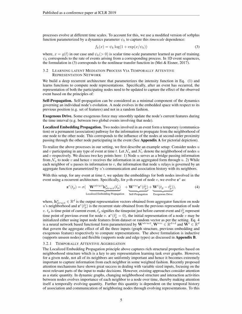
Figure 3: Time Prediction Performance (unit is hrs). Figure best viewed in pdf or colored print.
100 75 50 25 0 25 50 75100
75
50
25
0
25
50
75
100
100 75 50 25 0 25 50 75
75
50
25
0
25
50
75
20 10 0 10 20
10
0
10
20
1926
20 10 0 10 20
20
15
10
5
0
5
10
1519
26
(a) DyRep Embeddings (b) GraphSage Embeddings (c) DyRep Embeddings (d) GraphSage Embeddings
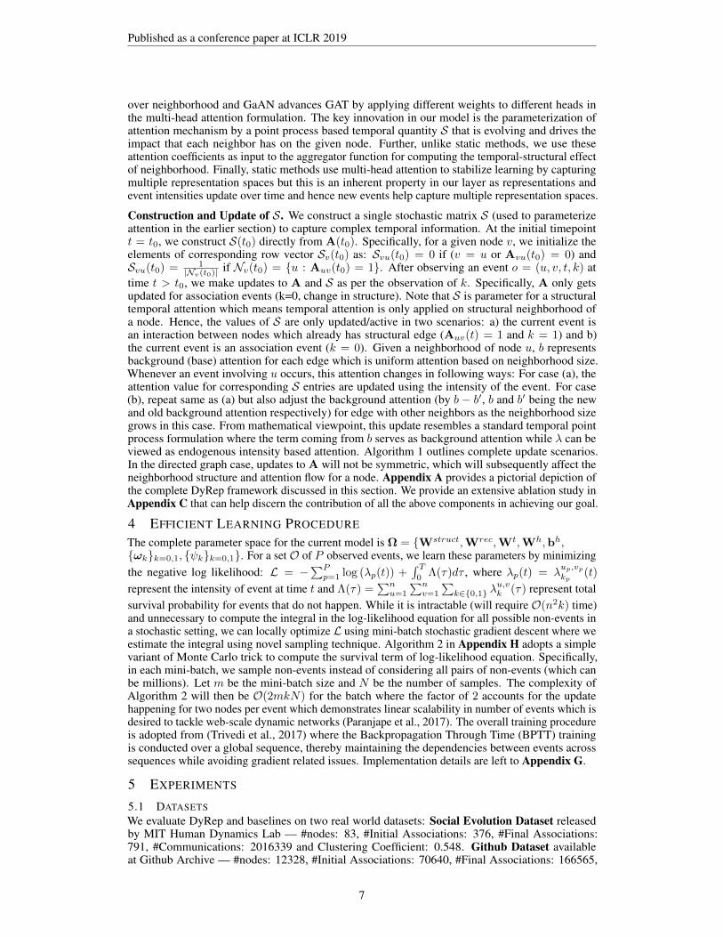
Figure 4: tSNE for learned embeddings after training. Figure best viewed in color.of communication events on the association events through the learned representations (mediation).On the Github dataset, the network grows through new nodes and our model’s strong performanceacross both metric demonstrates its inductive ability to generalize across new nodes across time. Aninteresting observation was poor performance of DynTrd which seems to be due to its objective tocomplete triangles. Github dataset is very sparse and has very few possibilities for triadic closure.
Time Prediction Performance. Figure 3 demonstrates consistently better performance than state-of-the-art baseline for event time prediction on both datasets. While Know-Evolve models bothprocesses as two different relations between entities, it does not explicitly capture the variance in thetime scales of two processes. Further, Know-Evolve does not consider influence of neighborhoodwhich may lead to capturing weaker temporal-structural dynamics across the graph. MHP usesspecific parametric intensity function which fails to account for intricate dependencies across graph.
Qualitative Performance. We conducted a series of qualitative analysis to understand the discrim-inative power of evolving embeddings learned by DyRep. We compare our embeddings againstGraphSage embeddings as it is state-of-the-art embedding method that is also inductive. Figure 4(a-b) shows the tSNE embeddings learned by Dyrep (left) and GraphSage (right) respectively. Thevisualization demonstrates that DyRep embeddings have more discriminative power as it can effec-tively capture the distinctive and evolving structural features over time as aligned with empiricalevidence. Figure 4 (c-d) shows use case of two associated nodes (19 and 26) that has persistent edgebut less communication for above two methods. DyRep keeps the embeddings nearby although notin same cluster (cos. dist. - 0.649) which demonstrates its ability to learn the association and lesscommunication dynamics between two nodes. For GraphSage the embeddings are on opposite endsof cluster with (cos. dist. - 1.964). We provide more extensive analysis in Appendix D.
6 CONCLUSION
We introduced a novel modeling framework for dynamic graphs that effectively and efficiently learnsnode representations by posing representation learning as latent mediation process bridging dynamicprocesses of topological evolution and node interactions. We proposed a deep temporal point processmodel parameterized by temporally attentive representation network that models these complex andnonlinearly evolving dynamic processes and learns to encode structural-temporal information overgraph into low dimensional representations. Our superior evaluation performance demonstrates theeffectiveness of our approach compared to state-of-the-art methods. We present this work as thefirst generic and unified representation learning framework that adopts a novel modeling paradigmfor dynamic graphs and support wide range of dynamic graph characteristics which can potentiallyhave many exciting adaptations. As a part of our framework, we also propose a novel temporalpoint process based attention mechanism that can attend over neighborhood based on the history ofcommunications and association events in the graph. Currently, DyRep does not support networkshrinkage due to following reasons: (i) It is difficult to procure data with fine grained deletion timestamps and (ii) The temporal point process model requires more sophistication to support deletion.For example, one can augment the model with a survival process formulation to account for lack ofnode/edge at future time. Another interesting future direction could be to support encoding higherorder dynamic structures.
10

Published as a conference paper at ICLR 2019
ACKNOWLEDGEMENTS
We sincerely thank our anonymous ICLR reviewers for critical feedback that helped us to improvethe clarity and precision of our presentation. We would also like to thank Jiachen Yang (GeorgiaTech) for insightful comments on improving the presentation of the paper. This work was supportedin part by NSF IIS-1717916, NSF CMMI-1745382, NSFC-Zhejiang Joint Fund for the Integration ofIndustrialization and Information (U1609220) and National Science Foundation of China (61672231).
REFERENCES
Odd Aalen, Ornulf Borgan, and Hakon Gjessing. Survival and event history analysis: a process pointof view. 2008.
Oriol Artime, Jose J. Ramasco, and Maxi San Miguel. Dynamics on networks: competition oftemporal and topological correlations. arXiv:1604.04155, 2017.
Robert Bamler and Stephan Mandt. Dynamic word embedding. In ICML, 2017.
Joan Bruna, Wojciech Zaremba, Arthur Szlam, and Yann LeCun. Spectral networks and locallyconnected networks on graphs. In ICLR, 2014.
Shaosheng Cao, Wei Lu, and Qiongkai Xu. Grarep: Learning graph representations with globalstructural information. In CIKM, 2015.
Bernard Chazelle. Natural algorithms and influence systems. Communications of the ACM, 2012.
Hanjun Dai, Bo Dai, and Le Song. Discriminative embeddings of latent variable models for structureddata. In ICML, 2016.
DJ Daley and D Vere-Jones. An Introduction to the Theory of Point Processes: Volume I: ElementaryTheory and Methods. 2007.
Nan Du, Yichen Wang, Niao He, and Le Song. Time sensitive recommendation from recurrent useractivities. In NIPS, 2015.
Nan Du, Hanjun Dai, Rakshit Trivedi, Utkarsh Upadhyay, Manuel Gomez-Rodriguez, and Le Song.Recurrent marked temporal point processes: Embedding event history to vector. In KDD, 2016.
Cristobal Esteban, Volker Tresp, Yinchong Yang, Stephan Baier, and Denis Krompa. Predicting theco-evolution of event and knowledge graphs. In FUSION, 2016.
Mehrdad Farajtabar, Nan Du, Manuel Gomez Rodriguez, Isabel Valera, Hongyuan Zha, and Le Song.Shaping social activity by incentivizing users. In NIPS, 2014.
Mehrdad Farajtabar, Yichen Wang, Manuel Gomez-Rodriguez, Shuang Li, Hongyuan Zha, andLe Song. Coevolve: A joint point process model for information diffusion and network co-evolution. In NIPS, 2015.
Mehrdad Farajtabar, Xiaojing Ye, Sahar Harati, Le Song, and Hongyuan Zha. Multistage campaigningin social networks. In NIPS, 2016.
Mehrdad Farajtabar, Jiachen Yang, Xiaojing Ye, Huan Xu, Rakshit Trivedi, Elias Khalil, Shuang Li,Le Song, and Hongyuan Zha. Fake news mitigation via point process based intervention. In ICML,2017.
Damien Farine. The dynamics of transmission and the dynamics of networks. Journal of AnimalEcology, 86(3):415–418, 2017.
Palash Goyal, Nitin Kamra, Xinran He, and Yan Liu. Dyngem: Deep embedding method for dynamicgraphs. IJCAI International Workshop on Representation Learning for Graphs, 2017.
Aditya Grover and Jure Leskovec. node2vec: Scalable feature learning for networks. In KDD, 2016.
11
Published as a conference paper at ICLR 2019
William L Hamilton, Rex Ying, and Jure Leskovec. Inductive representation learning on large graphs.In NIPS, 2017a.
William L. Hamilton, Rex Ying, and Jure Leskovec. Representation learning on graphs: Methodsand applications. arXiv:1709.05584, 2017b.
Alan G Hawkes. Spectra of some self-exciting and mutually exciting point processes. Biometrika, 58(1):83–90, 1971.
V. Isham and M. Westcott. A self-correcting point process. Advances in Applied Probability, 37:629–646, 1979.
Ghassen Jerfel, Mehmet E. Basbug, and Barbara E. Engelhardt. Dynamic collaborative filtering withcompund poisson factorization. In AISTATS, 2017.
Tingsong Jiang, Tianyu Liu, Tao Ge, Lei Sha, Sujian Li, Baobao Chang, and Zhifang Sui. Encodingtemporal information for time-aware link prediction. In ACL, 2016.
Bomin Kim, Kevin Lee, Lingzhou Xue, and Xiaoyue Niu. A review of dynamic network modelswith latent variables. arXiv:1711.10421, 2017.
Thomas N Kipf and Max Welling. Variational graph auto-encoders. arXiv:1611.07308, 2016.
Thomas N Kipf and Max Welling. Semi-supervised classification with graph convolutional networks.In ICLR, 2017.
Jundong Li, Harsh Dani, Xia Hu, Jilaing Tang, Yi Change, and Huan Liu. Attributed networkembedding for learning in a dynamic environment. In CIKM, 2017.
Yujia Li, Daniel Tarlow, Marc Brockschmidt, and Richard Zemel. Gated graph sequence neuralnetworks. In ICLR, 2016.
Corrado Loglisci and Donato Malerba. Leveraging temporal autocorrelation of historical data forimproving accuracy in network regression. Statistical Analysis and Data Mining: The ASA DataScience Journal, 2017.
Corrado Loglisci, Michelangelo Ceci, and Donato Malerba. Relational mining for discoveringchanges in evolving networks. Neurocomputing, 2015.
Hongyuan Mei and Jason M Eisner. The neural hawkes process: A neurally self-modulatingmultivariate point process. In NIPS, 2017.
Changpin Meng, Chandra S. Mouli, Bruno Ribeiro, and Jennifer Neville. Subgraph pattern neuralnetworks for high-order graph evolution prediction. In AAAI, 2018.
Giang Hoang Ngyuyen, John Boaz Lee, Ryan A. Rossi, Nesreen K. Ahmed, Eunyee Koh, andSungchul Kim. Continuous-time dynamic network embeddings. In WWW, 2018.
Ashwin Paranjape, Austin R. Benson, and Jure Leskovec. Motifs in temporal networks. In WSDM,2017.
Bryan Perozzi, Rami Al-Rfou, and Steven Skiena. Deepwalk: Online learning of social representa-tions. In KDD, 2014.
Charles R. Qi, Hao Su, Kaichun Mo, and Leonidas J. Guibas. Pointnet: Deep learning on point setsfor 3d classification and segmentation. In CVPR, 2017.
Maja Rudolph and David Blei. Dynamic embeddings for language evolution. In WWW, 2018.
Purnamrita Sarkar, Sajid Siddiqi, and Geoffrey Gordon. A latent space approach to dynamicembedding of co-occurence data. In AISTATS, 2007.
Franco Scarselli, Marco Gori, Ah Chung Tsoi, Markus Hagenbuchner, and Gabriele Monfardini. Thegraph neural network model. Neural Networks, IEEE Transactions on, 20(1):61–80, 2009.
12
Published as a conference paper at ICLR 2019
Youngjoo Seo, Michael Defferrard, Pierre Vandergheynst, and Xavier Bresson. Structured sequencemodeling with graph convolutional recurrent networks. arXiv:1612.07659, 2016.
Behzad Tabibian, Isabel Valera, Mehrdad Farajtabar, Le Song, Bernhard Schölkopf, and ManuelGomez-Rodriguez. Distilling information reliability and source trustworthiness from digital traces.In WWW, 2017.
Jian Tang, Meng Qu, Mingzhe Wang, Ming Zhang, Jun Yan, and Qiaozhu Mei. Line: Large-scaleinformation network embedding. In WWW, 2015.
Long Tran, Mehrdad Farajtabar, Le Song, and Hongyuan Zha. Netcodec: Community detection fromindividual activities. In SDM, 2015.
Rakshit Trivedi, Hanjun Dai, Yichen Wang, and Le Song. Know-evolve: Deep temporal reasoningfor dynamic knowledge graphs. In ICML, 2017.
Petar Velickovic, Guillem Cucurull, Arantxa Casanova, Adriana Romero, Pietro Liò, and YoshuaBengio. Graph attention networks. In ICLR, 2018.
Daixin Wang, Peng Cui, and Wenwu Zhu. Structural deep network embedding. In KDD, 2016a.
Xiao Wang, Peng Cui, Jing Wang, Jian Pei, Wenwu Zhu, and Shiquiang Yang. Community preservingnetwork embedding. In AAAI, 2017.
Yichen Wang, Bo Xie, Nan Du, and Le Song. Isotonic hawkes processes. In ICML, 2016b.
Shuai Xiao, Mehrdad Farajtabar, Xiaojing Ye, Junchi Yan, Le Song, and Hongyuan Zha. Wassersteinlearning of deep generative point process models. In NIPS, 2017.
Linchuan Xu, Xiaokai Wei, Jiannong Cao, and Philip Y. Yu. Embedding identity and interest forsocial networks. In WWW, 2017.
Carl Yang, Mengxiong Liu, Zongyi Wang, Liuyan Liu, and Jiawei Han. Graph clustering withdynamic embedding. arXiv:1712.08249, 2017.
Wenchao Yu, Wei Cheng, Charu C. Aggarwal, Kai Zhang, Haifeng Chen, and Wei Wang. Netwalk:A flexible deep embedding approach for anamoly detection in dynamic networks. In KDD, 2018.
Yuan Yuan, Xiaodan Liang, Xiaolong Wang, Dit-Yan Yeung, and Abhinav Gupta. Temporal dynamicgraph lstm for action-driven video object detection. In ICCV, 2017.
Ali Zarezade, Ali Khodadadi, Mehrdad Farajtabar, Hamid R Rabiee, and Hongyuan Zha. Correlatedcascades: Compete or cooperate. In AAAI, 2017.
Jiani Zhang, Xingjian Shi, Junyuan Xie, hao Ma, Irwin King, and Dit-Yan Yeung. Gaan: Gatedattention networks for learning on large spatiotemporal graphs. In UAI, 2018.
Lekui Zhou, Yang Yang, Xiang Ren, Fei Wu, and Yueting Zhuang. Dynamic network embedding bymodeling triadic closure process. In AAAI, 2018.
Linhong Zhu, dong Guo, Junming Yin, Greg Ver Steeg, and Aram Galstyan. Scalable temporal latentspace inference for link prediction in dynamic social networks. TKDE, 2016.
Yuan Zuo, Guannan Liu, Hao Lin, Jia Guo, Xiaoqian Hu, and Junjie Wu. Embedding temporalnetwork via neighborhood formation. In KDD, 2018.
13

Published as a conference paper at ICLR 2019
APPENDIX
A PICTORIAL EXPOSITION OF DYREP REPRESENTATION NETWORK
A.1 LOCALIZED EMBEDDING PROPAGATION
u v
1
4
3
2 5
6
7
𝒛"()
𝒛'()
𝒛(()
𝒛)()
𝒛*()
𝒛+()
𝒛,()
𝒛-()
𝒛.()
𝒉012*31. ()
𝒉012*31* ()
Figure 5: Localized Embedding Propagation: An event is observed between nodes u and v andk can be 0 or 1 i.e. It can either be a topological event or interaction event. The first term in Eq 4.contains hstruct which is computed for updating each node involved in the event. For node u, theupdate will come from hv
struct (green flow) and for node v, the update will come from hustruct (red
flow). Please note all embeddings are dynamically evolving hence the information flow after everyevent is different and evolves in a complex fashion. With this mechanism, the information is passedfrom neighbors of node u to node v and neighbors of node v to node u. (i) Interaction events lead totemporary pathway - such events can occur between nodes which are not connected. In that case,this flow will occur only once but it will not make u and v neighbors of each other (e.g. meetingat a conference). (ii) Topological events lead to permanent pathway - in this case u and v becomesneighbor of each other and hence will contribute to structural properties moving forward (e.g. beingacademic friends). The difference in number of blue arrows on each side signify different importanceof each node to node u and node v respectively.
Overall Embedding Update Process. As a starting point, neighborhood only includes nodesconnected by a structural edge. On observing an event, we update the embeddings of two nodesinvolved in the event using Eq 4. For a node u, the first term of Eq 4 (Localized EmbeddingPropagation) requires hstruct which is the information that is passed from neighborhood (Nv) ofnode v to node u via node v (one can visualize v as being the message passer from its neighborhoodto u). This information is used to update the embedding of node u. However, we posit that node vdoes not relay equal amount of information from its neighbors to node u. Rather, node v receivesits information to be relayed based on its communication and association history with its neighbors(which relates to importance of each neighbor). This requires to compute the attention coefficientson the structural edges between node v and its neighbors. For any edge, we want this coefficient tobe dependent on rate of events between the two nodes (thereby emulating real world phenomenonthat one gains more information from people one interacts more with). Hence, we parameterize ourattention module with the temporal point process parameter Suv . Algorithm 1 outlines the process ofcomputing the value of this parameter.
14

Published as a conference paper at ICLR 2019
A.2 COMPUTING hstruct: TEMPORAL POINT PROCESS BASED ATTENTION
u v
1
4
3
2
𝒛"()
𝒛'()
𝒛(()
𝒛)()
𝒛*()
𝒉,-.*/-* ()
𝑞*(() 𝑞*)()
𝑞*'()
Temporal Point Process Self-Attention:
𝒉,-.*/-* = max( 𝜎(𝑞*6 ∗ 𝒉6 ) )
𝒉6 = 𝑾9𝒛6 +𝑏9
where 𝑖 ∈ 𝑁* is the node in neighborhood of node u.
𝑞*6
= exp(𝑆*6())
∑ exp(𝑆*6D ())6D ∈EF -
𝒛G()
Figure 6: Temporal Point Process based Self-Attention: This figure illustrates the computation ofhustruct for node u to pass to node v for the same event described before between nodes u and v
at time t with any k. hustruct is computed by aggregating information from neighbors (1,2,3) of
u. However, Nodes that are closely connected or has higher interactions tend to attend more toeach other compared to nodes that are not connected or nodes between which interactions is lesseven in presence of connection. Further, every node has a specific attention span for other nodeand therefore attention itself is a temporally evolving quantity. DyRep computes the temporallyevolving attention based on association and communication history between connected nodes. Theattention coefficient function (q’s) is parameterized by S which is computed using the intensity ofevents between connected nodes. Such attention mechanism allows the evolution of importance ofneighbors to a particular node (u in this case) which aligns with real-world phenomenon.
A.3 COMPUTING S : ALGORITHM 1
Please check Figure 7 on next page.
B RATIONALE BEHIND DYREP FRAMEWORK
Connection to Marked Point Process. From a mathematical viewpoint, for any event e at time t,any information other than the time point can be considered a part of mark space describing the events.Hence, for DyRep, given a one-dimensional timeline, one can consider O = (u, v, k)p, tp)Pp=1 as amarked process with the triple (u, v, k) representing the mark.
However, from machine learning perspective, using a single-dimensional process with suchmarks does not allow to efficiently and effectively discover or model the structure in the point processuseful for learning intricate dependencies between events, participants of the events and dynamicsgoverning those events. Hence, it is often important to extract the information out of the mark spaceand build an abstraction that helps to discover the structure in point process and make this learningparameter efficient. In our case, this translates to two components:
1. The nodes in the graph are considered as dimensions of the point process, thus making it amulti-dimensional point process where an event represents interaction/structure between thedimensions, thus allowing us to explicitly capture dependencies between nodes.
2. The topological evolution of networks happen at much different temporal scale than activitieson a fixed topology network (e.g. rate of making friends vs liking a post on a social network).However both these processes affect each other’s evolution in a complex and nonlinear
15
Published as a conference paper at ICLR 2019
u
1
4
3
2
𝒛"()
𝒛'()
𝒛(()
𝒛)()
𝒛*()
5
𝒛+()
𝑆*( 𝑡 = b = 0.25
𝑆*'(𝑡) = b = 0.25 𝑆*3(𝑡) = b = 0.25
𝑆*)(𝑡) = b = 0.25
𝑆'"(𝑡) = b = 1
(a) Start State
u
1
4
3
2
𝒛"()
𝒛'()
𝒛(()
𝒛)()
𝒛*()
5
𝒛+()
𝑆*( 𝑡 = 0.25
𝑆*'(𝑡) = 0.25𝑆*2(𝑡) = 0.25+ 𝜆56)*2 (𝑡)
𝑆*)(𝑡) = 0.25
𝑆'"(𝑡) = 1𝜆56)*2 (𝑡)
Interaction Event on an existing edge(Note b = 0.25 previously)
u
1
4
3
2
𝒛"()
𝒛'()
𝒛(()
𝒛)()
𝒛*()
5
𝒛+()
𝑆*( 𝑡 = 𝑆*( 𝑡 − 𝑥
𝑆*'(𝑡) = 𝑆*' 𝑡 − 𝑥 𝑆*0(𝑡) = 𝑆*0 𝑡 − 𝑥
𝑆*)(𝑡) = 𝑆*) 𝑡 − 𝑥
𝑆'"(𝑡) = 1 𝑆*"(𝑡) = 𝑏 + 𝜆56)*" (𝑡) Topological Event on a
non-existing edge(Note 𝑏 = 0.2 now and 𝑥 = 𝑏’(𝑝𝑟𝑒𝑣𝑖𝑜𝑢𝑠𝑏)−𝑏 = 0.25– 0.2 = 0.5)
𝜆56)*" (𝑡)
Adjustment due to growth in neighborhood size
(b) Update to S after Interaction Event (c) Update to S after Topological Event
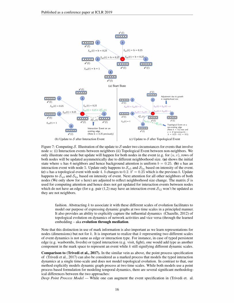
Figure 7: Computing S . Illustration of the update to S under two circumstances for events that involvenode u: (i) Interaction events between neighbors (ii) Topological Event between non-neighbors. Weonly illustrate one node but update will happen for both nodes in the event (e.g. for (u, v), rows ofboth nodes will be updated asymmetrically due to different neighborhood size. (a) shows the initialstate where u has 4 neighbors and hence background attention is uniform b = 0.25. (b) u has aninteraction event with node 5. Update only happens to Su5 and S5u based on intensity of the event.(c) u has a topological event with node 4. b changes to 0.2. b′ = 0.25 which is the previous b. Updatehappens to Su4 and S4u based on intensity of event. Next attention for all other neighbors of bothnodes (We only show for u here) are adjusted to reflect neighborhood size change. The matrix S isused for computing attention and hence does not get updated for interaction events between nodeswhich do not have an edge (for e.g. pair (1,2) may have an interaction event S12 won’t be updated asthey are not neighbors.
fashion. Abstracting k to associate it with these different scales of evolution facilitates tomodel our purpose of expressing dynamic graphs at two time scales in a principled manner.It also provides an ability to explicitly capture the influential dynamics (Chazelle, 2012) oftopological evolution on dynamics of network activities and vice versa (through the learnedembedding – aka evolution through mediation.
Note that this distinction in use of mark information is also important as we learn representations fornodes (dimensions) but not for k. It is important to realize that k representing two different scalesof event dynamics is not same as edge or interaction type. For instance, in case of typed persistentedge (e.g. wasbornIn, livesIn) or typed interaction (e.g. visit, fight), one would add type as anothercomponent in the mark space to represent an event while k still signifying different dynamic scales.
Comparison to (Trivedi et al., 2017). In the similar vein as above, the point process specificationof (Trivedi et al., 2017) can also be considered as a marked process that models the typed interactiondynamics at a single time-scale and does not model topological evolution. In contrast to that, ourmethod explicitly models dynamic graph process at two time scales. While both models use a pointprocess based formulation for modeling temporal dynamics, there are several significant methodolog-ical differences between the two approaches:Deep Point Process Model — While one can augment the event specification in (Trivedi et. al.
16
Published as a conference paper at ICLR 2019
2017) with additional mark information, that itself is not adequate to achieve DyRep’s modelingof dynamical process over graphs at multiple time scales. We employ a softplus function for fkwhich contains a dynamic specific scale parameter ψk to achieve this while (Trivedi et al. 2017) usesan exponential (exp) function for f with no scale parameter. Their intensity formulation attains aRayleigh distribution which leads to a specific assumption about underlying dynamics which modelsfads where intensity of events drop rapidly between events after increasing. Our two-time scalemodel is more general and induces modularization, where each of two components allow complex,nonlinear and dependent dynamics towards a non-zero steady state intensity.Graph Structure— As shown in (Hamilton et al., 2017b), the key idea behind representation learningover graphs is to capture both the global position and local neighborhood structural information ofnode into its representations. Hence, there has been significant research efforts invested in devisingmethods to incorporate graph structure into the computation of node representation. Aligned withthese efforts, DyRep proposes a novel and sophisticated Localized Embedding Propagation principlethat dynamically incorporates graph structure from both local neighborhood and faraway nodes (asinteractions are allowed between nodes that do not have an edge). Contrary to that, (Trivedi et al.,2017) uses single edge level information, specific to the relational setting, into their representations.Deep Temporal Point Process Based Self-Attention— For learning over graphs, attention has beenshown to be extremely valuable as importance of nodes differ significantly relative to each other.The state-of-the-art approaches have focused solely on static graphs with Graph Attention Net-works (Velickovic et al., 2018) being the most recent one. Our attention mechanism for dynamicgraphs present a significant and principled advancement over the existing state-of-the-art Graph basedNeural Self-Attention techniques which only support static graphs. As (Trivedi et al., 2017) do notincorporate graph structure, they do not use any kind of attention mechanism.
Support for Node Attributes and Edge Types. Node types or attributes are supported in our work.In Eq. 4, zv(tp
v) induces recurrence on node v’s embedding, but when node v is observed for first
time, zv(tpv) = xv where xv is randomly initialized or contains the raw node features available in
data (which also includes type). One can also add an extra term in Eq. 4 to support high-dimensionnode attributes. Further, we also support different types of edges. If either the structural edge or aninteraction has a type associated with it, our model can trivially support it in Eq. 3 and Eq. 4, firstterm hstruct. Currently, for computing hstruct, the formulation is shown to use aggregation overnodes. However, this aggregation can be augmented with edge type information as conventionallydone in many representation learning frameworks (Hamilton et al., 2017b). Further, for more directeffect, Eq 3 can include edge type as third feature vector in the concatenation for computing gk.
Support for new nodes. As mentioned in Section 2.3 of the main paper, the data contains a set ofdyadic events ordered in time. Hence, each event involves two nodes u and v. A new node willalways appear as a part of such an event. Now, as mentioned above, the initial embedding of any newnode u is given by zu(tp
u) which can be randomly initialized or using the raw feature vector of the
node u, xu. This allows the computation of intensity function for the event involving new node in Eq1. Due to the inductive ability of our framework, we can then compute the embedding of the newnode using Eq 4. There are two cases possible: Either one of the two nodes are new or both nodes arenew. The mechanism for these two cases work as follows:
- Only one new node in observed event — To compute the embedding of new nodes, hstruct iscomputed using neighborhood of the existing (other) node, z(tu0 ) s the feature vector of the node orrandom and drift is 0. To compute the new embedding of existing node, hstruct is the feature vectorof the new node, self-propation uses the most recent embedding of the node and drift is based onprevious time point.- Both nodes in the observed event are new — hstruct is the feature vector of the feature vector of theother nodes, z(tu0 ) s the feature vector of the node or random and drift is 0.
Finally, Algorithm 1 does not require to handle new nodes any differently. As already available inthe paper, both A and S are qualified by time and hence the matrices get updated every time. Thestarting dimension of the two matrices can be specified in two ways: (i) Construct both matrices ofdimension = total possible no. of nodes in dataset and make the rows belonging to unseen nodes 0.(ii) Expand the dimensions of matrices as you start seeing new nodes. While we implement the firstcase, (ii) will be required in real-world streaming scenario.
17

Published as a conference paper at ICLR 2019
C ABLATION STUDY
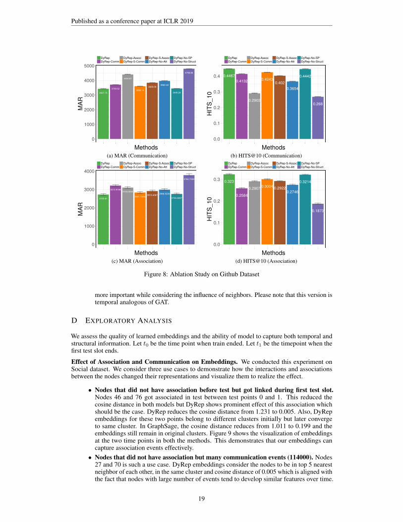
DyRep framework unifies several components that contribute to its effectiveness in learning rich noderepresentation over complex and nonlinear processes in dynamic graphs. In this section, we provideinsights on each component and how it is indispensable to the learning mechanism by performingan ablation study on various design choices of our model. Specifically, DyRep can be divided intothree main parts: Multi-time scale point process model, Representation Update Formulationand Conditional Intensity Based Attention Mechanism. We focus on design choices available ineach component and evaluate them on large github dataset. DyRep in the Figure 8 is the full model.
Multiple Time- Scale Processes. For this component, we perform two major tests:
• DyRep-Comm. In this variant, we make Eq 1., time-scale independent (i.e. remove k)and we train on only Communication Events. But we evaluate on both communicationand association events. Please note that this is possible as our framework can computerepresentations for unseen nodes. Hence during training they will only learn representationparameters based on communication events. It is observed that compared to the full model,the performance of model degrades in prediction for both types of events. But the decline ismore prominent for the Association events compared to Communication Events.• DyRep-Assoc. In this variant, similar to above, we make Eq 1., time-scale independent
and we train on only Association Events. But we evaluate on both communication andassociation events. It is observed that compared to the full model, the performance of modeldegrades in prediction for both types of events. But the decline is more prominent for theCommunication events compared to Association Events.
The above two experiments show that considering events at a single time scale and not distinguishingbetween the processes hurt the performance. Although the performance is hurt more when com-munication events are not considered which may be due to the more availability of communicationevents due to its rapid frequency. We also performed a small test by training on all events but using asingle scale parameter (ψ). The performance for both the dynamics degrades which demonstrates theeffectiveness of ψk.
Representation Update Formulation. For this component, we focus on Eq. 4 and switch off thecomponents to observe its effect.
• DyRep-No-SP. In this variant, we switch off the self-propagation component and we observethat the overall performance is not hurt significantly by not using self-propagation. In general,this term provides a very weak feature and mainly captures the recurrent evolution of one’sown latent features independent of others. It is observed that the deviation has increased forAssociation events which may point to the reason that there are few nodes who have linksbut highly varying frequency of communication and hence most of their features are eitherself-propagated or completely associated with others.• DyRep-No-Struct. In this variant, we remove the structural part of the model and as
one would expect, the performance drops drastically in both the scenarios. This providesevidence to the necessity of building sophisticated structural encoders for dynamic graphs.
Intensity Attention Mechanism. For this component, we focus on Section 3.2 which builds thenovel intensity based attention mechanism. Specifically, we carry following test:
• DyRep-No-Att. Here we completely remove the attention from the structural componentand we see a significant drop in the performance.• DyRep-S-Comm. In this variant, we focus on Algorithm 1 and we only make update to theS matrix for Communication events but do not do it for Association events. This leads toslightly worse performance which helps to see how the S matrix is helping to mediate thetwo processes and not considering association events leads to loss of information.• DyRep-S-Assoc. In this variant, we focus on Algorithm 1 and we only make update to theS matrix for Association events but do not do it for Communication events. This leads toa significant drop in performance again validating the need for using both processes butits prominent effect also shows that communication events (dynamics on the network) is
18
Published as a conference paper at ICLR 2019
3427.75
3709.52
4404.67
3599.143839.09
3962.48
3445.24
4798.86
0
1000
2000
3000
4000
5000
Methods
MAR
DyRepDyRep-Comm
DyRep-AssocDyRep-S-Comm
DyRep-S-AssocDyRep-No-Att
DyRep-No-SPDyRep-No-Struct
0.44670.4132
0.2903
0.42430.402
0.3654
0.4442
0.268
0.0
0.1
0.2
0.3
0.4
Methods
HIT
S_10
DyRepDyRep-Comm
DyRep-AssocDyRep-S-Comm
DyRep-S-AssocDyRep-No-Att
DyRep-No-SPDyRep-No-Struct
(a) MAR (Communication) (b) HITS@10 (Communication)
2722.81
3212.91583104.0034
2831.7224 2913.4067 2986.9226
2755.4837
3784.7059
0
1000
2000
3000
4000
Methods
MAR
DyRepDyRep-Comm
DyRep-AssocDyRep-S-Comm
DyRep-S-AssocDyRep-No-Att
DyRep-No-SPDyRep-No-Struct
0.323
0.2584
0.2907 0.3004 0.29220.2746
0.3214
0.1873
0.0
0.1
0.2
0.3
Methods
HIT
S_10
DyRepDyRep-Comm
DyRep-AssocDyRep-S-Comm
DyRep-S-AssocDyRep-No-Att
DyRep-No-SPDyRep-No-Struct
(c) MAR (Association) (d) HITS@10 (Association)
Figure 8: Ablation Study on Github Dataset
more important while considering the influence of neighbors. Please note that this version istemporal analogous of GAT.
D EXPLORATORY ANALYSIS
We assess the quality of learned embeddings and the ability of model to capture both temporal andstructural information. Let t0 be the time point when train ended. Let t1 be the timepoint when thefirst test slot ends.
Effect of Association and Communication on Embeddings. We conducted this experiment onSocial dataset. We consider three use cases to demonstrate how the interactions and associationsbetween the nodes changed their representations and visualize them to realize the effect.
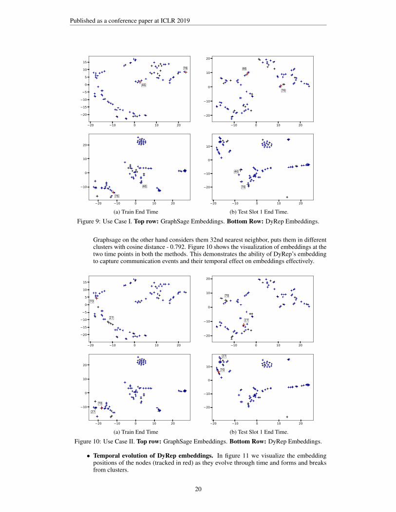
• Nodes that did not have association before test but got linked during first test slot.Nodes 46 and 76 got associated in test between test points 0 and 1. This reduced thecosine distance in both models but DyRep shows prominent effect of this association whichshould be the case. DyRep reduces the cosine distance from 1.231 to 0.005. Also, DyRepembeddings for these two points belong to different clusters initially but later convergeto same cluster. In GraphSage, the cosine distance reduces from 1.011 to 0.199 and theembeddings still remain in original clusters. Figure 9 shows the visualization of embeddingsat the two time points in both the methods. This demonstrates that our embeddings cancapture association events effectively.• Nodes that did not have association but many communication events (114000). Nodes
27 and 70 is such a use case. DyRep embeddings consider the nodes to be in top 5 nearestneighbor of each other, in the same cluster and cosine distance of 0.005 which is aligned withthe fact that nodes with large number of events tend to develop similar features over time.
19
Published as a conference paper at ICLR 2019
20 10 0 10 20
20
15
10
5
0
5
10
15
46
76
10 0 10 20
20
10
0
10
20
46
76
20 10 0 10 20
10
0
10
20
46
76
20 10 0 10 20
20
10
0
10
46
76
(a) Train End Time (b) Test Slot 1 End Time.
Figure 9: Use Case I. Top row: GraphSage Embeddings. Bottom Row: DyRep Embeddings.
Graphsage on the other hand considers them 32nd nearest neighbor, puts them in differentclusters with cosine distance - 0.792. Figure 10 shows the visualization of embeddings at thetwo time points in both the methods. This demonstrates the ability of DyRep’s embeddingto capture communication events and their temporal effect on embeddings effectively.
20 10 0 10 20
20
15
10
5
0
5
10
15
27
70
10 0 10 20
20
10
0
10
20
27
70
20 10 0 10 20
10
0
10
20
27
70
20 10 0 10 20
20
10
0
10
27
70
(a) Train End Time (b) Test Slot 1 End Time.
Figure 10: Use Case II. Top row: GraphSage Embeddings. Bottom Row: DyRep Embeddings.
• Temporal evolution of DyRep embeddings. In figure 11 we visualize the embeddingpositions of the nodes (tracked in red) as they evolve through time and forms and breaksfrom clusters.
20
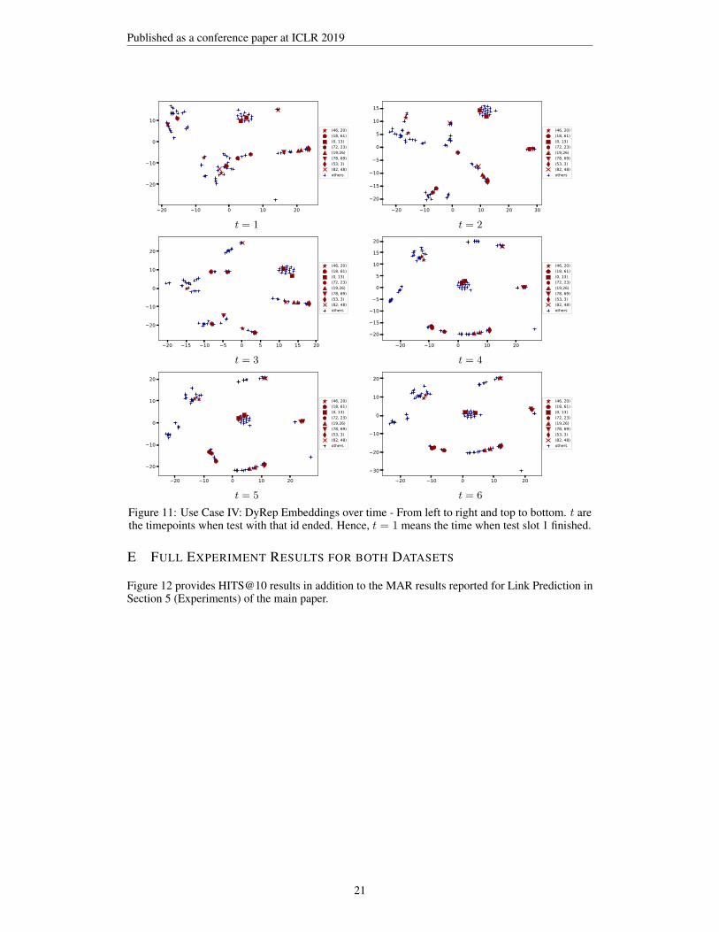
Published as a conference paper at ICLR 2019
20 10 0 10 20
20
10
0
10(46, 20)(18, 61)(0, 13)(72, 23)(19,26)(78, 69)(53, 3)(82, 48)others
20 10 0 10 20 30
20
15
10
5
0
5
10
15
(46, 20)(18, 61)(0, 13)(72, 23)(19,26)(78, 69)(53, 3)(82, 48)others
t = 1 t = 2
20 15 10 5 0 5 10 15 20
20
10
0
10
20
(46, 20)(18, 61)(0, 13)(72, 23)(19,26)(78, 69)(53, 3)(82, 48)others
20 10 0 10 20
20
15
10
5
0
5
10
15
20
(46, 20)(18, 61)(0, 13)(72, 23)(19,26)(78, 69)(53, 3)(82, 48)others
t = 3 t = 4
20 10 0 10 20
20
10
0
10
20
(46, 20)(18, 61)(0, 13)(72, 23)(19,26)(78, 69)(53, 3)(82, 48)others
20 10 0 10 2030
20
10
0
10
20
(46, 20)(18, 61)(0, 13)(72, 23)(19,26)(78, 69)(53, 3)(82, 48)others
t = 5 t = 6
Figure 11: Use Case IV: DyRep Embeddings over time - From left to right and top to bottom. t arethe timepoints when test with that id ended. Hence, t = 1 means the time when test slot 1 finished.
E FULL EXPERIMENT RESULTS FOR BOTH DATASETS
Figure 12 provides HITS@10 results in addition to the MAR results reported for Link Prediction inSection 5 (Experiments) of the main paper.
21
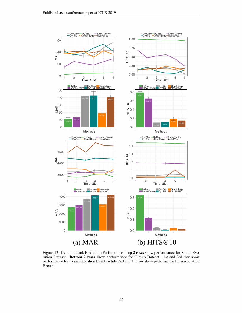
Published as a conference paper at ICLR 2019
0
20
40
60
1 2 3 4 5 6Time_Slot
MAR
DynGemDynTrd
DyRepGraphSage
Know-EvolveNode2Vec
0.00
0.25
0.50
0.75
1.00
1 2 3 4 5 6Time_Slot
HIT
S_10
DynGemDynTrd
DyRepGraphSage
Know-EvolveNode2Vec
11.077313.4774
42.5548 42.74
19.0348
40.5741
0
10
20
30
40
50
Methods
MAR
DyRepKnow-Evolve
DynGemDynTrd
GraphSageNode2Vec
0.787
0.6515
0.1032 0.1236
0.19490.1483
0.0
0.2
0.4
0.6
0.8
MethodsH
ITS_
10
DyRepKnow-Evolve
DynGemDynTrd
GraphSageNode2Vec
3500
4000
4500
1 2 3 4 5 6Time_Slot
MAR
DynGemDynTrd
DyRepGraphSage
Know-EvolveNode2Vec
0.0
0.1
0.2
0.3
0.4
1 2 3 4 5 6Time_Slot
HIT
S_10
DynGemDynTrd
DyRepGraphSage
Know-EvolveNode2Vec
2722.813007.0233
3762.024
4149.9546
3124.5371
4202.606
0
1000
2000
3000
4000
Methods
MAR
DyRepKnow-Evolve
DynGemDynTrd
GraphSageNode2Vec
0.323
0.1173
0.02460.0069
0.02320.01310.0
0.1
0.2
0.3
Methods
HIT
S_10
DyRepKnow-Evolve
DynGemDynTrd
GraphSageNode2Vec
(a) MAR (b) HITS@10Figure 12: Dynamic Link Prediction Performance: Top 2 rows show performance for Social Evo-lution Dataset. Bottom 2 rows show performance for Github Dataset. 1st and 3rd row showperformance for Communication Events while 2nd and 4th row show performance for AssociationEvents.
22
Published as a conference paper at ICLR 2019
F DETAILED RELATED WORK
Static Embedding Approaches. Representation Learning approaches for static graphs can bebroadly classified into two categories – Node embedding approaches aim to encode structuralinformation pertaining to a node to produce its low-dimensional representation (Cao et al., 2015;Grover & Leskovec, 2016; Perozzi et al., 2014; Tang et al., 2015; Wang et al., 2016a; 2017; Xuet al., 2017). As they learn each individual node’s representation, they are inherently transductive.Recently, (Hamilton et al., 2017a) proposed GraphSage, an inductive method for learningfunctions to compute node representations that can be generalized to unseen nodes. Sub-graphembedding techniques learn to encode higher order graph structures into low dimensional vectorrepresentations (Scarselli et al., 2009; Li et al., 2016; Dai et al., 2016). Further, various approaches touse convolutional neural networks (Kipf & Welling, 2017; 2016; Bruna et al., 2014) over graphs havebeen proposed to capture sophisticated feature information but are generally less scalable. Mostof these approaches only work with static graphs or can model evolving graphs without temporalinformation.
Dynamic Embedding Approaches. Preliminary approaches in dynamic representation learninghave considered discrete time approach. (Zhu et al., 2016) propose a temporal latent space modelfor link prediction using nonnegative matrix factorization. (Goyal et al., 2017) uses a warm startmethod to train across snapshots and employs a heuristic approach to learn stable embeddings overtime but do not model time. (Zhou et al., 2018) focuses on specific structure of triad to model howclose triads are formed from open triads in dynamic networks. (Seo et al., 2016) proposes a deeparchitecture based on combination of CNN to capture spatial characteristics and an RNN to capturetemporal characteristics, to model structured sequences which in graph case will lead to discrete timemodel. (Du et al., 2015) develops extends skip-gram based approaches for network embedding todynamic setting where the graphs a re observed as discrete time snapshot and the goal is to learnembeddings that can preserve the optimality of skip-gram objective. NetWalk (Yu et al., 2018) is adiscrete-time dynamic embedding approach specifically designed for anomaly detection which usesclique based embedding techniques to learn vertex representations. Recently, (Trivedi et al., 2017)proposed Know-Evolve, a deep recurrent architecture to model multi-relational timestamped edgesthat addresses the communication process. Unlike our approach, Know-Evolve models all edges at asingle timescale, works for setting restricted to relational graphs and uses only edge-level structuralinformation with no attention mechanism. DANE (Li et al., 2017) proposes a network embeddingmethod in dynamic environment but their dynamics consists of change in node’s attributes over timeand their current work can be considered orthogonal to our approach. (Zuo et al., 2018) proposes adynamic network formation model to learn node representations by employing a Hawkes processto model the temporal evolution of neighborhood for nodes. This work only considers associationevents. (Ngyuyen et al., 2018) proposes a continuous time embedding framework that employs atemporal version of traditional random walks in a simple manner to capture temporally evolvingneighborhood information.
Other models for dynamic networks. There exists a rich body of literature on temporal modeling ofdynamic networks (Kim et al., 2017) that focus on link prediction tasks but their goal is orthogonal tous as they build task specific methods and do not focus on representation learning. Further, there areseveral approaches in graph mining and temporal relational learning community (Loglisci & Malerba,2017; Loglisci et al., 2015; Esteban et al., 2016; Jiang et al., 2016) that consider dynamic networks butare orthogonal to our current work. Research on learning dynamic embeddings has also progressed inlinguistic community where the aim is to learn temporally evolving word embeddings (Bamler &Mandt, 2017; Rudolph & Blei, 2018). (Yang et al., 2017; Sarkar et al., 2007) include some otherapproaches that propose model of learning dynamic embeddings in graph data but none of thesemodels consider time at finer level and do not capture both topological evolution and interactions.(Meng et al., 2018) proposes subgraph pattern neural networks that focuses on evolution of subgraphsinstead of single nodes and links. They build a novel neural network architecture for supervisedlearning where the hidden layers represent the subgraph patterns observed in the data and outputlayer is used to perform prediction. (Yuan et al., 2017) induces a dynamic graph from videos basedon the visual correlation of object proposal that spans across the video. They further propose anLSTM based architecture to capture temporal dependencies over this induced graph and performobject detection. (Jerfel et al., 2017) proposes a dynamic probabilistic model in bipartite case ofuser-item recommendation where the goal is to learn the evolution of user and item latent features
23
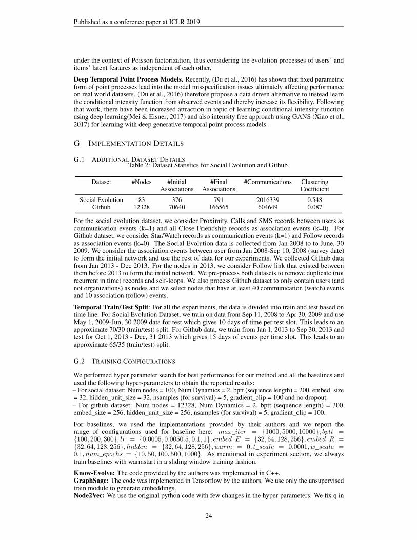
Published as a conference paper at ICLR 2019
under the context of Poisson factorization, thus considering the evolution processes of users’ anditems’ latent features as independent of each other.
Deep Temporal Point Process Models. Recently, (Du et al., 2016) has shown that fixed parametricform of point processes lead into the model misspecification issues ultimately affecting performanceon real world datasets. (Du et al., 2016) therefore propose a data driven alternative to instead learnthe conditional intensity function from observed events and thereby increase its flexibility. Followingthat work, there have been increased attraction in topic of learning conditional intensity functionusing deep learning(Mei & Eisner, 2017) and also intensity free approach using GANS (Xiao et al.,2017) for learning with deep generative temporal point process models.
G IMPLEMENTATION DETAILS
G.1 ADDITIONAL DATASET DETAILSTable 2: Dataset Statistics for Social Evolution and Github.
Dataset #Nodes #Initial #Final #Communications ClusteringAssociations Associations Coefficient
Social Evolution 83 376 791 2016339 0.548Github 12328 70640 166565 604649 0.087
For the social evolution dataset, we consider Proximity, Calls and SMS records between users ascommunication events (k=1) and all Close Friendship records as association events (k=0). ForGithub dataset, we consider Star/Watch records as communication events (k=1) and Follow recordsas association events (k=0). The Social Evolution data is collected from Jan 2008 to to June, 302009. We consider the association events between user from Jan 2008-Sep 10, 2008 (survey date)to form the initial network and use the rest of data for our experiments. We collected Github datafrom Jan 2013 - Dec 2013. For the nodes in 2013, we consider Follow link that existed betweenthem before 2013 to form the initial network. We pre-process both datasets to remove duplicate (notrecurrent in time) records and self-loops. We also process Github dataset to only contain users (andnot organizations) as nodes and we select nodes that have at least 40 communication (watch) eventsand 10 association (follow) events.
Temporal Train/Test Split: For all the experiments, the data is divided into train and test based ontime line. For Social Evolution Dataset, we train on data from Sep 11, 2008 to Apr 30, 2009 and useMay 1, 2009-Jun, 30 2009 data for test which gives 10 days of time per test slot. This leads to anapproximate 70/30 (train/test) split. For Github data, we train from Jan 1, 2013 to Sep 30, 2013 andtest for Oct 1, 2013 - Dec, 31 2013 which gives 15 days of events per time slot. This leads to anapproximate 65/35 (train/test) split.
G.2 TRAINING CONFIGURATIONS
We performed hyper parameter search for best performance for our method and all the baselines andused the following hyper-parameters to obtain the reported results:– For social dataset: Num nodes = 100, Num Dynamics = 2, bptt (sequence length) = 200, embed_size= 32, hidden_unit_size = 32, nsamples (for survival) = 5, gradient_clip = 100 and no dropout.– For github dataset: Num nodes = 12328, Num Dynamics = 2, bptt (sequence length) = 300,embed_size = 256, hidden_unit_size = 256, nsamples (for survival) = 5, gradient_clip = 100.
For baselines, we used the implementations provided by their authors and we report therange of configurations used for baseline here: max_iter = 1000, 5000, 10000, bptt =100, 200, 300, lr = 0.0005, 0.0050.5, 0.1, 1, embed_E = 32, 64, 128, 256, embed_R =32, 64, 128, 256, hidden = 32, 64, 128, 256, warm = 0, t_scale = 0.0001, w_scale =0.1, num_epochs = 10, 50, 100, 500, 1000. As mentioned in experiment section, we alwaystrain baselines with warmstart in a sliding window training fashion.
Know-Evolve: The code provided by the authors was implemented in C++.GraphSage: The code was implemented in Tensorflow by the authors. We use only the unsupervisedtrain module to generate embeddings.Node2Vec: We use the original python code with few changes in the hyper-parameters. We fix q in
24
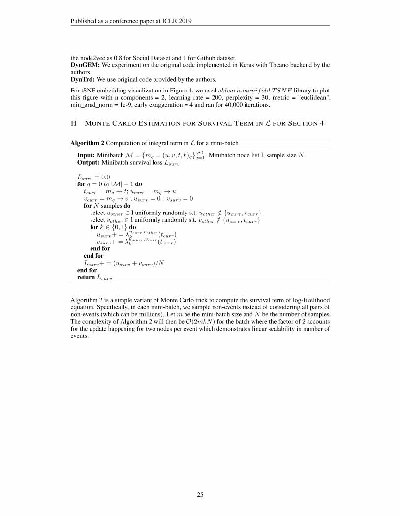
Published as a conference paper at ICLR 2019
the node2vec as 0.8 for Social Dataset and 1 for Github dataset.DynGEM: We experiment on the original code implemented in Keras with Theano backend by theauthors.DynTrd: We use original code provided by the authors.
For tSNE embedding visualization in Figure 4, we used sklearn.manifold.TSNE library to plotthis figure with n components = 2, learning rate = 200, perplexity = 30, metric = "euclidean",min_grad_norm = 1e-9, early exaggeration = 4 and ran for 40,000 iterations.
H MONTE CARLO ESTIMATION FOR SURVIVAL TERM IN L FOR SECTION 4
Algorithm 2 Computation of integral term in L for a mini-batch
Input: MinibatchM = mq = (u, v, t, k)q|M|q=1. Minibatch node list l, sample size N .Output: Minibatch survival loss Lsurv
Lsurv = 0.0for q = 0 to |M| − 1 dotcurr = mq → t; ucurr = mq → uvcurr = mq → v ; usurv = 0 ; vsurv = 0for N samples do
select uother ∈ l uniformly randomly s.t. uother /∈ ucurr, vcurrselect vother ∈ l uniformly randomly s.t. vother /∈ ucurr, vcurrfor k ∈ 0, 1 dousurv+ = λucurr,vother
k (tcurr)vsurv+ = λuother,vcurr
k (tcurr)end for
end forLsurv+ = (usurv + vsurv)/N
end forreturn Lsurv
Algorithm 2 is a simple variant of Monte Carlo trick to compute the survival term of log-likelihoodequation. Specifically, in each mini-batch, we sample non-events instead of considering all pairs ofnon-events (which can be millions). Let m be the mini-batch size and N be the number of samples.The complexity of Algorithm 2 will then be O(2mkN) for the batch where the factor of 2 accountsfor the update happening for two nodes per event which demonstrates linear scalability in number ofevents.
25