DyRT: Dynamic Response Textures

for Real Time Deformation Simulation with Graphics Hardware

Doug L. James and Dinesh K. Pai

Department of Computer Science, University of British Columbia

Abstract

In this paper we describe how to simulate geometrically com-plex, interactive, physically-based, volumetric, dynamic de-formation models with negligible main CPU costs. This isachieved using a Dynamic Response Texture, or DyRT,that can be mapped onto any conventional animation asan optional rendering stage using commodity graphics hard-ware. The DyRT simulation process employs precomputedmodal vibration models excited by rigid body motions. Wepresent several examples, with an emphasis on bone-basedcharacter animation for interactive applications.

1 Introduction

In this paper we present an efficient rendering techniquefor simulating real time dynamic deformations for appli-cations such as character animation. This is achieved us-ing a Dynamic Response Texture, or DyRT, that can bemapped onto any conventional animation (motion captureor keyframe or rigid body dynamics simulation) as an op-tional rendering stage. This is because the complexity ofrendering deformations using DyRT is comparable to light-ing the object. Therefore, every deformable object, large orsmall, can be rendered with realistic dynamic deformationresponses, in real time, on commodity graphics hardware.

The physical realism of DyRT is due to the use of precom-puted modal analyses [22] of dynamic elastic models com-puted using, e.g., the Finite Element Method (FEM) [29].These systems typically have a few clearly dominant dy-namic deformation modes that enable us to produce con-vincing realizations on commodity graphics cards. This isachieved using vertex programs [14] that perform the per-vertex linear superpositions necessary to compute displace-ment and normal vectors.

A second key component of a DyRT is the use of rigidmotion transfer functions for rigid (bone) motion input de-pendence, so that DyRTs respond physically and are notjust “canned vibrations.” This is in contrast to, e.g., severalnVidia vertex program demos [14], such as “warp,” which,although extremely useful in context, have limited physicalfoundations.

In the remainder of this paper we describe the foundationsfor and the process of applying DyRT to objects, with a

particular emphasis on bone-based character animation.

1.1 Related Work

Significant work has been done on simulating dynamic de-formable objects, in areas such as human body modeling andinteractive simulation. Despite the large amount of pioneer-ing work on deformation [25, 28, 15, 1], there continue tobe exciting new applications [18, 17] and improvements insimulation efficiency [2, 6].

Numerous examples of human body modeling exist in theliterature with particular areas of interest being deforma-tions of skin and muscles [27, 9], faces [12], and layeredmodels [5]. Support exists in commercial animation pack-ages, such as Maya, for simulating tissue dynamics. Therehave also been significant recent developments for interactivedynamic tissue simulation, especially for force feedback ap-plications such as surgical simulation [6, 20]. Despite theseadvances, the simulation of transient vibration responses forsecondary animation remains largely absent from the tra-ditional character animation pipeline, and especially so invideo games.

Of particular interest for graphics hardware are data-driven deformation models based on linear superpositionof precomputable global deformation bases [3], which in-clude space warping methods such as FFD. While such mod-els can provide fast simulation and constraint handling forphysically-based dynamic [19, 28] and also static [11, 10]deformable models, we are primarily interested in theiramenability to graphics hardware simulation [14].

For simulating free vibrations of elastic models withmodest amplitudes, global deformation bases based onKarhunen-Loeve expansions from modal analysis providethe optimal description [22, 8]. First introduced to thegraphics community by the pioneering work of Pentland andWilliams [19, 8], more recently they have been used for in-teractive applications involving precomputed or measuredmodal data: stochastic simulation of tree-like structures [23],force feedback [4], and contact sound simulation [26].

Our contribution: This is the first paper to show howto simulate geometrically complex, interactive, physically-based, volumetric, dynamic deformation models in real timewith negligible main CPU costs. We do so with precomputedmodal vibration models stored in graphics hardware mem-ory and driven by a handful of inputs defined by rigid bodymotion.

2 Background on Modal Vibration Models

We briefly summarize the necessary background on modalvibration analysis here, and refer the reader to a suitabletext [22]. The linear elastodynamic equation for a finiteelement model [29],

Mu + Cu + Ku = F, (1)

describes the displacements u=u(t) of N nodes within a vol-ume. The displacement field u is expanded in a modal dis-placement basis

u(t) = Φ q(t) (2)

where Φ denotes the model’s modal matrix, a matrix whoseith column Φ:i represents the ith mode shape, and q = q(t)are the corresponding modal amplitudes, i.e., qi is the modalamplitude of mode shape Φ:i. An important property is thatthe modal matrix Φ is independent of time, and completelycharacterized by values at mesh vertices.

Substituting (2) into (1) and premultiplying by ΦT yields

Mqq + Cqq + Kqq = Q (3)

in which

Mq = ΦTMΦ = diag(mi) (4)

Kq = ΦTKΦ = diag(ki) (5)

Cq = ΦTCΦ (6)

Q = ΦTF (7)

where all of Mq and Kq are diagonal matrices, but for generaldamping Cq is dense. If we make the common assumptionof proportional (Rayleigh) damping

C = αM + βK ⇒ Cq = diag(αmi + βki)

then the system of ODEs are completely decoupled by themodal transformation. This allows the motions due to indi-vidual modes to be computed independently and combinedby linear superposition.

The system of decoupled ordinary differential equationsmay be written as

qi + 2ξiωiqi + ω2i qi =

Qi

mi

, i = 1..n, (8)

where the undamped natural frequency of vibration is

ωi =

√

ki

mi

(in radians) (9)

and the dimensionless modal damping factor is

ξi =ci

2miωi

=1

2

(

α

ωi

+ βωi

)

. (10)

We are interested in underdamped systems for which visibledamped vibration occurs, and this corresponds to ξi ∈ (0, 1).See Figure 1 for example mode shapes and frequencies.

Φ:1 (ω1 =1.00) Φ:2 (ω2≈1.12) Φ:3 (ω3≈1.25) Φ:4 (ω4≈1.44)

Figure 1: Dominant low frequency mode shapes of the bellymodel represent bulk translation and rotation. RGB colorscorrespond to XYZ displacement magnitudes.

Finally, for a system starting from rest at t=0 the solutionfor the ith mode due to forcing Qi(t) is

qi(t) =

∫ t

0

e−ξiωi(t−τ) sinωdi(t− τ)Qi(τ)

miωdi

dτ (11)

where the observed damped natural frequency is

ωdi = ωi

√

1 − ξ2i . (12)

3 Exciting Modes with Rigid Motions

Our goal is to produce realistic modal deformations auto-matically from a conventional bone-based animation specifi-cation, for instance using motion capture data or rigid bodydynamics simulation. Suppose the motion of a rigid body,the “bone,” is specified as a homogenous transformation ma-

trix R(t) =

(

Θ p0 1

)

, where Θ is a rotation matrix. We now

describe how to compute the correct modal forcing functionQi(t) for a deformable object, the “flesh,” attached to a bonesuch as depicted in Figure 2. We describe how to deal withjoints between bones in Sec. 4.2.

Figure 2: Modeling of a thigh finite element model using askeleton and CSG operations.

The velocity of rigid body is represented by its linear ve-locity ν and angular velocity ω. We can therefore view veloc-

ity as a 6×1 twist or spatial velocity1 vector ψ =(

ωT νT)T.

The velocity, rj , of a material point at rj is then given by

rj = [ω]rj + ν = (−[rj ] I )ψ, (13)

where [ω] is the standard skew-symmetric matrix of the crossproduct ω×, and I is a 3-by-3 identity matrix. Using asimple Euler discretization, with constant time step size h,the acceleration of the material point at discrete time stepk is

r(k)j ≈

1

h(r

(k)j − r

(k−1)j ) =

1

h(−[rj ] I ) (ψ(k)

−ψ(k−1)). (14)

Higher order discretizations are similar. Defining

Γ =

−[r1] I−[r2] I

...−[rp] I

we have the acceleration of points on the body as

r(k)

≈1

hΓ(ψ(k)

− ψ(k−1)). (15)

When viewed relative to a coordinate frame attached to thebone, which is accelerating, the D’Alembert force is2

F(k) = Mr

(k)j =

1

hMΓ(ψ(k)

− ψ(k−1)). (16)

This is the forcing function for the vibration in (1). Theprimary modal forcing term Qi/mi in (11) is therefore

M−1q Q

(k) =1

hΦ−1Γ(ψ(k)

− ψ(k−1)), (17)

def= H(ψ(k)

− ψ(k−1)). (18)

1Here we use the traditional kinematic terminology from screwtheory. We refer the reader to any standard mathematical treat-ment on kinematics, such as [16], for more details

2Coriolis forces are negligible here and have been omitted.

We call H=(1/h)Φ−1Γ the rigid motion transfer matrix. Itmaps changes in spatial velocity to modal forces that leadto modal vibrations. It can be precomputed in advance of asimulation and stored. In practice, the forces may be filtered,e.g., scaled and clamped, to avoid extremely large excitationsfrom abrupt motion changes or resonant forcing.

Finally, we need to perform the time-domain convolutionof (11). This can be performed efficiently in discrete timeusing a small IIR digital filter [24, 26]:

q(k)i = 2εi cos θiq

(k−1)i − ε2i q

(k−2)i (19)

+2[εi cos(θi + γi) − ε2i cos(2θi + γi)]

3ωiωdi

Q(k−1)i

mi

where εi =exp(−ξiωih), θi =ωdih and γi =arcsin ξi.

4 Special Considerations

4.1 Normal Calculation

Unlike the displaced vertex positions which can be computedin parallel on a per-vertex basis, vertex normals are compli-cated by the requirement of neighbouring vertex informa-tion. Therefore DyRT objects include an approximate ver-tex normal correction obtained by linearizing the ith vertex’sdeformed normal n′

i about the undeformed value ni,

n′

i = ni +∑

m

Nimqm (20)

where Nim is the ith vertex’s normal correction for mode m.Details are given in Appendix A.

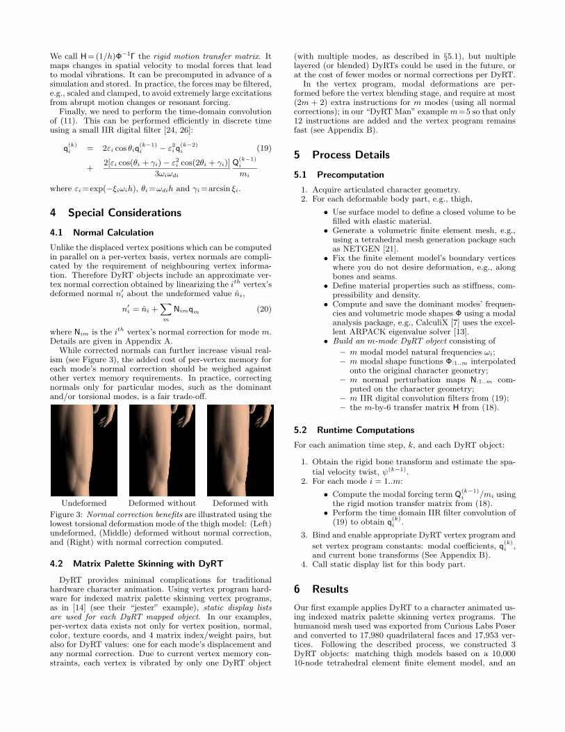
While corrected normals can further increase visual real-ism (see Figure 3), the added cost of per-vertex memory foreach mode’s normal correction should be weighed againstother vertex memory requirements. In practice, correctingnormals only for particular modes, such as the dominantand/or torsional modes, is a fair trade-off.

Undeformed Deformed without Deformed with

Figure 3: Normal correction benefits are illustrated using thelowest torsional deformation mode of the thigh model: (Left)undeformed, (Middle) deformed without normal correction,and (Right) with normal correction computed.

4.2 Matrix Palette Skinning with DyRT

DyRT provides minimal complications for traditionalhardware character animation. Using vertex program hard-ware for indexed matrix palette skinning vertex programs,as in [14] (see their “jester” example), static display listsare used for each DyRT mapped object. In our examples,per-vertex data exists not only for vertex position, normal,color, texture coords, and 4 matrix index/weight pairs, butalso for DyRT values: one for each mode’s displacement andany normal correction. Due to current vertex memory con-straints, each vertex is vibrated by only one DyRT object

(with multiple modes, as described in §5.1), but multiplelayered (or blended) DyRTs could be used in the future, orat the cost of fewer modes or normal corrections per DyRT.

In the vertex program, modal deformations are per-formed before the vertex blending stage, and require at most(2m + 2) extra instructions for m modes (using all normalcorrections); in our “DyRT Man” examplem=5 so that only12 instructions are added and the vertex program remainsfast (see Appendix B).

5 Process Details

5.1 Precomputation

1. Acquire articulated character geometry.2. For each deformable body part, e.g., thigh,

• Use surface model to define a closed volume to befilled with elastic material.

• Generate a volumetric finite element mesh, e.g.,using a tetrahedral mesh generation package suchas NETGEN [21].

• Fix the finite element model’s boundary verticeswhere you do not desire deformation, e.g., alongbones and seams.

• Define material properties such as stiffness, com-pressibility and density.

• Compute and save the dominant modes’ frequen-cies and volumetric mode shapes Φ using a modalanalysis package, e.g., CalculiX [7] uses the excel-lent ARPACK eigenvalue solver [13].

• Build an m-mode DyRT object consisting of

– m modal model natural frequencies ωi;– m modal shape functions Φ:1..m interpolated

onto the original character geometry;– m normal perturbation maps N:1..m com-

puted on the character geometry;– m IIR digital convolution filters from (19);– the m-by-6 transfer matrix H from (18).

5.2 Runtime Computations

For each animation time step, k, and each DyRT object:

1. Obtain the rigid bone transform and estimate the spa-tial velocity twist, ψ(k−1).

2. For each mode i = 1..m:

• Compute the modal forcing term Q(k−1)i /mi using

the rigid motion transfer matrix from (18).• Perform the time domain IIR filter convolution of

(19) to obtain q(k)i .

3. Bind and enable appropriate DyRT vertex program and

set vertex program constants: modal coefficients, q(k)i ,

and current bone transforms (See Appendix B).4. Call static display list for this body part.

6 Results

Our first example applies DyRT to a character animated us-ing indexed matrix palette skinning vertex programs. Thehumanoid mesh used was exported from Curious Labs Poserand converted to 17,980 quadrilateral faces and 17,953 ver-tices. Following the described process, we constructed 3DyRT objects: matching thigh models based on a 10,00010-node tetrahedral element finite element model, and an

abdominal model with 30,000 elements. Precomputationtimes were only a couple of minutes for each DyRT, andmuch larger models could be used. The final character wasanimated with House of Moves motion capture.

In our second example, we apply DyRT to secondary tis-sue in a laparoscopic surgical simulation. In this setting,DyRT helps increase scene realism while allowing the mainCPU to focus on simulating more complex tissue models in-volved in user contact interactions.

Dynamic deformations are inherently difficult to portrayin paper format, however examples in the accompanyingvideo (see Figure 4) illustrate the subtle yet significant im-pact DyRT can have on scene realism. All examples runin real time, at approximately 60 FPS, on a PC with aGeForce3 graphics card; throughout the simulation the run-time cost to the main CPU is negligible.

Figure 4: Examples from video: (Left) A jumping motionthat leads to significant thigh and belly vibrations; (Right)DyRT applied to tissue in a surgical simulation.

7 Summary and Conclusion

We have illustrated the process by which DyRT can be usedto simulate geometrically complex, volumetric, physically-based, dynamic deformation models with negligible mainCPU costs by exploiting commodity graphics hardware.Given our results, we believe that DyRT-based secondaryanimation is an efficient technique to increase the level ofrealism in modern real time applications.

Acknowledgements: We would like to thank the reviewers for

their helpful suggestions, and Edward M. Lichten M.D. for the texture

map image in our laparoscopic surgery example.

A Computation of Normal Correction

We first show how to approximate the face normal for a deformed

triangle. Consider an undeformed triangle with vertices (p0, p1, p2),

a single mode m with amplitude qm

and shape function vertex dis-

placements (u0, u1, u2), so that the deformed triangle has coordinates

(p0 + qm

u0, p1 + qm

u1, p2 + qm

u2). Let U =(p1 − p0), V =(p2 − p0),

δU =(u1 − u0), δV =(u2 − u0), U ′ = U + δU and V ′ = V + δV . For

sufficiently small values of qm

the face normal is

n′

=U ′ × V ′

‖U ′ × V ′‖≈

U × V

‖U × V ‖+ q

m

[

δU × V + U × δV

‖U × V ‖

]

(21)

where the quantity in square brackets is the flat-shaded normal cor-

rection. For smooth shading, normals can be averaged over vertex ad-

jacent faces to obtain the ith per-vertex normal correction Nim from

(20). Alternate approaches using finite differences are also possible.

B Vertex Program for DyRT

# Load vertex pi into R1 and add 5 modal corrections:

MOV R1, v[OPOS]; # R1 = pi

MAD R1, c[DyRT ].xxxw, v[5], R1; # R1 += q1Φi1

MAD R1, c[DyRT ].yyyw, v[6], R1; # R1 += q2Φi2

MAD R1, c[DyRT ].zzzw, v[7], R1; # R1 += q3Φi3

MAD R1, c[DyRT+1].xxxw, v[8], R1; # R1 += q4Φi4

MAD R1, c[DyRT+1].yyyw, v[9], R1; # R1 += q5Φi5

# Load normal ni into R2 and add 5 modal corrections:

MOV R2, v[NRML]; # R2 = ni

MAD R2, c[DyRT ].xxxw, v[10], R2; # R2 += q1Ni1

MAD R2, c[DyRT ].yyyw, v[11], R2; # R2 += q2Ni2

MAD R2, c[DyRT ].zzzw, v[12], R2; # R2 += q3Ni3

MAD R2, c[DyRT+1].xxxw, v[13], R2; # R2 += q4Ni4

MAD R2, c[DyRT+1].yyyw, v[14], R2; # R2 += q5Ni5

# Bone-weighted Vertex Blending: ....

# Transform and Lighting: ....

References[1] D. Baraff and A. Witkin. Dynamic Simulation of Non-penetrating Flexible

Bodies. In Computer Graphics (SIGGRAPH 92 Conference Proceedings), pages 303–308, 1992.

[2] D. Baraff and A. Witkin. Large Steps in Cloth Simulation. In SIGGRAPH98 Conference Proceedings, pages 43–54, 1998.

[3] A. Barr. Global and Local Deformations of Solid Primitives. In ComputerGraphics (SIGGRAPH 84 Conference Proceedings), volume 18, pages 21–30, 1984.

[4] C. Basdogan. Real-time Simulation of Dynamically Deformable Finite El-ement Models Using Modal Analysis and Spectral Lanczos DecompositionMethods. In Medicine Meets Virtual Reality (MMVR’2001), pages 46–52, 2001.

[5] J.E. Chadwick, D.R. Haumann, and R.E. Parent. Layered Constructionof Deformable Animated Characters. In Computer Graphics (SIGGRAPH 89Conference Proceedings), volume 23, pages 243–252, 1989.

[6] G. Debunne, M. Desbrun, A. Barr, and M.-P. Cani. Dynamic real-timedeformations using space and time adaptive sampling. In SIGGRAPH 01Conference Proceedings, pages 31–36, 2001.

[7] G. Dhondt and K. Wittig. CalculiX: A Free Software Three-DimensionalStructural Finite Element Program.

[8] M. Friedmann and A. Pentland. Distributed physical simulation. In ThirdEurographics Workshop on Animation and Simulation, pages 1–17, 1992.

[9] J. Gourret, N. Magnenat-Thalmann, and D. Thalmann. Simulation of Ob-ject and Human Skin Deformations in a Grasping Task. In Computer Graphics(SIGGRAPH 89 Conference Proceedings), volume 23, pages 21–29, 1989.

[10] D.L. James. Multiresolution Green’s Function Methods for Interactive Simulationof Large-scale Elastostatic Objects and Other Physical Systems in Equilibrium. PhDthesis, Institute of Applied Mathematics, University of British Columbia,Vancouver, British Columbia, Canada, 2001.

[11] D.L. James and D.K. Pai. ArtDefo: Accurate Real Time Deformable Objects.In SIGGRAPH 99 Conference Proceedings, pages 65–72, 1999.

[12] Y. Lee, D. Terzopoulos, and K. Walters. Realistic Modeling for Facial Ani-mation. In SIGGRAPH 95 Conference Proceedings, pages 55–62, 1995.

[13] R. Lehoucq, D. Sorensen, and C. Yang. ARPACK Users’ Guide: Solution oflarge scale eigenvalue problems with implicitly restarted Arnoldi methods.Technical report, Comp. and Applied Mathematics, Rice Univ., 1997.

[14] E. Lindholm, M.J.Kilgard, and H. Moreton. A User-Programmable VertexEngine. In SIGGRAPH 2001 Conference Proceedings, pages 149–158, 2001.

[15] D. Metaxas and D. Terzopoulos. Dynamic Deformation of Solid Primitiveswith Constraints. In Computer Graphics (SIGGRAPH 92 Conference Proceedings),volume 26, pages 309–312, 1992.

[16] R.M. Murray, Z. Li, and S.S. Sastry. A Mathematical Introduction to RoboticManipulation. CRC Press, Inc., 1994.

[17] J. O’Brien, P. Cook, and G. Essl. Synthesizing Sounds from PhysicallyBased Motion. In SIGGRAPH 01 Conference Proceedings, pages 529–536, 2001.

[18] J.F. O’Brien and J.K. Hodgins. Graphical modeling and animation of brittlefracture. In SIGGRAPH 99 Conference Proceedings, pages 111–120, 1999.

[19] A. Pentland and J. Williams. Good Vibrations: Modal Dynamics for Graph-ics and Animation. In Computer Graphics (SIGGRAPH 89 Conference Proceedings),volume 23, pages 215–222, 1989.

[20] G. Picinbono, H. Delingette, and N. Ayache. Non-linear and anisotropicelastic soft tissue models for medical simulation. In ICRA2001: IEEE Interna-tional Conference on Robotics and Automation, Seoul Korea, May 2001.

[21] J. Schoberl. NETGEN - An advancing front 2D/3D-mesh generator basedon abstract rules. Comput.Visual.Sci, 1:41–52, 1997.

[22] A.A. Shabana. Theory of Vibration, Volume II: Discrete and Continuous Systems.Springer–Verlag, New York, NY, first edition, 1990.

[23] J. Stam. Stochastic Dynamics: Simulating the Effects of Turbulence onFlexible Structures. Computer Graphics Forum, 16(3), 1997.

[24] K. Steiglitz. A Digital Signal Processing Primer with Applications to Digital Audioand Computer Music. Addison-Wesley, New York, 1996.

[25] D. Terzopoulos and K. Fleischer. Deformable models. The Visual Computer,4:306–331, 1988.

[26] K. van den Doel, P.G. Kry, and D.K. Pai. FoleyAutomatic: Physically-basedSound Effects for Interactive Simulations and Animations. In SIGGRAPH 01Conference Proceedings, 2001.

[27] J. Wilhelms and A.V. Gelder. Anatomically Based Modeling. In SIGGRAPH97 Conference Proceedings, pages 173–180, 1997.

[28] A. Witkin and W. Welch. Fast Animation and Control of Nonrigid Struc-tures. In Computer Graphics (SIGGRAPH 90 Conference Proceedings), pages 243–252, 1990.

[29] O. C. Zienkiewicz. The Finite Element Method. McGraw-Hill Book Company(UK) Limited, Maidenhead, Berkshire, England, 1977.