dzwonczyk -- quantitative failure models of feed-forward neural networks
TRANSCRIPT

QUANTITATIVE FAILURE MODELS OF FEED-FORWARD NEURAL NETWORKS
by
Mark Jonathan Dzwonczyk
B. S. Electrical Engineering, summa cum laude
Tufts University (1984)
Submitted to the Department of Aeronautics and Astronautics
in partial fulfillment of the requirements for the degree of
MASTER OF SCIENCE
in Aeronautics and Astronautics
at the Massachusetts Institute of Technology
February, 1991
© Mark Jonathan Dzwonczyk, 1991The author hereby grants MIT permission to reproduce
and to distribute copies of this thesis document in whole or in part.
Signature of Author4' Department of
Certified by
Aeronautics and AstronauticsJanuary 15, 1991
Wallace E. Vander VeldeProfessor, Department of Aeronautics and Astronautics
Thesis SupervisorI
Certified by
MASSACHUETTS ,Sm rTl ueOF TECHNOLOGY
FEB 19 1991
V Professor Harold Y. WachmanChairman, Department Graduate Committee
LOBAKIES
Aero

QUANTITATIVE FAILURE MODELS OF FEED-FORWARD NEURAL NETWORKS
by
Mark Jonathan Dzwonczyk
Submitted to
the Department of Aeronautics and Astronautics on January 15, 1991
in partial fulfillment of the requirements for the degree of
Master of Science in Aeronautics and Astronautics
ABSTRACT
The behavior of feed-forward neural networks under faulty conditions is examined
using quantitative models. The madaline multi-layer network for pattern classification is used
as a representative paradigm. An operating model of the madaline network with internal weight
failures is derived. The model is based upon the operation of a single n-input processing node
in n-dimensional space. It quantitatively determines the probability of a node failure (incorrect
classification) under specified fault conditions. Resulting errors are then propagated through
network to determine the probability of madaline failure. The analysis is intentionally general
so that the models can be extended to other neural paradigms.
Thesis Supervisor: Dr. Wallace E. Vander Velde, Professor of Aeronautics and Astronautics

ACKNOWLEDGEMENTS
Several people contributed to the successful completion of this thesis. Foremost, my
thesis advisor, Professor Wallace Vander Velde, provided insightful guidance to focus the
work and develop meaningful results. Professor Richard Dudley of the Department at
Mathematics of MIT suggested methods for deriving the probability density functions in
Chapter Three and patiently assisted with questions until the derivations were complete. I
gratefully acknowledge their contributions.
This work was supported by the generous Staff Associate Program of the Charles Stark
Draper Laboratory, Inc. I am thankful to the Laboratory for the privilege to pursue this
research on a full-time basis. I am particularly appreciative to Dr. Jaynarayan Lala, Leader of
the Fault-Tolerant Systems Division, for his patience during my extended leave.
Finally, I am deeply thankful for having a supportive family - including the two new
additions, Natalie and Lianne - which has been indulgent of my unorthodox schedule for the
past 18 months.
Special appreciation goes to Michelle Schaffer for her continued support of my goals.

TABLE OF CONTENTS
A B STRA CT ............................................................................................................................. ii
ACKNOW LEDGEM ENTS ............................................................................................................. iii
1. INTRODUCTION .................................................................................. 6
2. THE ADALINE AND MADALINE MODELS..................................................... 9
2.1. A Single Processing Element: The Adaline............................................ 102.1.1 A daline Classification .................................................................................... 112.1.2 Simplifying the Adaline Equations ................................................................... 12
2.2 Training an Adaline using LMS Techniques .......................................... 132.2.1 Training Based Upon Output Error.................................................................... 152.2.2 Gradient Descent for Least Mean-Squared Error.................................................... 16
2.3 Linear Separability........................................................................ 20
2.4 Many Adalines: Implementing Any Classification Function......................... 23
2.5 Madaline Learning........................................................................ 25
3. FAILURE MODELS ............................................................................... 28
3.1 M odel Criteria............................................................................. 28
3.2 Adaline Operation in n-dimensional Space ............................................ 33
3.3 Single Adaline Failure Model .......................................................... 403.3.1 Single W eight Fault ..................................................................................... 433.3.2 M ultiple W eight Faults.................................................................................. 483.3.3 Summ ary of M odel Equations.......................................................................... 52
3.4 Weight Distributions ..................................................................... 533.4.1 Joint Probability Density Function of Several Weights ........................................ 563.4.2 Probability Density Function of a Single Weight................................................ 66
3.5 Probability of Adaline Failure........................................................... 683.5.1 Closed-Form Solutions .................................................................................. 713.5.3 A M onte Carlo Sim ulation ............................................................................. 723.5.3 Sim ulation R esults....................................................................................... 77
3.6 Probability of Madaline Failure ......................................................... 823.6.1 A n E xam ple................................................................................................. 853.6.2 Som e A nalysis ............................................................................................. 863.6.3 M ultiple Faults in a Network .......................................................................... 89
4. CONCLUSIONS................................................................................... 91
6.1 Sum m ary ................................................................................. 91
6.2 Future W ork.............................................................................. 93

5. BIBLIOGRAPHY .................................................................................. 95
APPENDIX A: MONTE CARLO SIMULATION CODE AND RESULTS............................ 98
A.1 COMGEN.C.............................................................................. 99
A.2 SINGLEPF.C............................................................................. 102
A.3 MULTIPLEPF.C......................................................................... 105
A.4 SINGLEPF.OUT......................................................................... 110
A.5 MULTIPLEPF.OUT..................................................................... 111
APPENDIX B: MATHEMATICAL DERIVATIONS................................................... 114
B.1 Reduction of Gamma Function Ratios ................................................. 114
B.2 Variance of Single Component Probability Density Function....................... 116
B.3 Closed-Form Solution for the Adaline Failure Probability for the SingleZeroed-Weight Fault ..................................................................... 118

CHAPTER ONE
INTRODUCTION
Processing architectures inspired by biological neural systems, so-called neural
networks, have been proven to excel at certain classes of computational problems. These
systems can modify their outputs in order to minimize some error function, essentially
performing non-linear optimization of a multi-dimensional function mapping. This ability to
learn, by self-tuning the processing topology to minimize output error, makes the systems
attractive for implementing functions that are not well understood or difficult to formulate
mathematically. Furthermore, the systems exploit massive parallelism through distributed
storage of global information to achieve a robust realization of this mapping.
Simulations of these architectures have demonstrated their utility for a variety of state
identification problems, particularly in pattern recognition. Hardware prototypes which
implement the algorithms in silicon are now being introduced for such problems. With the
continued advancement of the technology, it is inevitable that operational hardware
implementations will be deployed into meaningful systems in the next five years.
It has been conjectured that the fundamental properties of these systems make them
inherently fault-tolerant. Since state information is dispersed throughout the connection
weights of a large network, the argument goes, loss of any particular local data will not notably
disturb the global state representation, so the systems can withstand a degree of locally
distributed failures. Moreover, their internal thresholding logic is able to restrain the
propagation of errors. The most celebrated property is the architecture's ability to learn. This
means the systems can adapt to internal failures, effectively reconfiguring themselves around
failed elements.
Although these claims may have merit, there has been no examination of neural
network architectures resulting in quantitative metrics of performance under faulty conditions.

To date, the research has provided only qualitative analyses of particular properties and failure
characteristics of select network instantiations; for examples see [11, 33, 35, 36]. Given the
expansive progression of the systems and their likely deployment into substantive applications
in the next several years, it is clear that a quantitative measure of their fault-tolerance is in
order.
This thesis addresses the quantification of the performance of neural networks in the
presence of faults. It is the start of the formulation of a set of criteria that can be applied to
designing ultra-reliable systems.
The approach is to develop a model of the operation of a neural network under faulty
conditions. A particular feed-forward network is chosen as a representative paradigm. A
spatial analysis of the operation of a processing node, or neuron, is used to determine the
effects of faults in the network. Network reliability is determined by a systematic propagation
of the errors from failed nodes.
The purpose of this thesis is not a final pronouncement on the fault-tolerance of neural
networks. The models developed here, and the methods used to construct the models, serve as
an essential foundation for the rigorous analysis that must be partaken to determine the viability
of neural networks as reliable processing architectures.
A general discussion of the computational model of a neural network is omitted from
this work. The reader unfamiliar with the architecture and operation of these connectionist
systems is referred to the many references now available on the subject, including newly
available textbooks [20, 54], summary compilations [3, 46], and the seminal articles that span
the forty years of research of these systems referenced therein.
Chapter Two provides a detailed description of the madaline neural network, the
paradigm selected for study here. Since the failure models constructed later in the text are
based upon the operation of madaline processing elements, called adalines, particular attention
is given to the description of the adaline in that Chapter. This includes adaline learning,
although learning is not addressed in the failure models. It is hoped that this additional detail
will provide the unfamiliar reader with a more substantive understanding of this particular
neuron element.
Chapter Three comprises virtually all the novel work. The formal criteria for the
madaline failure model are presented first. Next, a spatial analysis is used to determine the
operation of an n-input adaline node. In §3.3, failure models of the adaline are constructed.
These models require evaluating the expected values of functions of random variables, where
the variables are the components of an adaline synaptic weight vector. The probability density
functions of those components are next derived. In §3.5, the models are evaluated. Closed-
form solutions for the probability of adaline failure are obtained. Monte Carlo simulations are
used to evaluate those equations. In the final section of Chapter Three, the adaline failure
models are combined to determine madaline failure.
Concluding remarks, including the identification of future research areas, are presented
in Chapter Four.

CHAPTER TWO
THE ADALINE AND MADALINE MODELS
One early computational model which continues to pervade fine grain parallel
architectures is the adaptive linear element, or adaline. The adaline was introduced by Widrow
[60] over three decades ago during the first wave of connectionist activity and was shown to be
a statistically-optimum, trainable classifier. Its utility as a statistical predictor led to its useful
application in real-time adaptive signal processing problems. Currently it is overwhelmingly
used in these contexts [64] and has had commercial success in the telecommunications
industry, particularly as an adaptive equalizer for digital modems and as an echo canceller in
long distance telephone transmissions. With the recent resurgence in neural networks, the
adaline has again become in vogue as a classifier.
In addition to being one of the earliest models for neural processing, the adaline is also
one of the simplest. This makes it ideal for study. Furthermore, it is so general in form, that
other, more complex neural models can be considered specializations of it. For example,
Rosenblatt's perceptron [38] can be considered to be an adaline with additional random fixed
weights and asymmetric Boolean input and output values. Also, if a sigmoid function replaces
the hard-limiter in an adaline, the popular back-propagation learning method [40] can be used
to train a network of adalines. In fact, nearly all non-stochastic connectionist processing
systems are generalized by the adaline model. For this reason, the adaline is chosen as a model
for study here. The failure models which are developed in Chapter Three will similarly be
broad representations which can be tailored to the parameters of other neural processing
models.
This chapter describes the operation of the adaline in both recall and learning phases.
After a review of single element operation and capabilities, the incorporation of the element into
a network of many adalines (a madaline) is discussed. The acronyms adaline and madaline,
incidentally, were coined by Widrow.

2.1. A SINGLE PROCESSING ELEMENT: THE ADALINE
The adaptive linear element is a processing node which performs a weighted sum of its
inputs followed by a hard limiting threshold function. A diagram of an adaline is shown in
Figure 2-1. The adaline has n inputs, xi, i = 1, ... , n, and one output, y. The inputs and
output take on binary values. Unlike conventional Boolean representations, however, the
inputs and output are symmetrically-valued: each may be either +1 or -1. This approach
simplifies the mathematical analysis and allows for inhibiting signals (at level -1) to be readily
utilized.
X 1 w1X2 WS
X n wn
Figure 2-1: An Adaptive Linear Element
Each input is multiplied by a weight value. Thus, there are n weights, wi, i = 1, ..., n,
corresponding to the respective inputs. Weights have continuous values and can be positive or
negative (or zero).
n
A sum of the weighted inputs is first performed in the node. The result is s = Xxiwi.i=1
If the inputs xi and wi are considered to be the elements of two n-dimensional vectors x and w,
X = X2 W W2
-xn. -wn-then the sum can be written as the dot product of the two vectors. Thus,
s = x ow = XTw = WTX
The sum is fed to a threshold element with parameter 0 to yield the node output y. The
threshold function is depicted in Figure 2-2. Thus, the output can be written as a function of
the input and weight vectors and the threshold value:

y= SGN{xow-06} (2-1)
where SGN{ } simply takes the sign of its argument.
X*W
Figure 2-2: Hard Limiting Threshold Function
2.1.1 Adaline Classification
The adaline can classify input sets into two categories, a +1 or -1 category, as specified
by the output. If the argument of eq. (2-1) is set to 0, the decision boundary in n-dimensional
space, 91n , of the adaline is found:
x o w = 0 (2-2)
This is an (n-1)-dimensional plane (a hyperplane) in input space 91n, given by the equation:
n - x 1 w1 - X2 W2 - ... - XnlWn- 1 +0 (2-3)W
n
Classification can be seen with a simple 2-input adaline example (Figure 2-3). The
adaline schematic is shown in part (a) of the figure and the 4 possible input combinations,
(±I1, ±1), are shown in 2-dimensional space in part (b). Suppose input (+1, +1) is assigned to
the set A and the remaining inputs to the complement set, A. Any number of lines in the input
space can be drawn to separate those inputs, that is, to make that decision boundary. A
particular one is shown in the figure. The line has the equation x2 = -X1 + 1.
From eq. (2-2) the decision boundary of this example is x1wl + x2w2 = 6, which can
be manipulated, as presented in eq. (2-3), to obtain a linear equation for x2 in terms of xl and
0:

W1x2 = - X1 + (2-4)W2 W2
wi 0The resulting line (a hyperplane of dimension 1) has a slope of - - and an x2-intercept of w
If w1, w2, and 0 are all set to 1, eq. (2-4) is x2 = -X1 + 1, precisely the line drawn in Figure 2-
3b. Now if the set A is equated with a y value of +1 and the set A with a y value of -1, the
adaline with w, = w2 = 0 = 1 will perform the desired classification, creating the decision
boundary shown in Figure 2-3b. By varying the parameters Wl, w2 and 0, other decision
boundaries can be drawn.
(-1,.
xi WX2 W2Y
(-1,
Xi
1)
(a) Schematic Representation (b) Input Space
Figure 2-3: The 2-input Adaline
2.1.2 Simplifying the Adaline Equations
One of the characteristics of the adaline, and of all neural network processors, is
regularity. Regularity affords easy replication and streamlines mathematical analysis.
Although it may be obvious that the input weights of an adaline can be readily modified to
perform a classification function, the requirement to change the threshold parameter, 0, for
each adaline does not appear to be a simple task. In the model described by eq. (2-4), a new
threshold function must be constructed (with a new 0) in order to move the x2 intercept of the
decision boundary.
In fact, the model can be altered to make the adaline structure more regular. The
threshold function is simplified by setting 0 = 0 for all adalines. The variability of the

threshold parameter can be recovered by adding a new input, x0 a +1, and weighting that input
by wo. Thus, the strict definition of the adaline function, originally described by Widrow [60]
is given by
y = SGN {xiwi (2-5)
The adaline is shown in Figure 2-4.
+1
X1X2
Xn
y
Figure 2-4: The Adaline
The general n-1 dimensional hyperplane is determined by
xn -wo - xlwl - x2W2 - ... Xn-1Wn-1 (2-6)Wn
The new weight, wo, is -0 of the original model. In the 2-input example, eq. (2-4) becomes,
wl w0x2 = X1 -wo
w2 W2
Figure 2-4 and eq. (2-5), where x0 =- +1, will be used for the remainder of this work as the
adaline definitions.
2.2 TRAINING AN ADALINE USING LMS TECHNIQUES
The adaline has the ability to classify its inputs into one of two categories. In the
example of the previous section, a two input adaline was programmed to perform as a logical
AND gate. That is, if -1 is equated with logical FALSE (F) and +1 is equated with logical TRUE
(T) , then the output, y, is T if and only if input xi is T AND input x2 is T; otherwise y is F.
With w1 = w2 = +1 and wo = -1 (the weight values have no logical significance and are
coincidentally +1 and -1), the AND function, tabulated below, has been constructed.

-1, F
-1, F
+1, T
+1, T
-1, F
+1,T
-1, F
+1, T
y = (x 1 AND x2 )
-1, F
-1, F
-1, F
+1, T
Figure 2-5: Logical AND Function Constructed by the 2-input Adaline of §2.1
In this example, the adaline was programmed. That is, eq. (2-6) was analytically
solved for wo, wl, and w2. (There were three unknowns and 1 equation, so two variables
were arbitrarily set to +1.) Programming the weights of an adaline becomes difficult,
however, as the number of inputs grows large. If the analytic classification function is not
known (if the location of the hyperplane is not known) programming becomes impossible. 1
For example, suppose the input vector represents a 2-dimensional pattern of a binary image and
it is desired to have an adaline determine if that image is a filled-in circle. It would be a very
difficult task to identify a priori the placement of the hyperplane decision boundary on the input
space.
As its name implies, however, the adaline can be made to adapt itself in order to
perform the classification. When presented with the set of inputs and corresponding outputs,
the adaline can adapt its weights so that the appropriate classification will be performed. This
process is called learning and is one of the fundamental properties of neurocomputing systems.
It obviates the need for analytical solutions to classification problems and the ensuing
programming which is requisite for all conventional computing systems. The neural approach
also allows, simply upon presentation of examples, abstraction of concepts to statistically
resolve the key features of the input space and generalization to situations never before
encountered.
1. If the hyperplane location is known, a look-up table or other less complex method could be used to performthe classification.

In this section, adaline learning is examined. It is shown that the adaline can learn a
classification in an optimum manner by using only information available only locally, that is,
by using only the input and weight vectors, the desired output, and the current output, which
may be in error. The adaline adjusts its weights to minimize this error.
2.2.1 Training Based Upon Output Error
The adaline can learn a classification function simply upon repeated presentation of
pairs of input vectors and corresponding desired outputs. This process is called supervised
learning because a supervisor is required to present the adaline with the desired output category
for the input vector. 2 Thus, the availability of an output training signal is assumed. For large
input vectors (representing, for example, a two dimensional pattern) this is a non-trivial
assumption: it is not always clear which is the appropriate classification, and if it were a look-
up table may well suffice for the task.
Consider the following process. A specific input vector x 1 with a desired
classification, Yd, is presented to an arbitrarily configured adaline. The adaline settles to an
output, y, based upon its arbitrary weights, w. An error signal, e, is constructed from Yd and
y. The signal E is a penalty or cost function of output y with respect to Yd , = C(y, Yd). The
weights are then systematically adjusted until the error is zero or the cost is minimized in some
reasonable sense. If the error is zero, then the adaline has been properly adapted and it has
"learned" the classification of that specific input vector xl. This process can be repeated for
multiple pairs of vectors and desired classes, { Xi, Ydi }. If the cost is optimally minimized, the
adaline has learned to the best of its ability. When the error is zero for all vectors, the adaline
has learned the appropriate classification.
2. Another form of learning, called unsupervised or self-organized, obviates the need for the training input.Two of the more popular unsupervised learning methods are Kohonen's self-organizing map [26] and theadaptive resonance theories of Grossberg and Carpenter [52].

The principal challenge to creating a supervised learning scheme is the derivation of a
systematic weight modification method which will converge to some optimally minimum net
error. For example, in a poor learning scheme, the weight modifications which may be
required to learn the classification of a second vector, X2, may completely destroy the learned
classification of xl.
Consider the cost function as a surface above a multi-dimensional plane of its
arguments. If the cost function is quadratic in its arguments, its surface will be a paraboloid
with a single (global) minimum. The principal method of iteratively finding the minimum of
such a surface from an arbitrary starting location is gradient descent [63]. In this method, a
change in the arguments of the cost function is made in the opposite direction of the gradient of
the surface, that is, in the direction of steepest downhill change. Figure 2-6 illustrates gradient
descent with one argument only.
X = Xk
Figure 2-6: Gradient Descent Minimizing with One Argument
Because the adaline performs a linear sum of weighted inputs, a cost function which is
quadratic with adaline weights can be constructed and a gradient descent method can be used to
iteratively modify the weights until the minimum is reached. Finding that cost function was the
breakthrough of Widrow which has made the adaline widely applicable.
2.2.2 Gradient Descent for Least Mean-Squared Error
Consider the error with respect to the linear sum. Let the error signal be equal to the

difference between the desired output, Yd, and the sum, s, and be denoted es. The presence of
a possible negative value for es is bothersome since minimizing this error would lead to driving
the adaline to a negative error, not a minimum net error. To avoid this problem, it is
appropriate to square the cost function. Thus the error signal can be defined as
(s) 2 = (Yd- S)2
= (Yd - xTw)2
Clearly, (es) 2 is a quadratic function of the weights w. It is a paraboloid with a global
minimum w* (at a constant x and yd), as illustrated in Figure 2-7.
Figure 2-7: Minimum of a Parabolic Cost Surface
The actual output error is ey (Yd - y). But, (Fy) 2 is a monotonic function of (Es) 2 [60].
That is, as (Es) 2 increases, (ey) 2 increases; as (Es)2 decreases, (Ey) 2 decreases. Minimizing
(Es) 2 will therefore minimize (ey) 2. This means that w*, the minimum of the parabolic function
(Es) 2, provides the least mean-squared output error of adaline.
In both the training and recalling phase of adaline operation, the input vector is assumed
to be random. Thus (Es) 2 will be a random variable with an expected value E { (Fs)2 }. From
the definition:
E { (es)2 } =E { (ydd - xTw) 2
and since xTw = WTX (a scalar),
. . i

= E { (yd - wTx) (yd -xTw)}
= E { (yd)2 - 2ydXTW + WTXXTW I
E{(Es)2 } = E{(yd)2 } -2E{ydxT}w +WT E(xxT}w
The input vector is assumed stationary, that is, its statistics do not vary with time. If p is
defined as the cross-correlation of the input vector and the desired response scalar and R is the
input correlation matrix:
p - E{ydX)
R - E{xxT}
then
E { (cs)2 } = E { (yd) 2 }- 2 pTw + wTRw
Recognize that Yd = +1, so that E (yd)2 } = 1:
E { (s) 2 } = 1 - 2 pTw + wTRw (2-7)
It is desired to minimize this expected value. Gradient descent in weight space is used.
The gradient of E { (e~) 2 } is
V E (s) 2} - E{ (s)2 } (2-8)
and from eq. (2-7)
VE{ (e~s)2 } =- 2p + 2Rw (2-9)
The argument of the minimum value, w*, is reached when the gradient is zero:
0 = V Et (es) 2 } =-2p + 2Rw
which yields
w* = R- 1p
The minimum error is found by inserting w = w* into eq. (2-7):
E { (Es) 2 } = 1 - 2 pTR-lp + pTR-1RR-lp
= 1 - 2 pTR-1p + pTR-1p

E(Es)2 } = - pTR-lp
The gradient descent method dictates the change from an arbitrary weight vector, Wk, to
the next Wk+1, where the index represents an iteration number:
AWk =-}Vk
Wk+1 = Wk + AWk
where .t is a constant which determines the rate of change and guarantees convergence. Using
eq. (2-9)
Wk+1 = Wk + t(2p - 2Rw) (2-11)
Unfortunately, all statistics required to implement eq. (2-11) are not known. If they
were, w* = R-1 p could be used to minimize E t (F,)2 } directly. Instead of the true gradient, an
estimate of the gradient must be made.
The easiest estimate of the expected value of (es) 2 is (Es)2 itself. That is, defineAVk - E(ps)2 = V E t (es)2}
= (Yd - XTw) 2
= -2 x(yd - xTw)A
Vk = -2xgs (2-12)
So that the weight change using the estimated gradient is
A
AWk = -lrk
so Wk+1 = Wk + 2txes (2-13)
Note the simplicity of this algorithm: all information required for each weight change is local to
the adaline. The new weight is simply the current weight modified in the direction of the input
vector (x) proportioned by the adaline sum error (Es).
Although an estimate of the gradient is used in the iteration process, convergence to the
minimum error, as dictated by the true gradient descent, is still guaranteed. To see this, take
the expected value of the gradient estimate. From eq. (2-12),
(2-10)
AEtVk} = E{-2x(yd- xTw)}
-2EX { (yd- xTw)}
= -2E { xyd -xxTw}A
E{Vk} = -2E{xydI +2E{xxTw}
which from the definitions becomes
A
E{Vk} = -2p+2Rw
which is the definition of the gradient from eq. (2-9). Thus
A
E{Vk} = Vk
Eq. (2-13), often called the Widrow-Hoff or Delta rule, presents a method for adjusting
the weights of an adaline which minimizes the output error. If the input training vectors are
independent over time, for a large number of trials the Delta rule will converge to the minimum
error given in eq. (2-10) [63].
2.3 LINEAR SEPARABILITY
The perceptive reader will note that a single line cannot create a decision boundary for
all possible binary classifications of adaline input space in Figure 2-3. Only classifications
which are determined with a single line can be implemented. Inputs which can be classified in
this way are called linearly separable. In n-dimensional space, linearly separable inputs can be
separated by an n-1 dimensional hyperplane.
The notorious example of linearly inseparable classification is the Boolean exclusive-or
(XOR) function. In two dimensional adaline input space, the XOR function is TRUE (+1) for the
set of inputs which differ in sign, namely, (-1,+1) and (+1,-1). The function is depicted in
Figure 2-8. As can be seen, no single line can separate the two classes of inputs.
In their compelling 1969 treatise Perceptrons [32], Minsky and Papert argued that the
inability of neuronal elements such as the adaline to perform linearly inseparable classifications

X2= +1--
(-1,+1) 0
(-1, -1) 0 -
-y = -1
- (+1, +1)
a 2 X1
Ho (+1,-i)
(a) Input/Output Function (b) Input Space Classification
Figure 2-8: The 2-input XOR function
severely limited their computational capacity. Their work was so convincing (because it was
mathematically rigorous) that research at the time went into remission for well over a decade.
The XOR problem epitomizes their arguments.
For the 2-input adaline, there are 22 possible input combinations. Since the output is
binary each of the 4 input combinations can take on 1 of 2 values. Thus, there are 2(22)
possible classification functions. Of these 16, only 2 require classification of linearly insep-
arable functions: the XOR and its complement, the XNOR. However, in the more general n-
input adaline, there are 2(2n) possible input classification functions and the number that require
classification of linearly inseparable inputs becomes a larger fraction of the total. It has been
shown that as n approaches infinity, the percentage of linearly separable classification functions
in the ensemble becomes zero [56]. Thus, for a reasonably large adaline, Minsky and Papert's
concerns are legitimate.
The inability of the adaline to perform linearly inseparable classifications is clear from
the semantics: the decision boundary created by an adaline in its input space is linear and can
therefore only separate inputs which are linearly separable. To implement a non-linear
separation, a non-linear decision boundary must be constructed.
Recall that the decision boundary is determined by setting the argument of SGN {* } in
eq. (2-1) to zero. In that equation, the argument is s = 0 + w x1 + ... + wnxn, a linear
Yxl1
-1
1
1
x 2
-1
1
-1
1
-1
1
1
-1

function of the inputs. If this argument is changed to a generalized non-linear function of the
inputs, non-linear separation can be implemented.
For example, let the non-linear sum, s', be defined as
S' = w0 + wlx1 + wll(Xl) 2 + W2X2 + W22(X2) 2 + Wl2X1X2
and the weights to be programmed as wo = 0.25, Wi = w2 = 0, Wi1 = w22 = -0.5, and wl2 = -
0.875. These parameters yield the decision boundary of Figure 2-9, where the inputs inside
the ellipse are classified as y = +1.
X1
Figure 2-9: Non-Linear Decision Boundary for the XOR Function
Clearly, the key to implementing linearly inseparable classifications is to apply a non-
linear function to the inputs. The question then becomes how to create the non-linearity. After
all, the elegance of the LMS algorithm is due to the linear combination of the inputs yielding a
quadratic error surface in weight space.
In fact, a non-linearity is readily available in the form of the adaline threshold. The
inputs can be "preprocessed" with adalines to obtain a non-linear function of the inputs. Since
the threshold is not a generalized polynomial, not all classifications can be implemented with
one layer of preprocessing. As shown in the next section, two preprocessing layers - for a
total of three layers - are required to implement any arbitrary mapping. 3
3. Viewed in another way, adalines which implement the logical NAND can be used as building blocks forlarger functions [2]. Since all logical functions can be constructed from NAND elements, a network of

2.4 MANY ADALINES: IMPLEMENTING ANY CLASSIFICATION FUNCTION
It is clear that a non-linear operator must be applied to the inputs of an adaline in order
for the device to perform a linearly inseparable classification. If adalines are used to realize this
preprocessing, a layered network of many adalines - a madaline - is created.
A madaline is a network of layers of adalines. A three layer madaline with equal
number of adalines per layer is shown in Figure 2-10. (Weights between adalines are not
shown for simplicity.) In general, the number of adalines per layer can vary. Full connectivity
between layers is usually assumed (a weight of 0 is equivalent to an open connection), but the
topology is strictly feed-forward: no feedback paths are allowed.
single n-input adaline
x .
x
x
Yl
Y2
Yn
Figure 2-10: A Three Layer Madaline
In Figure 2-3, a single adaline formed a single line in the adaline input space. Two
adalines with the same inputs can form two lines. In general, m adalines can form m decision
hyperplanes.
Figure 2-3b is repeated below (Figure 2-11b) with a new decision line separating an
additional classification, B and B. Two adalines, configured as shown in Figure 2-11 la, are
used to create these two lines.
adalines can implement any logical function.

+1 A X2
Y4(-1,+1)
yI
Y2
(-1, -1) S -
* (+1, +1)
X1
\* (+1, -i)B,
+1 T '(a) Schematic Representation (b) Input Space
Figure 2-11: Additional Classification of Adaline Input Space
The two outputs, Yi and Y2, which classify all four inputs into both classes A (A) and
B (B), respectively, can be fed to a third adaline. Since A is represented by yi = +1 and B as
Y2 = +1, these two outputs can be used as the inputs for the third adaline. To implement the
XOR, the desired classifying set is A AND B, so the third adaline must implement the Boolean
function y3 = y1 AND Y2, a linearly separable function realized with wo = -1, wl = -1, and w2
= +1. The three adaline structure with the classification of the inputs is shown in Figure 2-12.
Thus the XOR function, which is linearly inseparable, can be implemented with 3 adalines
assembled in a two layer structure.
+1
y3
+1
Figure 2-12: A Three Adaline XOR
The network of Figure 2-12 forms a region { A AND B } in adaline input space by
x
x
+1 •Atf' X2

bounding it with 2 decision lines. Additional regions can be formed using additional adalines
in the second layer. More complex regions can be formed using additional adalines in the first
layer. In principle, a two layer madaline with sufficient number of adalines in each layer can
form any number of convex regions in the input space. If convex decision regions are all that
is required, a two layer network will suffice.
To implement decision regions which are more general than convex, an additional layer
is needed [28]. An adaline can create arbitrary regions from convex regions, so the convex
regions created in the second layer must be fed to a third layer. The second layer becomes
"hidden", forming an internal representation of the input space [40]. The third layer which has
formed decision boundaries of arbitrary geometry can implement any classification function
and acts as an output layer.
Thus, a three layer madaline neural network with sufficient numbers of adalines in each
layer can implement any classification function. A formidable problem, however, is
determining the number of adalines required for a particular classification task. A larger
problem is assigning the weight values. For n adalines in a network, the assignment of
weights to implement a classification function requires satisfying O(n 2) constraints. Similar to
the single input adaline, if the analytic classification function is not known - if all of the
boundaries of the classification region are not known a priori - learning must be used. This is
the subject of the next section.
2.5 MADALINE LEARNING
Learning in a madaline network is similar to adaline learning in that it is based upon
error feedback. Madaline learning, however, is plagued by the problem common to all non-
linear multi-layer adaptive neural networks: credit assignment [32]. The dilemma is
determining the effect of network parameters, namely, the synaptic weights, on the output error
of the network.

In a single adaline, a parabolic cost function can be created and the minimum error can
be found through gradient descent. In a multi-layer network, the cascaded non-linearities
prohibit the construction of a parabolic error surface. The output error surface is arbitrarily-
shaped. A global minimum may exist, but reaching it through gradient descent is virtually
impossible due to the local minima which permeate the surface.
The back-propagation learning rule [40] exploits the sigmoidal nature of its neuron
threshold function. Using the derivative chain rule, the change in output error for network
parameters is propagated backward through the network layers.4 Even so, convergence to an
absolute minimum error is not guaranteed. The step threshold of the adaline has an infinite
derivative and thus prohibits such an approach.
The madaline network has evolved in stages since its original introduction 30 years ago
[56]. The learning rules have also evolved with the architecture. Through the history,
however, all madaline learning rules have been based upon the simple principle of minimal
disturbance. In Widrow's words [64]:
When training the network to respond correctly to the various input patterns, the"golden rule" is to give the responsibility to the neuron or neurons that can mosteasily assume it. In other words, don't rock the boat any more than necessaryto achieve the desired objective.
The minimal disturbance principle is best embodied by madaline learning rule II (MRII)
[67]. Consider a network of adalines which is presented with an input pattern, x. If the output
classification, y, is in error, then weights of the adalines in the first layer are perturbed to
determine their effect on the output. The adaline in the first layer whose weighted sum is
closest to zero is perturbed first. That is, the adaline whose weight change will have the
minimum disturbance on the network is given a first attempt at reducing the error. The
perturbation is such that adaline output changes sign. If this perturbation reduces the network
4. Since back-propagation uses the gradient descent techniques of Widrow, it is sometimes referred to as thegeneralized Delta rule.

output error, the weight changes are accepted; otherwise, the changes are rescinded. The first
layer adaline whose weighted sum is the next closest to zero is then perturbed. This process
continues for all first layer adalines and then to all subsequent layer adalines until the network
error is zero or all adalines have been perturbed. This tedious process is not computable
locally, but has shown acceptable results.
The next generation of madaline learning rules, MRIII [4], propagates an estimate of
the error gradient backward through the network layers. It has been shown to converge to the
weights which would have been found using back-propagation. That is, the madaline rules are
globally calculated versions of the local back-propagation of errors. It is important to
remember, however, that convergence of madaline to zero error using any rule - or for that
matter, convergence of any multi-layer perceptron network to zero error - cannot be
guaranteed, except for particularly well-behaved input sets.

CHAPTER THREE
FAILURE MODELS
In this chapter, a failure model of the adaline is constructed. The approach is to
examine the operation of an n-input adaline in (n+1)-dimensional space and is an extension of
Stevenson's weight sensitivity analysis work [50]. Given specific fault modes, the model can
be evaluated to determine the probability of adaline failure under faulty conditions. The models
of many adalines connected in a feed-forward topology are then combined into a madaline
failure model. Since the madaline architecture is a generalization of many different feed-
forward neural networks, the models can be used for further study of other networks.
Clarifying definitions of the failure model and fault modes which will be considered are
presented first. Next, the operation of a single n-input adaline in 9 n + 1 is described. From
this, a failure model of the adaline is developed which treats all failures as weight perturbations
and describes the operation of an adaline as a function of the perturbation. After identification
of the probability distribution for the adaline weights, the specific fault modes are inserted into
the failure model and the probabilities of failure are determined. Extensions are then made to
the madaline network.
3.1 MODEL CRITERIA
In this work, a failure model of an adaline is desired which can be extended in some
manner to evaluate a madaline network of arbitrary size. Ideally, the adaline can be considered
as a "black box" with inputs, outputs, and an internal mapping function. The goal is to
determine the probability of failure of the black box. Extension to a madaline network failure
model can be realized through a systematic assembly of black box models. The probability of
madaline failure can be determined from a combinatorial aggregation of adaline failure
probabilities.

A necessary foundation for achieving that goal is a clear understanding of the terms
associated with dependable computing. In the vernacular of the technical community [5], the
adaline is a resource which provides a service. This service is a mapping of an input vector, x,
to an output scalar, y, by a specification, S, such that y = S(x). If the actual output, y', does
not agree with the specified output (for the same input), then the output y' is in error and the
resource has failed. The failure is caused by one or more internal resourcefaults.
Figure 3-1 depicts the adaline as a black box resource. It provides the specified service
stated in eq. (2-5):n
y = SGN{• xiwi } (2-5)'i= 0In this context, the adaline service is binary classification for the n-dimensional input vector.
The linear summer and threshold units in the adaline provide the capability for that service.
The particular classification function is the service specification and it is determined by the
weight vector 1, w = [wo w, ... wn]T. Note that the adaline is being considered only in its
feed-forward (or recall) operation: no learning mechanism is associated with the resource of
Figure 3-1.
X 1
X2INPUTS
xn
y OUTPUT-
RESOURCE
Figure 3-1: The Adaline as a Black Box Resource
With these basic definitions in hand, the purpose of the failure model can be stated
1. Normally one would say that the specification determines the weight vector, but this discussion is forgeneral adaline operation. A weight vector can be determined through programming or training, but even anarbitrary weight vector will result in some service specification.

succinctly: the model will determine the (conditional) probability of adaline failure, given some
internal adalinefault. In other words, assuming the adaline weights have been set such that a
specified service is provided and given some internal adaline fault, the failure model will
determine the probability of the misclassification of the input vector. Note the underlying
assumption that a fault-free adaline does not misclassify. By definition, an adaline with a
specified weight vector provides a specified service. It is true that a single adaline is incapable
of providing a linearly inseparable classification service, but a fault-free adaline is guaranteed to
perform the service specified by its weights.
Since the adaline is defined as the resource of interest in this work, it should be clear
that the failure model does not consider adaline training. Although adaptability is an important
fault-tolerance attribute, by no means does it guarantee that the adaline can learn around all
possible faults. Consideration of adaline adaptability requires a thorough evaluation of a
specific learning rule in the context of the assumed topology. Instead of examining the
performance of particular learning schemes, this work is meant to evaluate the fault-tolerance of
a neural network in the recall phase. The work can be compared to similar studies of
heteroassociative or autoassociative memories (a.k.a., content addressable memories) when the
input vector is incomplete. 2 Here, the probability of (correct) madaline recall will be
determined, given some internal memory fault.
Since the failure model assumes some internal resource fault has occurred and
determines the probability of correct operation (classification) conditioned on this event, the
selection of the fault event is the underpinning of a valid failure model. In Chapter Two, the
weight vector was shown to create a hyperplane which separates the adaline input space.
Changes in the weight vector change the adaline classification by moving the hyperplane. A
reasonable fault to consider, then, is a perturbation of the weight vector. In fact, except for
2. Kohonen [25] offers an extensive review of these systems.

pathological cases3 , faults in the summer or threshold units can be modelled as weight faults by
moving the decision hyperplane to emulate their effect and altering the weight vector to produce
the new hyperplane. For example, a stuck-at-one failure occurs when all inputs are classified
as y = +1. A weight vector of w = [a 0 ... 0]T, a > 0, could be used to model this failure.
From a practical perspective, since weights far outnumber 4 other components in a physical
implementation, weight faults are the most meaningful events for study. Furthermore, in a
practical setting weights are likely to be more failure prone since they must be a dynamic
media, while the summer and threshold units can be constructed from fixed electronic devices.
Thus, for this work, the following supposition applies: Since the adaline failures are
considered to be input misclassifications and are caused by some internal adaline fault, and
adaline weights determine the classification function by positioning the decision hyperplane,
then all faults are considered weight faults or can be emulated by weight faults.
The next logical question concerns the type of weight fault: which weight faults should
be considered in the analysis? In search of an answer to that question, consider an electronic
implementation of an adaline. An input would be amplified by a weight value which can be
positive or negative. A physical realization, however, must place a limit on the maximum and
minimum values which can be achieved. For example, an operational amplifier will saturate at
its rail voltages. One reasonable fault mode to consider, then, is the driving of the weight from
its preset value to one of its possible rail values. This will be called a railfault. For simplicity,
assume the rails are at ±1. A rail fault, then, is a change in a weight from its original value to
its rail value, wi -- ±1.
A second likely fault is the disconnection of a synapse such that the input at that
3. A pathological failure would be an adaline which no longer implements a linear hyper-"plane", i.e., thedecision boundary is non-linear.
4. In a single madaline layer with n adalines, there are n2 weights and n summers and threshold units. For n =20, weights account for over 90% of the components; at n = 100, representing a pixelated 10 by 10 windowfor image recognition, weights account for 98% of the components.

synapse does not contribute to the internal summed value. This disconnection can be
represented by a zero weight value for that synapse, wi --+ 0. This fault will be called a zeroed-
weight fault.5
A failed adaline produces an output y' which has the opposite sign of its non-failed
output. Adalines in the adjoining layer whose inputs are attached to the failed adaline thus
receive an erroneous input. With some probability, a non-faulty adaline with an erroneous
input will produce an output different than the output with error-free inputs. That is, with
some probability the adaline with an erroneous input behaves as if it had failed. This failure
can be modelled as a weight fault, the fault being a change of sign in the weight component.
Although its physical manifestation is unlikely, such a fault is paramount for modelling errors
which propagate through the network and will be considered as an adaline fault mode. This
fault will be called a sign-change fault.
Of course, many other classes of weight faults exist and could be enumerated ad
infinitum. The rail fault and the zero weight fault represent the extreme fault modes which
could beset an adaline. Using these faults in the failure model should result in a conservative
estimate of the probability of correct adaline operation since it is unlikely that a small weight
perturbation would cause an adaline to fail while a weight change to -1, +1, or 0 would not.
The sign-change fault is useful in propagating adaline failures through the network. These
three fault modes will be used in the remainder of this work to determine their effect on adaline
operation.
A final pronouncement on faults is in order before the model criteria are summarized.
The model developed in the subsequent sections is a static one, that is, the analysis is
performed for a fixed state of the system. This requires faults themselves to be invariant in
time: the model assumes a fault occurs and stabilizes and the analysis on the faulty adaline is
5. Note that a dead short in a synapse is equivalent to a +1 rail fault.

performed. Dynamic faults, those which vary with time, require careful analysis but can be
treated as a succession of static faults. Transient faults, those which are present for only a
limited time, may produce transient errors; the failure model will determine the probability of
adaline error while the fault is present.
The model criteria described in this section can be summarized as follows:
* The adaline is considered to be a resource which provides a service.
* The service specification is determined by the adaline weight vector,w = [wo wi ... wn]T.
* The single adaline possesses only recall capability; no learningmechanism is assumed.
* The adaline fails if its output does not agree with the specified output forthe same input; the output in such a case is considered in error.
* Since adaline weights determine the adaline service by positioning adecision hyperplane, all faults in the adaline are modelled by weightfaults.
* Two fault modes, twi -- ±1, and wi -* 0 }1, are assumed to cover therange of adaline faults and offer a conservative estimate of theprobability of adaline failure. A third fault mode { wi -- -wi} is used topropagate failures through the network.
* Faults are assumed to be static; model analysis occurs on a stablesystem.
With the criteria defined, the model can now be constructed.
3.2 ADALINE OPERATION IN N-DIMENSIONAL SPACE
In Chapter Two, the weight vector of an adaline was shown to define the adaline
classification function by positioning a decision hyperplane in its input space. Inputs on one
side of the hyperplane are classified as y = +1; inputs on the other as y = -1. This section
extends that type of spatial analysis to consider the classification directly in terms of the
position of the weight vector, not merely the resulting hyperplane, in adaline input space. This
allows the classification function to be studied as the weight vector is altered, that is, as weight
faults are inserted.

The simple adaline example of §2.1 illustrated two-input classification. There, the
adaline was assigned weights of wo = -1, wl = 1, and w2 = 1 and thus performed the function:
y= SGN{xi + x2-11
The decision hyperplane is defined by the set of points where the argument of SGN {. } in eq.
(5-1) is zero. Figure 3-2 shows that hyperplane in the adaline input space (originally, Figure
2-3b).
Xi
hyperplane
Figure 3-2: Hyperplane X, + x2 - 1 = 0 in 9V2 Adaline Input Space
The adaline was formally defined by eq. (2-5) and Figure 2-4 with an "input" xo +1.
Figure 3-2 above then is really a two dimensional slice of the 9t 3 input space at xo = 1. To
simplify the present discussion, this "input" is ignored and the threshold term 0 is used. Thus,
the original adaline description is temporarily adopted: the adaline in this example has two
inputs, x = [x1 x2]T , two weights, w = [wi w2]T, and a threshold, denoted 0 here.
If the weight vector, w = [1 1IT, is drawn on the input space of Figure 3-2, the
association between that vector and the decision hyperplane is readily determined: they are
perpendicular (Figure 3-3).
Of course, this is not really that remarkable, it is a simple matter of geometry. The
hyperplane is determined by solving the equation xixwi = 0, or equivalently,
x o w = 0 (3-1)
For a fixed w and 0, eq. (3-1) represents the set of all vectors, x, in the input space which
.0have the same projection on w. The projection is 0- This is shown in two dimensions in

t vector
X1
hyperplane
Figure 3-3: Weight Vector Perpendicular to the Hyperplane
Figure 3-4a. This array of input vectors creates a hyperplane - in two dimensions, a line -
perpendicular to w. If 0 = 0, the projection is zero and the hyperplane includes the origin.
More intuitively, if 0 = 0, the dot product of the weight and the input vectors is zero, so the
vectors must be perpendicular. This is shown in Figure 3-4b.
weightvectorw
7htor w
hvnorn&an~o
of input vectors x of input vectors x
a:6>O b:O=0Figure 3-4: Projection of Vectors x on w, x o w = 6
Returning to the formal definition of an adaline, y = SGN { x o w 1, where x =
[x0 xi ... xn]T, w = [wo wi ... wn]T. If xO - 1 is considered to be an "input", 91n+ 1 is
required to describe the entire input space. It is clear that the weight vector is perpendicular to a
decision hyperplane which passes through the origin of that input space. For a two input
adaline, the input space is three dimensional and the decision boundary is defined by a 2-
dimensional plane. Figure 3-5 depicts the input space of the two-input adaline example. Note
the xO = +1 plane is the same as Figure 3-2 and the weight vector, w = [+1 +1 l-1]T, which

was previously determined in §2.1, is perpendicular to the decision plane.
(X2, Xl,0
I -I -
(I
(-1 - 1
(+1, +1, +1)
-.- I
X2 I
X IX1 i
I
I
-1, +1, -1]
I , ,P
Figure 3-5: Decision Hyperplane and Weight Vector for the 2-Input Adaline Example
From the figure, one sees that all inputs to one side of the plane are classified as y = +1;
inputs to the other side are classified as y = -1. Given the weight vector, it is easy to determine
the proper classifications: since y is determined by the sign of the dot product of the input
vector and the weight vector, inputs x which have a positive projection on w are classified as y
= +1. These are the inputs on the same side of the plane as the weight vector. Figure 3-6
portrays a simpler two-dimensional view (a separate example).6 There the projection of x on
w is negative, so y = -1 and x is categorized as "-1".
6. 2-dimensional input space is quite uninteresting if x0 is considered to be an "input". The adaline describedin this space would have only 1 true input, xl.

inputs claas y = +1
1
assifiedsy= -1
Figure 3-6: Weight Vector and Decision Hyperplane in 2-Dimensional Input Space
A few remaining definitions and formulas are required before the failure model based
upon this spatial analysis of adaline classification can be constructed. The n-input adaline
requires (n+1)-dimensional space (9f n+ 1) for complete spatial description. Familiar terms
which describe one-, two-, and three-dimensional geometric structures must be extended to n
(or n+l) dimensions. Description of these higher order geometric entities can be found in
fundamental texts on the subject [48, 68].7 Figure 3-7 presents a two-dimensional depiction of
them.
weight vperpendicular tt
hyperpldim
Nn
lune surface area _
hypershere surface area 27r
1
ibuted on surface of hyperspherehyperplane B
dim n-1 hypersphere of radius fn
Figure 3-7: Two-dimensional Depiction of n-dimensional Adaline Input Geometry
The inputs to an adaline are strictly binary, that is, xi e {-1, + 11. In 912, these points
are distributed over a circle of radius r = .2 and in 913, they are distributed over a sphere of
7. The reader is also referred to the entertaining discussion of higher geometry in Flatland: A Romance ofMany Dimensions [1].

radius r = 4. In 91n , the points are distributed over a hypersphere of radius r = -Fn.
The term hyperplane has already been introduced. If the input space of an adaline
requires only one dimension, the decision hyperplane is a point. For 912 input space, as
shown in Figure 3-6, the hyperplane is a line, and in 93 it is a two-dimensional plane. The
general n-input adaline space spanning 9n+1 will be bisected by an n-dimensional hyperplane.
The intersection of two hyperplanes at the origin form a solid angle, 4, in the
hypersphere. Technically, this is called a lune [23]. The ratio of the surface area subtended by
a lune of magnitude 4 to the surface area of the hypersphere is given by 2x . For example, in
two dimensions, the lune is an angle, 4, which is subtended by an arc on the circumference of
the circle. The ratio of the area of this arc to the surface area (circumference) of the circle is 2.27V
Hoff [21] showed that as the number of inputs grows large, the set of input vectors, x
= [xo x, ... xn]T, xi e C{-1, +1), become uniformly distributed over the surface of the
hypersphere. The implication of this fact coupled with the surface area ratio of a lune to its
hypersphere is that the percentage of input vectors contained in a lune of magnitude 4 is simply
given by 2. This is often referred to as the Hoff hypersphere-area approximation.8
Two hyperplanes intersecting at the origin actually form two lunes, one the spherical
reflection of the other. Thus, the percent of input vectors contained in these lunes is 2 * 22nr -
Since the xO "input" is always +1, the input vectors which need to be considered for
classification are distributed on only half of the hypersphere, called a hemihypersphere. For
8. Spatial analysis of classification has been used by Widrow for over three decades. Adaptive classifiers werefirst addressed by his students Buzzard [9] and Mattson [29] at MIT in the late 1950's. During Widrow'stenure at Stanford since then, his students Hoff [21], Glanz [19], Winter [67] and, most recently, Stevenson[50] have extended the analyses. Stevenson's work is used as the foundation for this work. The adaline wasformally presented first in 1960 [60] and the madaline in two years later [56]. An excellent review of all thework has recently been published, appropriately entitled "30 Years of Neural Networks" [61].

A hyperpla
erplane B
hyperplane E
Figure 3-8: Relevant Input Vectors in Two Lunes Formed by Two Hyperplanes
A final note for the perceptive reader who may have noticed that requiring the decision
hyperplane to pass through the origin prevents it from implementing all possible linearly
separable classifications of the input space. Such a hyperplane cannot implement those
classifications for the entire set of input vectors, x = [xo xl ... xn]T, but it can implement
such a classification for set of input vectors, x = [+1 x, ... xn]T, which is all that is required
here. That fact is not merely coincidental: xo - +1 is simply a mathematical tool for
implementing the threshold 6, by setting wo = -0, and treating x0 w0 as any other weighted
input. By considering only the x0 = +1 plane in Figure 3-5, one can visualize any linearly
separating decision line which is the intersection of that x0 = +1 plane and a decision plane
which passes through the origin.
example, in Figure 3-5 the points below the horizontal X1-X2 plane (x0 = -1) are irrelevant since
those vectors can never be applied to the adaline for classification. In all circumstances then,
exactly half of the possible input vectors are relevant for classification. At the same time, of
those vectors contained in the two lunes created by two intersection hyperplanes, exactly half
will be in the x0 = +1 hemihypersphere and thus relevant for classification. This means that the
percent of relevant input vectors contained in the two lunes created by the intersection of two
hyperplanes at the origin is still = - [50]. Figure 3-8 presents two examples.
input vectors in lunes relevant for classification

With a spatial analysis of adaline classification in hand, the effect of altering the weight
vector can be determined. This section defines the probability of adaline failure (misclassi-
fication) given the insertion of a specific weight fault.
The non-faulty adaline has a specific hyperplane, H, which classifies its input vectors.
If a fault is inserted in the weight vector, a new decision hyperplane, HF, is created. The new
hyperplane will reclassify the input space. Some of the inputs originally classified as y = +1
with hyperplane H will be erroneously classified as y = -1 with hyperplane HF. Similarly,
some of the inputs originally classified as y = -1 will be erroneously classified as y = + 1. If
any of the inputs which have become misclassified are applied to the adaline, the output is in
error: the adaline has failed.
The faulty hyperplane HF forms two lunes each of magnitude 0 with the original hyper-
plane H. Input vectors in both of these lunes will be misclassified: one lune will misclassify
y(x) = +1 -4 y(x) = -1 and the other will misclassify y(x) = -1 -- y(x) = +1. From the Hoff
hypersphere-area approximation, the percent of input vectors in these two lunes is . In the
section above, it was shown that the percent of relevant input vectors in these two lunes is also
0.Thus, - percent of the vectors will be misclassified. Given a uniform distribution of input
vectors9 , then, this is also the probability of adaline failure. The task is to determine the lune
magnitude, 0.
If both hyperplanes are known, the lune can be calculated and the adaline failure
probability can be readily determined. In the general case, the original hyperplane is not
known. Its expected value, that is, the expected value of the weight vector, can be determined
from a probability distribution of the weight vector. Since the faulty hyperplane is created from
9. Stevenson has reported that this is not a necessary condition. Assuming randomly oriented weight vectors(that is, a randomly oriented hyperplanes) any input has a probability of (0/7) of being misclassified.
3.3 SINGLE ADALINE FAILURE MODEL

non
faulty weigh,vector, WF
3lane HF
-faulty hyperplane H
1
Figure 3-9: Equivalence of Angle Between Weight Vectors and Lune Between Hyperplanes
The transformation from w to WF is determined by the weight fault which is inserted.
The three fault modes identified in §3.1 (rail fault, zeroed-weight fault, and sign-change fault)
manifest four faults { wi -4 +1, wi --> -1, wi -- 0, and wi -4 -wi} which are separately
inserted to corrupt weight components wi. Mixed fault modes are not considered, but the
method described here can be used to model any particular fault scenario. A single weight fault
is first inserted; m multiple faults, (1 < m <: n+l) are then inserted. The expected value of the
angle w and WF is calculated for each mode and eq. (3-2) is used to determine PF.
The results are functions of the weight component magnitudes, wi, and the number of
41
the original hyperplane via insertion of a known weight fault, the expected value of the lune
between the two hyperplanes can also be determined. The expected value of the percentage ofE{)}
input vectors which will be misclassified is thus , where E { x } is the expected value of x.
This is the probability of adaline failure, denoted PF, in the general case:
E{4)}PF - (3-2)7r;
The weight vector, w, is associated with the original hyperplane and a faulty weight
vector, WF, is associated with the faulty hyperplane. Since the weight vectors are perpen-
dicular to their respective hyperplanes, the angle between the vectors will be equal to the
magnitude of the lune between the hyperplanes (Figure 3-9). This means that the weight
vectors alone can be used to determine 4).

Figure 3-10: Notation for Adaline Probability of Failure
As expected values of functions of random variables (wi), the solutions to these
equations require the probability density functions for the weight components. These are
derived in §3.4. Closed-form solutions are presented in §3.5.
Spatial analysis is employed to derive E{4) }. Since PF is determined only by the
amount of input vectors contained in the lune 4, only the magnitude of the angle between w
and WF is required.1 1 Geometric axioms in the W-WF (hyper)plane are used to determine the
magnitude of 4.
Simplification of the geometry of the problem greatly reduces the complexity of the
solutions for PF. Since the adaline decision hyperplane is perpendicular to the weight vector,
the magnitude of the vector is irrelevant. Only the direction of the weight vector is important.
10. More accurately, the dimension is n+1.
11. Furthermore, since PF = , eq. (5-3), E(4) must be in the first two quadrants, that is, 4 e [0,n]., •
inserted faults, m. The magnitudes of the weight components, in turn, are functions of the
dimension of the weight vector, n. 10 Thus, the analysis will derive a set of equations for PF
which are dependent upon the fault mode and the number of inserted faults, with notation as
tabulated below, Figure 3-10.

By normalizing the vector, that is, requiring Ilwil = 1, the geometry of the problem of finding
is simplified. Thus, for the derivations in this section the weight vector w is defined as
w = [wo wi ... Wn]T (3-3)
such that Ilwil = 1 (3-4)
Eq. (3-4) is paramount to the simplification of solutions for PF.
3.3.1 Single Weight Fault
In this section, one of the n+1 adaline weights, Wk, is corrupted with one of the four
faults enumerated in Figure 3-10. The approach is to determine the angle 0 between the
original weight vector, w, and the corrupted weight vector, WF. As discussed above, this
leads directly to the probability of adaline failure:
PF = E- (3-2)7C;
For the cases below, the weight vector w is defined by eqs. (3-3) and (3-4) and a corrupting
weight vector, Aw is defined such that
WF=W + Aw
or Aw =WF -W (3-5)
as shown in Figure 3-11. With these terms defined, 0 for all cases is determined.
W AW
F
Figure 3-11: Relationship Between w, wF, and Aw
Single Zeroed-Weight Fault
For a zeroed-weight fault, wF is
WF = [wo w 1 ... wk-1 0 wk+1 ... Wn]T
so that,
Aw = [0 0 ... O -Wk 0... 0 ]T
Notice that
WF o Aw = 0
which means that wF and Aw are perpendicular. Figure 3-12 illustrates the relationship.
Aw
W F
Figure 3-12: Relationship Between w, WF, and Aw for Zeroed-Weight Fault
Clearly from the figure,
IIAwllsin 4- Ilwil
which from eqs. (3-4) and (3-6) reduces to
sin = Iwkl
so that
= sin- 1 IWkt
Eq. (3-2) leads to a result of
PF(n) = E t sin-1wki1 (3-7)
Single +1 Rail Fault
For this case, the dot product between the two vectors w and WF is used to determine
. Here WF is
WF = [wo w 1 ... Wk-1 1 Wk+1 ... Wn]T
The angle between w and wF is
S-cos-( (W0 WFco1IliwlI 140)
cos- (Wo)z + ... + (wk-1) z + Wk + (Wk+1) 2 + ... + (Wn) 2
ý((Wo)2 + + (Wk-1l) 2 + 1 + (wk+1) 2 + .. + (Wn)2 1
(3-6)
(3-8)

Now, by definition, from eq. (3-4)
n1 -IIwlw = (wi)2
i=on
or j(wi)2 = 1(3-9)i=0 (3-9)
so (wo) 2 + ... + (wk-1) 2 + (Wk+1) 2 + ... + (wn) 2 = 1- (wk) 2
and eq. (3-8) becomes
1o 1 - (Wk)2 +Wk= cos (2- (wk)2)1/2 (3-10)
so that
P1 1C l - (wk)2 + Wk,P (2 - (wk)2)1/2 (3-11)
Single -1 Rail Fault
For the -1 rail fault, the faulty weight vector is
WF = [wo w1 ... wk-1 -1 Wk+1 ... Wn]T
A derivation identical to the +1 rail fault case leads to
C=Cos-I( (wk)2 - Wk)S(wk)2) 1/ 2 (3-12)
resulting in
1EP (n) 1W (wk)2 k)PFI (n)= cos-1 (wk)2 1/2 (3-13)
Equivalence of P1 l(n) and PFI(n)
Intuitively, for the general case, the weight component magnitude should besymmetrically distributed around 0, that is, equally to take on a positive value +wk as anegative value -wk. Thus, the probability that a +1 rail fault in a weight component causesadaline failure should be the same as the probability that a -1 rail fault causes adaline failure.

This indeed is the case. The equations for 0 for the +1 rail fault (0+) and 0 for the -1
rail fault (4•-) are ordinate reflections of each other:i1( (_wk)2 _wk)
<)+ Cw- = COs- (wk) 2 + Wk (3-10)(2 - (wk)211/2
-(wk) = COS - (W )2 - W (3-12)
(2 - (wk)2)1/2j
The functions are shown in Figure 3-13. Because they are ordinate reflections, the area
under their curves will be equal. As long as wk is distributed symmetrically around 0, the
functions will have the same expected value. As the reader will see in §3.4, Wk is distributedsymmetrically (its probability density function is even), so E t 0+ } = E ( 0-} ; or P F(n) =
P_ (n). Figure 3-14 illustrates the symmetry. For wk symmetrically distributed, E { )+ } =
E10-}.
-1 -0.5 0.5 1 Wk
Figure 3-13: 4+ and 0- as Functions of wk
Because PF (n) = P (n), the notation is condensed to P 1 (n) +1and one, PF (n), is
chosen as the equation for a ±1 rail fault:
P 1 (n) +P 1(n) = 1 E (Wk)2 +( Wk3F F () qcos- (2- (Wk)2)l/ 2 )9
(3-14)

Figure 3-14: Inverse Symmetry of Ofor +1 Rail Fault and -1 Rail Fault
47
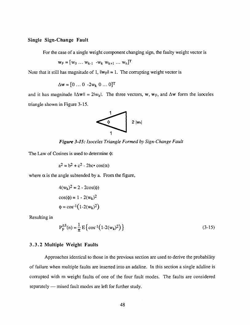
For the case of a single weight component changing sign, the faulty weight vector is
WF = [W0 ... Wk-1 -Wk Wk+1 ... Wn]T
Note that it still has magnitude of 1, IIwFlI = 1. The corrupting weight vector is
Aw = [0 ... 0 -2wk 0 ... 0]T
and it has magnitude IIAwll = 2 1Wkl. The three vectors, w, wF, and Aw form the isoceles
triangle shown in Figure 3-15.
2 Iwk
Figure 3-15: Isoceles Triangle Formed by Sign-Change Fault
The Law of Cosines is used to determine 0:
a2 = b2 + c 2 - 2bc* cos(o)
where c is the angle subtended by a. From the figure,
4(wk) 2 = 2 - 2cos(4)
cos(O) = 1 - 2(wk) 2
S= cos-1(1-2(wk)2)
Resulting in
PF (n)= E cos-1l(1-2(wk) 2) } (3-15)
3.3.2 Multiple Weight Faults
Approaches identical to those in the previous section are used to derive the probability
of failure when multiple faults are inserted into an adaline. In this section a single adaline is
corrupted with m weight faults of one of the four fault modes. The faults are considered
separately - mixed fault modes are left for further study.
Single Sign-Change Fault

As in the previous section, the task is to determine the angle, 4, between the original
weight vector and the faulty weight vector. For a single fault, 4 is a function of wk, 4 = g(wk),
where wk is a single weight component. In the case of m multiple faults, 0 = g(wkl, Wk2, ...
wkm), where wkj are m different weight components. In the general case, the value of 0 is not
dependent upon which weight components have been corrupted, but rather the number of
weight components (m) which have been corrupted. For mathematical uniformity and clarity,
the faulty weight vector will be assumed corrupted in its first m terms, that is, the elements wo
... wm-1 will be considered to be the faulty components.
As before, the weight vector is assumed normalized, Ilwli = 1, and a corrupting weight
vector Aw is defined as Aw wF - w. The derivations mimic the procedures of §3.3.1.
Also, the same arguments for the equivalence of P (n) and P• (n) apply to P (n,m)
and PF (n,m). For those reasons, the two multiple rail fault cases are condensed to one,
denoted P+-(n,m) and assigned, arbitrarily, to the form of P (n,m):+M d+M a (n,m)(
P (n,m) PF (n,m) = PFM(n,m) (3-16)
Multiple Zeroed-Weight Faults
For m zeroed-weight faults, the faulty weight vector is
wF= [0 ... 0 Wm wm-+l1 ... Wn]T
so that Aw - [-wo -W 1 ... -Wm_1 0 0 ... 0]T
Again, WF and Aw are perpendicular, so
IlAwilsin 4 - IIwil
which reduces to
m-1
sin = j(wi)2i=O0
so that

m-1=sin-1 j(wi)2 1/2(i=0
and
POMF (n,m) = E sin-1 IM w i2) 1 /2 } (3-17)
Multiple ±1 Rail Faults
The equation for multiple ±1 rail faults was assigned to the form of the PF (n,m), that
is the form for the multiple +1 rail faults. In this case
WF = [1 1 ... 1 wm Wm-+l ... Wn]T
and the angle between w and WF is found from their dot product:
C os- W WF) =COS lw IWIIIIWF)
= cosI-( Wm (W) 2 (Wm+) 2 ...
+ (Wm) 2 + (Wm+) 2 + ... + (Wn)2) 1/ 2
But from eq. (3-9)
(3-18)
m-1 n(wi)2 + Z(wi)2 = 1
i=O0 i=m
n m-1X(wi)2 = 1- (wi)2i=m i=O
and eq. (3-18) becomes
m-1mwi +
Co - i=O -
v+1-
m-11 - (wi)2
m-1 12j(wi)2 /
i= 0
resulting in

m-1 m-1 "
1wi + 1 - (wi)2PF (nm) = E cos •1 i= i=0 1/2 (3-19)
m + 1 - (wi)2i-0
Multiple Sign-Change Fault
As with the single sign-change fault, the faulty weight vector has unit magnitude,
WF = [-WO -w 1 -... -wm-1 Wm Wm+l ... Wn]T
and the corrupting vector Aw is
Aw = [-2wo -2wl ... -2wm-1 0 ... 0]T
with magnitude
m-1IlAwl = 2 E(wi)2
i= 0
Again the vectors w, WF, and Aw form an isoceles triangle with two sides equal to unity.
Using the Law of Cosines,
m-1IIAwil =4 X(wi)2 = 2 - 2cos(O)
i=O0
so that m-1S= cos-1 1 - 2 (wi) 2
i-0
resulting in
ASM1F ( m-iF (n,m) = E cos-1 1 - 2 (wi)2 (3-20)
i-0
Notice that if all vector components change sign, that is, m = n+l, PF = 1. This is sensible: if
all weights change sign, the weight vector reverses direction. It creates the same decision
hyperplane but reverses the classification of all input vectors.

3.3.3 Summary of Model Equations
The table below, Figure 3-16, provides a summary of the formulas for the four failure
models considered in this section.
Failure Model Notation Formula
Single Zeroed-Weight FaultProbability an adaline misclassifies 0 1 E .sin - 11w k }given one of its input weights, wk, PF(n)has been forced to zero.
Single Rail Fault) 2 +Probability an adaline misclassifies P (n) COS-1 1 (wk)2 kgiven one of its input weights,wk, F X (2 - (wk)2 1/2
has been forced to ±1.
Single Sign-Change FaultProbability an adaline misclassifies AS 1 E t cos-1(1-2(Wk) 2)
given one of its input weights,wk, F (n)changes sign, Wk, -4 -Wk.
Multiple Zeroed-Weight FaultProbability an adaline misclassifies OM (nm) E sin-1 (W)2 /given m of its input weights have F 7 i--0been forced to zero.
Multiple Rail FaultProbability an adaline misclassifies P • nm)given mrn of its input weights have F (nm) 1been forced to ±1. 71
I
1wi + 1 -)
m-]
+1-i---O
Multiple Sign-Change Fault -1 1iProbability an adaline misclassifies ASM = E cos-1 1 - 2 (w)2given m of its input weights change PF (n,m) i=sign. I
Figure 3-16: Summary of Formulas for Failure Modes

The probabilities of adaline failures derived for the various fault modes in the previous
section all involve expected values of functions of the adaline weights. To evaluate the failure
probabilities, the probability distributions of the weight components must be determined. More
specifically, the probability density function of the weight components must be derived.
The adaline weight vector has n+l dimensions, w = [wo w, ... wn]T. If each
component can take on any value, determining probability distributions for the general case is
an intractable problem - specific statistics of the weight vector must be provided. However,
as discussed in §3.3, normalization of the weight vector to unit value has no effect on the
adaline decision function, yet limits the range of vector components. Furthermore, a
normalized weight vector was used to derive the equation for adaline probability and so must
be used here as well. Thus, for the analysis here, w is assumed to be normalized to unit value,
that is:
11wl 2 (w 0)2 + (W1 )2 + ... + (wn) 2
n= (wi)2 = 1 (3-21)
i=O0
Eq. (3-21) is also the equation of a unit hypersphere. Normalization of w to unit length
requires it to lie on the unit hypersphere.
Since the vector represents the statistical information of the input classifications, the
values of each component are highly dependent upon the classification function. The analysis
in this thesis is intentionally general1 2 , so the vector must be considered "randomly oriented";
that is, the vector is assumed to be equally likely to be pointed in any direction. Thus, w is
distributed on the unit hypersphere such that the probability that it lies on any patch of the
12. For specific cases where the weight probability distributions may be known, those distributions can be usedto solve the equations of PF. If the specific weight vector is known, the lune magnitude 0 can bedetermined for all cases and the mean value of 0 should be used for E [ }.
3.4 WEIGHT DISTRIBUTIONS

The vector components wi, i = 0, 1, ..., n, are each dependent random variables on the
interval [-1, +1], with eq. (3-21) imposing the interdependence. Evaluation of the equations
for PF thus requires evaluation of the expected value of functions of random variables. The
expected value of any function of random variables g(xI, x2, ... , xn), where xi are the random
variables, can be determined using the joint probability density function of the random
variables:
E { g(xl, x 2 , ... , Xn)} =
Jg(x 1 , x2, ... , xn) fxIx2...x,(X 1, x2, ... , xn)dxidx 2... dxn (3-22)
where fxlx2...x,(xl, X2, ... , xn) is the joint probability density function 13 and Ox is the range of
the random variables. The expected value of a function of only one random variable g(x) is
simply given by
E { g(x)} = Jg(x)fx(x)dx (3-23)K~x
where fx(x) is the probability density function of x.
The equations for the probability of failure of an adaline with only one fault require the
evaluation of the expected value of a function of one random variable, wk. Those cases can be
solved using eq. (3-23) and the probability density function for wk. The equations for the
probability of failure of a multi-fault adaline require that the joint probability density function of
wo, wl, ... , wm-1 be used in eq. (3-22). In this section, these probability density functions are
derived.
Thus the problem is: given an n-dimensional1 4 random vector w = [wl w2 ... Wn] T
distributed uniformly over the unit hypersphere, determine the probability density function of a
dFx(x)13. Notation based loosely on Drake [14]. Fx(x) = P{x <: x}; fx(x) - dx)
14. This can obviously be extended to the n+1 dimensional vector w = [wo W1 ... wn]T.
hypersphere is equal for equally-sized patches.

single vector component wi, denoted fw(w), and the joint probability density function of m
components Wl, w2, ... , Wm, denoted fw(Wl...Wm). Because fw(w) is a special case of
fw(wil...wm), i.e., fw(w) = fw(wl...wm) for m = 1, fw(wl...wm) is first derived.
The key to deriving the probability density function is to properly interpret the meaning
of the vector being "distributed uniformly over the unit hypersphere." Since the goal is to have
all directions equally likely, patches on the unit hypersphere of equal surface area (technically,
of equal surface "content" [48]), must be equally likely to contain the vector. Patches of
unequal area will have unequal probabilities of containing the vector and the ratio of those
probabilities will be equal to the ratio of the surface areas.
The probability that the vector lies on the patch which covers the entire hypersphere is
clearly unity. So, the probability that the vector lies in a smaller surface patch of area ds is
simply the ratio of ds to the surface area of the hypersphere:
dsProb{wo < W Wo + Aw} = (3-24)
Sn
where wo is an arbitrary vector, Aw is an incremental vector, such that both wo and wo + Aw
meet the constraints of eq. (3-21), ds is the surface area of the patch subtending Aw, and Sn is
the surface area of an n-dimensional hypersphere. Sn is readily available 15 [41, 48]:27t n /2
Sn 2- /2 (3-25)
where F(y) is the gamma functionl6:
15. The meaning of the term Sn varies by discipline. For this thesis, Sn will denote the surface area of the unithypersphere which occupies n-dimensional space. For example, S3 is surface area of the conventionalsphere. It has surface area, from eq. (5-25), of S3 = 47r. Mathematicians [41] often denote the surface areaof a hypersphere which occupies n-dimensional space as Sn-1, since the surface is a manifold of n-1dimensions in 9S n. Of course the area is the same; only the notation and formula for Sn are different.
16. Three important properties of the gamma function are useful for evaluating ( ) [03370]:
F(x) = (x-1)!, for x an integer; F( = ; and F(y+1) = yF(y).(2Fnd]x) =) F~ )

1
F(y) = xy-le -x dx (3-26)0
Equation (3-24) is the essence of the derivations to follow.
A note on symmetry is in order before the density functions are derived. Since the
hypersphere is symmetrical in all directions and the components of w are numbered arbitrarily
(or, the axes of in are labelled arbitrarily), the probability density function for the single
vector component is independent of the particular component chosen. Thus, fw(w) will be
identical for all components. Similarly, the joint probability density function for the first m
elements is identical to the joint probability density function for any m elements. The
recognition of the equivalences of these functions simplifies the derivations.
3.4.1 Joint Probability Density Function of Several Weights
As stated in eq. (3-24), the ratio of the surface area of a "patch" on the unit hypersphere
to the total hypersphere surface area is the probability that a unit vector distributed uniformly
over the hypersphere lies in that patch. For a patch which subtends only differential elements,
the surface area ratio gives a probability density function. For a patch which subtends m
differential elements, a joint probability density function of m components is found. (For m =
1, the single probability density function for one component is found.) Finding the probability
density functions thus requires finding the surface area of the "patch".
By definition, the probability that the vector w lies in a patch which subtends m
differential components is the joint probability density function times the differential area of the
subtending components:
w < w 1 • w 1 + dw1
Prob w2 < W 2 W2 + dw 2 = fw(W1.. .Wm) dwl dw2 ... dwm (3-27)Wm < Wm < Wm + dwm
The probability is also equal to the ratio of the surface area of the patch to the surface area of
hypersphere, eq. (3-24):

10
ýnsubtending patch on hypersphere,area ds
dw
dwi... 00 ,differential components,
in general, dwl dw2 ... dwm
Figure 3-17: Patch of Area ds Subtending m Differential Components
Determining the patch area requires considering the higher order space 9Sn . Excellent,
if dated, texts are available on the subject [48, 68], but by decomposing the space into smaller
dimensional spaces which can be more easily expressed, the patch area can be described here.
The n-dimensional space 9gn is spanned by the unit vectors u I, u2, ... , Un. This space
can be considered as two orthogonal spaces, one spanned by ul, u2, ... ,Um, and the other
spanned by Urn+1, Um+2, ... , Un. This is shown in Figure 3-18, with a horizontal vector x =
111 + u2 + ... + um and a vertical vector y = um+1 + urn+2 + ... + Un. In this depiction, the
unit hypersphere filling 91n is a 2-dimensional circle, as shown, with radius r = 1. The vector
w must lie on that circle; it too can be decomposed into w = wx x + wy y.
A patch on the unit hypersphere which subtends m differential components dwl, dw2,
... dwm at wx, as shown in Figure 3-19, has an m-dimensional arc length da. The area of the
w , < wl < w, + dw 1
Prob •w2 < W2 W2 + dw2 s (3-28)... Sn ( -8wm< Wm< m + dwm s
where ds is the area of the patching subtending dwl dw2 ... dwm. Equating the right sides of
the above probabilities,ds
fw(wl...Wm) = Sn dw1dw 2 ... dwm (3-29)
The problem is now to determine the ds, the area of a patch on a unit hypersphere which
subtends m differential components. Figure 3-17 provides an illustration.

X = Ul+U2+...+Um
Figure 3-18: Unit Hypersphere in a Simplified 9n
patch, ds, is equal to the arc length times the area, A, of the underlying surface.
ds = da * A (3-30)
That underlying surface spans the remaining n-m dimensions and has dimension n-m-1 (n-m-1
degrees of freedom). The patch will have dimension n-1; m dimensions from da and n-m-1
dimensions from A.
Wy
Figure 3-19: Patch Arc Length, da
To understand the meaning of eq. (3-30), consider Figure 3-19 as a cross-section of a
conventional 3-dimensional sphere. The area of the patch which subtends a single differential
component dx at wx is the arc length da above wx times the circumference of the circle at wx
which is perpendicular to x. The "circumference of the circle" is simply the "area" of the
y = Um+l+Um+2+...+Un

underlying surface which spans the other 2 dimensions. Here, m=l1, so the arc length has
dimension 1 and the underlying surface has dimension 3-1-1 = 1 as well. The patch itself has
dimension 2: it is a differential ring.
The first step is to find the arc length da. From Figure 3-19, the relationship between
da and dwl dw2 ... dwm can be directly determined:
dwIdw2 ... dwmda = sin0 (3-31)
where 6 is the angle between w and x. But,
sine =_yIIwiland since I4wl- = 1,
sin0 = wy (3-32)
Now, wx is the length of the first m components of w:
mwx = (wi)2 (3-33)
i=1
by using IIwlI = 1 and Pythagoras
wy 1 - (wx) 2
m= 1 - (wi)2 (3-34)
i= 1
Combining eq. (3-31), (3-32), and (3-34), yields an equation for da:
da = dwIdw2 ... dwm (3-35)< rn
1 - (wi) 2
i=1
Although the patch will always subtend dwl dw2 ... dwm, it will also span a surface
over the remaining n-m dimensions. To see this, expand the 2-dimensional depiction to 3
dimensions, one spanned by ul, U2, ... , um as before, one spanned by only Um+1, and one
spanned by the remaining unit vectors, Um+2, um+3, ... , Un. Define the spanning vectors x =

Ul + u2 + ... + um, y = Um+1, and z = um+2 + um+3 + ... + Un, shown in Figure 3-20. Asbefore, w can be decomposed into w = wx + wm+1y + wzz.
+Un
y = Um+1
Wx
X = Ul+U2+...+Um
Figure 3-20: 3 -dimensional Depiction of the Hypersphere Slice in 9?n
The differential slice in Figures 5-18 and 5-19 becomes a differential ring in Figure 3-20. It has a radius, r, equal to distance between the arc da and x. From Figure 3-19,
mr = wy = 1 - (wi)2 (3-36)
i=1
To see this formally, remember that the vector w = wxx + wm+ly + wzz must alwayssatisfy the equation of the unit hypersphere:
nn(wi) 2 = 1
i=1
which expands tom nj(wi)2 + (Wm+1) 2 + X(Wi)2 = 1 (3-37)i=1 i=m+2
m nbut (wx) 2 = (wi)2 and (wz) 2 = (wi)2, so eq. (3-37) becomes
i=1 i=m+2
(wx) 2 + (wm+1) 2 + (wz) 2 = 1
or (wm+1) 2 + (Wz) 2 = 1 - (Wx) 2 (3-38)
For a fixed wx, eq. (3-38) has the form of an equation of a circle in the y-z plane:
(wm+1) 2 + (Wz) 2 = r2

Thus, at a fixed wx the surface of the hypersphere is a circle parallel to the y-z plane, centered
on the x axis with radius r,
r = 1i - (wx) 2 , or
or r = 1 - (wi) 2
i= 1
which is eq. (3-36). Of course, the surface is a circle because only 2 dimensions, y and z, are
depicted. In the vernacular of higher geometry, a circle is a hypersphere of 2 dimensions.
To go beyond 2 dimensions and obtain the general surface of n-m dimensions, eq.
(5-38) is re-expanded with r given by eq. (3-36):
(wm+1) 2 + (wm+2) 2 + ... (Wn) 2 = r2 (3-39)
This is the equation of an n-m dimensional hypersphere with radius r. Thus, the surface
spanned by the remaining n-m components of w is an n-m dimensional hypersphere withm 12
radius given by eq. (3-36), r = 1 - , (wi)2
i=1
As stated by eq. (3-30), the area of the patch subtending m differential components is
the m-dimensional arc length, da, times the area of the underlying (n-m)-dimensional
hypersphere, A. Using the 3 dimensional sphere as an example again, the patch above a single
differential component dwl at wi is a differential ring with area equal to the arc length times the
circumference of the ring at wl, shown in Figure 3-2117. The "circumference of the ring" is
technically the area of a 2-dimensional hypersphere.
The surface area of n-dimensional hypersphere with a radius other than unity, denoted
An, is given by [48]:
17. In this case, da = dw and the circumference = 2nr, r = 1-(wl) 2 . Thus, the area of the patch is the
constant 2ndw. This interesting well-known result [53] reveals that if a sphere is sliced into equal widthsperpendicular to one axis, each slice will have equal surface area. For example, an orange cut up in such away would yield slices with equal peel area.

r2=_=1X1
2
Figure 3-21: Slice of a Sphere at One Fixed Component, wj
An = Sn rn-1(3-40)
where Sn is the surface area of the unit n-dimensional hypersphere, given by eq. (3-25). The
area of the underlying (n-m)-dimensional hypersphere with radius r given by eq. (3-36) is thus
ASnmm n- )/(wi)2 2A = Sn-mn 1-1(wi)2i=1 I
(3-41)
Combining this result with length of the arc da, eq. (3-35), the area of the patch is
finally obtained:
m =wwn-m-1)/21- (wi)2
ds = dwidw2 ... dwm Sn-m (=m 1/2
1-1(wi)2
i=1
which reduces to
ds = dwldw2 ... dwm Sn-m m n-m-2)/21-1(wi)2
i=l(3-42)
The patch area is substituted into eq. (3-29) to obtain the joint probability density
function:
dwidw2 ... dwmm n-m-2)/2
Sn-m 1 - E(wi)2i=l1
fw(wil...wm) dwldw2...dwm Sn

which simplifies nicely to
S. Sn-m- 2)/2
f(wl...wm) = Sn -I (wi) 2 (3-43)ni=l1
SnmUsing eq. (3-25), the fraction n is reduced for easier computation:Sn
F(2) m n-m-2)/2
fw(wil...wm) = nm()m/21- (wi)2 (3-44)
Behavior of the Joint Probability Density Function
With the joint probability density function in hand, some comments on its behavior are
in order. First, note that despite its complicated form in eq. (3-44), the function of eq. (3-43)
is actually quite elegant. It reveals that the joint probability density function of m components
is given by a constant term times the radius of a particular hypersphere raised to a power. The
constant is the ratio of the surface area of an (n-m)-dimensional unit hypersphere, Sn-m, to them 1/2
surface area of an n-dimensional unit hypersphere, Sn. The radius, r = 1-(wi)2 , is thati=l1
of an (n-m)-dimensional hypersphere on the surface of the n-dimensional unit hypersphere.
The power (n-m-2) is simply two less than the difference in dimensions.
A relevant question is the validity of the form of eq. (3-43) when m=n; can the joint
probability density function of m components be used to determine the probability density
function of all n components? The answer is yes, with some appropriate interpretation.
First the density function of eq. (3-43) must be formally stated to account for the
constraints on the range of the components. Formally, the probability density function is non-
zero only when the components are within the n dimensional unit hypersphere:

miff (wi) 2 < 1
i=1
0 otherwise
For m=n, the density function is non-zero only when the components are within the n-
dimensional unit hypersphere1 8 . From eq. (3-45),
SoSnSn 1- (wi)2
0
niff (wi)2 < 1
i=1
otherwisen
Now, So = Ot, so fw(wi...wn) = 0, unless (wi)2 = 1, in which case the denominator of eq.i=1
(3-46a) is zero as well. But, this condition holds in all cases: it is the requirement of w being an
unit vector. Cancelling the zeros in the numerator and denominator at E(wi)2 = 1, eq. (5-46)i=1
becomes:
fw(wl...wn) =
1Sn
0
n
iff (wi)2 = 1i=1
otherwise
Eq. (3-47) states that the n components of a unit vector are simply distributed uniformly over
the surface of the unit hypersphere - which was the original statement guiding the derivations
of this section. The Sn in the denominator is a normalizing factor so that the density over the
surface integrates to 1.
18. The components must actually be on the n-dimensional unit hypersphere. This condition is met by theresulting equation.
t S o = 2 and 0.F(0) F(0)
(3-46a)
(3-46b)
(3-47)
) m n-m-2)/2(f Sn-m m nSn 1 - (wi)2fW(wi ... W.) = nI=1 (3-45)
fw(Wl...Wn) =

I I1 iffw 12 + w 2
2 = 1
fw(wiw2)= Sn - 2n
0 otherwise
The density is illustrated in Figure 3-22. It is an infinitesimally thin, hollow cylinder of radius1
1 and height 2~, centered at the origin. The "area" under the density (which must equal 1) is1
simply the circumference of the unit circle times the height of the cylinder: 2n = 1.
At £ i -.. .. .
W2
Figure 3-22: Joint density of Both components of a Vector on the Unit Circle
The density for a single component can be determined by integrating out the density of
the other component. The area under the density contributed by w2 for each dw, is 2da times1
the height 2, where da is the arc length at w, shown in Figure 3-23. From Figure 3-19,27,dw
da dw=
1so fw(wi) = 1
which agrees with eq. (3-43) for n=2 and m=l.
It is often instructive to study the behavior of a probability density function by
identifying its first two central moments, i.e., its mean and variance. Since eq. (3-43) is an
even function of all of its arguments, all variables have zero mean. This reduces the covariance
matrix to
For example, for n = 2:
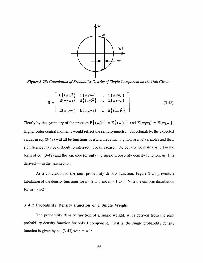
'4k W2
-J
da
q
W1
dwi
Figure 3-23: Calculation of Probability Density of Single Component on the Unit Circle
SEt(wa)2) E{waw 2} ... E{WiWm)} 1R= E{w2W1} E{(w 2)2} ... E{w 2Wm} (3-48)
LE{wmwl} E{wmW2 ) ... E t(wm)2I
Clearly by the symmetry of the problem E t (wi) 2 } = E t (wj) 2 } and E {wiwj I = E { wkWl I.
Higher order central moments would reflect the same symmetry. Unfortunately, the expected
values in eq. (3-48) will all be functions of n and the remaining m- 1 or m-2 variables and their
significance may be difficult to interpret. For this reason, the covariance matrix is left in the
form of eq. (3-48) and the variance for only the single probability density function, m=1, is
derived - in the next section.
As a conclusion to the joint probability density function, Figure 3-24 presents a
tabulation of the density functions for n = 2 to 5 and m = 1 to n. Note the uniform distribution
for m = (n-2).
3.4.2 Probability Density Function of a Single Weight
The probability density function of a single weight, w, is derived from the joint
probability density function for only 1 component. That is, the single probability density
function is given by eq. (3-43) with m = 1:

19. Although the ratio appears reducible, because n is an integer the function can be calculated
relatively easily and the fractional form is easier to use than a reduced form. Appendix B.1 derives a formfor the ratio which does not explicitly require the gamma function. For notational convenience, the originalfractional form will be used.
Snm m n-m-2)/2fw(Wi...Wm) = 1- (wi)2
i= 1nn
mn 2 3 4 5
1 1 1 2 3 1(W
( 2 2 (w1)2 4 ((wlY 2)
2 1 1 1 3 1-(w)2 2
27r 2r 1-(w1)2-(w2)2 27r
3 1 2 3- 47 1-(w )2- 2) 2 47c
4 1 321r2 47t 2 1-(wl)2_(w2)2-(W3 )2(w4)2
5 387r
2
Figure 3-24: Tabulation of Joint Density Function
fw(wl) = 1 1X wi2 n-3)/2i=l1
which, after dropping the subscript on w and simplifying the notation, becomes
fw(w) = 2()_ _(1-w2)( n-3)/2 (3-49)
The distribution is an even function with zero mean and, except for the case of n=2, a
mtntmaximum value (at w = 0) given by the ratio19 12;

It is instructive to see how f,(w) behaves as n grows large. Because the sum of the
squares of the components must equal 1, it seems likely that the probability density function of
any component will be amassed near 0 for large n. That is, it is unlikely that the component
takes on a value near 1 since all other components must then be much less than 1 but all have
identical probability distributions.
Indeed, this is the case. The value of increases with n. The variance,
1calculated in Appendix B.2, is given simply by 1 .
The equations of fw(w) for various values of n are tabulated in Figure 3-25. The actual
distributions are plotted in Figure 3-26.
3.5 PROBABILITY OF ADALINE FAILURE
Evaluation of the probability of adaline failure requires the incorporation of the
probability density functions derived in the previous section into the formulae for the
probability of the adaline failure from §3.3. Those results are repeated here for convenience.
PF(n) =1 E t sin-I1wkI } (3-50)
XE1 1 co( 1-2 (Wk) 2 + wk'(
PF (n)=E cos= 1 2)1 2k (3-51)X (2 - (wk)2)l/2 )
PF AS(n) 1 E cos-1(1-2(wk) 2) } (3-52)
PF (n,m) = -E sin--1 wi) 2 1/2 (3-53)
m-1 m-1 "wi + 1 - y(wi)2
+M 1 i_-0 i-0PF (n,m) = E cos-1 1 1/2 (3-54)
m + 1 - (wi)2j
q i=_0

f ,w)
-1 -0.5 0.5 1
Figure 3-26: Probability Density Function for Values of Vector Dimension, n
20. The result for n=2 agrees with the result conventionally derived when w is one of the two vectorcomponents on the unit circle [34]. Note that despite the fact that fw(1) = oo, there are no impulses at w = 1and therefore the probability of w =1 is zero. A similar phenomenon occurs in all cases of the joint densityfunction when m = n - 1.
21. For n=3, the uniform distribution is a well-known paradigm; see note 17.
nI2nm2
n fw(w) n fw(w)1,
2(see note 20) 20 1.72(1-w2) 8 .52 lcw2(sent20
31 (see note 21) 50 2.78(1-w2) 2 3 .5
2
4 2 . 12 100 3.96(1-w2) 48.5
5 (1-w2) 500 8.92(1-w2) 298 .5
10 1281 2 7/2 1.16(1-w2) 7/2 1000 12.6(1w2) 4 9 8 .5
Figure 3-25: Tabulation of Single Probability Density Function

PASM, .PF (n,m) =1 m-1
E cos -1 1 - 21(wi)2i= 0
Recall that for notational convenience, the density functions of §3.4 were derived for an
n-dimensional vector, w = [Wi w2 ... wn]T. The weight vector of interest, however, has n+l
elements, where n is the number of true adaline inputs, w = [wo wi ... Wn]T. Thus, the
density functions for the weight vector of an adaline with n inputs are:
F n+1'
fw(w) = (l-w2)(n-2)/2
fF(n+l)\(fw(wl...wm)
(2
i[- (n-+)7)m/2
(3-56)
m-1 n-m-1)/2(wi)2
i=0O(3-57)
The problem is now to use eq. (3-22) and eq. (3-23) to solve eqs. (3-50) through (3-55). In
Ead}all cases, P = and ( = g(wo,... ,wm-,n), so
1PF(n) = 1 fg(w,...,w.,n) fw(w,...,w
PF(n) = x- Jg(wo,...,wm-l,n) fw(wo,...,wm-1)dwo...dwm-1 (3-58)
The particular instantiations of eq. (3-58) are as follows:
] ((n+(1) 1
PF (n )t3/2 _Jsin-lwl (1-w 2 )(n-2)/ 2dwF 2 1 321) 1
(3-59)
( - n +2 )p 1 (n)= 2(
F 2!3/2cos-
-1
)2+1(1 - (w) 2 + w 1-w2)(n-2)/2dwS(2 - (w)2)1/2
F(n+1 1
PFAS (n) = ()2 cos-1 (1-2(w)2) (1-w2)(n-2)/2dwF( Q!>3/2 1
(3-60)
(3-55)
(3-61)
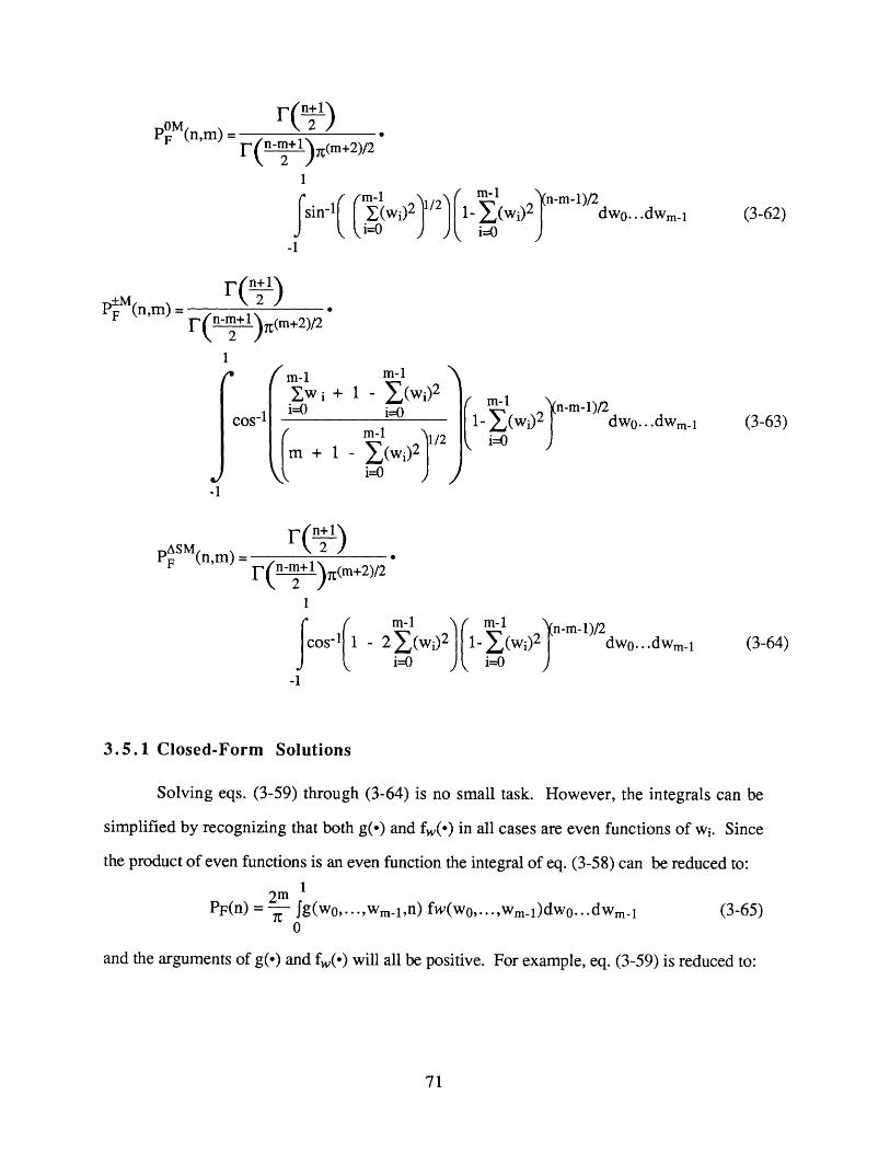
rQ(n+1nM )2POF (n,m) = 2
F(2 )g(m+2)/2
1-I
i=0dwo...dwm.-1
F~2V2)g(m+2)/2
m-11 - (wi)2
i=0O Cm-1 1/2
Y(Wi)2i=O
m-11- (wi)2i=0
dwo...dWm-l
rp(n-n+i )7(m+2)/2
(m-1 m-1lcos -1 1 - 2X(wi)2 1-Y,
i-0 i=0-1
(wi)2n-m-l)/2
dwo...dwm-1
3.5.1 Closed-Form Solutions
Solving eqs. (3-59) through (3-64) is no small task. However, the integrals can be
simplified by recognizing that both g(-) and fw(*) in all cases are even functions of wi. Since
the product of even functions is an even function the integral of eq. (3-58) can be reduced to:1
2mPF(n) =1 fg(wo,...,wm_l,n) fw(wo,...,wm_l)dwo...dwm-1l
and the arguments of g(o) and fw(*) will all be positive. For example, eq. (3-59) is reduced to:
+MPF (n,m)
Sn-m-1)/2(3-62)
} (n-rn-i)/2
ASMPF (n,m)
(3-63)
(3-64)
1Isin-1( 1(mwi)2 : 2
i= 0
-
9V(3-65)

S 2mF n+) 1P (n,m) = 2 J sin- 1(w)(1 -w2 )(n- 2)/2dw (3-66)F (!01 3/2 0
Further simplifications can be made by recognizing similarities in the arguments of g(*) and
fw(.) and making clever substitutions.
Despite these simplifications, the integrals are still formidable. Closed-form solutions
are attainable, but those forms themselves are complicated functions which are impractical to
solve by hand. The single zeroed-weight fault, for example, has the simplest integral to solve,
eq. (3-66). That integral can be reduced to
2m]F n+1 IP 2mF( ) (2) sin- (w)(1-w2)(n-2)/2dwPF(nm) 2 n)t3/2 0
2mF n+1 i/2- J2O(cos) n-3dO (3-67)]F ,3/2 0
The solution to equation (3-67) derived in Appendix B.3, is non-trivial.
Because the integrals reduce to a form impractical to solve by hand for any reasonably
large n, the formulas for the probability of adaline failure are left in the forms of eqs. (3-59) to
(3-63). Several computer-aided techniques, including simulation [44], or mechanical
quadrature [27] can be used to determine PF(n,m) for particular values of n and m.
3.5.3 A Monte Carlo Simulation
Instead of integrating the equations (3-59) through (3-64) and solving for the PF
directly, the trend for the failure probabilities as functions of n and m are determined. This is
accomplished through simulation of statistical trials, the so-called Monte Carlo method [44]. In
this process, N vectors, xj, j =1... N, with distributions identical to the distributions of the
adaline weight vector are constructed. The value of Pj = g(xj) is then calculated. For large
enough N, the average value of 0 approximates its expected value. That is, according to the
Law of Large Numbers
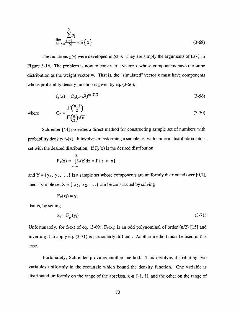
N
rN=E{( o (3-68)N~*0
The functions g(*) were developed in §3.3. They are simply the arguments of E{*} in
Figure 3-16. The problem is now to construct a vector x whose components have the same
distribution as the weight vector w. That is, the "simulated" vector x must have components
whose probability density function is given by eq. (3-56):
fx(x) = Cn(1-x2)(n-2)/2 (3-56)
where ( )Cn = (3-70)wher Cn i.,2)_ -
Schreider [44] provides a direct method for constructing sample set of numbers with
probability density fx(x). It involves transforming a sample set with uniform distribution into a
set with the desired distribution. If Fx(x) is the desired distribution
x
Fx(x) a ffx(z)dz = P{x < x}- 00
and Y = {y 1, Y2, ... } is a sample set whose components are uniformly distributed over [0,1],
then a sample set X = { x1, x2, ... } can be constructed by solving
Fx(xi) = yi
that is, by settingF-1
xi = F (yi) (3-71)x
Unfortunately, for fx(x) of eq. (3-69), Fx(xi) is an odd polynominal of order (n/2) [15] and
inverting it to apply eq. (3-71) is particularly difficult. Another method must be used in this
case.
Fortunately, Schreider provides another method. This involves distributing two
variables uniformly in the rectangle which bound the density function. One variable is
distributed uniformly on the range of the abscissa, x e [-1, 1], and the other on the range of

the ordinate, y E [0, max(fx(x))]. A test is performed on the pair (x,y): if y < fx(x), then the
variable x is placed in the sample set. Otherwise the pair is discarded. The process is repeated
until the desired sample set size is obtained.
The process is illustrated in Figure 3-28, with fx(x) from eq. (3-69) with n=100. For
pair A, yl < fx(xl), so xl is saved for the sample set. But, for pair B, Y2 > fx(x2), so the pair
is discarded and x2 is not placed into the sample set. If a large number of pairs is generated,
the points (xi,yi) will be uniformly dispersed in the rectangle ([-1,+1], [0,Cn]). The process
will bias the X sample space; the bias is determined by the probability density function.
f '(x)
x-1 Xl X2 +1
Figure 3-28: Process for Creating Biased Sample Space
To code the process for simulation, a pair of random numbers is created. The variable
x is distributed uniformly between -1, and +1. The variable y is distributed uniformly between
0 and Cn, where Cn is given by eq. (3-70). If y • Cn(1-x 2 )(n-2)/2, then the variable x is written

to a file representing the sample space. 22 The process is repeated until the sample space is
adequate in size.
Monte Carlo simulations were used to estimate adaline failure probability for all of the
fault modes previously discussed. To ascertain a trend for likelihood of adaline failure as the
number of inputs grow, simulations for n=10, 20, 30, 40, 50, 100, 200, 300, and 500 were
performed. For the multiple fault cases, faults were inserted as a percentage of the number of
inputs. Three cases were simulated: 1% faulty weights, 10% faulty weights, and 50% faulty
weights23 . For n < 100, the 1% faulty weights case was omitted. The following procedure
was used for each case of n:
1. A 100,000 element sample set was created. The elements have a
distribution equivalent to components on an n+ 1 dimensional unit
hypersphere (density of eq. (3-56)). The sample set was created using the
process described by Figure 3-28.
12. For the single fault case, where PF(n) == Efg(w)}, Pr was determined as
the average of all 100,000 components processed by g(*):
1 1 100,000PF = i 100,000 1 g(xj)
j=1
As a sanity check on the sample set, an average sum of squares for n+1
components was also taken. Ideally this should be equal to 1.
3. For the multiple fault case, m elements were randomly selected from the
sample set and processed by g(o). The adaline failure probability was
estimated as the average of 100,000 of these trials:
22. A coding simplification can be made by eliminating the factor Cn. For y distributed uniformly on [0,1] and
a test of y < (l-x2)(n-2)/2 , the same results will be obtained. Elimination of Cn simply scales the densityfunction and the Y sample space both to 1.
23. More accurately the cases were, m=0.01n, m=0.10n, and m=0.50n. The number of inputs is n, but anadaline has n+1 weights.

1 1 100,000PF = 100,000 1 g([wow1 ... Wm]j)
j= 1
where [WOWl ... Wm]j is a set of m randomly selected elements from the
sample space.
The size of the sample space, or more specifically the number of trials, in a Monte
Carlo simulation determines it accuracy. From the Chebyshev Inequality, the accuracy of a
Monte Carlo simulation can be determined: for N trials, the error in predicting an event
probability is inversely proportional to the root of N [44]. That is,
Ng (xj) 1
S=N - E{ g(x)} (3-72)
For the simulations here, 100,000 trials were performed, resulting in an error = +0.003. Thus
the results for the adaline failure probability can be assumed accurate in the second decimal
point.24
The procedure enumerated above provides a quick survey into the trend for adaline
failure probability. It suffers, however, from an important statistical inaccuracy: the
components on the n-dimensional vector are independent. Ideally, n components should have
some measure of dependence upon one another, because in fact they are dependent random
variables. A more rigorous method for creating a sample space would be to create m
components at a time using the multi-dimensional joint probability density function, eq. (3-44).
In this method, m components, xi, would be drawn from a uniform distribution over [-1,+1].
An additional element, y, distributed over [0, Cn] would also be drawn. If y • fx(xl, ... , Xm),
where fx(xl, ... , Xm) is the joint density of eq. (3-44), then the m xi components would be
used as a sample. 100,000 samples would be then be averaged.
The problem with this more rigorous method is computation time. For any reasonably
24. Note that 4,000,000 independent trials would be required to secure the third decimal point.

large m, the probability that y < fx(xl, ... , Xm) is very small.25 Some tests using this method
were attempted: tens of thousands of "bad" samples were found for every good sample, when
m was only 20. Computation times of days were required to achieve any reasonable sample
size. A positive note, however, is that the preliminary results showed that the dependent
samples resulted in statistically insignificant differences from the independent samples (see
discussion below).
The source code and results for the simulations are contained in Appendix A. The
following section interprets the results.
3.5.3 Simulation Results
The results of the Monte Carlo simulation are tabulated in Figure 3-29. Plots of the
data are presented in Figures 3-30 through 5-33. This section contains some interpretative
commentary on the data.
The first note of interest is that the sum of the squares for n+l components behavedn
very well. In all cases, I(xi)2 = 1.00 ± 0.009. This means that the simulation did create ai=O0
sample set whose elements have a distribution such that the sum of n+1 squares equals unity,
which was the original intention. That is, the independent trials behaved as if they were
dependent.
25. At a minimum, the sum of the squares of the xi components must be less than one. The sample space isan n-dimensional hypercube of volume 2n. The volume enclosing the elements whose sum of squares isless than 1 is a hypersphere of dimension n and radius 1. Its volume becomes a very small fraction of thevolume of the hypercube as n grows large.

TYPE OF FAULT
n m
110
5
1
20 2
10
1
30 3
15
1
40 4
20
1
50 5
25
1
100 10
50
1
200 2
20
100
1
300 3
30
150
1
500 5
50
250
Figure 3-29: Tabulation of Simulation Results
Sign-Zeroed Rail Sign-
Change
0.081 0.258 0.161
0.235 0.422 0.469
0.057 0.254 0.114
0.090 0.317 0.180
0.0243 0.484 0.486
0.046 0.252 0.093
0.093 0.346 0.186
0.243 0.458 0.488
0.040 0.252 0.080
0.095 0.364 0.190
0.245 0.462 0.491
0.036 0.252 0.072
0.97 0.378 0.193
0.247 0.467 0.493
0.025 0.251 0.051
0.099 0.411 0.199
0.248 0.477 0.496
0.018 0.250 0.036
0.028 0.305 0.056
0.101 0.437 0.202
0.249 0.484 0.499
0.014 0.250 0.029
0.029 0.335 0.059
0.101 0.448 0.202
0.248 0.486 0.497
0.011 0.251 0.023
0.030 0.367 0.060
0.102 0.460 0.203
0.249 0.490 0.498
Sum ofSquares
0.996
0.998
0.991
0.992
0.998
0.997
1.000
0.994
0.995

I-.
"• 0.25U-
._ 0.20(U
0.150
> 0.10
., 0.050
.0.000.00
0 100 200 300 400 500
Number of Adaline Inputs (n)
Figure 3-30: Probability of Adaline Failure for Single Fault Cases
For the single fault case, Figure 3-30 shows that the adaline failure probability
decreases exponentially with n for both the zeroed-weight and sign-change fault modes. Curve
fitting indicates that
0o kPF (n) (3-73)
andPFAS (n) 2k (3-74)
0 A
where k = 0.25. This is a sensible result: PF(n) a E{ sinl(wi)} and P S(n)
Efcos-1(1-2wi 2) j; for wi small, sin-l(wi)= wi, so PF(n) a E{wi}; also for for wi small,
CoS1(-2w2)= sn-(2i) 2i o ASA S 0cos(1-2wi2) sin-(2wi) = 2wi, so P•S(n) aO E{2wi}. Thus, PF (n) = 2 PF(n). This
doubling is also apparent in the raw data (Figure 3-29).
Clearly from the figure, a rail fault is far more likely to cause adaline failure than either
of the other two fault modes. This is because w, the non-faulty weight vector, is normalized to
unit length. For n of any meaningful magnitude, including n =10, the weight components wi
are small. Since the probability of a single rail is given by
0.30

±1 1• -1 (k)2 +WklP (n) = Ecos-1 k (3-14)
with all wk small, PFI(n) - E2cos-1 = 0.25, as indicated.
Interpretation of the multiple fault data is a lesson in asymptotic behavior. This is
because for large m the sum
m-1(wi)2 = m (3-76)
i=O0
For example, for the multiple zeroed-weight fault,
p OM(n,m)= E sin- (wi)2
which for m large, using eq. (3-76), becomes
OM 1 (3-77)PFM(n,m) = - sin -1 (3-77)pOM 1
so PFM (n,0.01n) - sin-1(0.1) = 0.030OM 1
PF (n,0.1n) = sin-1(0.32) = 0.1020M 1
PF (n,0.5n) -= sin- 1(0.707) = 0.250
These results agree with the data for large n.
Similarly, for the multiple sign-change weight fault,
ASM 1 ( rm-iP (nm) = -E cos-1 1 - 2 j(wi)2F 7Cnim ) i=0
which for m large becomes
PF (n,m) = cos(1 - 2) (3-78)
so P ASM(n,0.0ln) = cos-1(0.98) = 0.064
ASM 1PF (n,0.ln) = 1-cos-1(0.8) = 0.205
ASM 1PF (n,0.5n) = - cos-1(0.1) = 0.500
Again, these results agree with the data.

L.voUUe-VVl1FI1L IaUILS -
m=0.5n
m=0.1n
S-.0 M m=0.Oln -
100 200 300 400 500Number of Adaline Inputs (n)
Figure 3-31: Probability of Adaline Failure for Multiple Zeroed-Weight Faults
U- m=0.5n -
0 - m=O.ln
0 m=0.01 n
p--
0 100 200 300Number of Adaline Inputs (n)
400 500
Figure 3-32: Probability of Adaline Failure for Multiple Sign-Change Faults
For the multiple rail fault cases, the asymptote is only clear when m is a large
percentage of n. In this case IIWFII is much larger than w o WF, so the argument of cos- 1(.)(wowF'\
vanishes: - cos-• I-Fwi) and 0 approaches .
U.U -
0.25-
0.20-
0.15-
0.10-
0.05-
0.00
0.6
0.5
0.4
0.3
0.2
0.1
0.0
A --
IRI
A A

0 100 200 300 400 500Number of Adaline Inputs (n)
Figure 3-33: Probability of Adaline Failure for Multiple Rail Faults
3.6 PROBABILITY OF MADALINE FAILURE
Extension of the models for adaline failure to a madaline network can be made by
propagating the adaline failure probability through the network. In this section, a technique is
described for propagating adaline failures. It is based upon the combinatorial probabilities and
utilizes the adaline sign change weight fault model.26
Since a madaline network consists of connected layers of adalines, an adaline failure in
one layer results in an output error which is propagated to the input of the adalines in the
subsequent layer. There is some probability that despite being non-faulty an adaline in the
subsequent layer produces an output different than it would have if all its inputs were correct.
In other words, there is some probability that the "down stream" adalines produce erroneous
outputs and behave as if they have failed. The problem is to determine the probability that
adalines in the last layer - the output layer - produce erroneous outputs.
26. It should be noted that Stevenson [50] developed a different method for propagating failures in a madaline.That method employs an approximation of adaline failure probabilities and is valid when the probabilitiesare small.
0.50_=
" 0.45
. 0.40
' 0.35
0.30
S0.25%2 0.25
n n c se4%1 911

The key to propagating an adaline failure combinatorially through a madaline network is
recalling that the probabilities of adaline failure described previously in this chapter are
conditional probabilities. They stated the probability of adaline failure, or erroneous output,
conditioned on the event that a fault occurred. Furthermore, in §3.1 the assumption was made
that fault-free adalines do not fail. Thus, the unconditional probability that an adaline fails is:
Prob { adaline failure } = PF(n,m) * Prob{ fault occurs } (3-80)
where PF(n,m) is the conditional probability of adaline failure. Figure 3-34 illustrates with a
Venn diagram.
S/PP{S}= 1
F P{EF}= P{EnF}PE P{ F)
P{En rF} = P{E}
E P{E} = P{El F} * P{F}
Figure 3-34: Conditional Probability Venn Diagram
If an adaline fails, its output has the incorrect sign. The erroneous output is
propagated to the inputs of next layer adalines. These adalines operate normally, but have an
input with the wrong sign: they behave as if they suffer from a single sign change fault. If the
preceding adaline failed with a probability PF then these adalines will fail with a probabilityAS
p = PFF (n) (3-81)
where n is the number of adalines per layer.
Similarly, non-faulty adalines in the next layer will behave as if they suffer from sign
change faults, but in this case all of their weights (except wo) may have changed sign. The
probability that m of them have changed can be approximated 2 7 by the binomial distribution:
27. The probability of m events in n trials can be determined using the binomial distribution when the trials are

(n)(PI)m (1-pl)n-m m! (n -m!)(p l)m (1-pl)n-m
where Pl is the probability that the preceding adalines have failed, given in eq. (3-81). Thus,
adalines two layers away from the offending fault will fail with probability
n
P2 = ((n)(PI)i (1-pl)n-i p SM(n,i) (3-82)
i=1
Propagation of the adaline failure into further layers can be performed by repeatedly applying
eq. (3-82), incrementing the indices of pi each time.
Eq. (3-82) can be estimated using the expected value of n Bermoulli trials (bionomial
distribution) and by assuming n is large. In this case, m=npl, that is, npi errors are expected
in the layer subsequent to the adaline with the offending fault. Using the asymptootic
approximation for the multiple sign-change fault, eq. (3-78),
PF sM(n,m) =•1 cos-1 1( - 2 m (3-78)
eq. (3-82) reduces to
1p2 = 1 cos 1(1 - 2pl) (3-83)
Again, equation (3-83) can be used iteratively to determine pi, the probability of failure of the
adaline in layer i from the offending fault.
Notice that eq. (3-83) is independent of n, the size of the layer. Also recall that for m
<< n, PF(n,m) decreases as n grows, so the original PF which has been combinatorially
propagated ("po" in eq. (3-83)) will be smaller for a larger n. These two facts reveal that a
"tall" madaline, one with a large number of nodes per layer, will be less likely to fail than a
short madaline.
The last layer in a madaline is the output layer. The output adalines encode a recalled
independent. Clearly, this is not the case here: an error from a single source is propagating through thenetwork. Nevertheless, if the probability of an event is small, the binomial is a valuable approximation.

pattern which was evoked with the original input vector x. Let the output encoding be resilient
to a Hamming distance of d, so d adalines in the output layer can be erroneous with the
madaline still operational. If the probability of failure of adalines in this last layer PL, where
PL is determined by eq. (3-82) or eq. (3-83), then the probability that 0 to d adalines have
failed is given by the binomial probability:
d
Prob{0, 1, ... d adalines failed) = X(()(pL) (1-pL)n- i)
i= 0
Thus the probability the madaline fails is
d
Prob{madaline failure} 1 - (()(pL)i (1-pL)n-i) (3-84)i= 0
If no output errors can be tolerated, d=0, and eq (3-84) becomes
Prob (at least 1 output error } = 1 - (1-pL) n (3-85)
Thus, the double-edged sword: for n large, (1-pL) n quickly vanishes and the madaline is bound
to fail. The madaline output layer, then, should have a large number of inputs but few actual
adalines.
Limiting the number of output neurons is a perfectly reasonable requirement. Since the
output nodes are binary, n nodes can encode 2n output classes. As an example, for n = 10,
1024 different classes can be encoded. Thus, the number of input nodes, and possibly hidden
nodes, can be large, but the output nodes should be small in number.
3.6.1 An Example
A simple example can be used to evaluate the reliability of a madaline network. In
principle a three layer madaline can perform any function that an L layer madaline can perform.
Consider, then, a three layer madaline with n=100 neurons in each of the first two layers and
10 output neurons. If a single fault is inserted into the first layer - which is the worst
scenario because of error propagation - the adalines in the hidden layer will "fail" with
probability
Pl = PF * PFS(100)
= 0.05 PF
where PF is the probability of failure of the fault adaline and PAS(100) is obtained from Figure
3-29. The adalines in the output layer will fail, using eq. (3-83), with probability
1p2 = = cos'l(1 - 0.1PF)
Assume no output errors can be tolerated. Using eq. (3-85),
Prob { madaline failure } = 1 - (1-p2) 10 (3-86)
0For a single zeroed-weight fault, PF = pF( 10 0 ) = 0.025 and eq. (3-86) reveals
I madaline failureProb 100-100-10 layered configuration = 1- (1 - 0.023)10 = 0.21
single zeroed-weight fault in layer 1
Similarly, for the insertion of a sign-change fault in layer 1, PF = PFs(100) = 0.051 and
I madaline failureProb 100-100-10 layered configuration = 1 - (1 - 0.03)10 = 0.28
single sign-change fault in layer 1J
The results from the above example are clearly unacceptable. 2 8 Some design
parameters must be altered to reduce the probability of failure.
3.6.2 Some Analysis
One simple method of improving the reliability of a faulty madaline network is to
increase the Hamming distance of the output encoding. If the output nodes encode the
madaline output vector y such that a handful of output errors can be tolerated, the madaline
failure probability will decrease. If no Hamming distance can be tolerated, a code should be
built in to the network (it can be learned) so that a few errors can be tolerated. That is, coded
28. If there were a 100 output nodes, the failure probabilities would be a ridiculous 0.89 and 0.96, respectively.

redundancy should be employed in the output layer. Otherwise, physical redundancy can be
employed in the output layer, forcing some acceptable Hamming distance.
Increasing the output Hamming distance, however, does not get to the root of the
problem. The architectural impediment which plagues the reliability of a madaline network is
the property which is often touted as its chief defense against faults: connectivity. The full
connectivity between layers in the madaline neural network acts as a conduit for error
propagation. The problem is that full connectivity allows a faulty node to communicate
through multiple links with forward nodes. This means that one adaline can inflict multiple
sign-change faults in adalines two layers down stream.
The key to isolating a failed element is sparse connectivity. A sparse network will
reduce the propagation of errors. The performance penalty which must be paid is network size:
a larger network will be required to achieve the same functional capacity. In effect, physical
redundancy is being used to isolate faulty elements.
A deliberate topology which isolates failures must be used to reap the full benefits of
sparse connectivity. For example, consider the network of Figure 3-35. It has 4 layers. The
first three layers have 100 nodes each and the output layer had 10 nodes. Connectivity is
restricted so that adalines in Layer 3 are never susceptible to multiple sign-change faults from a
single faulty adaline in Layer 1. Each node has a fan-in of 10, so that the layer 3 nodes have a
single output.
Suppose a single zero-weight fault is inserted into a first layer neuron. The probability
of failure of that neuron, as before, is 0.025 (from the data). Because of the limited
connectivity, the probability of failure of a second layer adaline is simply
pl = (0.025) * PAS( 10)
which from the data is
Pl = (0.025) * (0.161) = 4.025E-03

Figure 3-35: Sparsely Connected 4-Layer Madaline
The adalines in the third layer cannot possibly have a multiple sign-change fault. They will fail
with probability
P2 =P1 * PS(10 ) = (4.025E-03) * (0.161) = 6.48E-04
Recognizing that these failures are independent makes the calculation of the probability of
failure for the output neurons straight forward:
10Prob{a Layer 4 adaline fails} = (6.48E-04)J Ps(10j)
j=1
which, to the first order, is approximately
Prob{a Layer 4 adaline fails} = 6.48E-04 PFS(10,1)
= (6.48E-04)*(0.161) = 1.04E-04
Now, tolerating no errors in the output leads to
I madaline failureProb 100-100-100-10 sparse configuration = 1 - (1 - 1.04E-04) 10 = 1.04E-03
single zeroed-weight fault in layer 11
Layer 1 Layer 2 Layer 3 Layer 4100 nodes 100 nodes 100 nodes (Output)fanout: 10 fanout: 10 fanout: 1 10 nodes
fanin: 10

Although constructing this network may be impractical, this exercise has shown that
sparse connections can drastically reduce the probability of madaline failure.
3.6.3 Multiple Faults in a Network
With a method for propagating of the effect of faults from preceding layers to the output
layer developed, a final area requiring examination remains: faults inserted into output adalines.
This raises the general question of modelling the behavior of a madaline with multiple faults
distributed through the network. Determining madaline failure is these cases is a systematic, if
tedious, application of combinatorial probability. The method for analyzing such systems is
described below, but formal analysis is left for future work.
Suppose two faults are inserted into two successive layers of a madaline network. Let
the faulty adaline in the first layer fail with probability PF1 and the faulty adaline in the second
layer fail with probability PF2. As discussed above, the non-faulty adalines in the second layer
have a probability of producing an erroneous output of p = PF1 * FS(n). The faulty adaline in
the second layer has an additional probability of failure. This adaline fails with probability
given by
Prob faulty adaline in e = Prb rroneous input OR ( fault reSsecond layer fails I L causes failure causes failure/
which is
Prob { faulty adaline in AS (n) + PF2 - PF.p-AS(n).PF2second layer fails = PF1PF F2F-nPF1
Using such simple statements of combinatorial probability and careful bookkeeping, the error
caused by a faulty adaline can be propagated through the network and multiple faults in a
madaline can be considered.
Next suppose f faults, each causing an adaline to fail with probability PF, are
distributed randomly in a madaline network with L layers and n adalines per layer. Assuming
that the faults are uniformly distributed and no single adaline receives more than one fault
(although the models developed previously can account for this), the probability that any
adaline fails because of an inserted fault only is
fPF,FAULT = -1 PF
For n large, the number of failures in the first layer can be assumed to be n* (PF) = PF.
fThe adalines in the second layer thus see m = fPF erroneous inputs. From these erroneous
inputs alone the second layer adalines will fail with a probability PF,EI
PF,EI = PSM(n,m) (3-86)
But, L in the second layer will also have faults of their own; those faulty adalines will have anL
probability of failure of (PF,EI + PF - PF,EI"PF). The number of expected failures in the second
layer will thus be
n - )PF,EI + • (PF,EI + PF - PF,EI*PF) (3-87)
The third layer will see m erroneous inputs, where m is given by eq. (3-87). The probability
of failure for non-faulty third layer adalines from these erroneous inputs is determined using
eq. (3-86). Third layer faults must also counted.
This iterative process continues until the probability of failure of the output layer
adalines can be determined. Using this method and careful accounting of the combinatorial
probabilities, the madaline failure can be assessed.

CHAPTER FOUR
CONCLUSION
Those readers seeking a short answer to the question, "Are neural networks fault-
tolerant?", must wait. The work described here represents a first step in a rigorous journey
towards quantifying the fault-tolerance of these systems. Some conclusions can be drawn from the
data of Chapter Three, but, by and large, the models which were developed are building blocks for
future work.
To provide some concluding remarks, the work is briefly reviewed and future work to be
performed is identified.
6.1 SUMMARY
In this thesis, a particular neural network was selected and its operation under faulty
conditions was modelled. The paradigm is the madaline, a feed-forward binary element neural
network which is well-suited for pattern classification tasks. The madaline consists of many
processing nodes, called adalines, which adaptively place linear decision boundaries in their input
space.
An adaline decision is determined by the sign of the dot product of the input vector and an
adaline weight vector. Thus, the weight vector provides the specification for the adaline decision.
With all adaline failures modelled as weight faults, a spatial analysis of the adaline was utilized to
determine the probability of a faulty weight vector misclassifying the input space.
Three fault modes were examined. The zeroed-weight fault modelled the effect of a
synaptic disconnection in a madaline network. The rail fault examined the effect of a weight
component saturating to its minimum or maximum value. The sign-change fault considered the
effect of a weight component changing sign. Although implausible from a practical perspective,
this latter fault mode was used to model the propagation of errors in a madaline.
Rigorous closed-form solutions for the probability of adaline failure were pursued for the
91

three fault modes. The models were purposely general and assumed a uniform distribution of a
weight vector normalized to unit length. Determining the expected probabilities of failure for each
fault mode required deriving the probability density function of the components of an n-
dimensional unit vector. This result, on its own, may be useful in other applications.
Although closed-form solution for adaline failure probability models were obtained,
computer simulation through statistical trials provided a better interpretation of the results. For
both single zeroed-weight and sign-change faults, the probability of adaline failure was pro-
portional to the inverse root of the number of adaline inputs, n:
PO(n) 146
AS 1PF (n)- 2n
For m multiple faults, a similar result was obtained:
POM (n,m) = sin-1 )
F (n,m) n
The probability of adaline failure for rail faults was significantly higher but not as well behaved.
However, for a uniformly distributed weight vector, the range of the probability for the rail fault
can be shown to be between 0.25 and 0.50.
The probability of failure of a madaline network was determined by propagating errors
caused by adaline failures through the network. Since an adaline output is binary ±1, an adaline
failure produces an output with the wrong sign. Erroneous adaline outputs in one layer become
erroneous inputs in the next layer and errors are propagated using the sign-change fault. Madaline
failure can be determined through a systematic, if tedious, application of combinatorial probability.
The madaline analyses reveal that full connectivity can be a nemesis to neural networks
because it allows the propagation of multiple copies of errors to down stream neurons. Sparse
topologies appear to be worthy of consideration from a reliability viewpoint, although more
rigorous analyses must be performed before claims can be made.

6.2 FUTURE WORK
As with any research endeavor, there is more work to do. Using the spatial models and
stochastic methods developed in this thesis, future work can continue to pursue the quantification
of the fault-tolerance of neural networks. Below are four areas of research of interest.
Weight Component Distributions
The classification function of a neural network is highly dependent upon the
statistical nature of the synaptic weights. It would be folly to expect that the
distribution of the weights for a particular neural network could be employed to
predict a general result. In this work the weight vectors associated with each
neuron (adaline) were assumed to be randomly oriented. The validity of this
assumption has been reported [43], but further investigation is necessary. The
distribution of the weights in a trained network should be examined and compared
to the uniform distribution assumed here. Also, other distributions can be tested to
determine the robustness of a network as a function of the weight distributions.
Simplification of the Closed-Form Solutions.
The closed-form equations for the adaline failure probability were deemed
too involved to solve by hand. Approximations which rely on the weight
components, wi, being small should be made to obtain reasonable forms for these
equations.
Madaline Simulation.
The Monte Carlo methods should be used to determine the probability of
failure for a madaline network. In §5.6, some approximations for analyzing
complete networks were made. A simulation would provide insight to the validity
of those approximations. Note that this would not be the simulation of a neural
network; it would be the statistical evaluation of the failure model of a neural
network.
The credible results from the brief analysis of a sparsely connected network
indicate a need for additional work in madaline topologies. This work should
examine the trade-offs of network size and functional capacity versus increased
reliability.

Sigmoidal Threshold Units
The next logical research step would be to extend the models developed here
to neurons which utilize a sigmoidal threshold function in place of the step function.
A sigmoidal function may be more forgiving of faults since outputs will not fail
hard to the opposite sign. This may be especially useful to prohibit the propagation
of errors because the sigmoid has the capability of "squashing" errors before they
become large. The popularity of the back-propagation learning rule, which requires
a sigmoidal threshold function, would make this research widely applicable.
CHAPTER FIVEBIBLIOGRAPHY
1. Abbot, E., Flatland: A Romance of Many Dimensions, Little, Brown: Boston, 1941.
2. Abu-Mostafa, Y. S. "Neural Networks for Computing?" in Denker, J. S., ed., AIP ConferenceProceedings 151: Neural Networks for Computing, American Institute of Physics: New York, 1986, pp.1-6.
3. Anderson, J. A. and E. Rosenfeld, Neurocomputing: Foundations of Research, MIT Press: Cambridge,MA, 1988.
4. Andes, D., B. Widrow & et. al., "MRIII: A Robust Algorithm for Training Analog Neural Networks,"Proceedings of the IJCNN-90-Wash, 1990, pp. I: 533-536.
5. Avilieniz, A. and J. C. Laprie, "Dependable Computing: From Concepts to Design Diversity,"Proceedings of the IEEE, v. 74 (1986) pp. 629-638.
6. Barnett, S. and Cronin, T. M., Mathematical Formulae for Engineering and Science Students, 4th Ed.,Bradford Univerity Press, 1986.
7. Borsuk, K., Multidimensional Analytic Geometry, Paistwowe Wydawnictwo Naukowe (PWN - PolishScientific Publishers): Warsaw, 1969.
8. Brown, R. G., Introduction to Random Signal Analysis and Kalman Filtering, John Wiley and Sons:New York, 1983.
9. Buzzard, R. D., Design and Analysis of an Adaptive System, Master of Science Thesis, MIT Departmentof Electrical Engineering, 1958.
10. Carpenter, G. A. and S. Grossberg, "Absolutely Stable Learning of Recognition Codes by a Self-Organizing Neural Network," in Denker, J. S. ed., AlP Conference Proceedings 151: Neural Networks forComputing, American Institute of Physics: New York, 1986, pp. 77-85.
11. Carter, M. J., F. J. Rudolph, and A. J. Nucci, "Operational Fault Tolerance of CMAC Networks," in D.S. Touretzky, ed., Advances in Neural Information Processing Systems 2, Morgan Kaufman: San Mateo,CA, 1990, pp. 340-347.
12. Carter, M. J., "The 'Illusion' of Fault-Tolerance in Neural Networks for Pattern Recognition and SignalProcessing," Technical Session on Fault-Tolerant Integrated Systems, University of New Hampshire,Durham, NH, March 1988.
13. Chalkley, H. W., J. Cornfield, and H. Park, "A Method for Estimating Volume-Surface Ratios," Science,v. 110 (1949), pp. 295-297.
14. Drake, A.W., Fundamentals ofApplied Probability Theory, McGraw-Hill: New York, 1967.
15. Dwight, H.B., Tables of Integrals and Other Mathematical Data, 4th Ed., Macmillan: New York, 1961.
16. Gallagher, R. G., Information Theory and Reliable Communication, John Wiley and Sons: New York,1968.
17. Gazzaniga, M. S., D. Steen, and B. T. Volpe, Functional Neuroscience, Harper and Row: New York,1979.
18. Gelb, A., ed., Applied Optimal Estimation, MIT Press: Cambridge, MA, 1974.
19. Glanz, F. H., Statistical Extrapolation in Certain Adaptive Pattern-Recognition Systems, Ph.D.Dissertation, Department of Electrical Engineering, Stanford University, 1965.
20. Hecht-Nielsen, R., Neurocomputing, Addison-Wesley Publishing: Reading, MA, 1990.
21. Hoff, Jr., M. E., Learning Phenomena in Networks of Adaptive Switching Ciruits, Ph.D. Dissertation,Department of Electrical Engineering, Stanford University, 1962.
22. James, G., Mathematics Dictionary, 4th Ed., Von Nostrand Reinhold: New York, 1976.
23. Karush, W., Webster's New World Dictionary of Mathematics, Simon and Schuster: New York, 1989.

24. Kendall, M. G. and P. A. P. Moran, Geometrical Probability, Charles Griffin and Co: London, 1963.
25. Kohonen, T., Self-Organization and Associative Memory, 3rd Ed., Springer-Verlag: New York, 1989.
26. Kohonen, T., "The Self-Organizing Map," Proceedings of the IEEE, v. 78 (1990), pp. 1464-1480.
27. Krylov, V.I., Approximate Calculation of Integrals, Macmillan: New York, 1962.
28. Lippmann, R.P., "An Introduction to Computing with Neural Networks," IEEE Acoustics, Speech, andSignal Processing Magazine, v. 4 #2 (April 1987), pp. 4-22.
29. Mattson, R.L., The Design and Analysis of an Adaptive System for Statistical Classification, Master ofScience Thesis, Department of Electrical Engineering, Massachusetts Institute of Technology, May 1959.
30. McCulloch, W. S. and W. H. Pitts, "A Logical Calculus of Ideas Immanent in Nervous Activity,"Bulletin of Mathematical Biophysics, vol. 5 (1943), pp. 115-133. Reprinted in [3], pp. 15-27.
31. Minsky, M. Computation: Finite and Infinite Machines, Prentice-Hall: New York, 1967.
32. Minsky, M. L. and Papert, S.A., Perceptrons: An Introduction to Computational Geometry, 3rd Ed.,MIT Press: Cambridge MA, 1988.
33. Nijhuis, J., B. H6fflinger, A. van Schaik, and L. Spaanenburg, "Limits to the Fault-Tolerance of aFeedforward Neural Network with Learning," Digest of Papers, Fault-Tolerant Computing: TheTwentieth International Symposium (FTCS-20), June 1990, pp. 228-235.
34. Papoulis, A., Probability, Random Variables, and Stochastic Processes, McGraw-Hill: New York, 1965.
35. Petsche, T. and B. W. Dickinson, "Trellis Codes, Receptive Fields, and Fault Tolerant Self-RepairingNeural Networks," IEEE Transactions on Neural Networks, v. 1 (1990), pp. 154-166.
36. Protzel, P., D. Palumbo, and M. Arras, "Fault-Tolerance of a Neural Network Solving the TravelingSalesman Problem," NASA Contractor Report 181798, February, 1989.
37. Prudnikov, A. P., Yu. A. Brychkov, and O. I. Marichev, Integrals and Series; Volume 1: ElementaryFunctions, Gordon and Breach Science Publishers: New York, 1986.
38. Rosenblatt, F. Principles of Neurodynamics, Spartan Books: Washington, DC, 1961.
39. Roth, M. W., "Survey of Neural Network Technology for Automatic Target Recognition," IEEETransactions on Neural Networks, v. 1 (1990), pp. 28-43.
40. Rumelhart, D. E., G. E. Hinton and R. J. Williams, "Learning Internal Representations by ErrorPropagation," in D. E. Rumelhart, J. L. McClelland, eds., Parallel Distributed Processing: Explorationsin the Microstructure of Cognition; Volume 1: Foundations, MIT Press: Cambridge, MA, 1986, pp.318-362.
41. Santal6, L. A., Integral Geometry and Geometric Probability, Addison-Wesley: Reading, MA, 1976.
42. Santal6, L. A., Introduction to Integral Geometry, Hermann and Cie Editeurs: Paris, 1953.
43. Schneider, R., personal communicatiuon cited in [45].
44. Schreider, Yu. A., ed., The Monte Carlo Method, Pergamon Press: New York, 1966.
45. Shoemaker, P. A., "Weight Errors in Layered Networks of Threshold Logic Units," Neural NetworkReview, v. 4, #1, pp. 24-26.
46. Simpson, P. K., Artificial Neural Systems: Foundations, Paradigms, Applications, and Implementations,Pergamon Press: New York, 1990.
47. Solomon, H., Geometric Probability, Society for Industrial and Applied Mathematics: Philadelphia,1978.
48. Sommerville, D. M. Y., An Introduction to the Geometry of n Dimensions, Dover Publications: NewYork, 1958.
49. Spanier, J. and Oldham, K. B., An Atlas of Functions, Hemisphere Publishing: New York, 1987.
50. Stevenson, M., R. Winter, and B. Widrow, "Sensitivity of Feedforward Neural Networks to Weight

Errors," IEEE Transactions on Neural Networks, v. 1 (1990), pp. 71-80.
51. Stone, G.O., "An Analysis of the Delta Rule and the Learning of Statistical Associations," in D. E.Rumelhart, J. L. McClelland, eds., Parallel Distributed Processing: Explorations in the Microstructure ofCognition; Volume 1: Foundations, MIT Press: Cambridge, MA, 1986, pp. 444-459.
52. Stork, D.G., "Self-Organization, Pattern Recognition, and Adaptive Resonance Networks," Journal ofNeural Network Computing, v. 1 (1989), pp. 26-42.
53. Strang, G., personal communication, November, 1990.
54. Wasserman, P. D., Neural Computing: Theory and Practice, Van Nostrand Reinhold: New York, 1989.
55. White, H., "Learning in Artificial Neural Networks: A Statistical Approach," Neural Computation, v. 1(1989), pp. 425-464.
56. Widrow, B. "Generalization and Information Storage in Networks of Adaline 'Neurons'," in M. C.Yovits, G. T. Jacobi, and G. D. Goldstein, eds., Self-Organizing Systems 1962, Spartan Books:Washington, DC, 1962, pp. 435-461.
57. Widrow, B., Lectures on Neural Networks, Lecture Notes from Tutorial Number 5, IJCNN 90, June1990.
58. Widrow, B., ed., DARPA Neural Network Study, AFCEA Press: Fairfax VA, 1988.
59. Widrow, B., J. R. Glover, Jr., J. M. McCool, J. Kaunitz, C. S. Williams, R. H. Hearn, J. R. Ziedler, E.Dong, Jr., and R. C. Goodlin, "Adaptive Noise Cancelling: Principles and Applications," Proceedings ofthe IEEE, v. 63 (1975), pp. 1692-1716.
60. Widrow, B. and M. E. Hoff, "Adaptive Switching Circuits," IRE WESCON Convention Record, Part 4,August 1960, pp. 96-104. Reprinted in [3], pp. 126-134.
61. Widrow, B. and M. Lehr, "30 Years of Neural Networks: Perceptron, Madaline, and Backpropagation,"Proceedings of the IEEE, v. 78 (1990), pp. 1415-1442.
62. Widrow, B., J. M. McCool, M. G. Larimore, and C. R. Johnson, Jr., "Stationary and NonstationaryLearning Characteristics of the LMS Adaptive Filter," Proceedings of the IEEE, v. 64 (1976), pp. 1151-1162.
63. Widrow, B. and S. D. Stearns, Adaptive Signal Processing, Prentice-Hall: New York, 1985.
64. Widrow, B. and R. Winter, "Neural Nets for Adaptive Filtering and Adaptive Pattern Recognition,"Computer, v. 21, #3 (March 1988), pp. 25-39.
65. Widrow, B., R. G. Winter and R. A. Baxter, "Learning Phenomena in Layered Neural Networks,"Proceedings of the First IEEE International Conference on Neural Networks, June 1987, pp. 11:411-430.
66. Widrow, B., R. G. Winter, and R. A. Baxter, "Layered Neural Nets for Pattern Recognition," IEEETransactions on Acoustics, Speech, and Signal Processing, v. 36 (1988), pp. 1109-1118.
67. Winter, R.G., Madaline Rule II: A New Method for Training Networks of Adalines, Ph. D Thesis,Stanford University, January 1989.
68. Woods, F.S., Higher Geometry: An Introduction to Advanced Methods in Analytical Geometry, Ginn andCo: Boston, 1922.

APPENDIX A: MONTE CARLO SIMULATION CODE AND RESULTS
Three programs, all written in C for the VAX/VMS operating system, were used for the
Monte Carlo simulations of adaline failure probability. This Appendix contains the source code
for those three files and the resulting output files.
The process was to create a sample set of numbers which have the distribution of the
components of an (n+l)-dimensional unit vector. Separate sample sets of 100,000 numbers
each were created for n=10, 20, 30, 40, 50, 100, 200, 300, and 500. The sample sets were
then stored in separate files. The first program in this Appendix, COMGEN.C, created the
sample sets.
The two other programs, SINGLEPF.C and MULTIPLEPF.C, used the sample sets to
estimate the probability of adaline failure. For single fault cases, all 100,000 data points were
used individually as arguments in the equations for adaline failure. Their average was then
taken as the expected value of the probability of adaline failure for the particular case. As a
check on the validity of the sample space, the average sum of n+1 of the elements squared was
also computed. The results were written to SINGLEPF.OUT.
For the multiple fault case, m random selections from the sample space were made.
These m elements were used as arguments in the equations for adaline failure. This process
was repeated 100,000 times and the average result was posted to MULTIPLEPF.OUT. For
each dimension, n, three values of m were chosen: m = 0.01n (1% faulty weights), m = 0.1n
(10% faulty weights) and m = 0.5n (50% faulty weights). For n < 100, the case of m = 0.01n
was excluded.

A.1 COMGEN.C
/* COMGEN.C: Component GeneratorThis program creates 10,000 components of an n+l dimensional vectorwhich is distributed uniformly on the unit n+1 dim hypersphere.
The procedure is to generate a pair of uniformly distributed randomnumbers, x and y. If y <= f(x), where f(x) is the density functionof interest then keep x as part of the sample space.
For a large number of samples, the set {xl, x2, ...} will have adistribution of f(x).
The components are stored in a file for later recall to determineexpected values of functions of them.
Created: 24 October 1990, 21:00, MDzUpdated: 15 December 1990 14:00, MDz */
#include <stdio.h>#include <math.h>#include <time.h>
/* for file & printing output *//* for real work */
/* for timing execution */
main()
/* Declare variables/* Declare variables */
intint nCase;int CompNum = 0;
double theX, theY;
timet thetime;FILE *outFile;
/* the dim - 1, # of adaline inputs *//* the different cases for n */
/* count of # of components created */
/* the pair of random numbers*/
/* time stamp for performance checks *//* output data file */
printf("COMPONENT GENERATION BEGUN.\n");
for (nCase = 1; nCase <= 9; nCase++) {
switch(nCase) {case 1:n = 10;outFile = fopen("COMP10.DAT", "w");printf("\n \tFile COMP10.DAT opened.");break;
case 2:n = 20;outFile = fopen("COMP20.DAT", "w");printf("\n \tFile COMP20.DAT opened.");break;
case 3:n = 30;outFile = fopen("COMP30.DAT", "w");printf("\n \tFile COMP30.DAT opened.");
/* n=10 */
/* n=20 */
/* n=30 */

break;
case 4:n = 40;outFile = fopen("COMP40.DAT", "w");printf("\n \tFile COMP40.DAT opened.");break;
case 5:n = 50;outFile = fopen("COMP50.DAT", "w");printf("\n \tFile COMP50.DAT opened.");break;
case 6:n = 100;outFile = fopen("COMP100.DAT", "w");printf("\n \tFile COMP100.DAT opened.");break;
case 7:n = 200;outFile = fopen("COMP200.DAT", "w");printf("\n \tFile COMP200.DAT opened.");break;
case 8:n = 300;outFile = fopen("COMP300.DAT", "w");printf("\n \tFile COMP300.DAT opened.");break;
case 9:n = 500;outFile = fopen("COMP500.DAT", "w");printf("\n \tFile COMP500.DAT opened.");break;
default:printf("Something is Wrong!\n");break;}
/* n=40 */
/* n=50 */
/* n=100 */
/* n=200 */
/* n=300 */
/* n=500 */
/* something's wrong */
printf("\nVector Dimension: %d", n+1);
/* Start the computation. */thetime = time(NULL);printf(" ... Starting Computation (n = %d)\n", n);CompNum = 0;
while (CompNum < 100000) {
theX = rand() % 200001;theX = theX/100000.0;theX = theX - 1.0;
theY = rand() % 1000001;theY = theY/1000000.0;
/* get 100,000 numbers */
/* rand # from 0 to 200,000/* scale down, 4 dec places/* change range to: -1 to +1
/* rand # from 0 to 1,000,000 *//* scale down, 5 dec places */
100

/* Check for y <= f(x); keep if true; else try again*/if (they <= pow(sqrt(1.0 - (theX * theX)) , (n-2) ))
{CompNum = CompNum + 1;fprintf(outFile, "%f\n", theX); /* save to file */if ((CompNum % 100) == 0) /* monitor every 1000 */
{printf("Component %d: ", CompNum);printf("%f, (y = %f)\r", theX, theY);
} /* end of printing */) /* end of saving number */
}fclose(outFile);
/* 100,000 components for 1 dim generated. */
printf("\n\n 10,000 components generated (n = %d).\n", n);thetime = time(NULL) - thetime;printf("%d vectors in %d seconds.\n", CompNum, (int)thetime);printf("File Closed.\n");
/* end of all cases */
/* end of program */
101

A.2 SINGLEPF.C
/* PROBABILITY OF ADALINE FAILURE FOR SINGLE FAULT CASEMark Dzwonczyk, Created: Dec 15, 1990, Updated: Dec 16, 1990 13:00
This program reads in a set of numbers with distribution f(x)and determines the expected values of functions of them usingthe Law of Large Numbers:E{g(x)} = sum(g(x))/N, for N large. Here, n = 100,000.
This program is used only for the single fault cases */
#include <stdio.h>#include <math.h>
/* for file & printing output *//* for real work */
main() {
/* Declare Variables First */
n = 0;CompNum = 0;nCase = 0;
/* dim-i of vector; # of adaline inputs/* count of number of vectors
/* an index for PFs
FILE *inFile;FILE *outFile;
/* Input Data *//* Output Data */
SOS [10];PFSZWF[10];PFSRF[10] ;PFSSCF[10];PI = 3.1415926;w;w2;theArg;
/* Sum of Squares, n+1 should be 1. *//* PF - Single Zeroed-Weight Fault*/
/* PF - Single Rail Fault *//* PF - Single Sign Change Fault */
/* the element from the sample space/* w squared
/* an argument for trig functions
outFile = fopen("SINGLEPF.OUT", "w");fprintf (outFile, "Calculation of Adaline Failures as functions
dim, n\n");
printf("FUNCTION CALCULATION BEGUN.\n");
for (nCase = 1; nCase < 10; nCase++) {
PFSZWF[nCase] = 0.0;PFSRF[nCase] = 0.0;PFSSCF[nCase] = 0.0;SOS[nCase] = 0.0;
/* initialize the variables */
switch(nCase) {case 1:
inFile = fopen("COMPI0.DAT", "r");printf("\n \tFile COMP10.DAT opened.");n = 10;break;
case 2:inFile = fopen("COMP20.DAT", "r");
/* n=10 */
/* n=20 */
102
intintint
doubledoubledoubledoubledoubledoubledoubledouble

printf("\n \tFile COMP20.DAT opened.");n = 20;break;
case 3:inFile = fopen("COMP30.DAT", "r");printf("\n \tFile COMP30.DAT opened.");n = 30;break;
case 4:inFile = fopen("COMP40.DAT", "r");printf("\n \tFile COMP40.DAT opened.");n = 40;break;
case 5:inFile = fopen("COMP50.DAT",printf("\n \tFile COMP50.DATn = 50;break;
case 6:inFile = fopen("COMP100.DAT",printf("\n \tFile COMP100.DATn = 100;break;
case 7:inFile = fopen("COMP200.DAT",printf("\n \tFile COMP200.DATn = 200;break;
case 8:inFile = fopen("COMP300.DAT",printf("\n \tFile COMP300.DATn = 300;break;
case 9:inFile = fopen("COMP500.DAT",printf("\n \tFile COMP500.DATn = 500;break;
/* n=30 */
/* n=40 */
/* n=50 */"r");opened.");
/* n=100 */"r" ) ;opened.");
"r");opened.");
"r");opened.");
"r");opened.");
/* n=200 */
/* n=300 */
/* n=500 */
default:inFile = fopen("COMPXX.DAT", "r");printf("Something is Wrong!\n");break;}
/* something's wrong! */
printf("...Vector Dimension: %d\n", n+1);
/* Read the components */for (CompNum = 1; CompNum <= 100000; CompNum++) {
fscanf(inFile, "%f\n", &w);w2 = w * w;
103

SOS[nCase] = SOS[nCase] + w2;
theArg = sqrt(w2); /* no abs val function for floats*/PFSZWF[nCase] = PFSZWF[nCase] + asin(theArg);
theArg = (1 - w2 + w)/sqrt(2 - w2);PFSRF[nCase] = PFSRF[nCase] + acos(theArg);
theArg = 1 - (2 * w2);PFSSCF[nCase] = PFSSCF[nCase] + acos(theArg);
if ( ( (CompNum % 10000)== 0 ) && (CompNum > 10) )/* monitor some results */
{printf("\nComputation at Number %d for n = %d.RESULTS:\n", CompNum, n);
printf("\tPROB FAIL, SINGLE ZEROED-WEIGHT FAULT: %f\n",PFSZWF[nCase]/(CompNum * PI));
printf("\tPROB FAIL, SINGLE RAIL-FAULT: %f\n",PFSRF[nCase]/(CompNum * PI));
printf("\tPROB FAIL, SINGLE SIGN-CHANGE FAULT: %f\n",PFSSCF[nCase]/(CompNum * PI));
printf("\tSum of %d Squares: %f\n",n+1, (SOS[nCase] *(n+l)) / (CompNum));
/* Close printing commands */
}fclose(inFile);
CompNum = 100000;
/* File completely read */
/* adjust for auto index increment */
printf("\n\nComputation Complete for n = %d. RESULTS FOR %dTRIALS:\n", n, CompNum);
printf("\tPROB FAIL, SINGLE ZEROED-WEIGHT FAULT: %f\n",PFSZWF[nCase]/(CompNum * PI));
printf("\tPROB FAIL, SINGLE RAIL-FAULT: %f\n",PFSRF[nCase]/(CompNum * PI));
printf("\tPROB FAIL, SINGLE SIGN-CHANGE FAULT: %f\n",PFSSCF[nCase]/(CompNum * PI));
printf("\tSum of %d Squares: %f\n",n+1, (SOS[nCase] *(n+l) ) / (CompNum));
fprintf(outFile, "\n\nComputation Complete for n = %d. RESULTSFOR %d TRIALS:\n", n, CompNum);
fprintf(outFile, "\tPROB FAIL, SINGLE ZEROED-WEIGHT FAULT:%f\n", PFSZWF[nCase]/(CompNum * PI));
fprintf(outFile, "\tPROB FAIL, SINGLE RAIL-FAULT: %f\n",PFSRF[nCase]/(CompNum * PI));
fprintf(outFile, "\tPROB FAIL, SINGLE SIGN-CHANGE FAULT: %f\n",PFSSCF[nCase]/(CompNum * PI));
fprintf(outFile, "\tSum of %d Squares: %f\n",n+1, (SOS[nCase] *(n+1) ) / (CompNum));
/* Completed all nCases */
/* End of Main */
104

A.3 MULTIPLEPF.C
/* PROBABILITY OF ADALINE FAILURE FOR MULTIPLE FAULT CASEMark Dzwonczyk, Created: Dec 15, 1990, Updated: Dec 16, 1990 15:00
This program reads in a set of numbers with distribution f(x)and determines the expected values of functions of themusing the Law of Large Numbers:E{g(x)} = sum(g(x))/N, for N large. Here, n = 100,000.
This program is used only for the multiple fault cases.For these, a sample set of 100,000 numbers is readand m numbers are randomly selected from the set.
An average over 100,000 trials is used for E{g(x)}.*/
#include <stdio.h>#include <math.h>
/* for file & printing output *//* for real work */
main() {
/* Declare Variables First */
n = 0;m[4] = 0;nCase = 0;mCase = 0;NumOfTrials;randIndex = 0;CompNum = 0;counter = 0;
/* dim-i of vector; # of adaline inputs/* number of faults inserted
/* an index for PFs/* an index for differents m's
/* will be 100,000, used for testing/* a random index into the sample set
/* count of number of vectors/* simple counter
FILE *inFile;FILE *outFile;
/* Input Data *//* Output Data */
theX[100000];PFMZWF[4][10];PFMRF[4][10];PFMSCF[4][10];PI = 3.1415926;suml, sum2;templ, temp2;theArg;
/* The sample set/* PF - Multiple Zeroed Weight Fault
/* PF -- Multiple Rail Fault/* PF - Multiple Sign Change Fault
/* a sum and sum of squares/* some temp vars for trig functions/* some temp vars for trig functions
NumOfTrials = 100000;
outFile = fopen("MULTIPLEPF.OUT", "w");
fprintf (outFile, "Calculation of Adaline Failures as functions ofdim, n\n");
fprintf(outFile, "Multiple Fault Cases\n");
printf("FUNCTION CALCULATION BEGUN.\n");
for (nCase = 1; nCase < 10; nCase++) {
switch(nCase) {
105
intintintintintintintint
doubledoubledoubledoubledoubledoubledoubledouble

case 1:inFile = fopen("COMP10.DAT", "r");printf("\n \tFile COMP10.DAT opened.");n = 10;break;
case 2:inFile = fopen("COMP20.DAT", "r");printf("\n \tFile COMP20.DAT opened.");n = 20;break;
case 3:inFile = fopen("COMP30.DAT", "r");printf("\n \tFile COMP30.DAT opened.");n = 30;break;
case 4:inFile = fopen("COMP40.DAT", "r");printf("\n \tFile COMP40.DAT opened.");n = 40;break;
case 5:inFile = fopen("COMP50.DAT", "r");printf("\n \tFile COMP50.DAT opened.");n = 50;break;
case 6:inFile = fopen("COMP100.DAT", "r");printf("\n \tFile COMP100.DAT opened.");n = 100;break;
case 7:inFile = fopen("COMP200.DAT", "r");printf("\n \tFile COMP200.DAT opened.");n = 200;break;
case 8:inFile = fopen("COMP300.DAT", "r");printf("\n \tFile COMP300.DAT opened.");n = 300;break;
case 9:inFile = fopen("COMP500.DAT", "r");printf("\n \tFile COMP500.DAT opened.");n = 500;break;
default: /* sominFile = fopen("COMPXX.DAT", "r");printf("Something is Wrong!\n");break; }
/* n=10 */
/* n=20 */
/* n=30 */
/* n=40 */
/* n=50 */
/* n=100 */
/* n=200 */
/* n=300 */
/* n=500 */
ething's wrong! */
106

printf(" ...Vector Dimension: %d\n", n+1);
m[l] = n/100; /* mCase = 1, 1% faults */m[2] = n/10; /* mCase = 2, 10% faults */m[3] = n/2; /* mCase = 3, 50% faults */
/* Read the components */printf("(reading file for n = %d ...(%d trials)...", n,
NumOfTrials);for (CompNum = 0; CompNum < NumOfTrials; CompNum++)
fscanf(inFile, "%f\n", &theX[CompNum]);fclose(inFile); /* Now theX[] is the sample set */printf("file closed\n");
for(mCase = 1; mCase < 4; mCase++) {
PFMZWF[mCase][nCase] = 0.0; /*initialize variables*/PFMRF[mCase] [nCase] = 0.0;PFMSCF[mCase] [nCase] = 0.0;
for(CompNum = 1; CompNum <= NumOfTrials; CompNum++) {/* do 100,000 trials */
suml = 0.0;sum2 = 0.0;
for(counter=1; counter <= m[mCase]; counter++)/* get m samples */
{randIndex = rand() % NumOfTrials;suml = suml + theX[randIndex]; /* need a sum */sum2 = sum2 + (theX[randIndex] * theX[randIndex]);
/* and a sum of squares */
theArg = sqrt(sum2);if (theArg > 1.0) theArg = 1.0;
/* The line above is required in case by chancethe sum of sqaures is greater than 1.The function asin will gag otherwise.
This is only relevant for n small (10, 20) */
PFMZWF[mCase] [nCase] = PFMZWF[mCase] [nCase] +asin(theArg);
templ = 1 + suml - sum2;temp2 = m[mCase] + 1 - sum2;theArg = templ/sqrt(temp2);if (theArg > 1.0) theArg = 1.0;if (theArg < -1.0) theArg = -1.0;
/* the lines above is required in case by chancethe sum of sqaures is greater than 1.The function acos will gag otherwise.
This is only relevant for n small (10, 20) */
PFMRF[mCase][nCase] = PFMRF[mCase][nCase] + acos(theArg);
theArg = 1 - (2 * sum2);
107
if (theArg <-1.0) theArg = -1.0;
/* the line above is required in case by chancethe sum of sqaures is greater than 1.The function acos will gag otherwise.
This is only relevant for n small (10, 20) */
PFMSCF[mCase][nCase] = PFMSCF[mCase] nCase] +acos(theArg);
if (((CompNum % (NumOfTrials/10))==0) && (CompNum > 10))/* monitor some results */
{printf("\nComputation at Number %d for n = %d.RESULTS:\n", CompNum, n);
printf("\tPROB FAIL, MUL. ZEROED-WEIGHT FAULT:\n");printf("\t\tm = %d: %f\n", m[mCase],PFMZWF[mCase] [nCase] / (CompNum * PI));
printf("\tPROB FAIL, MUL. RAIL-FAULT:\n");printf("\t\tm = %d: %f\n", m[mCase],PFMRF[mCase] [nCase]/(CompNum * PI));
printf("\tPROB FAIL, MUL. SIGN-CHANGE FAULT:\n");printf("\t\tm = %d: %f\n", m[mCase],PFMSCF[mCase] [nCase]/(CompNum * PI));
/* Close printing commands */
/* Completed the trials */
/* Completed 3 cases for m, specific n */
CompNum = NumOfTrials; /* adjust for indexed being bumped */
printf("\n\nComputation Complete for n = %d. RESULTS FOR %dTRIALS:\n", n, CompNum);
printf("\tPROB FAIL, MUL. ZEROED-WEIGHT FAULT:\n");for(mCase = 1; mCase < 4; mCase++)printf("\t\tm = %d: %f\n", m[mCase],
PFMZWF[mCase][nCase]/(CompNum * PI));
printf("\tPROB FAIL, MUL. RAIL-FAULT:\n");for(mCase = 1; mCase < 4; mCase++)printf("\t\tm = %d: %f\n", m[mCase],
PFMRF[mCase][nCase]/(CompNum * PI));
printf("\tPROB FAIL, MUL. SIGN-CHANGE FAULT:\n");for(mCase = 1; mCase < 4; mCase++)printf("\t\tm = %d: %f\n", m[mCase],PFMSCF[mCase] [nCase]/(CompNum * PI));
/* Print to File */
fprintf(outFile, "\n\nComputation Complete for n = %d. RESULTSFOR %d TRIALS:\n", n, CompNum);
108

fprintf(outFile, "\tPROB FAIL, MUL. ZEROED-WEIGHT FAULT:\n");for(mCase = 1; mCase < 4; mCase++)fprintf(outFile, "\t\tm = %d: %f\n", m[mCase],
PFMZWF[mCase] [nCase]/(CompNum * PI));
fprintf(outFile, "\tPROB FAIL, MUL. RAIL-FAULT:\n");for(mCase = 1; mCase < 4; mCase++)fprintf(outFile, "\t\tm = %d: %f\n", m[mCase],
PFMRF[mCase] [nCase]/(CompNum * PI));
fprintf(outFile, "\tPROB FAIL, MUL. SIGN-CHANGE FAULT:\n");for(mCase = 1; mCase < 4; mCase++)fprintf(outFile, "\t\tm = %d: %f\n", m[mCase],PFMSCF[mCase][nCase]/(CompNum * PI));
} /* Completed all nCases */fclose(outFile);} /* End of Main */
109
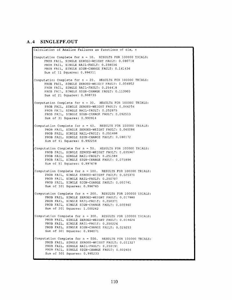
A.4 SINGLEPF.OUT
110
Calculation of Adaline Failures as functions of dim, n
Computation Complete for n = 10. RESULTS FOR 100000 TRIALS:PROB FAIL, SINGLE ZEROED-WEIGHT FAULT: 0.080718PROB FAIL, SINGLE RAIL-FAULT: 0.258036PROB FAIL, SINGLE SIGN-CHANGE FAULT: 0.161436Sum of 11 Squares: 0.996311
Computation Complete for n = 20. RESULTS FOR 100000 TRIALS:PROB FAIL, SINGLE ZEROED-WEIGHT FAULT: 0.056952PROB FAIL, SINGLE RAIL-FAULT: 0.254418PROB FAIL, SINGLE SIGN-CHANGE FAULT: 0.113903Sum of 21 Squares: 0.998735
Computation Complete for n = 30. RESULTS FOR 100000 TRIALS:PROB FAIL, SINGLE ZEROED-WEIGHT FAULT: 0.046256PROB FAIL, SINGLE RAIL-FAULT: 0.252875PROB FAIL, SINGLE SIGN-CHANGE FAULT: 0.092513Sum of 31 Squares: 0.990914
Computation Complete for n = 40. RESULTS FOR 100000 TRIALS:PROB FAIL, SINGLE ZEROED-WEIGHT FAULT: 0.040086PROB FAIL, SINGLE RAIL-FAULT: 0.251698PROB FAIL, SINGLE SIGN-CHANGE FAULT: 0.080172Sum of 41 Squares: 0.992254
Computation Complete for n = 50. RESULTS FOR 100000 TRIALS:PROB FAIL, SINGLE ZEROED-WEIGHT FAULT: 0.035947PROB FAIL, SINGLE RAIL-FAULT: 0.251584PROB FAIL, SINGLE SIGN-CHANGE FAULT: 0.071894Sum of 51 Squares: 0.997678
Computation Complete for n = 100. RESULTS FOR 100000 TRIALS:PROB FAIL, SINGLE ZEROED-WEIGHT FAULT: 0.025370PROB FAIL, SINGLE RAIL-FAULT: 0.250707PROB FAIL, SINGLE SIGN-CHANGE FAULT: 0.050741Sum of 101 Squares: 0.996765
Computation Complete for n = 200. RESULTS FOR 100000 TRIALS:PROB FAIL, SINGLE ZEROED-WEIGHT FAULT: 0.017980PROB FAIL, SINGLE RAIL-FAULT: 0.250371PROB FAIL, SINGLE SIGN-CHANGE FAULT: 0.035960Sum of 201 Squares: 1.000242
Computation Complete for n = 300. RESULTS FOR 100000 TRIALS:PROB FAIL, SINGLE ZEROED-WEIGHT FAULT: 0.014626PROB FAIL, SINGLE RAIL-FAULT: 0.250226PROB FAIL, SINGLE SIGN-CHANGE FAULT: 0.029253Sum of 301 Squares: 0.994071
Computation Complete for n = 500. RESULTS FOR 100000 TRIALS:PROB FAIL, SINGLE ZEROED-WEIGHT FAULT: 0.011327PROB FAIL, SINGLE RAIL-FAULT: 0.250191PROB FAIL, SINGLE SIGN-CHANGE FAULT: 0.022654Sum of 501 Squares: 0.995233

A.5 MULTIPLEPF.OUT
111
Calculation of Adaline Failures as functions of dim, nMultiple Fault Cases
Computation Complete for n = 10. RESULTS FOR 100000 TRIALS:PROB FAIL, MUL. ZEROED-WEIGHT FAULT:
m = 0: 0.000000m = 1: 0.080431m = 5: 0.234702
PROB FAIL, MUL. RAIL-FAULT:m = 0: 0.000000
m = 1: 0.257499
m = 5: 0.422430
PROB FAIL, MUL. SIGN-CHANGE FAULT:m = 0: 0.000000m = 1: 0.160861
m = 5: 0.469404
Computation Complete for n = 20. RESULTS FOR 100000 TRIALS:PROB FAIL, MUL. ZEROED-WEIGHT FAULT:
m = 0: 0.000000
m = 2: 0.089945m = 10: 0.243087
PROB FAIL, MUL. RAIL-FAULT:m = 0: 0.000000
m = 2: 0.317708
m = 10: 0.448419
PROB FAIL, MUL. SIGN-CHANGE FAULT:m = 0: 0.000000
m = 2: 0.179891
m = 10: 0.486174
Computation Complete for n = 30. RESULTS FOR 100000 TRIALS:PROB FAIL, MUL. ZEROED-WEIGHT FAULT:
m = 0: 0.000000
m = 3: 0.093300m = 15: 0.243773
PROB FAIL, MUL. RAIL-FAULT:m = 0: 0.000000
m = 3: 0.346450
m = 15: 0.458082
PROB FAIL, MUL. SIGN-CHANGE FAULT:m = 0: 0.000000
m = 3: 0.186600
m = 15: 0.487545
Computation Complete for n = 40. RESULTS FOR 100000 TRIALS:PROB FAIL, MUL. ZEROED-WEIGHT FAULT:
m = 0: 0.000000
m = 4: 0.095171m = 20: 0.245338
PROB FAIL, MUL. RAIL-FAULT:m = 0: 0.000000
m = 4: 0.364110
m = 20: 0.461909
PROB FAIL, MUL. SIGN-CHANGE FAULT:m = 0: 0.000000
m = 4: 0.190342
m = 20: 0.490676
CONTE

Computation Complete for n = 50. RESULTS FOR 100000 TRIALS:PROB FAIL, MUL. ZEROED-WEIGHT FAULT:
m = 0: 0.000000m = 5: 0.096807m = 25: 0.246685
PROB FAIL, MUL. RAIL-FAULT:m = 0: 0.000000m = 5: 0.377793m = 25: 0.467392
PROB FAIL, MUL. SIGN-CHANGE FAULT:m = 0: 0.000000m = 5: 0.193613m = 25: 0.493371
Computation Complete for n = 100. RESULTS FOR 100000 TRIALS:PROB FAIL, MUL. ZEROED-WEIGHT FAULT:
m = 1: 0.025390m = 10: 0.099310m = 50: 0.247918
PROB FAIL, MUL. RAIL-FAULT:m = 1: 0.250688m = 10: 0.411250m = 50: 0.476614
PROB FAIL, MUL. SIGN-CHANGE FAULT:m = 1: 0.050780m = 10: 0.198621m = 50: 0.495836
Computation Complete for n = 200. RESULTS FOR 100000 TRIALS:PROB FAIL, MUL. ZEROED-WEIGHT FAULT:
m = 2: 0.028232m = 20: 0.100999m = 100: 0.249260
PROB FAIL, MUL. RAIL-FAULT:m = 2: 0.305295m = 20: 0.436569m = 100: 0.483615
PROB FAIL, MUL. SIGN-CHANGE FAULT:m = 2: 0.056463m = 20: 0.201999m = 100: 0.498520
Computation Complete for n = 300. RESULTS FOR 100000 TRIALS:PROB FAIL, MUL. ZEROED-WEIGHT FAULT:
m = 3: 0.029282m = 30: 0.101175m = 150: 0.248367
PROB FAIL, MUL. RAIL-FAULT:m = 3: 0.334698m = 30: 0.447868m = 150: 0.486370
PROB FAIL, MUL. SIGN-CHANGE FAULT:m = 3: 0.058563m = 30: 0.202350m = 150: 0.496733
Computation Complete for n = 500. RESULTS FOR 100000 TRIALS:PROB FAIL, MUL. ZEROED-WEIGHT FAULT:
m = 5: 0.030244m = 50: 0.101575m = 250: 0.248902
PROB FAIL, MUL. RAIL-FAULT:m = 5: 0.367345 CONTE
112

113
m = 50: 0.459844
m = 250: 0.490417
PROB FAIL, MUL. SIGN-CHANGE FAULT:
m = 5: 0.060489
m = 50: 0.203149
m = 250: 0.497804

APPENDIX B: MATHEMATICAL DERIVATIONS
This appendix presents some of the mathematical detail which was not directly relevant
to the principles developed in the body of the text.
B.1 REDUCTION OF GAMMA FUNCTION RATIOS
In §3.4.2, the probability density function for a single weight component, fw(w) is
given by:
fW(w) = 2 (1-w2)(n- 3)/2
Since the variable n is an integer, the fractionI I(2-- n
(3-49), (Bl-1)
can be reduced to a form not
explictly requiring the gamma function. For n even, n is also an integer and the gamma
function can be calculated directly using as 1(x) = (x-l)!, for x an integer. For n even,en-i. 1however, n -y is an odd multiple of - and the gamma function property F(x+ 1)
used in conjunction with F 1 )
= xF(x) must be
= r-. The converse is true for n odd.
The formula for the gamma function of an odd multiple of is2
F(m + = (2m-1)!! I-2-m
where m is an integer and x!! is the semifactorial function
1 x = -1, 0x!! = x*(x-2)*(x-4)*...*5*3 x odd
x*(x-2).(x-4)...*..4.2 x even
given by [49]:
(B1-2)
(B1-3)
The left side of eq. (B 1-2) can be rephrased as
F(m+ =
= (21 + 1) (B 1-4)
Using the property of the gamma function, F(y+ 1) = yF(y), the right side of eq. (B 1-4) is:
114
- +F(m - - + 1)2

F(2 + 1)2 +1
2m- 1 2m-12 ( 2 )2m- 1( 1)
- 2 m -2
Concatenating eqs. (B 1-4) and (B 1-5),
( 1 2m-1m-m _222 2Fm-2 2 F(m=+ 12)
\ 2/ 2m-1 2
and from eq. (B2-2)
r(m_ (2m-1)!! En)2 2m-1 ( 2m
F(m- =2 (2m-1)!!42 2m-1 * 2m
F(m- )= (2m-3)!! 4-2 2m-1
So, for n even, n = 2m, (m an integer)
F(2) = - 1 _ ) ! = (
and F( ) = (m - = (n-3)!! --2 2(n-2)/2
And, for n odd, n = 2m+1, m = n 1 (m an integer)
(2 = 7(m + )= (n-2)!! H-2-(n-1)/2
and -( = F(m) = (m-)! = (
Using eqs. (B 1-7) and eqs. (B 1-8), the ratio ( n ) becomesUsing eqs. (B 1-7) and eqs. (B 1-8), the ratio 2 becomes
F@ Yr(n-1 2 [-
( ) 2(n-2)/2
(n-2)!!
2(n-1)/2(n-32*
n even
n odd
For obvious notational convenience, the left side of eq. (B 1-9) is used in the text.
115
(B 1-5)
(B 1-6)
(B 1-7a)
(B 1-7b)
(B1-8a)
(B1-8b)
(B 1-9)

B.2 VARIANCE OF SINGLE COMPONENT PROBABILITY DENSITY FUNCTION
This section derives the variance of a single component of an n-dimensional unit vector.
That variable, w, has a probability density function given by
f(w) = -w2)(n-3)/2 (3-49), (B2-1)
By definition, the variance is the second central moment
a2 (w) = E { (w - E w }) 2 } (B2-2)
but fw(w) is an even function, so E { w } = 0, and
y2 (w) = E { w2 } (B2-3)
The expected value can be found through integration. The range of integration is given by the
range of the value of w, w e [-1, +1].
1
E =w2 2) w42(1-w2)( n-3)/2 dw (B2-4)
-1
-= (W2(l1-w2)(n-3)/2)dw (B2-5)
and since both w2 and (l-w2)(n 3)/2 are even functions, their product is even and the integral
can be reduced to1
E w2 }= \ 2 2 J(w2(1-w2)(n-3)/2)dw (B2-6)
From here, integrals tables are used. From Dwight [15], entry 855.41,
1 F(p+1)F(m_)fxm(1 - x2)Pdx = (B2-7)0 2F p+m 3
So with m = 2 and p - n-3
116
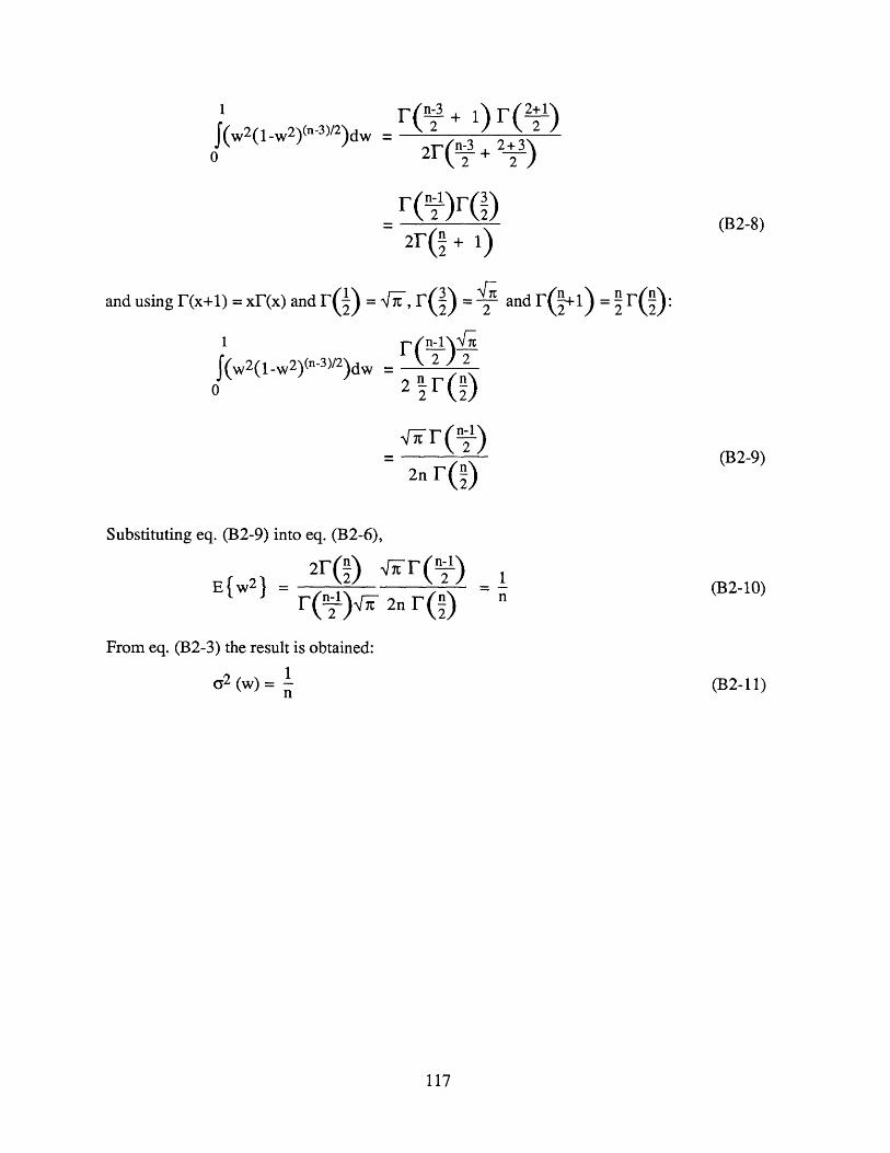
2Fn-3 + q+3)2( 2 2)
and using F(x+1) = xF(x) and F() =
J(w2(1_w2)(n-3)/2)dw0
21F (+ 1
•-, T( =•(2)=2 2
2n(2n( )
(B2-8)
and (• +I)= n ():
(B2-9)
Substituting eq. (B2-9) into eq. (B2-6),
E2 w2( ) 4-- f (n2-1)F 2n - 2)
From eq. (B2-3) the result is obtained:
(2 (w) = 1n
1
J(w2(1-w2)(n-3)/2)dw
1n (B2-10)
(B2-11)
117
][(+n-3 + -(2+12 2)

B.3 CLOSED-FORM SOLUTION FOR THE ADALINE FAILURE PROBABILITY
FOR THE SINGLE ZEROED-WEIGHT FAULT
In §3.5, the probability of adaline failure for the single zeroed-weight fault is given by
2F n+1 1P0(n) = sin-1(w)(1-w2)(n-2)/2dw
F(n) n t3/ 2 0(3-66), (B3-1)
The integral can be solved by creating a new variable 0, such that
w = sine, or 0 = sin- 1(w)
so that dw = cosO dO
and since (sin-) 2 + (cosw)2 = 1,
cosO = (1 - w2)1/2
1 /1)
dw = (1
- w2
dO
(B3-3)
(B3-4)
Setting the constant term in (B3-1) to Cn
2F(n~)Cn =
2 3/2
and substituting eqs. (B3-2) through (B3-5) into eq. (B3-1),
C c/2PF(n) = Cn f0(cos0)n-3d0
(B3-5)
(B3-6)
From here, tables of definite integrals can be used. Entry 2 on p. 386 of Prudnikow et al [37]
states for k > 0:
[k-12
(B3-2)
fx(cosx)kdx0
where
(1-k+2 k - A (k-1)!!t -- ~J~2] 4k!! -
j=0
x!! is the semifactorial function defined in eq. (B 1-3)
(x) =x. (x+1) ... * (x +j- 1)
118
(B3-7)

[x] is the largest integer up to and including x
1, k evenA= 2 k odd
So, for k odd,
[k+] =k+1 and [k-1] = k-1
2 ~2 2 2
and for k even,
[k+] = and k-1 k-2=•and
-22 2 2 2Eq. (B3-7) can be used to solve eq. (B3-6) for n > 3. The result is
For n odd, n > 3:
(n-5)2
j=0
2-2)(3PF(n) = (2 )
Fn ]F I73/2 3 (5)((2j +21- n)(n
and
For n even, n > 3:
PF(n F()232AFn) = r- r/
2 )32
(n-4)
j=2
j=0
2 2 -) (3 - ) ... (J+
(3 ) )...( 2j +21 - n)( n 3 - 2j) 2
Eqs. (B3-8) support the conclusion that a closed-form solution is not necessarily the
best presentation for PF. Computer-aided solutions, even if approximations, are much more
informative.
119
+1(B3-8a)
(B3-8b)
- )
-3 -2j )2
-0 ... (
7t(n-4)!!I2(n-3)!!