e charge and electric field - · pdf file21/04/2013 · if you carry a net charge,...
TRANSCRIPT

21-1
ELECTRIC CHARGE AND ELECTRIC FIELD
21.1. (a) IDENTIFY and SET UP: Use the charge of one electron 19( 1.602 10 C)−− × to find the number of electrons required to produce the net charge. EXECUTE: The number of excess electrons needed to produce net charge q is
910
19
3.20 10 C 2.00 10 electrons.1.602 10 C/electron
qe
−
−
− ×= = ×
− − ×
(b) IDENTIFY and SET UP: Use the atomic mass of lead to find the number of lead atoms in 38.00 10 kg−× of lead. From this and the total number of excess electrons, find the number of excess electrons per lead atom. EXECUTE: The atomic mass of lead is 3207 10 kg/mol,−× so the number of moles in 38.00 10 kg−× is
3tot
3
8.00 10 kg 0.03865 mol.207 10 kg/mol
mnM
−
−
×= = =
× AN (Avogadro’s number) is the number of atoms in 1 mole, so the
number of lead atoms is 23 22A (0.03865 mol)(6.022 10 atoms/mol) = 2.328 10 atoms.N nN= = × × The number of
excess electrons per lead atom is 10
1322
2.00 10 electrons 8.59 10 .2.328 10 atoms
−×= ×
×
EVALUATE: Even this small net charge corresponds to a large number of excess electrons. But the number of atoms in the sphere is much larger still, so the number of excess electrons per lead atom is very small.
21.2. IDENTIFY: The charge that flows is the rate of charge flow times the duration of the time interval. SET UP: The charge of one electron has magnitude 191.60 10 C.e −= × EXECUTE: The rate of charge flow is 20,000 C/s and 4100 s 1.00 10 s.t μ −= = ×
4(20,000 C/s)(1.00 10 s) 2.00 C.Q −= × = The number of electrons is 19e 19 1.25 10 .
1.60 10 CQn −= = ××
EVALUATE: This is a very large amount of charge and a large number of electrons. 21.3. IDENTIFY: From your mass estimate the number of protons in your body. You have an equal number of electrons.
SET UP: Assume a body mass of 70 kg. The charge of one electron is 191.60 10 C.−− × EXECUTE: The mass is primarily protons and neutrons of 271.67 10 kg.m −= × The total number of protons and
neutrons is 28p and n 27
70 kg 4.2 10 .1.67 10 kg
n −= = ××
About one-half are protons, so 28p e2.1 10n n= × = . The number of
electrons is about 282.1 10 .× The total charge of these electrons is 19 28 9( 1.60 10 C/electron)(2.10 10 electrons) 3.35 10 C.Q −= − × × = − ×
EVALUATE: This is a huge amount of negative charge. But your body contains an equal number of protons and your net charge is zero. If you carry a net charge, the number of excess or missing electrons is a very small fraction of the total number of electrons in your body.
21.4. IDENTIFY: Use the mass m of the ring and the atomic mass M of gold to calculate the number of gold atoms. Each atom has 79 protons and an equal number of electrons. SET UP: 23
A 6.02 10 atoms/molN = × . A proton has charge +e. EXECUTE: The mass of gold is 17.7 g and the atomic weight of gold is 197 g mol. So the number of atoms
is 23 22A
17.7 g(6.02 10 atoms/mol) 5.41 10 atoms197 g molN n ⎛ ⎞= × = ×⎜ ⎟⎝ ⎠
. The number of protons is
22 24p (79 protons/atom)(5.41 10 atoms) 4.27 10 protonsn = × = × . 19 5
p( )(1.60 10 C/proton) 6.83 10 CQ n −= × = × .
(b) The number of electrons is 24e p 4.27 10 .n n= = ×
EVALUATE: The total amount of positive charge in the ring is very large, but there is an equal amount of negative charge.
21

21-2 Chapter 21
21.5. IDENTIFY: Apply 1 22
k q qF
r= and solve for r.
SET UP: 650 NF = .
EXECUTE: 9 2 2 2
1 2 3(8.99 10 N m /C )(1.0 C) 3.7 10 m 3.7 km650 N
k q qr
F× ⋅
= = = × =
EVALUATE: Charged objects typically have net charges much less than 1 C. 21.6. IDENTIFY: Apply Coulomb's law and calculate the net charge q on each sphere.
SET UP: The magnitude of the charge of an electron is 191.60 10 Ce −= × .
EXECUTE: 2
20
1 .4
qFrπ
=P
This gives 2 21 2 160 04 4 (4.57 10 N)(0.200 m) 1.43 10 C.q Frπ π − −= = × = ×P P And
therefore, the total number of electrons required is 16 19/ (1.43 10 C)/(1.60 10 C/electron) 890 electrons.n q e − −= = × × =
EVALUATE: Each sphere has 890 excess electrons and each sphere has a net negative charge. The two like charges repel.
21.7. IDENTIFY: Apply Coulomb’s law. SET UP: Consider the force on one of the spheres. (a) EXECUTE: 1 2q q q= =
21 2
2 20 0
14 4
q q qFr rπ π
= =P P
so 79 2 2
0
0.220 N0.150 m 7.42 10 C (on each)(1/4 ) 8.988 10 N m /C
Fq rπ
−= = = ×× ⋅P
(b) 2 14q q= 2
1 2 12 2
0 0
1 44 4
q q qFr rπ π
= =P P
so 7 71 11 2 2
0 0
(7.42 10 C) = 3.71 10 C.4(1/4 ) (1/4 )
F Fq r rπ π
− −= = = × ×P P
And then 62 14 1.48 10 C.q q −= = ×
EVALUATE: The force on one sphere is the same magnitude as the force on the other sphere, whether the sphere have equal charges or not.
21.8. IDENTIFY: Use the mass of a sphere and the atomic mass of aluminum to find the number of aluminum atoms in one sphere. Each atom has 13 electrons. Apply Coulomb's law and calculate the magnitude of charge q on each sphere. SET UP: 23
A 6.02 10 atoms/molN = × . eq n e′= , where en′ is the number of electrons removed from one sphere and added to the other. EXECUTE: (a) The total number of electrons on each sphere equals the number of protons.
24e p A
0.0250 kg(13)( ) 7.25 10 electrons0.026982 kg mol
n n N⎛ ⎞
= = = ×⎜ ⎟⎝ ⎠
.
(b) For a force of 41.00 10× N to act between the spheres, 2
42
0
11.00 10 N4
qFrπ
= × =P
. This gives
4 2 404 (1.00 10 N)(0.0800 m) 8.43 10 Cq π −= × = ×P . The number of electrons removed from one sphere and
added to the other is 15e / 5.27 10 electrons.n q e′ = = ×
(c) 10e e/ 7.27 10n n −′ = × .
EVALUATE: When ordinary objects receive a net charge the fractional change in the total number of electrons in the object is very small .
21.9. IDENTIFY: Apply F ma= , with 1 22
q qF k
r= .
SET UP: 225.0 245 m/sa g= = . An electron has charge 191.60 10 C.e −− = − ×
EXECUTE: 3 2(8.55 10 kg)(245 m/s ) 2.09 NF ma −= = × = . The spheres have equal charges q, so 2
2
qF kr
= and
69 2 2
2.09 N(0.150 m) 2.29 10 C8.99 10 N m /C
Fq rk
−= = = ×× ⋅
. 6
1319
2.29 10 C 1.43 10 electrons1.60 10 C
qN
e
−
−
×= = = ×
×. The
charges on the spheres have the same sign so the electrical force is repulsive and the spheres accelerate away from each other.

Electric Charge and Electric Field 21-3
EVALUATE: As the spheres move apart the repulsive force they exert on each other decreases and their acceleration decreases.
21.10. (a) IDENTIFY: The electrical attraction of the proton gives the electron an acceleration equal to the acceleration due to gravity on earth. SET UP: Coulomb’s law gives the force and Newton’s second law gives the acceleration this force produces.
1 22
0
14
q qma
rπ=
P and
2
0
4
ermaπ
=P
.
EXECUTE: r =( )( )
( )( )
29 2 2 19
31 2
9.00 10 N m /C 1.60 10 C
9.11 10 kg 9.80 m/s
−
−
× ⋅ ×
× = 5.08 m
EVALUATE: The electron needs to be about 5 m from a single proton to have the same acceleration as it receives from the gravity of the entire earth. (b) IDENTIFY: The force on the electron comes from the electrical attraction of all the protons in the earth. SET UP: First find the number n of protons in the earth, and then find the acceleration of the electron using Newton’s second law, as in part (a).
n = mE/mp = (5.97 × 1024 kg)/(1.67 × 2710− kg) = 3.57 × 1051 protons.
a = F/m =
p e 22
0 E 02
e e E
1 14 4
q qne
Rm m R
π π=
P P .
EXECUTE: a = (9.00 × 10⁹ N ⋅ m2/C2)(3.57 × 1051)(1.60 × 1910− C)2/[(9.11 × 3110− kg)(6.38 × 10⁶ m)2] = 2.22 × 1040 m/s2. One can ignore the gravitation force since it produces an acceleration of only 9.8 m/s2 and hence is much much less than the electrical force. EVALUATE: With the electrical force, the acceleration of the electron would nearly 1040 times greater than with gravity, which shows how strong the electrical force is.
21.11. IDENTIFY: In a space satellite, the only force accelerating the free proton is the electrical repulsion of the other proton. SET UP: Coulomb’s law gives the force, and Newton’s second law gives the acceleration: a = F/m =
0(1/ 4 )πP (e2/r2)/m. EXECUTE: (a) a = (9.00 × 10⁹ N ⋅ m2/C2)(1.60 × 10-19 C)2/[(0.00250 m)2(1.67 × 10⁻²⁷ kg)] = 2.21 × 10⁴ m/s2. (b) The graphs are sketched in Figure 21.11. EVALUATE: The electrical force of a single stationary proton gives the moving proton an initial acceleration about 20,000 times as great as the acceleration caused by the gravity of the entire earth. As the protons move farther apart, the electrical force gets weaker, so the acceleration decreases. Since the protons continue to repel, the velocity keeps increasing, but at a decreasing rate.
Figure 21.11
21.12. IDENTIFY: Apply Coulomb’s law. SET UP: Like charges repel and unlike charges attract.
EXECUTE: (a) 1 22
0
14
q qF
rπ=
P. This gives
62
20
(0.550 10 C)10.200 N4 (0.30 m)
qπ
−×=
P and 6
2 3.64 10 Cq −= + × . The
force is attractive and 1 0q < , so 62 3.64 10 Cq −= + × .
(b) 0.200F = N. The force is attractive, so is downward. EVALUATE: The forces between the two charges obey Newton's third law.

21-4 Chapter 21
21.13. IDENTIFY: Apply Coulomb’s law. The two forces on 3q must have equal magnitudes and opposite directions. SET UP: Like charges repel and unlike charges attract.
EXECUTE: The force 2F that 2q exerts on 3q has magnitude 2 32 2
2
q qF k
r= and is in the +x direction. 1F must be in
the x− direction, so 1q must be positive. 1 2F F= gives 1 3 2 32 2
1 2
q q q qk k
r r= .
2 21
1 22
2.00 cm(3.00 nC) 0.750 nC4.00 cm
rq qr
⎛ ⎞ ⎛ ⎞= = =⎜ ⎟ ⎜ ⎟⎝ ⎠⎝ ⎠
.
EVALUATE: The result for the magnitude of 1q doesn’t depend on the magnitude of 2q . 21.14. IDENTIFY: Apply Coulomb’s law and find the vector sum of the two forces on Q.
SET UP: The force that 1q exerts on Q is repulsive, as in Example 21.4, but now the force that 2q exerts is attractive. EXECUTE: The x-components cancel. We only need the y-components, and each charge contributes equally.
6 6
1 2 20
1 (2.0 10 C) (4.0 10 C) sin 0.173 N (since sin 0.600).4 (0.500 m)y yF F α απ
− −× ×= = − = − =
P Therefore, the total force is
2 0.35 N,F = in the -directiony− . EVALUATE: If 1q is 2.0 Cμ− and 2q is 2.0 Cμ+ , then the net force is in the +y-direction.
21.15. IDENTIFY: Apply Coulomb’s law and find the vector sum of the two forces on 1q .
SET UP: Like charges repel and unlike charges attract, so 2F and 3F are both in the +x-direction.
EXECUTE: 1 2 1 35 42 32 2
12 13
6.749 10 N, 1.124 10 Nq q q q
F k F kr r
− −= = × = = × . 42 3 1.8 10 NF F F −= + = × .
41.8 10 NF −= × and is in the +x-direction. EVALUATE: Comparing our results to those in Example 21.3, we see that 1 on 3 3 on 1= −F F , as required by Newton’s third law.
21.16. IDENTIFY: Apply Coulomb’s law and find the vector sum of the two forces on 2q .
SET UP: 2 on 1F is in the +y-direction.
EXECUTE: ( )
9 2 2 6 6
2on 1 2
(9.0 10 N m C ) (2.0 10 C) (2.0 10 C) 0.100 N0.60 m
F− −× ⋅ × ×
= = . ( )2 on 1 0x
F = and
( )2 on 1 0.100 Ny
F = + . on 1QF is equal and opposite to 1 on QF (Example 21.4), so ( ) on 1 0.23NQ xF = − and
( ) on 1 0.17 NQ yF = . ( ) ( )2 on 1 on 1 0.23 Nx Qx x
F F F= + = − . ( ) ( )2 on 1 on 1 0.100 N 0.17 N 0.27 Ny Qy yF F F= + = + = .
The magnitude of the total force is ( ) ( )2 20.23 N 0.27 N 0.35 N.F = + = 1 0.23tan 400.27
− = ° , so F is
40° counterclockwise from the +y axis, or 130° counterclockwise from the +x axis. EVALUATE: Both forces on 1q are repulsive and are directed away from the charges that exert them.
21.17. IDENTIFY and SET UP: Apply Coulomb’s law to calculate the force exerted by 2q and 3q on 1.q Add these forces as vectors to get the net force. The target variable is the x-coordinate of 3.q
EXECUTE: 2F is in the x-direction.
1 22 22
12
3.37 N, so 3.37 Nx
q qF k F
r= = = +
2 3 and 7.00 Nx x x xF F F F= + = −
3 2 7.00 N 3.37 N 10.37 Nx x xF F F= − = − − = − For 3xF to be negative, 3q must be on the x− -axis.
1 3 1 33 2
3
, so 0.144 m, so 0.144 mq q k q q
F k x xx F
= = = = −
EVALUATE: 2q attracts 1q in the x+ -direction so 3q must attract 1q in the x− -direction, and 3q is at negative x.

Electric Charge and Electric Field 21-5
21.18. IDENTIFY: Apply Coulomb’s law. SET UP: Like charges repel and unlike charges attract. Let 21F be the force that 2q exerts on 1q and let 31F be the force that 3q exerts on 1q . EXECUTE: The charge 3q must be to the right of the origin; otherwise both 2 3andq q would exert forces in the
x+ direction. Calculating the two forces: 9 2 2 6 6
1 221 2 2
0 12
1 (9 10 N m C )(3.00 10 C)(5.00 10 C) 3.375 N4 (0.200 m)
q qF
rπ
− −× ⋅ × ×= = =
P, in the +x direction.
9 2 2 6 6 2
31 2 213 13
(9 10 N m C ) (3.00 10 C) (8.00 10 C) 0.216 N mFr r
− −× ⋅ × × ⋅= = , in the x− direction.
We need 21 31 7.00 NxF F F= − = − , so 2
213
0.216 N m3.375 N 7.00 Nr
⋅− = − .
2
130.216 N m 0.144 m
3.375 N 7.00 Nr ⋅
= =+
. 3q
is at 0.144 mx = . EVALUATE: 31 10.4 N.F = 31F is larger than 21,F because 3q is larger than 2q and also because 13r is less than 12.r
21.19. IDENTIFY: Apply Coulomb’s law to calculate the force each of the two charges exerts on the third charge. Add these forces as vectors. SET UP: The three charges are placed as shown in Figure 21.19a.
Figure 21.19a
EXECUTE: Like charges repel and unlike attract, so the free-body diagram for 3q is as shown in Figure 21.19b.
1 31 2
0 13
14
q qF
rπ=
P
2 32 2
0 23
14
q qF
rπ=
P
Figure 21.19b 9 9
9 2 2 61 2
(1.50 10 C)(5.00 10 C)(8.988 10 N m /C ) 1.685 10 N(0.200 m)
F− −
−× ×= × ⋅ = ×
9 99 2 2 7
2 2
(3.20 10 C)(5.00 10 C)(8.988 10 N m /C ) 8.988 10 N(0.400 m)
F− −
−× ×= × ⋅ = ×
The resultant force is 1 2.R F F= + 0.xR =
6 7 61 2 1.685 10 N +8.988 10 N = 2.58 10 N.yR F F − − −= + = × × ×
The resultant force has magnitude 62.58 10 N −× and is in the –y-direction. EVALUATE: The force between 1 3 and q q is attractive and the force between 2 3and q q is replusive.
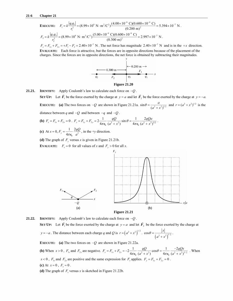
21.20. IDENTIFY: Apply 2
qqF k
r′
= to each pair of charges. The net force is the vector sum of the forces due to 1q and 2.q
SET UP: Like charges repel and unlike charges attract. The charges and their forces on 3q are shown in Figure 21.20.
21-6 Chapter 21
EXECUTE: 9 9
1 3 9 2 2 71 2 2
1
(4.00 10 C)(0.600 10 C)(8.99 10 N m /C ) 5.394 10 N(0.200 m)
q qF k
r
− −−× ×
= = × ⋅ = × .
9 92 3 9 2 2 7
2 2 22
(5.00 10 C)(0.600 10 C)(8.99 10 N m /C ) 2.997 10 N(0.300 m)
q qF k
r
− −−× ×
= = × ⋅ = × .
71 2 1 2 2.40 10 Nx x xF F F F F −= + = + − = × . The net force has magnitude 72.40 10 N−× and is in the x+ direction.
EVALUATE: Each force is attractive, but the forces are in opposite directions because of the placement of the charges. Since the forces are in opposite directions, the net force is obtained by subtracting their magnitudes.
Figure 21.20
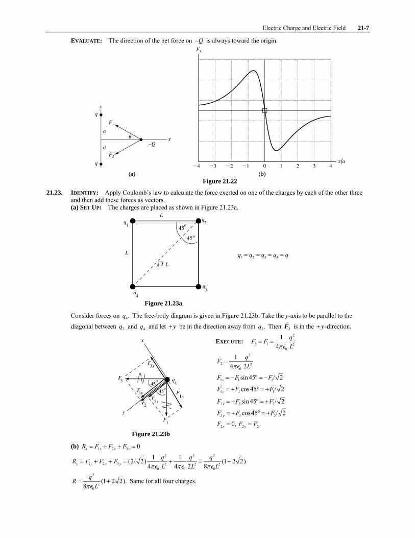
21.21. IDENTIFY: Apply Coulomb’s law to calculate each force on Q− .
SET UP: Let 1F be the force exerted by the charge at y a= and let 2F be the force exerted by the charge at .y a= −
EXECUTE: (a) The two forces on Q− are shown in Figure 21.21a. 2 2 1/ 2sin( )
aa x
θ =+
and 2 2 1/ 2( )r a x= + is the
distance between q and Q− and between q− and Q− .
(b) 1 2 0x x xF F F= + = . 1 2 2 2 2 2 3 20 0
1 1 22 sin4 ( ) 4 ( )y y y
qQ qQaF F Fa x a x
θπ π
= + = =+ +P P
.
(c) 20
1 2At 0,4y
qQx Faπ
= =P
, in the +y direction.
(d) The graph of yF versus x is given in Figure 21.21b.
EVALUATE: 0xF = for all values of x and 0yF > for all x.
Figure 21.21
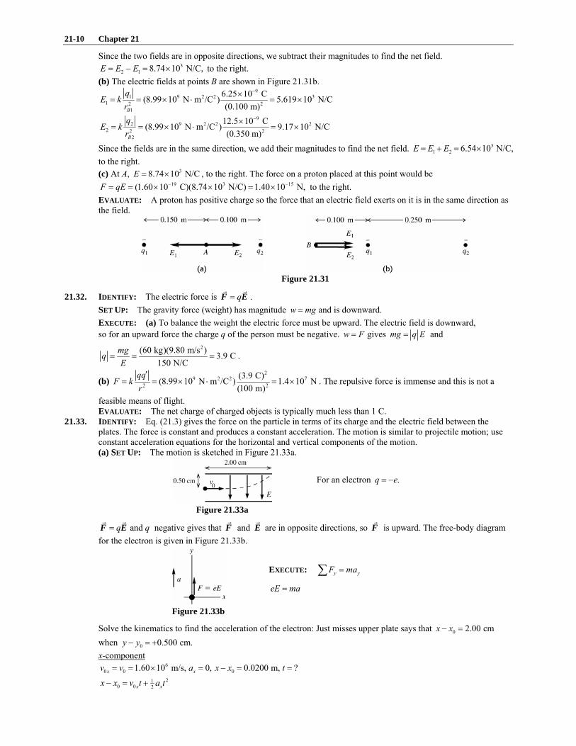
21.22. IDENTIFY: Apply Coulomb’s law to calculate each force on Q− .
SET UP: Let 1F be the force exerted by the charge at y a= and let 2F be the force exerted by the charge at
y a= − . The distance between each charge q and Q is ( )1/ 22 2r a x= + . ( )1/ 22 2
cosx
a xθ =
+.
EXECUTE: (a) The two forces on Q− are shown in Figure 21.22a.
(b) When 0x > , 1xF and 2xF are negative. 1 2 2 2 2 2 3 / 20 0
1 1 22 cos4 ( ) 4 ( )x x x
qQ qQxF F Fa x a x
θπ π
−= + = − =
+ +P P. When
0x < , 1xF and 2xF are positive and the same expression for xF applies. 1 2 0y y yF F F= + = .
(c) At 0x = , 0xF = . (d) The graph of xF versus x is sketched in Figure 21.22b.
Electric Charge and Electric Field 21-7
EVALUATE: The direction of the net force on Q− is always toward the origin.
Figure 21.22
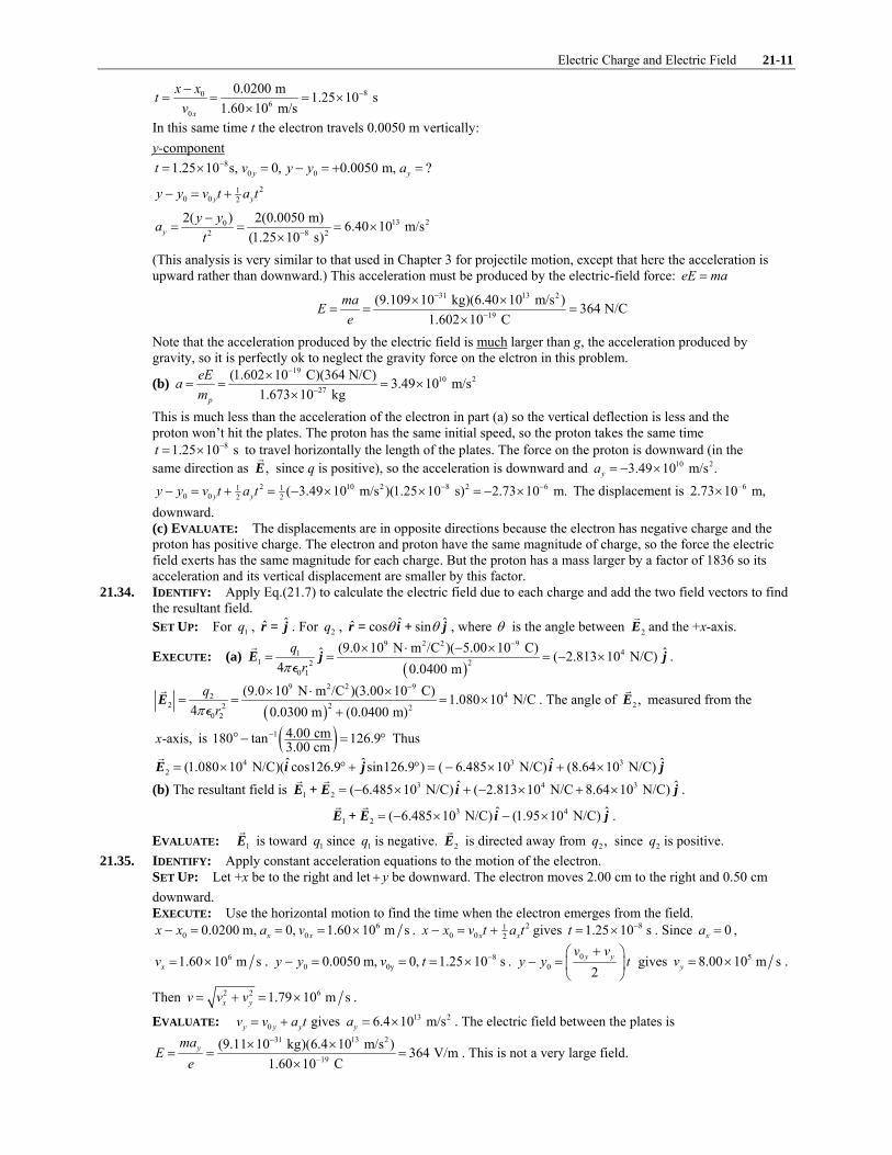
21.23. IDENTIFY: Apply Coulomb’s law to calculate the force exerted on one of the charges by each of the other three and then add these forces as vectors. (a) SET UP: The charges are placed as shown in Figure 21.23a.
1 2 3 4q q q q q= = = =
Figure 21.23a Consider forces on 4.q The free-body diagram is given in Figure 21.23b. Take the y-axis to be parallel to the
diagonal between 2q and 4q and let y+ be in the direction away from 2.q Then 2F is in the y+ -direction.
EXECUTE: 2
3 1 20
14
qF FLπ
= =P
2
2 20
14 2
qFLπ
=P
1 1 1sin 45 / 2xF F F= − ° = −
1 1 1cos45 / 2yF F F= + ° = +
3 3 3sin 45 / 2xF F F= + ° = +
3 3 3cos45 / 2yF F F= + ° = +
2 2 20, x yF F F= = Figure 21.23b
(b) 1 2 3 0x x x xR F F F= + + = 2 2 2
1 2 3 2 2 20 0 0
1 1(2/ 2) (1 2 2)4 4 2 8y y y y
q q qR F F FL L Lπ π π
= + + = + = +P P P
2
20
(1 2 2).8
qRLπ
= +P
Same for all four charges.

21-8 Chapter 21
EVALUATE: In general the resultant force on one of the charges is directed away from the opposite corner. The forces are all repulsive since the charges are all the same. By symmetry the net force on one charge can have no component perpendicular to the diagonal of the square.
21.24. IDENTIFY: Apply 2
k qqF
r′
= to find the force of each charge on q+ . The net force is the vector sum of the
individual forces. SET UP: Let 1 2.50 Cq μ= + and 2 3.50 Cq μ= − . The charge q+ must be to the left of 1q or to the right of 2q in order for the two forces to be in opposite directions. But for the two forces to have equal magnitudes, q+ must be closer to the charge 1q , since this charge has the smaller magnitude. Therefore, the two forces can combine to give zero net force only in the region to the left of 1q . Let q+ be a distance d to the left of 1q , so it is a distance
0.600 md + from 2q .
EXECUTE: 1 2F F= gives 1 22 2( 0.600 m)
kq q kq qd d
=+
. 1
2
( 0.600 m) (0.8452)( 0.600 m)q
d d dq
= ± + = ± + . d must
be positive, so (0.8452)(0.600 m) 3.27 m1 0.8452
d = =−
. The net force would be zero when q+ is at 3.27 mx = − .
EVALUATE: When q+ is at 3.27 mx = − , 1F is in the x− direction and 2F is in the +x direction. 21.25. IDENTIFY: F q E= . Since the field is uniform, the force and acceleration are constant and we can use a constant
acceleration equation to find the final speed. SET UP: A proton has charge +e and mass 271.67 10 kg−× .
EXECUTE: (a) 19 3 16(1.60 10 C)(2.75 10 N/C) 4.40 10 NF − −= × × = ×
(b) 16
11 227
4.40 10 N 2.63 10 m/s1.67 10 kg
Fam
−
−
×= = = ×
×
(c) 0x x xv v a t= + gives 11 2 6 5(2.63 10 m/s )(1.00 10 s) 2.63 10 m/sv −= × × = × EVALUATE: The acceleration is very large and the gravity force on the proton can be ignored.
21.26. IDENTIFY: For a point charge, 2
qE k
r= .
SET UP: E is toward a negative charge and away from a positive charge. EXECUTE: (a) The field is toward the negative charge so is downward.
99 2 2
2
3.00 10 C(8.99 10 N m /C ) 432 N/C(0.250 m)
E−×
= × ⋅ = .
(b) 9 2 2 9(8.99 10 N m /C )(3.00 10 C) 1.50 m
12.0 N/Ck q
rE
−× ⋅ ×= = =
EVALUATE: At different points the electric field has different directions, but it is always directed toward the negative point charge.
21.27. IDENTIFY: The acceleration that stops the charge is produced by the force that the electric field exerts on it. Since the field and the acceleration are constant, we can use the standard kinematics formulas to find acceleration and time. (a) SET UP: First use kinematics to find the proton’s acceleration. 0xv = when it stops. Then find the electric field needed to cause this acceleration using the fact that F = qE. EXECUTE: 2 2
0 02 ( )x x xv v a x x= + − . 0 = (4.50 × 10⁶ m/s)2 + 2a(0.0320 m) and a = 3.16 × 10¹⁴ m/s2. Now find the
electric field, with q = e. eE = ma and E = ma/e = (1.67 × 2710− kg)(3.16 × 10¹⁴ m/s2)/(1.60 × 1910− C) = 3.30 × 10⁶ N/C, to the left. (b) SET UP: Kinematics gives v = v0 + at, and v = 0 when the electron stops, so t = v0/a. EXECUTE: t = v0/a = (4.50 × 10⁶ m/s)/(3.16 × 1014 m/s2) = 1.42 × 810− s = 14.2 ns (c) SET UP: In part (a) we saw that the electric field is proportional to m, so we can use the ratio of the electric fields. e p e p/ /E E m m= and ( )e e p p/E m m E= .
EXECUTE: Ee = [(9.11 × 3110− kg)/(1.67 × 2710− kg)](3.30 × 106 N/C) = 1.80 × 10³ N/C, to the right EVALUATE: Even a modest electric field, such as the ones in this situation, can produce enormous accelerations for electrons and protons.

Electric Charge and Electric Field 21-9
21.28. IDENTIFY: Use constant acceleration equations to calculate the upward acceleration a and then apply q=F E to calculate the electric field. SET UP: Let +y be upward. An electron has charge q e= − .
EXECUTE: (a) 0 0yv = and ya a= , so 210 0 2y yy y v t a t− = + gives 21
0 2y y at− = . Then
21202 6 2
2( ) 2(4.50 m) 1.00 10 m s(3.00 10 s)
y yat −
−= = = ×
×.
231 12
19
(9.11 10 kg) (1.00 10 m s ) 5.69 N C1.60 10 C
F maEq q
−
−
× ×= = = =
×
The force is up, so the electric field must be downward since the electron has negative charge. (b) The electron’s acceleration is ~ 1110 g , so gravity must be negligibly small compared to the electrical force. EVALUATE: Since the electric field is uniform, the force it exerts is constant and the electron moves with constant acceleration.
21.29. (a) IDENTIFY: Eq. (21.4) relates the electric field, charge of the particle, and the force on the particle. If the particle is to remain stationary the net force on it must be zero. SET UP: The free-body diagram for the particle is sketched in Figure 21.29. The weight is mg, downward. For the net force to be zero the force exerted by the electric field must be upward. The electric field is downward. Since the electric field and the electric force are in opposite directions the charge of the particle is negative.
mg q E=
Figure 21.29
EXECUTE: 3 2
5(1.45 10 kg)(9.80 m/s ) 2.19 10 C and 21.9 C650 N/C
mgq qE
μ−
−×= = = × = −
(b) SET UP: The electrical force has magnitude .EF q E eE= = The weight of a proton is .w mg= EF w= so eE mg=
EXECUTE: 27 2
719
(1.673 10 kg)(9.80 m/s ) 1.02 10 N/C.1.602 10 C
mgEe
−−
−
×= = = ×
×
This is a very small electric field. EVALUATE: In both cases and ( / ) .q E mg E m q g= = In part (b) the /m q ratio is much smaller 8( 10 )−∼ than
in part (a) 2( 10 )−∼ so E is much smaller in (b). For subatomic particles gravity can usually be ignored compared to electric forces.
21.30. IDENTIFY: Apply 20
14
qE
rπ=
P.
SET UP: The iron nucleus has charge 26 .e+ A proton has charge e+ .
EXECUTE: (a) 19
1110 2
0
1 (26)(1.60 10 C) 1.04 10 N/C.4 (6.00 10 m)
Eπ
−
−
×= = ×
×P
(b) 19
11proton 11 2
0
1 (1.60 10 C) 5.15 10 N/C.4 (5.29 10 m)
Eπ
−
−
×= = ×
×P
EVALUATE: These electric fields are very large. In each case the charge is positive and the electric fields are directed away from the nucleus or proton.
21.31. IDENTIFY: For a point charge, 2 .q
E kr
= The net field is the vector sum of the fields produced by each charge. A
charge q in an electric field E experiences a force .q=F E SET UP: The electric field of a negative charge is directed toward the charge. Point A is 0.100 m from q2 and 0.150 m from q1. Point B is 0.100 m from q1 and 0.350 m from q2. EXECUTE: (a) The electric fields due to the charges at point A are shown in Figure 21.31a.
91 9 2 2 3
1 2 21
6.25 10 C(8.99 10 N m /C ) 2.50 10 N/C(0.150 m)A
qE k
r
−×= = × ⋅ = ×
92 9 2 2 4
2 2 22
12.5 10 C(8.99 10 N m /C ) 1.124 10 N/C(0.100 m)A
qE k
r
−×= = × ⋅ = ×
21-10 Chapter 21
Since the two fields are in opposite directions, we subtract their magnitudes to find the net field. 3
2 1 8.74 10 N/C,E E E= − = × to the right. (b) The electric fields at points B are shown in Figure 21.31b.
91 9 2 2 3
1 2 21
6.25 10 C(8.99 10 N m /C ) 5.619 10 N/C(0.100 m)B
qE k
r
−×= = × ⋅ = ×
92 9 2 2 2
2 2 22
12.5 10 C(8.99 10 N m /C ) 9.17 10 N/C(0.350 m)B
qE k
r
−×= = × ⋅ = ×
Since the fields are in the same direction, we add their magnitudes to find the net field. 31 2 6.54 10 N/C,E E E= + = ×
to the right. (c) At A, 38.74 10 N/CE = × , to the right. The force on a proton placed at this point would be
19 3 15(1.60 10 C)(8.74 10 N/C) 1.40 10 N,F qE − −= = × × = × to the right. EVALUATE: A proton has positive charge so the force that an electric field exerts on it is in the same direction as the field.
Figure 21.31
21.32. IDENTIFY: The electric force is q=F E . SET UP: The gravity force (weight) has magnitude w mg= and is downward. EXECUTE: (a) To balance the weight the electric force must be upward. The electric field is downward, so for an upward force the charge q of the person must be negative. w F= gives mg q E= and
2(60 kg)(9.80 m/s ) 3.9 C150 N/C
mgqE
= = = .
(b) 2
9 2 2 72 2
(3.9 C)(8.99 10 N m /C ) 1.4 10 N(100 m)
qqF k
r′
= = × ⋅ = × . The repulsive force is immense and this is not a
feasible means of flight. EVALUATE: The net charge of charged objects is typically much less than 1 C.
21.33. IDENTIFY: Eq. (21.3) gives the force on the particle in terms of its charge and the electric field between the plates. The force is constant and produces a constant acceleration. The motion is similar to projectile motion; use constant acceleration equations for the horizontal and vertical components of the motion. (a) SET UP: The motion is sketched in Figure 21.33a.
For an electron .q e= −
Figure 21.33a
and q q=F E negative gives that F and E are in opposite directions, so F is upward. The free-body diagram for the electron is given in Figure 21.33b.
EXECUTE: y yF ma=∑
eE ma=
Figure 21.33b Solve the kinematics to find the acceleration of the electron: Just misses upper plate says that 0 2.00 cmx x− = when 0 0.500 cm.y y− = + x-component
60 0 01.60 10 m/s, 0, 0.0200 m, ?x xv v a x x t= = × = − = =
210 0 2x xx x v t a t− = +
Electric Charge and Electric Field 21-11
806
0
0.0200 m 1.25 10 s1.60 10 m/sx
x xtv
−−= = = ×
×
In this same time t the electron travels 0.0050 m vertically: y-component
80 01.25 10 s, 0, 0.0050 m, ?y yt v y y a−= × = − = + =
210 0 2y yy y v t a t− = +
13 202 8 2
2( ) 2(0.0050 m) 6.40 10 m/s(1.25 10 s)y
y yat −
−= = = ×
×
(This analysis is very similar to that used in Chapter 3 for projectile motion, except that here the acceleration is upward rather than downward.) This acceleration must be produced by the electric-field force: eE ma=
31 13 2
19
(9.109 10 kg)(6.40 10 m/s ) 364 N/C1.602 10 C
maEe
−
−
× ×= = =
×
Note that the acceleration produced by the electric field is much larger than g, the acceleration produced by gravity, so it is perfectly ok to neglect the gravity force on the elctron in this problem.
(b) 19
10 227
(1.602 10 C)(364 N/C) 3.49 10 m/s1.673 10 kgp
eEam
−
−
×= = = ×
×
This is much less than the acceleration of the electron in part (a) so the vertical deflection is less and the proton won’t hit the plates. The proton has the same initial speed, so the proton takes the same time
81.25 10 st −= × to travel horizontally the length of the plates. The force on the proton is downward (in the same direction as ,E since q is positive), so the acceleration is downward and 10 23.49 10 m/s .ya = − ×
2 10 2 8 2 61 10 0 2 2 ( 3.49 10 m/s )(1.25 10 s) 2.73 10 m.y yy y v t a t − −− = + = − × × = − × The displacement is 62.73 10 m,−×
downward. (c) EVALUATE: The displacements are in opposite directions because the electron has negative charge and the proton has positive charge. The electron and proton have the same magnitude of charge, so the force the electric field exerts has the same magnitude for each charge. But the proton has a mass larger by a factor of 1836 so its acceleration and its vertical displacement are smaller by this factor.
21.34. IDENTIFY: Apply Eq.(21.7) to calculate the electric field due to each charge and add the two field vectors to find the resultant field. SET UP: For 1q , ˆr̂ = j . For 2q , ˆ ˆˆ cos sinθ θr = i + j , where θ is the angle between 2E and the +x-axis.
EXECUTE: (a) ( )
9 2 2 941
1 220 1
(9.0 10 N m /C )( 5.00 10 C)ˆ ˆ( 2.813 10 N/C) 4 0.0400 m
qrπ
−× ⋅ − ×= = = − ×E j j
P.
( )
9 2 2 942
2 22 20 2
(9.0 10 N m /C )(3.00 10 C) 1.080 10 N/C4 0.0300 m (0.0400 m)
qrπ
−× ⋅ ×= = = ×
+E
P. The angle of 2 ,E measured from the
-axis,x is ( )1 4.00 cm180 tan 126.93.00 cm−− = °° Thus
4 3 32
ˆ ˆ ˆ ˆ(1.080 10 N/C)( cos126.9 sin126.9 ) ( 6.485 10 N/C) (8.64 10 N/C)= × ° + ° = − × + ×E i j i j (b) The resultant field is 3 4 3
1 2ˆ ˆ( 6.485 10 N/C) ( 2.813 10 N/C 8.64 10 N/C)= − × + − × + ×E + E i j . 3 4
1 2ˆ ˆ( 6.485 10 N/C) (1.95 10 N/C)= − × − ×E + E i j .
EVALUATE: 1E is toward 1q since 1q is negative. 2E is directed away from 2,q since 2q is positive. 21.35. IDENTIFY: Apply constant acceleration equations to the motion of the electron.
SET UP: Let +x be to the right and let y+ be downward. The electron moves 2.00 cm to the right and 0.50 cm downward. EXECUTE: Use the horizontal motion to find the time when the electron emerges from the field.
60 00.0200 m, 0, 1.60 10 m sx xx x a v− = = = × . 21
0 0 2x xx x v t a t− = + gives 81.25 10 st −= × . Since 0xa = ,
61.60 10 m sxv = × . 80 0y0.0050 m, 0, 1.25 10 sy y v t −− = = = × . 0
0 2y yv v
y y t+⎛ ⎞
− = ⎜ ⎟⎝ ⎠
gives 58.00 10 m syv = × .
Then 2 2 61.79 10 m sx yv v v= + = × .
EVALUATE: 0y y yv v a t= + gives 13 26.4 10 m/sya = × . The electric field between the plates is 31 13 2
19
(9.11 10 kg)(6.4 10 m/s ) 364 V/m1.60 10 C
ymaE
e
−
−
× ×= = =
×. This is not a very large field.

21-12 Chapter 21
21.36. IDENTIFY: Use the components of E from Example 21.6 to calculate the magnitude and direction of E . Use qF = E to calculate the force on the 2.5 nC− charge and use Newton's third law for the force on the
8.0 nC− charge. SET UP: From Example 21.6, ˆ ˆ( 11 N/C) (14 N/C)= −E i + j .
EXECUTE: (a) 2 2 2 2( 11 N/C) (14 N/C) 17.8 N/Cx yE E E= + = − + = . 1 1tan tan (14 11) 51.8y
x
EE
− −⎛ ⎞⎜ ⎟ = = °⎜ ⎟⎝ ⎠
, so
128θ = ° counterclockwise from the +x-axis. (b) (i) qF = E so 9 8(17.8 N C)(2.5 10 C) 4.45 10 NF − −= × = × , at 52° below the +x-axis.
(ii) 84.45 10 N−× at 128° counterclockwise from the +x-axis. EVALUATE: The forces in part (b) are repulsive so they are along the line connecting the two charges and in each case the force is directed away from the charge that exerts it.
21.37. IDENTIFY and SET UP: The electric force is given by Eq. (21.3). The gravitational force is .e ew m g= Compare these forces. (a) EXECUTE: 31 2 30(9.109 10 kg)(9.80 m/s ) 8.93 10 New − −= × = ×
In Examples 21.7 and 21.8, 41.00 10 N/C,E = × so the electric force on the electron has magnitude 19 4 15(1.602 10 C)(1.00 10 N/C) 1.602 10 N.EF q E eE − −= = = × × = ×
3015
15
8.93 10 N 5.57 101.602 10 N
e
E
wF
−−
−
×= = ×
×
The gravitational force is much smaller than the electric force and can be neglected. (b) mg q E=
19 4 2 16/ (1.602 10 C)(1.00 10 N/C)/(9.80 m/s ) 1.63 10 kgm q E g − −= = × × = × 16
14 1431
1.63 10 kg 1.79 10 ; 1.79 10 .9.109 10 kg e
e
m m mm
−
−
×= = × = ×
×
EVALUATE: m is much larger than .em We found in part (a) that if em m= the gravitational force is much smaller than the electric force. q is the same so the electric force remains the same. To get w large enough to equal ,EF the mass must be made much larger. (c) The electric field in the region between the plates is uniform so the force it exerts on the charged object is independent of where between the plates the object is placed.
21.38. IDENTIFY: Apply constant acceleration equations to the motion of the proton. /E F q= .
SET UP: A proton has mass 27p 1.67 10 kgm −= × and charge e+ . Let +x be in the direction of motion of the proton.
EXECUTE: (a) 0 0xv = . p
eEam
= . 210 0 2x xx x v t a t− = + gives 2 2
01 12 2x
p
eEx x a t tm
− = = . Solving for E gives
27
19 6 2
2(0.0160 m)(1.67 10 kg) 148 N C.(1.60 10 C)(1.50 10 s)
E−
− −
×= =
× ×
(b) 40
p
2.13 10 m s.x x xeEv v a t tm
= + = = ×
EVALUATE: The electric field is directed from the positively charged plate toward the negatively charged plate and the force on the proton is also in this direction.
21.39. IDENTIFY: Find the angle θ that r̂ makes with the +x-axis. Then ˆ ˆˆ (cos ) (sin )θ θr = i + j . SET UP: tan /y xθ =
EXECUTE: (a) 1 1.35tan rad0 2
π− −⎛ ⎞ = −⎜ ⎟⎝ ⎠
. ˆˆ −r = j .
(b) 1 12tan rad12 4
π− ⎛ ⎞ =⎜ ⎟⎝ ⎠
. 2 2ˆ ˆˆ2 2
=r i + j .
(c) 1 2.6tan 1.97 rad 112.91.10
− ⎛ ⎞ = = °⎜ ⎟+⎝ ⎠. ˆ ˆˆ 0.39 0.92−r = i + j (Second quadrant).
EVALUATE: In each case we can verify that r̂ is a unit vector, because ˆ ˆ 1⋅r r = .
Electric Charge and Electric Field 21-13
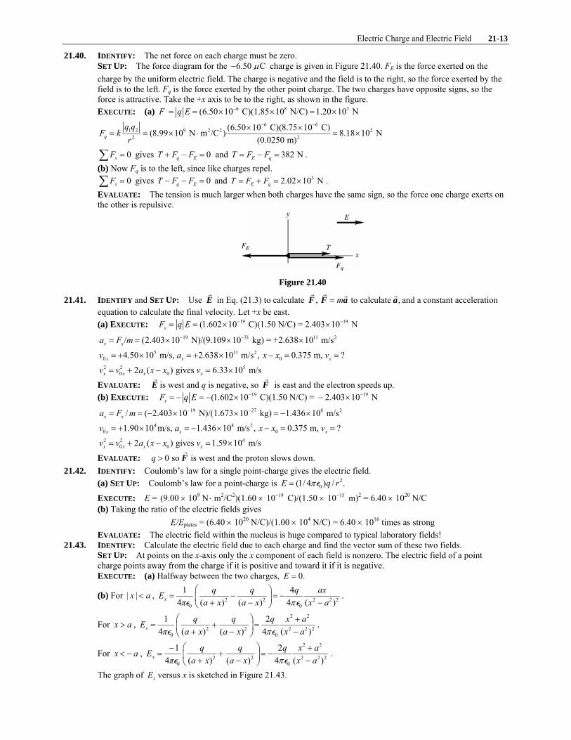
21.40. IDENTIFY: The net force on each charge must be zero. SET UP: The force diagram for the 6.50 Cμ− charge is given in Figure 21.40. FE is the force exerted on the charge by the uniform electric field. The charge is negative and the field is to the right, so the force exerted by the field is to the left. Fq is the force exerted by the other point charge. The two charges have opposite signs, so the force is attractive. Take the +x axis to be to the right, as shown in the figure. EXECUTE: (a) 6 8 3(6.50 10 C)(1.85 10 N/C) 1.20 10 NF q E −= = × × = ×
6 61 2 9 2 2 2
2 2
(6.50 10 C)(8.75 10 C)(8.99 10 N m /C ) 8.18 10 N(0.0250 m)q
q qF k
r
− −× ×= = × ⋅ = ×
0xF =∑ gives 0q ET F F+ − = and 382 NE qT F F= − = . (b) Now Fq is to the left, since like charges repel.
0xF =∑ gives 0q ET F F− − = and 32.02 10 NE qT F F= + = × . EVALUATE: The tension is much larger when both charges have the same sign, so the force one charge exerts on the other is repulsive.
Figure 21.40
21.41. IDENTIFY and SET UP: Use E in Eq. (21.3) to calculate , to calculate ,m=F F a a and a constant acceleration equation to calculate the final velocity. Let +x be east. (a) EXECUTE: 19 19(1.602 10 C)(1.50 N/C) = 2.403 10 NxF q E − −= = × ×
19 31 11 2/ (2.403 10 N)/(9.109 10 kg) = +2.638 10 m/sx xa F m − −= = × × × 5 11 2
0 04.50 10 m/s, 2.638 10 m/s , 0.375 m, ?x x xv a x x v= + × = + × − = = 2 2 5
0 02 ( ) gives 6.33 10 m/sx x x xv v a x x v= + − = ×
EVALUATE: E is west and q is negative, so F is east and the electron speeds up. (b) EXECUTE: 19 19(1.602 10 C)(1.50 N/C) = 2.403 10 NxF q E − −= − = − × − ×
19 27 8 2/ ( 2.403 10 N)/(1.673 10 kg) 1.436 10 m/sx xa F m − −= = − × × = − × 4 8 2
0 01.90 10 m/s, 1.436 10 m/s , 0.375 m, ?x x xv a x x v= + × = − × − = = 2 2 4
0 02 ( ) gives 1.59 10 m/sx x x xv v a x x v= + − = ×
EVALUATE: 0 so q > F is west and the proton slows down. 21.42. IDENTIFY: Coulomb’s law for a single point-charge gives the electric field.
(a) SET UP: Coulomb’s law for a point-charge is 20(1/ 4 ) / .E q rπ= P
EXECUTE: E = (9.00 × 10⁹ N ⋅ m2/C2)(1.60 × 1910− C)/(1.50 × 1510− m)2 = 6.40 × 10²⁰ N/C (b) Taking the ratio of the electric fields gives
E/Eplates = (6.40 × 10²⁰ N/C)/(1.00 × 104 N/C) = 6.40 × 10¹⁶ times as strong EVALUATE: The electric field within the nucleus is huge compared to typical laboratory fields!
21.43. IDENTIFY: Calculate the electric field due to each charge and find the vector sum of these two fields. SET UP: At points on the x-axis only the x component of each field is nonzero. The electric field of a point charge points away from the charge if it is positive and toward it if it is negative. EXECUTE: (a) Halfway between the two charges, 0.E =
(b) For | |x a< , 2 2 2 2 20 0
1 44 ( ) ( ) 4 ( )x
q q q axEπ a x a x x aπ
⎛ ⎞= − = −⎜ ⎟+ − −⎝ ⎠P P
.
For x a> , 2 2
2 2 2 2 20 0
1 24 ( ) ( ) 4 ( )x
q q q x aEπ a x a x x aπ
⎛ ⎞ += + =⎜ ⎟+ − −⎝ ⎠P P
.
For x a< − , 2 2
2 2 2 2 20 0
1 24 ( ) ( ) 4 ( )x
q q q x aEπ a x a x x aπ
⎛ ⎞− += + = −⎜ ⎟+ − −⎝ ⎠P P
.
The graph of xE versus x is sketched in Figure 21.43.

21-14 Chapter 21
EVALUATE: The magnitude of the field approaches infinity at the location of one of the point charges.
Figure 21.43
21.44. IDENTIFY: For a point charge, 2
qE k
r= . For the net electric field to be zero, 1E and 2E must have equal
magnitudes and opposite directions. SET UP: Let 1 0.500 nCq = + and 2 8.00 nC.q = + E is toward a negative charge and away from a positive charge. EXECUTE: The two charges and the directions of their electric fields in three regions are shown in Figure 21.44. Only in region II are the two electric fields in opposite directions. Consider a point a distance x from 1q so a
distance 1.20 m x− from 2q . 1 2E E= gives 2 2
0.500 nC 8.00 nC(1.20 )
k kx x
=−
. 2 216 (1.20 m )x x= − . 4 (1.20 m )x x= ± −
and 0.24 mx = is the positive solution. The electric field is zero at a point between the two charges, 0.24 m from the 0.500 nC charge and 0.96 m from the 8.00 nC charge. EVALUATE: There is only one point along the line connecting the two charges where the net electric field is zero. This point is closer to the charge that has the smaller magnitude.
Figure 21.44
21.45. IDENTIFY: Eq.(21.7) gives the electric field of each point charge. Use the principle of superposition and add the electric field vectors. In part (b) use Eq.(21.3) to calculate the force, using the electric field calculated in part (a). (a) SET UP: The placement of charges is sketched in Figure 21.45a.
Figure 21.45a
The electric field of a point charge is directed away from the point charge if the charge is positive and toward the
point charge if the charge is negative. The magnitude of the electric field is 20
1 ,4
qE
rπ=
Pwhere r is the distance
between the point where the field is calculated and the point charge. (i) At point a the fields 1 1 2 2 of and of q qE E are directed as shown in Figure 21.45b.
Figure 21.45b

Electric Charge and Electric Field 21-15
EXECUTE: 9
1 9 2 21 2 2
0 1
1 2.00 10 C(8.988 10 N m /C ) 449.4 N/C4 (0.200 m)
qE
rπ
−×= = × ⋅ =
P
92 9 2 2
2 2 20 2
1 5.00 10 C(8.988 10 N m /C ) 124.8 N/C4 (0.600 m)
qE
rπ
−×= = × ⋅ =
P
1 1449.4 N/C, 0x yE E= =
2 2124.8 N/C, 0x yE E= =
1 2 449.4 N/C 124.8 N/C 574.2 N/Cx x xE E E= + = + + = +
1 2 0y y yE E E= + = The resultant field at point a has magnitude 574 N/C and is in the +x-direction. (ii) SET UP: At point b the fields 1 1 2 2of and of q qE E are directed as shown in Figure 21.45c.
Figure 21.45c
EXECUTE: ( )
91 9 2 2
1 220 1
1 2.00 10 C(8.988 10 N m /C ) 12.5 N/C4 1.20 m
qE
rπ
−×= = × ⋅ =
P
( )( )
92 9 2 2
2 220 2
1 5.00 10 C8.988 10 N m /C 280.9 N/C4 0.400 m
qE
rπ
−×= = × ⋅ =
P
1 112.5 N/C, 0x yE E= =
2 2280.9 N/C, 0x yE E= − =
1 2 12.5 N/C 280.9 N/C 268.4 N/Cx x xE E E= + = + − = −
1 2 0y y yE E E= + = The resultant field at point b has magnitude 268 N/C and is in the x− -direction. (iii) SET UP: At point c the fields 1 1 2 2of and of q qE E are directed as shown in Figure 21.45d.
Figure 21.45d
EXECUTE: ( )
91 9 2 2
1 220 1
1 2.00 10 C(8.988 10 N m /C ) 449.4 N/C4 0.200 m
qE
rπ
−×= = × ⋅ =
P
( )9
2 9 2 22 2 2
0 2
1 5.00 10 C8.988 10 N m /C 44.9 N/C4 (1.00 m)
qE
rπ
−×= = × ⋅ =
P
1 1449.4 N/C, 0x yE E= − =
2 244.9 N/C, 0x yE E= + =
1 2 449.4 N/C 44.9 N/C 404.5 N/Cx x xE E E= + = − + = −
1 2 0y y yE E E= + = The resultant field at point b has magnitude 404 N/C and is in the x− -direction. (b) SET UP: Since we have calculated E at each point the simplest way to get the force is to use .e= −F E EXECUTE: (i) 19 17(1.602 10 C)(574.2 N/C) 9.20 10 N, -directionF x− −= × = × −
(ii) 19 17(1.602 10 C)(268.4 N/C) 4.30 10 N, -directionF x− −= × = × +
(iii) 19 17(1.602 10 C)(404.5 N/C) 6.48 10 N, -directionF x− −= × = × + EVALUATE: The general rule for electric field direction is away from positive charge and toward negative charge. Whether the field is in the - or -directionx x+ − depends on where the field point is relative to the charge that produces the field. In part (a) the field magnitudes were added because the fields were in the same direction and in (b) and (c) the field magnitudes were subtracted because the two fields were in opposite directions. In part (b) we could have used Coulomb's law to find the forces on the electron due to the two charges and then added these force vectors, but using the resultant electric field is much easier.

21-16 Chapter 21
21.46. IDENTIFY: Apply Eq.(21.7) to calculate the field due to each charge and then require that the vector sum of the two fields to be zero. SET UP: The field of each charge is directed toward the charge if it is negative and away from the charge if it is positive . EXECUTE: The point where the two fields cancel each other will have to be closer to the negative charge, because it is smaller. Also, it can’t be between the two charges, since the two fields would then act in the same direction. We could use Coulomb’s law to calculate the actual values, but a simpler way is to note that the 8.00 nC charge is twice as large as the 4.00 nC− charge. The zero point will therefore have to be a factor of 2 farther from the 8.00 nC charge for the two fields to have equal magnitude. Calling x the distance from the –4.00 nC charge: 1.20 2x x+ = and 2.90 mx = . EVALUATE: This point is 4.10 m from the 8.00 nC charge. The two fields at this point are in opposite directions and have equal magnitudes.
21.47. IDENTIFY: 2
qE k
r= . The net field is the vector sum of the fields due to each charge.
SET UP: The electric field of a negative charge is directed toward the charge. Label the charges q1, q2 and q3, as shown in Figure 21.47a. This figure also shows additional distances and angles. The electric fields at point P are shown in Figure 21.47b. This figure also shows the xy coordinates we will use and the x and y components of the fields 1E , 2E and 3E .
EXECUTE: 6
9 2 2 61 3 2
5.00 10 C(8.99 10 N m /C ) 4.49 10 N/C(0.100 m)
E E−×
= = × ⋅ = ×
69 2 2 6
2 2
2.00 10 C(8.99 10 N m /C ) 4.99 10 N/C(0.0600 m)
E−×
= × ⋅ = ×
1 2 3 0y y y yE E E E= + + = and 71 2 3 2 12 cos53.1 1.04 10 N/Cx x x xE E E E E E= + + = + = ×°
71.04 10 N/CE = × , toward the 2.00 Cμ− charge. EVALUATE: The x-components of the fields of all three charges are in the same direction.
Figure 21.47
21.48. IDENTIFY: A positive and negative charge, of equal magnitude q, are on the x-axis, a distance a from the origin. Apply Eq.(21.7) to calculate the field due to each charge and then calculate the vector sum of these fields. SET UP: E due to a point charge is directed away from the charge if it is positive and directed toward the charge if it is negative.
EXECUTE: (a) Halfway between the charges, both fields are in the -directionx− and 20
1 2 ,4
qEaπ
=P
in the
-directionx− .
(b) 2 20
14 ( ) ( )x
q qEa x a xπ
⎛ ⎞−= −⎜ ⎟+ −⎝ ⎠P
for | |x a< . 2 20
14 ( ) ( )x
q qEa x a xπ
⎛ ⎞−= +⎜ ⎟+ −⎝ ⎠P
for x a> .
2 20
14 ( ) ( )x
q qEa x a xπ
⎛ ⎞−= −⎜ ⎟+ −⎝ ⎠P
for x a< − . xE is graphed in Figure 21.48.

Electric Charge and Electric Field 21-17
EVALUATE: At points on the x axis and between the charges, xE is in the -directionx− because the fields from both charges are in this direction. For x a< − and x a> + , the fields from the two charges are in opposite directions and the field from the closer charge is larger in magnitude.
Figure 21.48
21.49. IDENTIFY: The electric field of a positive charge is directed radially outward from the charge and has magnitude
20
1 .4
qE
rπ=
P The resultant electric field is the vector sum of the fields of the individual charges.
SET UP: The placement of the charges is shown in Figure 21.49a.
Figure 21.49a
EXECUTE: (a) The directions of the two fields are shown in Figure 21.49b.
1 2 20
1 with 0.150 m.4
qE E r
rπ= = =
P
2 1 0; 0, 0x yE E E E E= − = = =
Figure 21.49b (b) The two fields have the directions shown in Figure 21.49c.
1 2 , in the -directionE E E x= + +
Figure 21.49c 9
9 2 211 2 2
0 1
1 6.00 10 C(8.988 10 N m /C ) 2396.8 N/C4 (0.150 m)
qE
rπ
−×= = × ⋅ =
P
92 9 2 2
2 2 20 2
1 6.00 10 C(8.988 10 N m /C ) 266.3 N/C4 (0.450 m)
qE
rπ
−×= = × ⋅ =
P
1 2 2396.8 N/C 266.3 N/C 2660 N/C; 2260 N/C, 0x yE E E E E= + = + = = + =
21-18 Chapter 21
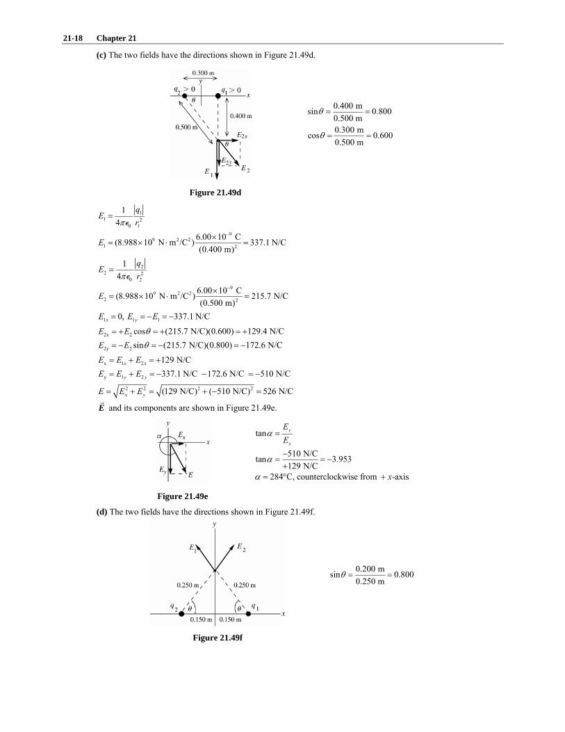
(c) The two fields have the directions shown in Figure 21.49d.
0.400 msin 0.8000.500 m
θ = =
0.300 mcos 0.6000.500 m
θ = =
Figure 21.49d
11 2
0 1
14
qE
rπ=
P
99 2 2
1 2
6.00 10 C(8.988 10 N m /C ) 337.1 N/C(0.400 m)
E−×
= × ⋅ =
22 2
0 2
14
qE
rπ=
P
99 2 2
2 2
6.00 10 C(8.988 10 N m /C ) 215.7 N/C(0.500 m)
E−×
= × ⋅ =
1 1 10, 337.1 N/Cx yE E E= = − = −
2x 2 cos (215.7 N/C)(0.600) 129.4 N/CE E θ= + = + = +
2y 2 sin (215.7 N/C)(0.800) 172.6 N/CE E θ= − = − = −
x 1 2 129 N/Cx xE E E= + = +
y 1 2 337.1 N/C 172.6 N/C 510 N/Cy yE E E= + = − − = − 2 2 2 2(129 N/C) ( 510 N/C) 526 N/Cx yE E E= + = + − =
E and its components are shown in Figure 21.49e.
tan y
x
EE
α =
510 N/Ctan 3.953129 N/C
α −= = −+
284 C, counterclockwise from -axisxα = ° +
Figure 21.49e (d) The two fields have the directions shown in Figure 21.49f.
0.200 msin 0.8000.250 m
θ = =
Figure 21.49f
Electric Charge and Electric Field 21-19
The components of the two fields are shown in Figure 21.49g.
1 2 20
14
qE E
rπ= =
P
99 2 2
1 2
6.00 10 C(8.988 10 N m /C )(0.250 m)
E−×
= × ⋅
1 2 862.8 N/CE E= =
Figure 21.49g
1 1 2 2cos , cosx xE E E Eθ θ= − = +
1 2 0x x xE E E= + =
1 1 2 2sin , siny yE E E Eθ θ= + = + ( )( )1 2 1 12 2 sin 2 862.8 N/C 0.800 1380 N/Cy y y yE E E E E θ= + = = = =
1380 N/C, in the -direction.E y= + EVALUATE: Point a is symmetrically placed between identical charges, so symmetry tells us the electric field must be zero. Point b is to the right of both charges and both electric fields are in the +x-direction and the resultant field is in this direction. At point c both fields have a downward component and the field of 2q has a component to the right, so the net E is in the 4th quadrant. At point d both fields have an upward component but by symmetry they have equal and opposite x-components so the net field is in the +y-direction. We can use this sort of reasoning to deduce the general direction of the net field before doing any calculations.
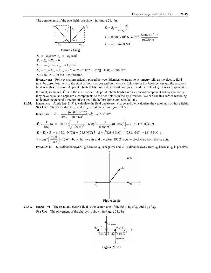
21.50. IDENTIFY: Apply Eq.(21.7) to calculate the field due to each charge and then calculate the vector sum of those fields. SET UP: The fields due to 1q and to 2q are sketched in Figure 21.50.
EXECUTE: 9
2 20
1 (6.00 10 C) ˆ ˆ( ) 150 N/C4 (0.6 m)π
−×= − = −E i i
P.
91 2 2
0
1 1 1ˆ ˆ ˆ ˆ(4.00 10 C) (0.600) (0.800) (21.6 28.8 ) N C4 (1.00 m) (1.00 m)π
− ⎛ ⎞= × + =⎜ ⎟
⎝ ⎠E i j i + j
P.
1 2ˆ ˆ( 128.4 N/C) (28.8 N/C)= −E = E + E i + j . 2 2(128.4 N/C) (28.8 N/C) 131.6 N/CE = + = at
1 28.8tan 12.6128.4
θ − ⎛ ⎞= = °⎜ ⎟⎝ ⎠
above the x− axis and therefore 196.2° counterclockwise from the +x axis.
EVALUATE: 1E is directed toward 1q because 1q is negative and 2E is directed away from 2q because 2q is positive.
Figure 21.50
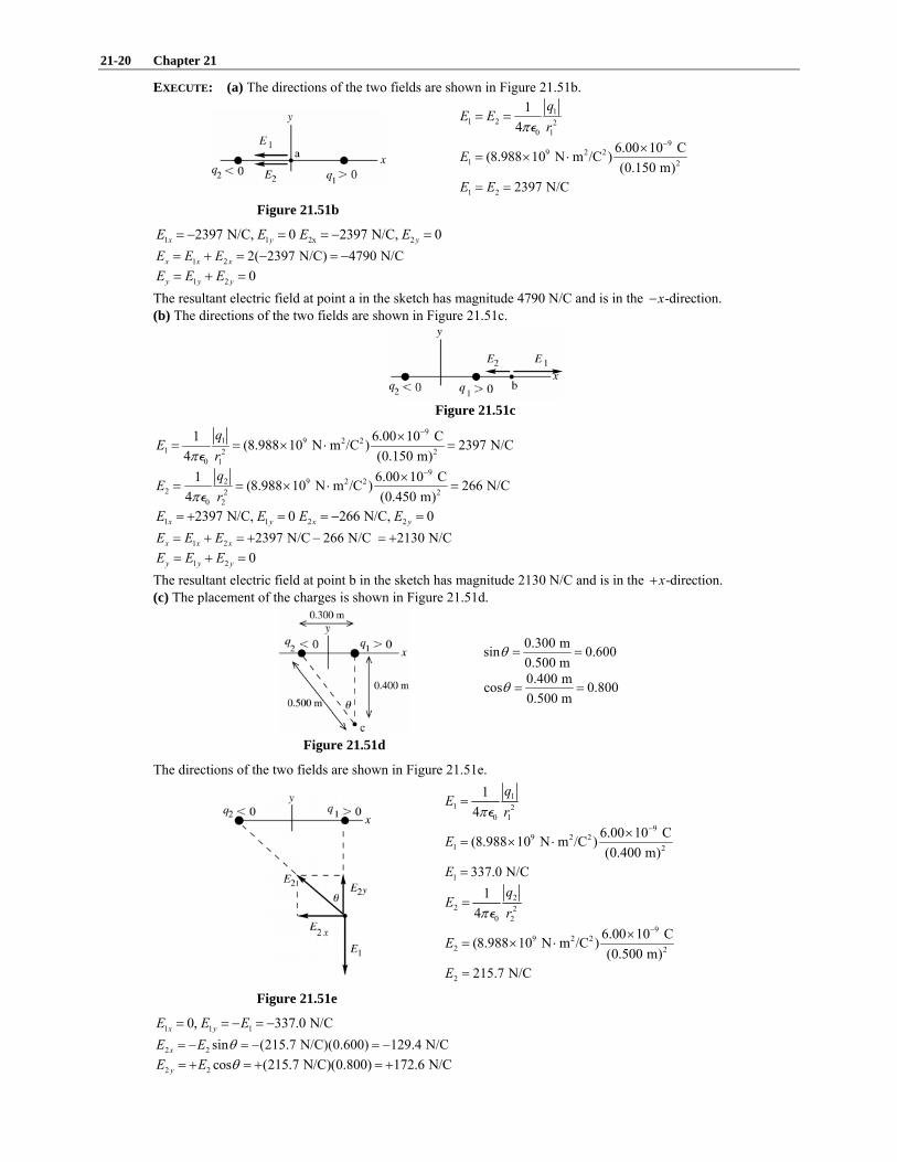
21.51. IDENTIFY: The resultant electric field is the vector sum of the field 1 1 2 2of and of .q qE E SET UP: The placement of the charges is shown in Figure 21.51a.
Figure 21.51a
21-20 Chapter 21
EXECUTE: (a) The directions of the two fields are shown in Figure 21.51b.
11 2 2
0 1
14
qE E
rπ= =
P
99 2 2
1 2
6.00 10 C(8.988 10 N m /C )(0.150 m)
E−×
= × ⋅
1 2 2397 N/CE E= =
Figure 21.51b
1 1 2x 22397 N/C, 0 2397 N/C, 0x y yE E E E= − = = − =
1 2 2( 2397 N/C) 4790 N/Cx x xE E E= + = − = −
1 2 0y y yE E E= + = The resultant electric field at point a in the sketch has magnitude 4790 N/C and is in the -direction.x− (b) The directions of the two fields are shown in Figure 21.51c.
Figure 21.51c
91 9 2 2
1 2 20 1
1 6.00 10 C(8.988 10 N m /C ) 2397 N/C4 (0.150 m)
qE
rπ
−×= = × ⋅ =
P
92 9 2 2
2 2 20 2
1 6.00 10 C(8.988 10 N m /C ) 266 N/C4 (0.450 m)
qE
rπ
−×= = × ⋅ =
P
1 1 2 22397 N/C, 0 266 N/C, 0x y x yE E E E= + = = − =
1 2 2397 N/C 266 N/C 2130 N/Cx x xE E E= + = + − = +
1 2 0y y yE E E= + = The resultant electric field at point b in the sketch has magnitude 2130 N/C and is in the -direction.x+ (c) The placement of the charges is shown in Figure 21.51d.
0.300 msin 0.6000.500 m
θ = =
0.400 mcos 0.8000.500 m
θ = =
Figure 21.51d The directions of the two fields are shown in Figure 21.51e.
11 2
0 1
14
qE
rπ=
P
99 2 2
1 2
6.00 10 C(8.988 10 N m /C )(0.400 m)
E−×
= × ⋅
1 337.0 N/CE =
22 2
0 2
14
qE
rπ=
P
99 2 2
2 2
6.00 10 C(8.988 10 N m /C )(0.500 m)
E−×
= × ⋅
2 215.7 N/CE =
Figure 21.51e
1 1 10, 337.0 N/Cx yE E E= = − = −
2 2 sin (215.7 N/C)(0.600) 129.4 N/CxE E θ= − = − = −
2 2 cos (215.7 N/C)(0.800) 172.6 N/CyE E θ= + = + = +
Electric Charge and Electric Field 21-21
1 2 129 N/Cx x xE E E= + = −
1 2 337.0 N/C 172.6 N/C 164 N/Cy y yE E E= + = − + = − 2 2 209 N/Cx yE E E= + =
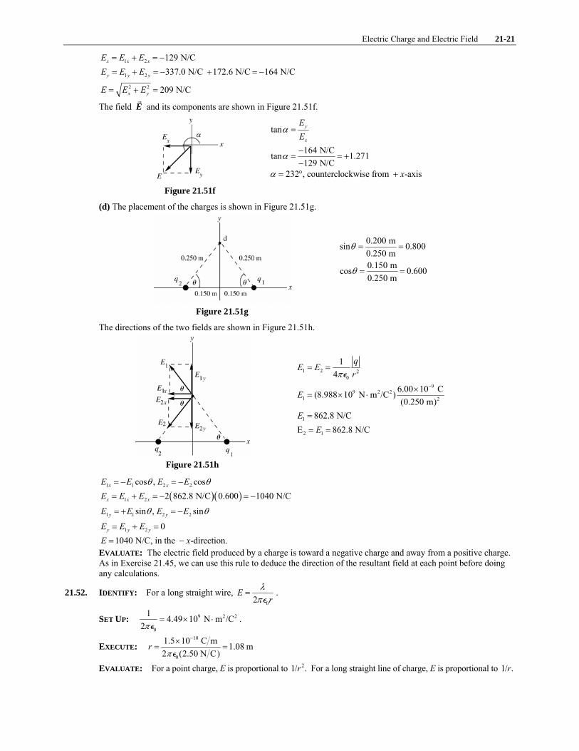
The field E and its components are shown in Figure 21.51f.
tan y
x
EE
α =
164 N/Ctan 1.271129 N/C
α −= = +−
232 , counterclockwise from -axisxα = ° +
Figure 21.51f (d) The placement of the charges is shown in Figure 21.51g.
0.200 msin 0.8000.250 m
θ = =
0.150 mcos 0.6000.250 m
θ = =
Figure 21.51g The directions of the two fields are shown in Figure 21.51h.
1 2 20
14
qE E
rπ= =
P
99 2 2
1 2
6.00 10 C(8.988 10 N m /C )(0.250 m)
E−×
= × ⋅
1 862.8 N/CE =
2 1E 862.8 N/CE= =
Figure 21.51h
1 1 2 2cos , cosx xE E E Eθ θ= − = −
( )( )1 2 2 862.8 N/C 0.600 1040 N/Cx x xE E E= + = − = −
1 1 2 2sin , siny yE E E Eθ θ= + = −
1 2 0y y yE E E= + = 1040 N/C, in the -direction.E x= −
EVALUATE: The electric field produced by a charge is toward a negative charge and away from a positive charge. As in Exercise 21.45, we can use this rule to deduce the direction of the resultant field at each point before doing any calculations.
21.52. IDENTIFY: For a long straight wire, 02
Er
λπ
=P
.
SET UP: 9 2 2
0
1 4.49 10 N m /C2π
= × ⋅P
.
EXECUTE: 10
0
1.5 10 C m 1.08 m2 (2.50 N C)
rπ
−×= =
P
EVALUATE: For a point charge, E is proportional to 21/ .r For a long straight line of charge, E is proportional to 1/ .r
21-22 Chapter 21
21.53. IDENTIFY: Apply Eq.(21.10) for the finite line of charge and 02
E λπ
=P
for the infinite line of charge.
SET UP: For the infinite line of positive charge, E is in the +x direction. EXECUTE: (a) For a line of charge of length 2a centered at the origin and lying along the y-axis, the electric field
is given by Eq.(21.10): 2 2
0
1 ˆ2 1x x a
λπ +
E = iP
.
(b) For an infinite line of charge: 0
ˆ2 xλπ
E = iP
. Graphs of electric field versus position for both distributions of
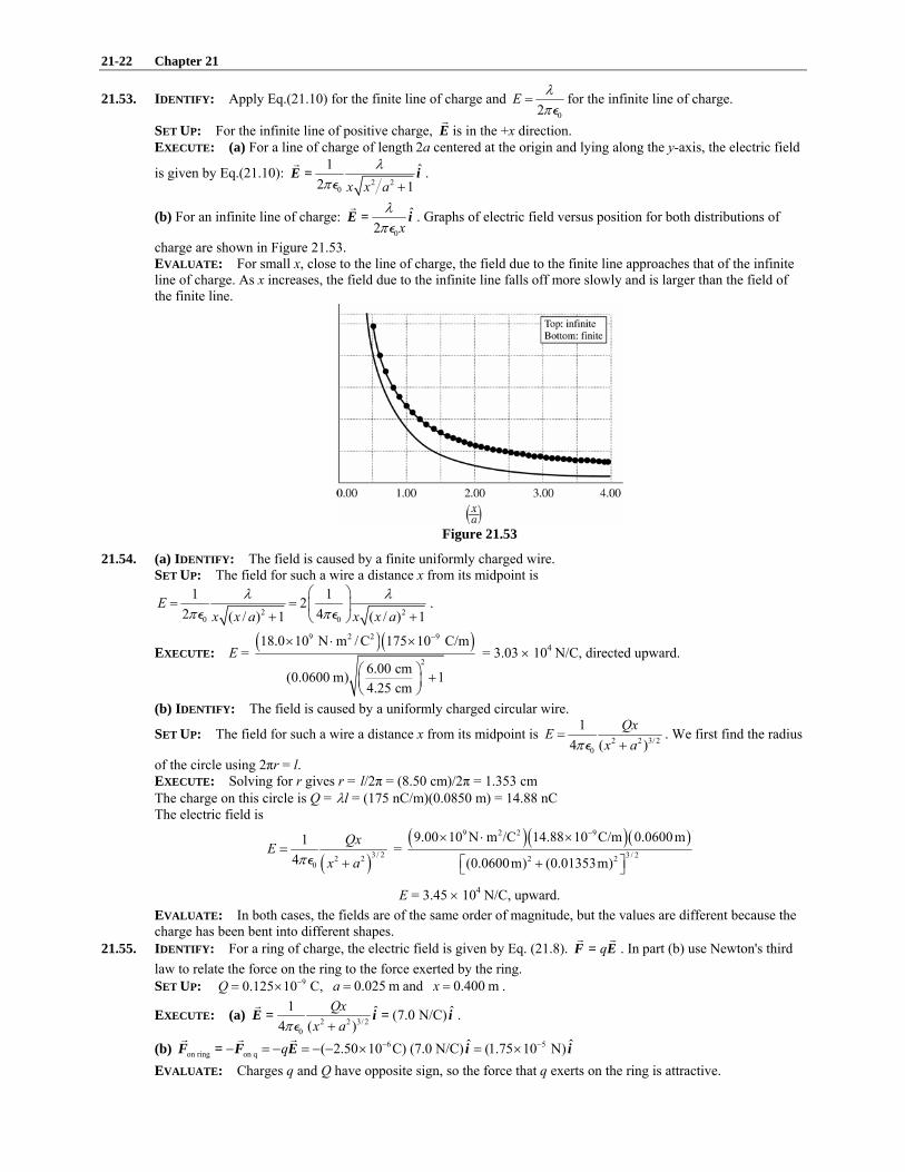
charge are shown in Figure 21.53. EVALUATE: For small x, close to the line of charge, the field due to the finite line approaches that of the infinite line of charge. As x increases, the field due to the infinite line falls off more slowly and is larger than the field of the finite line.
Figure 21.53
21.54. (a) IDENTIFY: The field is caused by a finite uniformly charged wire. SET UP: The field for such a wire a distance x from its midpoint is
2 20 0
1 122 4( / ) 1 ( / ) 1
Ex x a x x a
λ λπ π
⎛ ⎞= = ⎜ ⎟
+ +⎝ ⎠P P.
EXECUTE: E = ( )( )9 2 2 9
2
18.0 10 N m / C 175 10 C/m
6.00 cm(0.0600 m) 14.25 cm
−× ⋅ ×
⎛ ⎞ +⎜ ⎟⎝ ⎠
= 3.03 × 10⁴ N/C, directed upward.
(b) IDENTIFY: The field is caused by a uniformly charged circular wire.
SET UP: The field for such a wire a distance x from its midpoint is 2 2 3/20
14 ( )
QxEx aπ
=+P
. We first find the radius
of the circle using 2πr = l. EXECUTE: Solving for r gives r = l/2π = (8.50 cm)/2π = 1.353 cm The charge on this circle is Q = λl = (175 nC/m)(0.0850 m) = 14.88 nC The electric field is
( )3 / 22 20
14
QxEx aπ
=+P
= ( )( )( )9 2 2 9
3 / 22 2
9.00 10 N m /C 14.88 10 C/m 0.0600 m
(0.0600 m) (0.01353 m)
−× ⋅ ×
⎡ ⎤+⎣ ⎦
E = 3.45 × 10⁴ N/C, upward. EVALUATE: In both cases, the fields are of the same order of magnitude, but the values are different because the charge has been bent into different shapes.
21.55. IDENTIFY: For a ring of charge, the electric field is given by Eq. (21.8). qF = E . In part (b) use Newton's third law to relate the force on the ring to the force exerted by the ring. SET UP: 90.125 10 C,Q −= × 0.025 ma = and 0.400 mx = .
EXECUTE: (a) 2 2 3/ 20
1 ˆ ˆ(7.0 N/C)4 ( )
Qxx aπ +
E = i = iP
.
(b) 6 5on ring on q
ˆ ˆ( 2.50 10 C) (7.0 N/C) (1.75 10 N)q − −− = − = − − × = ×F = F E i i EVALUATE: Charges q and Q have opposite sign, so the force that q exerts on the ring is attractive.

Electric Charge and Electric Field 21-23
21.56. IDENTIFY: We must use the appropriate electric field formula: a uniform disk in (a), a ring in (b) because all the charge is along the rim of the disk, and a point-charge in (c). (a) SET UP: First find the surface charge density (Q/A), then use the formula for the field due to a disk of charge,
20
112 ( / ) 1
xER x
σ ⎡ ⎤= −⎢ ⎥
⎢ ⎥+⎣ ⎦P.
EXECUTE: The surface charge density is 9
2 2
6.50 10 C(0.0125 m)
Q QA r
σπ π
−×= = = = 1.324 × 510− C/m2.
The electric field is
20
112 ( / ) 1
xER x
σ ⎡ ⎤= −⎢ ⎥
⎢ ⎥+⎣ ⎦P =
5 2
12 2 2 2
1.324 10 C/m 112(8.85 10 C /N m ) 1.25 cm 1
2.00 cm
−
−
× ⎡ ⎤−⎢ ⎥× ⋅ ⎛ ⎞⎢ ⎥+⎜ ⎟⎢ ⎥⎝ ⎠⎣ ⎦
Ex = 1.14 × 10⁵ N/C, toward the center of the disk.
(b) SET UP: For a ring of charge, the field is ( )3 / 22 2
0
14
QxEx aπ
=+P
.
EXECUTE: Substituting into the electric field formula gives
( )3 / 22 20
14
QxEx aπ
=+P
= 9 2 2 9
3 / 22 2
(9.00 10 N m /C )(6.50 10 C)(0.0200 m)
(0.0200 m) (0.0125 m)
−× ⋅ ×
⎡ ⎤+⎣ ⎦
E = 8.92 × 10⁴ N/C, toward the center of the disk.
(c) SET UP: For a point charge, ( ) 201/ 4 / .E q rπ= P
EXECUTE: E = (9.00 × 10⁹ N ⋅ m2/C2)(6.50 × 910− C)/(0.0200 m)2 = 1.46 × 10⁵ N/C (d) EVALUATE: With the ring, more of the charge is farther from P than with the disk. Also with the ring the component of the electric field parallel to the plane of the ring is greater than with the disk, and this component cancels. With the point charge in (c), all the field vectors add with no cancellation, and all the charge is closer to point P than in the other two cases.
21.57. IDENTIFY: By superposition we can add the electric fields from two parallel sheets of charge. SET UP: The field due to each sheet of charge has magnitude 0/ 2σ P and is directed toward a sheet of negative charge and away from a sheet of positive charge. (a) The two fields are in opposite directions and 0.E = (b) The two fields are in opposite directions and 0.E =
(c) The fields of both sheets are downward and 0 0
22
E σ σ= =
P P, directed downward.
EVALUATE: The field produced by an infinite sheet of charge is uniform, independent of distance from the sheet. 21.58. IDENTIFY and SET UP: The electric field produced by an infinite sheet of charge with charge density σ has
magnitude 02
Eσ
=P
. The field is directed toward the sheet if it has negative charge and is away from the sheet if it
has positive charge. EXECUTE: (a) The field lines are sketched in Figure 21.58a. (b) The field lines are sketched in Figure 21.58b. EVALUATE: The spacing of the field lines indicates the strength of the field. In part (a) the two fields add between the sheets and subtract in the regions to the left of A and to the right of B. In part (b) the opposite is true.
Figure 21.58

21-24 Chapter 21
21.59. IDENTIFY: The force on the particle at any point is always tangent to the electric field line at that point. SET UP: The instantaneous velocity determines the path of the particle. EXECUTE: In Fig.21.29a the field lines are straight lines so the force is always in a straight line and velocity and acceleration are always in the same direction. The particle moves in a straight line along a field line, with increasing speed. In Fig.21.29b the field lines are curved. As the particle moves its velocity and acceleration are not in the same direction and the trajectory does not follow a field line. EVALUATE: In two-dimensional motion the velocity is always tangent to the trajectory but the velocity is not always in the direction of the net force on the particle.
21.60. IDENTIFY: The field appears like that of a point charge a long way from the disk and an infinite sheet close to the disk’s center. The field is symmetrical on the right and left. SET UP: For a positive point charge, E is proportional to 1/r 2 and is directed radially outward. For an infinite sheet of positive charge, the field is uniform and is directed away from the sheet. EXECUTE: The field is sketched in Figure 21.60. EVALUATE: Near the disk the field lines are parallel and equally spaced, which corresponds to a uniform field. Far from the disk the field lines are getting farther apart, corresponding to the 1/r 2 dependence for a point charge.
Figure 21.60
21.61. IDENTIFY: Use symmetry to deduce the nature of the field lines. (a) SET UP: The only distinguishable direction is toward the line or away from the line, so the electric field lines are perpendicular to the line of charge, as shown in Figure 21.61a.
Figure 21.61a
(b) EXECUTE and EVALUATE: The magnitude of the electric field is inversely proportional to the spacing of the field lines. Consider a circle of radius r with the line of charge passing through the center, as shown in Figure 21.61b.
Figure 21.61b
The spacing of field lines is the same all around the circle, and in the direction perpendicular to the plane of the circle the lines are equally spaced, so E depends only on the distance r. The number of field lines passing out through the circle is independent of the radius of the circle, so the spacing of the field lines is proportional to the reciprocal of the circumference 2 rπ of the circle. Hence E is proportional to 1/r.
21.62. IDENTIFY: Field lines are directed away from a positive charge and toward a negative charge. The density of field lines is proportional to the magnitude of the electric field. SET UP: The field lines represent the resultant field at each point, the net field that is the vector sum of the fields due to each of the three charges. EXECUTE: (a) Since field lines pass from positive charges and toward negative charges, we can deduce that the top charge is positive, middle is negative, and bottom is positive. (b) The electric field is the smallest on the horizontal line through the middle charge, at two positions on either side where the field lines are least dense. Here the y-components of the field are cancelled between the positive charges and the negative charge cancels the x-component of the field from the two positive charges. EVALUATE: Far from all three charges the field is the same as the field of a point charge equal to the algebraic sum of the three charges.
Electric Charge and Electric Field 21-25
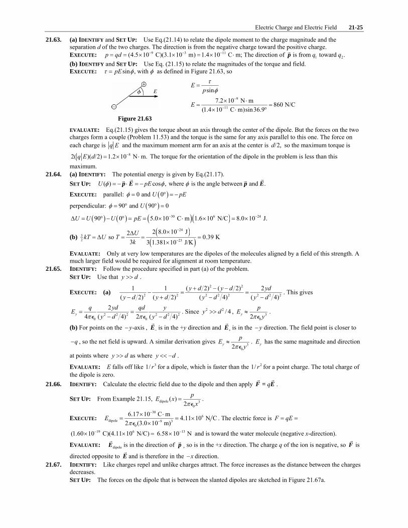
21.63. (a) IDENTIFY and SET UP: Use Eq.(21.14) to relate the dipole moment to the charge magnitude and the separation d of the two charges. The direction is from the negative charge toward the positive charge. EXECUTE: 9 3 11
1 2(4.5 10 C)(3.1 10 m) 1.4 10 C m; The direction of is from toward .p qd q q− − −= = × × = × ⋅ p (b) IDENTIFY and SET UP: Use Eq. (21.15) to relate the magnitudes of the torque and field. EXECUTE: sin , with pEτ φ φ= as defined in Figure 21.63, so
sinE
pτφ
=
9
11
7.2 10 N m 860 N/C(1.4 10 C m)sin36.9
E−
−
× ⋅= =
× ⋅ °
Figure 21.63 EVALUATE: Eq.(21.15) gives the torque about an axis through the center of the dipole. But the forces on the two charges form a couple (Problem 11.53) and the torque is the same for any axis parallel to this one. The force on each charge is q E and the maximum moment arm for an axis at the center is /2,d so the maximum torque is
82( )( /2) 1.2 10 N m.q E d −= × ⋅ The torque for the orientation of the dipole in the problem is less than this maximum.
21.64. (a) IDENTIFY: The potential energy is given by Eq.(21.17). SET UP: ( ) cos , where is the angle between and .U pEφ φ φ= − ⋅ = −p E p E
EXECUTE: parallel: ( )0 and 0U pEφ = ° = −
perpendicular: ( )90 and 90 0Uφ = ° ° =
( ) ( ) ( )( )30 6 2490 0 5.0 10 C m 1.6 10 N/C 8.0 10 J.U U U pE − −Δ = ° − ° = = × ⋅ × = ×
(b) ( )
( )24
32 23
2 8.0 10 J2 so 0.39 K3 3 1.381 10 J/K
UkT U Tk
−
−
×Δ= Δ = = =
×
EVALUATE: Only at very low temperatures are the dipoles of the molecules aligned by a field of this strength. A much larger field would be required for alignment at room temperature.
21.65. IDENTIFY: Follow the procedure specified in part (a) of the problem. SET UP: Use that y d>> .
EXECUTE: (a) 2 2
2 2 2 2 2 2 2 2
1 1 ( 2) ( 2) 2( 2) ( 2) ( 4) ( 4)
y d y d ydy d y d y d y d
+ − −− = =
− + − −. This gives
2 2 2 2 2 20 0
24 ( 4) 2 ( 4)y
q yd qd yEy d y dπ π
= =− −P P
. Since 2 2 / 4y d>> , 302y
pEyπ
≈P
.
(b) For points on the -axisy− , −E is in the +y direction and +E is in the y− direction. The field point is closer to
q− , so the net field is upward. A similar derivation gives 302y
pEyπ
≈P
. yE has the same magnitude and direction
at points where y d>> as where y d<< − .
EVALUATE: E falls off like 31/ r for a dipole, which is faster than the 21/ r for a point charge. The total charge of the dipole is zero.
21.66. IDENTIFY: Calculate the electric field due to the dipole and then apply qF = E .
SET UP: From Example 21.15, dipole 30
( )2
pE xxπ
=P
.
EXECUTE: 30
6dipole 9 3
0
6.17 10 C m 4.11 10 N C2 (3.0 10 m)
Eπ
−
−
× ⋅= = ×
×P. The electric force is F qE= =
19 6(1.60 10 C)(4.11 10 N/C)−× × = 136.58 10 N−× and is toward the water molecule (negative x-direction).
EVALUATE: dipoleE is in the direction of p ¸ so is in the +x direction. The charge q of the ion is negative, so F is
directed opposite to E and is therefore in the x− direction. 21.67. IDENTIFY: Like charges repel and unlike charges attract. The force increases as the distance between the charges
decreases. SET UP: The forces on the dipole that is between the slanted dipoles are sketched in Figure 21.67a.

21-26 Chapter 21
EXECUTE: The forces are attractive because the + and − charges of the two dipoles are closest. The forces are toward the slanted dipoles so have a net upward component. In Figure 21.67b, adjacent dipoles charges of opposite sign are closer than charges of the same sign so the attractive forces are larger than the repulsive forces and the dipoles attract. EVALUATE: Each dipole has zero net charge, but because of the charge separation there is a non-zero force between dipoles.
Figure 21.67
21.68. IDENTIFY: Find the vector sum of the fields due to each charge in the dipole. SET UP: A point on the x-axis with coordinate x is a distance 2 2( / 2)r d x= + from each charge.
EXECUTE: (a) The magnitude of the field the due to each charge is 2 2 20 0
1 14 4 ( 2)
q qEr d xπ π
⎛ ⎞= = ⎜ ⎟+⎝ ⎠P P
,
where d is the distance between the two charges. The x-components of the forces due to the two charges are equal and oppositely directed and so cancel each other. The two fields have equal y-components,
so 2 20
2 12 sin4 ( 2)y
qE Ed x
θπ
⎛ ⎞= = ⎜ ⎟+⎝ ⎠P
, where θ is the angle below the x-axis for both fields. 2 2
2sin( 2)
dd x
θ =+
and dipole 2 2 2 2 3 22 20 0
2 1 24 ( 2) 4 (( 2) )( 2)
q d qdEd x d xd xπ π
⎛ ⎞⎛ ⎞⎛ ⎞⎜ ⎟= =⎜ ⎟⎜ ⎟⎜ ⎟+ ++⎝ ⎠⎝ ⎠ ⎝ ⎠P P
. The field is the y− direction.
(b) At large x, 2 2( 2)x d>> , so the expression in part (a) reduces to the approximation dipole 304
qdExπ
≈P
.
EVALUATE: Example 21.15 shows that at points on the +y axis far from the dipole, dipole 302
qdEyπ
≈P
. The
expression in part (b) for points on the x axis has a similar form. 21.69. IDENTIFY: The torque on a dipole in an electric field is given by τ = p× E .
SET UP: sinpEτ φ= , where φ is the angle between the direction of p and the direction of E . EXECUTE: (a) The torque is zero when p is aligned either in the same direction as E or in the opposite direction, as shown in Figure 21.69a. (b) The stable orientation is when p is aligned in the same direction as E . In this case a small rotation of the dipole results in a torque directed so as to bring p back into alignment with E . When p is directed opposite to E , a small displacement results in a torque that takes p farther from alignment with E . (c) Field lines for dipoleE in the stable orientation are sketched in Figure 21.69b. EVALUATE: The field of the dipole is directed from the + charge toward the − charge.
Figure 21.69
21.70. IDENTIFY: The plates produce a uniform electric field in the space between them. This field exerts torque on a dipole and gives it potential energy. SET UP: The electric field between the plates is given by 0/ ,E σ= P and the dipole moment is p = ed. The potential energy of the dipole due to the field is cosU pE φ= − ⋅ = −p E , and the torque the field exerts on it is τ = pE sin φ.

Electric Charge and Electric Field 21-27
EXECUTE: (a) The potential energy, cosU pE φ= − ⋅ = −p E , is a maximum when φ = 180°. The field between the plates is 0/ ,E σ= P giving
Umax = (1.60 × 10⁻¹⁹ C)(220 × 10–9 m)(125 × 10–6 C/m2)/(8.85 × 10–12 C2/N ⋅ m2) = 4.97 × 10⁻¹⁹ J The orientation is parallel to the electric field (perpendicular to the plates) with the positive charge of the dipole toward the positive plate. (b) The torque, τ = pE sin φ, is a maximum when φ = 90° or 270°. In this case
max 0 0/ /pE p edτ σ σ= = =P P
( )( )( ) ( )19 9 6 12 2 2max 1.60 10 C 220 10 m 125 10 C/m 8.85 10 C / N mτ − − − 2 −= × × × × ⋅
19max 4.97 10 N mτ −= × ⋅
The dipole is oriented perpendicular to the electric field (parallel to the plates). (c) F = 0. EVALUATE: When the potential energy is a maximum, the torque is zero. In both cases, the net force on the dipole is zero because the forces on the charges are equal but opposite (which would not be true in a nonuniform electric field).
21.71. (a) IDENTIFY: Use Coulomb's law to calculate each force and then add them as vectors to obtain the net force. Torque is force times moment arm. SET UP: The two forces on each charge in the dipole are shown in Figure 21.71a.
sin 1.50 / 2.00 so 48.6θ θ= = ° Opposite charges attract and like charges repel.
1 2 0x x xF F F= + =
Figure 21.71a
EXECUTE: 6 6
31 2 2
(5.00 10 C)(10.0 10 C) 1.124 10 N(0.0200 m)
qqF k k
r
− −′ × ×= = = ×
1 1 sin 842.6 NyF F θ= − = −
2 1 2842.6 N so 1680 Ny y y yF F F F= − = + = − (in the direction from the 5.00- Cμ+ charge toward the 5.00- Cμ− charge). EVALUATE: The x-components cancel and the y-components add. (b) SET UP: Refer to Figure 21.71b.
The y-components have zero moment arm and therefore zero torque.
1 2and x xF F both produce clockwise torques.
Figure 21.71b EXECUTE: 1 1 cos 743.1 NXF F θ= =
12( )(0.0150 m) 22.3 N m, clockwisexFτ = = ⋅ EVALUATE: The electric field produced by the 10.00 Cμ− charge is not uniform so Eq. (21.15) does not apply.

21-28 Chapter 21
21.72. IDENTIFY: Apply 2
qqF k
r′
= for each pair of charges and find the vector sum of the forces that 1q and 2q exert on 3.q
SET UP: Like charges repel and unlike charges attract. The three charges and the forces on 3q are shown in Figure 21.72.
Figure 21.72
EXECUTE: (a) 9 9
1 3 9 2 2 41 2 2
1
(5.00 10 C)(6.00 10 C)(8.99 10 N m /C ) 1.079 10 C(0.0500 m)
q qF k
r
− −−× ×
= = × ⋅ = × .
36.9θ = ° . 51 1 cos 8.63 10 NxF F θ −= + = × . 5
1 1 sin 6.48 10 NyF F θ −= + = × . 9 9
2 3 9 2 2 42 2 2
2
(2.00 10 C)(6.00 10 C)(8.99 10 N m /C ) 1.20 10 C(0.0300 m)
q qF k
r
− −−× ×
= = × ⋅ = × .
2 0xF = , 42 2 1.20 10 NyF F −= − = − × . 5
1 2 8.63 10 Nx x xF F F −= + = × . 5 4 5
1 2 6.48 10 N ( 1.20 10 N) 5.52 10 Ny y yF F F − − −= + = × + − × = − × .
(b) 2 2 41.02 10 Nx yF F F −= + = × . tan 0.640y
x
FF
φ = = . 32.6φ = ° , below the x+ axis.
EVALUATE: The individual forces on q3 are computed from Coulomb’s law and then added as vectors, using components.
21.73. (a) IDENTIFY: Use Coulomb's law to calculate the force exerted by each Q on q and add these forces as vectors to find the resultant force. Make the approximation x a>> and compare the net force to F kx= − to deduce k and then (1/ 2 ) / .f k mπ= SET UP: The placement of the charges is shown in Figure 21.73a.
Figure 21.73a
EXECUTE: Find the net force on q.
1 2 andx x xF F F= + 1 1 2 2, x xF F F F= + = −
Figure 21.73b
( ) ( )1 22 20 0
1 1, 4 4
qQ qQF Fa x a xπ π
= =+ −P P
( ) ( )1 2 2 20
1 14xqQF F F
a x a xπ⎡ ⎤= − = −⎢ ⎥+ −⎣ ⎦P
2 2
20
1 14x
qQ x xFa a aπ
− −⎡ ⎤⎛ ⎞ ⎛ ⎞= + + − −⎢ ⎥⎜ ⎟ ⎜ ⎟⎝ ⎠ ⎝ ⎠⎢ ⎥⎣ ⎦P

Electric Charge and Electric Field 21-29
Since x a<< we can use the binomial expansion for 2 2(1 / ) and (1 / )x a x a− −− + and keep only the first two terms:
(1 ) 1 .nz nz+ ≈ + For 2(1 / ) ,x a −− /z x a= − and 2n = − so 2(1 / ) 1 2 / .x a x a−− ≈ + For 2(1 / ) ,x a −+ /z x a= + and
2n = − so 2(1 / ) 1 2 / .x a x a−+ ≈ − Then 2 30 0
2 21 1 .4
qQ x x qQF xa a a aπ π
⎛ ⎞⎡ ⎤⎛ ⎞ ⎛ ⎞≈ − − + = −⎜ ⎟⎜ ⎟ ⎜ ⎟⎢ ⎥⎝ ⎠ ⎝ ⎠⎣ ⎦ ⎝ ⎠P P For simple harmonic
motion F kx= − and the frequency of oscillation is ( )1/ 2 / .f k mπ= The net force here is of this form, with
30/ .k qQ aπ= P Thus 3
0
1 .2
qQfmaπ π
=P
(b) The forces and their components are shown in Figure 21.73c.
Figure 21.73c
The x-components of the forces exerted by the two charges cancel, the y-components add, and the net force is in the +y-direction when y > 0 and in the -directiony− when y < 0. The charge moves away from the origin on the y-axis and never returns. EVALUATE: The directions of the forces and of the net force depend on where q is located relative to the other two charges. In part (a), 0 at 0F x= = and when the charge q is displaced in the +x- or –x-direction the net force is a restoring force, directed to return to 0.q x = The charge oscillates back and forth, similar to a mass on a spring.
21.74. IDENTIFY: Apply 0xF =∑ and 0yF =∑ to one of the spheres.
SET UP: The free-body diagram is sketched in Figure 21.74. eF is the repulsive Coulomb force between the spheres. For small ,θ sin tanθ θ≈ .
EXECUTE: esin 0xF T Fθ∑ = − = and cos 0yF T mgθ∑ = − = . So 2
e 2sin
cosmg kqF
dθ
θ = = . But tan sin 2dLθ θ≈ = ,
so 2
3 2kq Ld mg= and 1/32
02q Ld mgπ
⎛ ⎞= ⎜ ⎟⎝ ⎠P .
EVALUATE: d increases when q increases.
Figure 21.74
21.75. IDENTIFY: Use Coulomb's law for the force that one sphere exerts on the other and apply the 1st condition of equilibrium to one of the spheres. (a) SET UP: The placement of the spheres is sketched in Figure 21.75a.
Figure 21.75a
21-30 Chapter 21
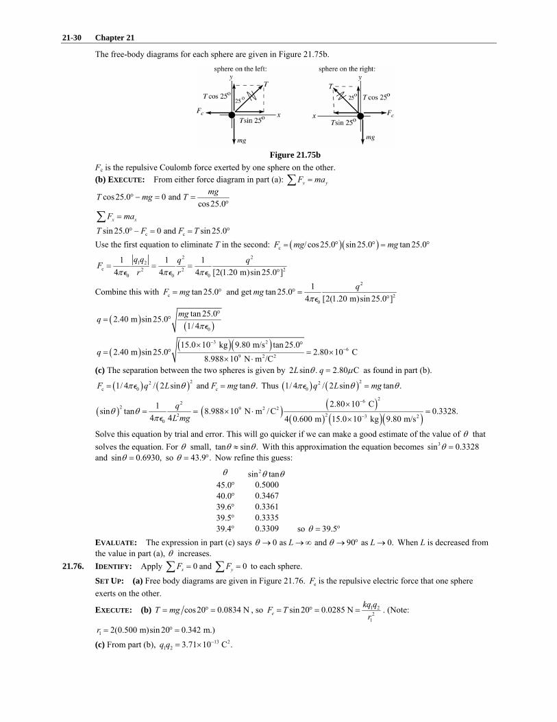
The free-body diagrams for each sphere are given in Figure 21.75b.
Figure 21.75b
Fc is the repulsive Coulomb force exerted by one sphere on the other. (b) EXECUTE: From either force diagram in part (a): y yF ma=∑
cos25.0 0 and cos25.0
mgT mg T° − = =°
x xF ma=∑
c csin 25.0 0 and sin 25.0T F F T° − = = ° Use the first equation to eliminate T in the second: ( )( )c / cos25.0 sin 25.0 tan 25.0F mg mg= ° ° = °
2 21 2
c 2 2 20 0 0
1 1 14 4 4 [2(1.20 m)sin 25.0 ]
q q q qFr rπ π π
= = =°P P P
Combine this with c tan 25.0F mg= ° and get2
20
1tan 25.04 [2(1.20 m)sin 25.0 ]
qmgπ
° =°P
( ) ( )0
tan 25.02.40 m sin 25.01/ 4
mgqπ
°= °
P
( ) ( )( )3 26
9 2 2
15.0 10 kg 9.80 m/s tan 25.02.40 m sin 25.0 2.80 10 C
8.988 10 N m /Cq
−−
× °= ° = ×
× ⋅
(c) The separation between the two spheres is given by 2 sin . 2.80 CL qθ μ= as found in part (b).
( ) ( )22c 0 c1/ 4 / 2 sin and tan .F q L F mgπ θ θ= =P Thus ( ) ( )22
01/ 4 / 2 sin tan .q L mgπ θ θ=P
( )2
22
0
1sin tan4 4
qL mg
θ θπ
= =P
( ) ( )( ) ( )( )
269 2 2
2 3 2
2.80 10 C8.988 10 N m / C 0.3328.
4 0.600 m 15.0 10 kg 9.80 m/s
−
−
×× ⋅ =
×
Solve this equation by trial and error. This will go quicker if we can make a good estimate of the value of θ that solves the equation. For θ small, tan sin .θ θ≈ With this approximation the equation becomes 3sin 0.3328θ = and sin 0.6930,θ = so 43.9 .θ = ° Now refine this guess:
θ 2sin tanθ θ 45.0° 0.5000 40.0° 0.3467 39.6° 0.3361 39.5° 0.3335 39.4° 0.3309 so 39.5θ = °
EVALUATE: The expression in part (c) says 0 as and 90 as 0.L Lθ θ→ →∞ → ° → When L is decreased from the value in part (a), θ increases.
21.76. IDENTIFY: Apply 0xF =∑ and 0yF =∑ to each sphere.
SET UP: (a) Free body diagrams are given in Figure 21.76. eF is the repulsive electric force that one sphere exerts on the other.
EXECUTE: (b) cos20 0.0834 NT mg= ° = , so 1 22
1
sin 20 0.0285 Nekq qF T
r= ° = = . (Note:
1 2(0.500 m)sin 20 0.342 m.)r = ° =
(c) From part (b), 13 21 2 3.71 10 C .q q −= ×
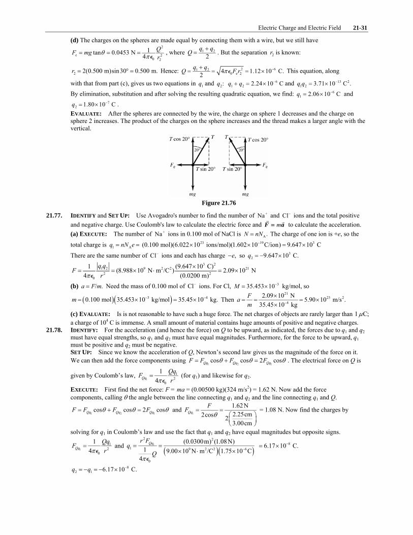
Electric Charge and Electric Field 21-31
(d) The charges on the spheres are made equal by connecting them with a wire, but we still have 2
e 20 2
1tan 0.0453 N 4QF mgr
θ π= = = P, where 1 2
2q qQ +
= . But the separation 2r is known:
2 2(0.500 m)sin30 0.500 m.r = ° = Hence: 2 61 20 e 24 1.12 10 C.2
q qQ F rπ −+= = = ×P This equation, along
with that from part (c), gives us two equations in 1q and 2:q 61 2 2.24 10 Cq q −+ = × and 13 2
1 2 3.71 10 C .q q −= × By elimination, substitution and after solving the resulting quadratic equation, we find: 6
1 2.06 10 Cq −= × and 7
2 1.80 10 Cq −= × . EVALUATE: After the spheres are connected by the wire, the charge on sphere 1 decreases and the charge on sphere 2 increases. The product of the charges on the sphere increases and the thread makes a larger angle with the vertical.
Figure 21.76
21.77. IDENTIFY and SET UP: Use Avogadro's number to find the number of +Na and Cl− ions and the total positive and negative charge. Use Coulomb's law to calculate the electric force and mF a= to calculate the acceleration. (a) EXECUTE: The number of +Na ions in 0.100 mol of NaCl is A.N nN= The charge of one ion is +e, so the
total charge is 1 Aq nN e= = 23 19 3(0.100 mol)(6.022 10 ions/mol)(1.602 10 C/ion) 9.647 10 C−× × = ×
There are the same number of Cl− ions and each has charge ,e− so 32 9.647 10 C.q = − ×
3 21 2 9 2 2 21
2 20
1 (9.647 10 C)(8.988 10 N m /C ) 2.09 10 N4 (0.0200 m)
q qF
rπ×
= = × ⋅ = ×P
(b) / .a F m= Need the mass of 0.100 mol of Cl− ions. For Cl, 335.453 10M −= × kg/mol, so
( )( )3 40.100 mol 35.453 10 kg/mol 35.45 10 kg.m − −= × = × Then 21
23 24
2.09 10 N 5.90 10 m/s .35.45 10 kg
Fam −
×= = = ×
×
(c) EVALUATE: Is is not reasonable to have such a huge force. The net charges of objects are rarely larger than 1 C;μ a charge of 104 C is immense. A small amount of material contains huge amounts of positive and negative charges.
21.78. IDENTIFY: For the acceleration (and hence the force) on Q to be upward, as indicated, the forces due to q1 and q2 must have equal strengths, so q1 and q2 must have equal magnitudes. Furthermore, for the force to be upward, q1 must be positive and q2 must be negative. SET UP: Since we know the acceleration of Q, Newton’s second law gives us the magnitude of the force on it. We can then add the force components using
1 2 1cos cos 2 cosQq Qq QqF F F Fθ θ θ= + = . The electrical force on Q is
given by Coulomb’s law, 1
12
0
14Qq
QqFrπ
=P
(for q1) and likewise for q2.
EXECUTE: First find the net force: F = ma = (0.00500 kg)(324 m/s2) = 1.62 N. Now add the force components, calling θ the angle between the line connecting q1 and q2 and the line connecting q1 and Q.
1 2 1cos cos 2 cosQq Qq QqF F F Fθ θ θ= + = and
1
1.62 N2.25 cm2cos 23.00 cm
QqFFθ
= =⎛ ⎞⎜ ⎟⎝ ⎠
= 1.08 N. Now find the charges by
solving for q1 in Coulomb’s law and use the fact that q1 and q2 have equal magnitudes but opposite signs.
1
12
0
14Qq
QqFrπ
=P
and ( )( )1
2 2
1 9 2 2 6
0
(0.0300 m) (1.08 N)1 9.00 10 N m /C 1.75 10 C
4
Qqr Fq
Qπ
−= =
× ⋅ ×P
86.17 10 C.−= ×
82 1 6.17 10 C.q q −= − = − ×
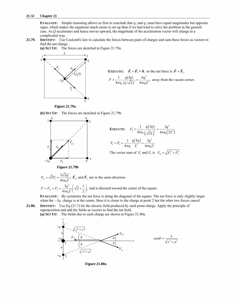
21-32 Chapter 21
EVALUATE: Simple reasoning allows us first to conclude that q1 and q2 must have equal magnitudes but opposite signs, which makes the equations much easier to set up than if we had tried to solve the problem in the general case. As Q accelerates and hence moves upward, the magnitude of the acceleration vector will change in a complicated way.
21.79. IDENTIFY: Use Coulomb's law to calculate the forces between pairs of charges and sum these forces as vectors to find the net charge. (a) SET UP: The forces are sketched in Figure 21.79a.
EXECUTE: 1 3 ,+ 0F F = so the net force is 2.=F F 2
220 0
1 (3 ) 6 ,4 4( / 2)
q q qFLLπ π
= =P P
away from the vacant corner.
Figure 21.79a (b) SET UP: The forces are sketched in Figure 21.79b.
EXECUTE: ( )( ) ( )
2
2 2 20 0
31 34 4 22
q q qFLLπ π
= =P P
( ) 2
1 3 2 20 0
31 34 4
q q qF FL Lπ π
= = =P P
The vector sum of 1 3and isF F 2 213 1 3 .F F F= +
Figure 21.79b 2
13 1 13 220
3 22 ; and 4
qF FLπ
= = F FP
are in the same direction.
2
13 2 20
3 12 ,4 2
qF F FLπ⎛ ⎞= + = +⎜ ⎟⎝ ⎠P
and is directed toward the center of the square.
EVALUATE: By symmetry the net force is along the diagonal of the square. The net force is only slightly larger when the 3q− charge is at the center. Here it is closer to the charge at point 2 but the other two forces cancel.
21.80. IDENTIFY: Use Eq.(21.7) for the electric field produced by each point charge. Apply the principle of superposition and add the fields as vectors to find the net field. (a) SET UP: The fields due to each charge are shown in Figure 21.80a.
2 2cos x
x aθ =
+
Figure 21.80a
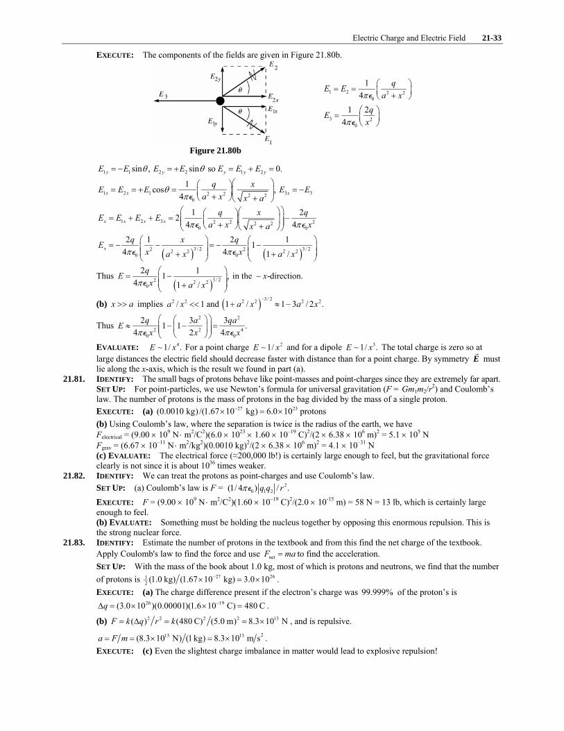
Electric Charge and Electric Field 21-33
EXECUTE: The components of the fields are given in Figure 21.80b.
1 2 2 20
14
qE Ea xπ
⎛ ⎞= = ⎜ ⎟+⎝ ⎠P
3 20
1 24
qExπ
⎛ ⎞= ⎜ ⎟⎝ ⎠P
Figure 21.80b
1 1 2 2 1 2sin , sin so 0.y y y y yE E E E E E Eθ θ= − = + = + =
1 2 1 3 32 2 2 20
1cos , 4x x x
q xE E E E Ea x x a
θπ
⎛ ⎞⎛ ⎞= = + = = −⎜ ⎟⎜ ⎟+⎝ ⎠ +⎝ ⎠P
1 2 3 2 2 22 20 0
1 224 4x x x x
q x qE E E Ea x xx aπ π
⎛ ⎞⎛ ⎞⎛ ⎞= + + = −⎜ ⎟⎜ ⎟⎜ ⎟⎜ ⎟+⎝ ⎠ +⎝ ⎠⎝ ⎠P P
( ) ( )3 / 2 3 / 22 22 2 2 20 0
2 1 2 114 4 1 /
xq x qE
x xa x a xπ π⎛ ⎞ ⎛ ⎞= − − = − −⎜ ⎟ ⎜ ⎟⎜ ⎟ ⎜ ⎟+ +⎝ ⎠ ⎝ ⎠
P P
Thus ( )3 / 22 2 2
0
2 11 , in the -direction.4 1 /
qE xx a xπ⎛ ⎞= − −⎜ ⎟⎜ ⎟+⎝ ⎠
P
(b) x a>> implies ( ) 3 / 22 2 2 2 2 2/ 1 and 1 / 1 3 / 2 .a x a x a x−
<< + ≈ −
Thus 2 2
2 2 40 0
2 3 31 1 .4 2 4
q a qaEx x xπ π⎛ ⎞⎛ ⎞
≈ − − =⎜ ⎟⎜ ⎟⎜ ⎟⎝ ⎠⎝ ⎠P P
EVALUATE: 41/ .E x∼ For a point charge 21/E x∼ and for a dipole 31/ .E x∼ The total charge is zero so at large distances the electric field should decrease faster with distance than for a point charge. By symmetry E must lie along the x-axis, which is the result we found in part (a).
21.81. IDENTIFY: The small bags of protons behave like point-masses and point-charges since they are extremely far apart. SET UP: For point-particles, we use Newton’s formula for universal gravitation (F = Gm1m2/r2) and Coulomb’s law. The number of protons is the mass of protons in the bag divided by the mass of a single proton. EXECUTE: (a) 27 23(0.0010 kg) /(1.67 10 kg) 6.0 10−× = × protons (b) Using Coulomb’s law, where the separation is twice is the radius of the earth, we have Felectrical = (9.00 × 10⁹ N ⋅ m2/C2)(6.0 × 1023 × 1.60 × 10–19 C)2/(2 × 6.38 × 106 m)2 = 5.1 × 10⁵ N Fgrav = (6.67 × 10⁻¹¹ N ⋅ m2/kg2)(0.0010 kg)2/(2 × 6.38 × 106 m)2 = 4.1 × 10⁻³¹ N (c) EVALUATE: The electrical force (≈200,000 lb!) is certainly large enough to feel, but the gravitational force clearly is not since it is about 1036 times weaker.
21.82. IDENTIFY: We can treat the protons as point-charges and use Coulomb’s law. SET UP: (a) Coulomb’s law is F = 2
0 1 2(1/ 4 ) / .q q rπP EXECUTE: F = (9.00 × 10⁹ N ⋅ m2/C2)(1.60 × 10–19 C)2/(2.0 × 10-15 m) = 58 N = 13 lb, which is certainly large enough to feel. (b) EVALUATE: Something must be holding the nucleus together by opposing this enormous repulsion. This is the strong nuclear force.
21.83. IDENTIFY: Estimate the number of protons in the textbook and from this find the net charge of the textbook. Apply Coulomb's law to find the force and use netF ma= to find the acceleration. SET UP: With the mass of the book about 1.0 kg, most of which is protons and neutrons, we find that the number of protons is 27 261
2 (1.0 kg) (1.67 10 kg) 3.0 10−× = × . EXECUTE: (a) The charge difference present if the electron’s charge was 99.999% of the proton’s is
26 19(3.0 10 )(0.00001)(1.6 10 C) 480 Cq −Δ = × × = .
(b) 2 2 2 2 13( ) (480 C) (5.0 m) 8.3 10 NF k q r k= Δ = = × , and is repulsive. 213 13(8.3 10 N) (1 kg) 8.3 10 m sa F m= = × = × .
EXECUTE: (c) Even the slightest charge imbalance in matter would lead to explosive repulsion!

21-34 Chapter 21
21.84. IDENTIFY: The electric field exerts equal and opposite forces on the two balls, causing them to swing away from each other. When the balls hang stationary, they are in equilibrium so the forces on them (electrical, gravitational, and tension in the strings) must balance. SET UP: (a) The force on the left ball is in the direction of the electric field, so it must be positive, while the force on the right ball is opposite to the electric field, so it must be negative. (b) Balancing horizontal and vertical forces gives qE = T sin θ/2 and mg = T cos θ/2. EXECUTE: Solving for the angle θ gives: θ = 2 arctan(qE/mg). (c) As E → ∞, θ → 2 arctan(∞) = 2 (π/2) = π = 180° EVALUATE: If the field were large enough, the gravitational force would not be important, so the strings would be horizontal.
21.85. IDENTIFY and SET UP: Use the density of copper to calculate the number of moles and then the number of atoms. Calculate the net charge and then use Coulomb's law to calculate the force.
EXECUTE: (a) ( ) ( )33 3 3 3 54 48.9 10 kg/m 1.00 10 m 3.728 10 kg3 3
m V rρ ρ π π − −⎛ ⎞ ⎛ ⎞= = = × × = ×⎜ ⎟ ⎜ ⎟⎝ ⎠ ⎝ ⎠
( ) ( )5 3 4/ 3.728 10 kg / 63.546 10 kg/mol 5.867 10 moln m M − − −= = × × = × 203.5 10 atomsAN nN= = ×
(b) ( )( )20 2229 3.5 10 1.015 10eN = × = × electrons and protons
( ) ( )( )( )2 19 22net 0.99900 0.100 10 1.602 10 C 1.015 10 1.6 Ce eq eN eN − −= − = × × × =
( )( )
2210
22
1.6 C2.3 10 N
1.00 mqF k kr
= = = ×
EVALUATE: The amount of positive and negative charge in even small objects is immense. If the charge of an electron and a proton weren't exactly equal, objects would have large net charges.
21.86. IDENTIFY: Apply constant acceleration equations to a drop to find the acceleration. Then use F ma= to find the force and F q E= to find q . SET UP: Let 2.0 cmD = be the horizontal distance the drop travels and 0.30 mmd = be its vertical displacement. Let +x be horizontal and in the direction from the nozzle toward the paper and let +y be vertical, in the direction of the deflection of the drop. 0xa = and ya a= .
EXECUTE: First, the mass of the drop: 6 3
3 114 (15.0 10 m)(1000 kg m ) 1.41 10 kg3
m V πρ−
−⎛ ⎞×= = = ×⎜ ⎟
⎝ ⎠. Next, the
time of flight: (0.020 m) (20 m/s) 0.00100 st D v= = = . 212
d at= . 4
22 2
2 2(3.00 10 m) 600 m s(0.001s)
dat
−×= = = .
Then a F m qE m= = gives 211
134
(1.41 10 kg)(600 m s ) 1.06 10 C8.00 10 N C
q ma E−
−×= = = ×
×.
EVALUATE: Since q is positive the vertical deflection is in the direction of the electric field. 21.87. IDENTIFY: Eq. (21.3) gives the force exerted by the electric field. This force is constant since the electric field is
uniform and gives the proton a constant acceleration. Apply the constant acceleration equations for the x- and y-components of the motion, just as for projectile motion. (a) SET UP: The electric field is upward so the electric force on the positively charged proton is upward and has magnitude F = eE. Use coordinates where positive y is downward. Then applying m=∑F a to the proton gives
that 0 and / .x ya a eE m= = − In these coordinates the initial velocity has components 0 cosxv v α= + and
0 sin ,yv v α= + as shown in Figure 21.87a.
Figure 21.87a

Electric Charge and Electric Field 21-35
EXECUTE: Finding max max: At h y h= the y-component of the velocity is zero.
0 0 0 max0, sin , / , ?y y yv v v a eE m y y hα= = = − − = =
( )2 20 02y y yv v a y y= + −
2 20
0 2y y
y
v vy y
a−
− =
( )2 2 2 20 0
maxsin sin
2 / 2v mvh
eE m eEα α−
= =−
(b) Use the vertical motion to find the time t: 0 0 00, sin , / , ?y yy y v v a eE m tα− = = = − = 21
0 0 2y yy y v t a t− = +
With ( )0 0 00
2 2 sin 2 sin0 this gives /
y
y
v v mvy y ta eE m eE
α α− = = − = − =
−
Then use the x-component motion to find d: 0 0 0 00, cos , 2 sin / , ?x xa v v t mv eE x x dα α= = = − = =
210 0 2 givesx xx x v t a t− = +
2 20 0 0
02 sin 2sin cos sin 2cos mv mv mvd v
eE eE eEα α α αα ⎛ ⎞= = =⎜ ⎟
⎝ ⎠
(c) The trajectory of the proton is sketched in Figure 21.87b.
Figure 21.87b
(d) Use the expression in part (a): ( )( ) ( )
( )( )
25 27
max 19
4.00 10 m/s sin30.0 1.673 10 kg0.418 m
2 1.602 10 C 500 N/Ch
−
−
⎡ ⎤× ° ×⎣ ⎦= =×
Use the expression in part (b): ( )( )
( )( )
227 5
19
1.673 10 kg 4.00 10 m/s sin60.02.89 m
1.602 10 C 500 N/Cd
−
−
× × °= =
×
EVALUATE: In part (a), 10 2/ 4.8 10 m/s .ya eE m= − = − × This is much larger in magnitude than g, the acceleration due to gravity, so it is reasonable to ignore gravity. The motion is just like projectile motion, except that the acceleration is upward rather than downward and has a much different magnitude. maxh and d increase when
0 or vα increase and decrease when E increases.
21.88. IDENTIFY: 1 2x x xE E E= + . Use Eq.(21.7) for the electric field due to each point charge.
SET UP: E is directed away from positive charges and toward negative charges.
EXECUTE: (a) 50.0 N/CxE = + . 9
1 9 2 21 2 2
0 1
1 4.00 10 C(8.99 10 N m /C ) 99.9 N/C4 (0.60 m)x
qE
rπ
−×= = × ⋅ = +
P.
1 2x x xE E E= + , so 2 1 50.0 N/C 99.9 N/C 49.9 N/Cx x xE E E= − = + − = − . Since 2xE is negative, 2q must be
negative. 2 2
2 2 92 9 2 2
0
(49.9 N/C)(1.20 m) 7.99 10 C(1/ 4 ) 8.99 10 N m /C
xE rq
π−= = = ×
× ⋅P. 9
2 7.99 10 Cq −= − ×
(b) 50.0 N/CxE = − . 1 99.9 N/CxE = + , as in part (a). 2 1 149.9 N/Cx x xE E E= − = − . 2q is negative. 2 2
2 2 82 9 2 2
0
(149.9 N/C)(1.20 m) 2.40 10 C(1/ 4 ) 8.99 10 N m /C
xE rq
π−= = = ×
× ⋅P. 8
2 2.40 10 Cq −= − × .
EVALUATE: 2q would be positive if 2xE were positive.

21-36 Chapter 21
21.89. IDENTIFY: Divide the charge distribution into infinitesimal segments of length dx . Calculate Exand Eu due to a segment and integrate to find the total field. SET UP: The charge dQ of a segment of length dx is ( / )dQ Q a dx= . The distance between a segment at x and
the charge q is a r x+ − . 1(1 ) 1y y−− ≈ + when 1y << .
EXECUTE: (a) 20
14 ( )x
dQdEa r xπ
=+ −P
so 20 00
1 1 1 14 ( ) 4
a
xQdx QE
a a r x a r a rπ π⎛ ⎞= = −⎜ ⎟+ − +⎝ ⎠∫P P
.
a r x+ = , so 0
1 1 14x
QEa x a xπ⎛ ⎞= −⎜ ⎟−⎝ ⎠P
. 0yE = .
(b) 0
1 1 1 ˆ 4
qQqa x a xπ⎛ ⎞−⎜ ⎟−⎝ ⎠
F = E = iP
.
EVALUATE: (c) For ,x a>> 12 2
0
1((1 ) 1) (1 1)4
kqQ kqQ kqQ qQF a x a xax ax x rπ
−= − − = + + ⋅⋅ ⋅ − ≈ ≈P
. (Note that for
x a>> , r x a x= − ≈ .) The charge distribution looks like a point charge from far away, so the force takes the form of the force between a pair of point charges.
21.90. IDENTIFY: Use Eq. (21.7) to calculate the electric field due to a small slice of the line of charge and integrate as in Example 21.11. Use Eq. (21.3) to calculate .F SET UP: The electric field due to an infinitesimal segment of the line of charge is sketched in Figure 21.90.
2 2sin y
x yθ =
+
2 2cos x
x yθ =
+
Figure 21.90 Slice the charge distribution up into small pieces of length dy. The charge dQ in each slice is ( / ).dQ Q dy a= The
electric field this produces at a distance x along the x-axis is dE. Calculate the components of dE and then integrate over the charge distribution to find the components of the total field.
EXECUTE: 2 2 2 20 0
14 4
dQ Q dydEx y a x yπ π
⎛ ⎞ ⎛ ⎞= =⎜ ⎟ ⎜ ⎟+ +⎝ ⎠ ⎝ ⎠P P
( )3 / 22 20
cos4x
Qx dydE dEa x y
θπ
⎛ ⎞= = ⎜ ⎟⎜ ⎟+⎝ ⎠P
( )3 / 22 20
sin4y
Q ydydE dEa x y
θπ
⎛ ⎞= − = − ⎜ ⎟⎜ ⎟+⎝ ⎠P
2 2 3/2004 ( )
a
x xQx dyE dE
a x yπ= = − =
+∫ ∫P 2 2 2 2 20 00
1 14 4
aQx y Qa x xx y x aπ π⎡ ⎤ =⎢ ⎥+ +⎣ ⎦P P
2 2 3/2004 ( )
a
yQ ydyE dEy
a x yπ= = − =
+∫ ∫P 2 2 2 20 00
1 1 14 4
aQ Qa a xx y x aπ π⎡ ⎤ ⎛ ⎞− − = − −⎜ ⎟⎢ ⎥+ +⎝ ⎠⎣ ⎦P P
(b) 0q=F E
2 2 2 20 0
1 1 1; 4 4x x y y
qQ qQF qE F qEx a xx a x aπ π
− ⎛ ⎞= − = = − = −⎜ ⎟+ +⎝ ⎠P P
(c) For x >> a, 1/ 22 2 2
2 2 32 2
1 1 1 11 12 2
a a ax x x x x xx a
−⎛ ⎞ ⎛ ⎞
= + = − = −⎜ ⎟ ⎜ ⎟⎝ ⎠ ⎝ ⎠+
2
2 3 30 0 0
1 1, 4 4 2 8x y
qQ qQ a qQaF Fx a x x x xπ π π
⎛ ⎞≈ − ≈ − + =⎜ ⎟
⎝ ⎠P P P

Electric Charge and Electric Field 21-37
EVALUATE: For , y xx a F F>> << and 204x
qQF Fxπ
≈ =P
and F is in the –x-direction. For x >> a the charge
distribution Q acts like a point charge. 21.91. IDENTIFY: Apply Eq.(21.9) from Example 21.11.
SET UP: 2.50 cma = . Replace Q by Q . Since Q is negative, E is toward the line of charge and
2 20
1 ˆ4
Q
x x aπ−
+E = i
P.
EXECUTE: 9
2 2 2 20 0
1 1 9.00 10 Cˆ ˆ ˆ( 7850 N/C) .4 4 (0.100 m) (0.100 m) (0.025 m)
Q
x x aπ π
−×− = − = −
+ +E = i i i
P P
(b) The electric field is less than that at the same distance from a point charge (8100 N/C). For large x, 2
1/ 2 2 2 1/ 22
1 1( ) (1 / ) 12ax a a x
x x x− − ⎛ ⎞
+ = + ≈ −⎜ ⎟⎝ ⎠
. 2
2 20
1E 14 2x
Q ax xπ→∞
⎛ ⎞= − + ⋅ ⋅ ⋅⎜ ⎟
⎝ ⎠P. The first correction term to the point
charge result is negative. (c) For a 1% difference, we need the first term in the expansion beyond the point charge result to be less than
0.010: 2
2 0.010 1 (2(0.010)) 0.025 1 0.020 0.177 m2a x a xx
≈ ⇒ ≈ = ⇒ ≈ .
EVALUATE: At 10.0 cmx = (part b), the exact result for the line of charge is 3.1% smaller than for a point charge. It is sensible, therefore, that the difference is 1.0% at a somewhat larger distance, 17.7 cm.
21.92. IDENTIFY: The electrical force has magnitude 2
2
kQFr
= and is attractive. Apply m=∑F a to the earth.
SET UP: For a circular orbit, 2va
r= . The period T is 2 r
vπ . The mass of the earth is 24
E 5.97 10 kgm = × , the
orbit radius of the earth is 111.50 10 m× and its orbital period is 73.146 10 s× .
EXECUTE: F ma= gives 2
E2
kQ vmr r
= . 2 2
22
4 rvTπ
= , so
2 3 24 2 11 317E
2 9 2 2 7 2
4 (5.97 10 kg)(4)( )(1.50 10 m) 2.99 10 C(8.99 10 N m /C )(3.146 10 s)
m rQkTπ π× ×
= = = ×× ⋅ ×
.
EVALUATE: A very large net charge would be required. 21.93. IDENTIFY: Apply Eq.(21.11).
SET UP: 2/ /Q A Q Rσ π= = . 2 1/ 2 2(1 ) 1 / 2y y−+ ≈ − , when 2 1y << .
EXECUTE: (a) ( ) 1 22 2
0
1 / 12
E R xσ −⎡ ⎤= − +⎢ ⎥⎣ ⎦P.
1 22 2
20
4.00 pC (0.025 m) (0.025 m)1 1 0.89 N/C2 (0.200 m)
E π−⎡ ⎤⎛ ⎞
⎢ ⎥= − + =⎜ ⎟⎢ ⎥⎝ ⎠⎣ ⎦P
, in the +x direction.
(b) For x R>>2 2
2 22 2 2
0 0 0 0
[1 (1 2 )]2 2 2 4 4
R R QE R xx x x
σ σ σππ π
= − − + ⋅ ⋅ ⋅ ≈ = =P P P P
.
(c) The electric field of (a) is less than that of the point charge (0.90 N/C) since the first correction term to the point charge result is negative.
(d) For 0.200 mx = , the percent difference is (0.90 0.89) 0.01 1%0.89−
= = . For 0.100 mx = ,
disk 3.43 N CE = and point 3.60 N CE = , so the percent difference is (3.60 3.43) 0.047 5%.3.60−
= ≈
EVALUATE: The field of a disk becomes closer to the field of a point charge as the distance from the disk increases. At 10.0 cmx = , / 25%R x = and the percent difference between the field of the disk and the field of a point charge is 5%.
21.94. IDENTIFY: Apply the procedure specified in the problem. SET UP: 2 1
1 2
( ) ( )x x
x xf x dx f x dx= −∫ ∫ .
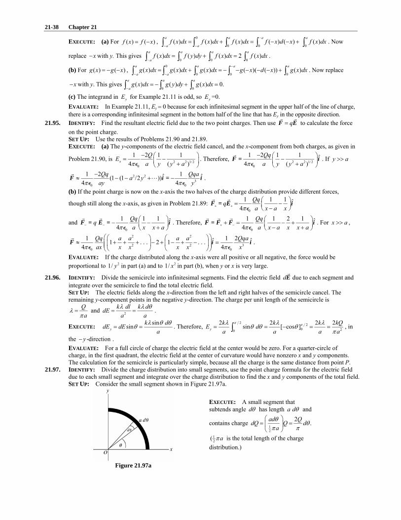
21-38 Chapter 21
EXECUTE: (a) For ( ) ( )f x f x= − , 0
0 0( ) ( ) ( ) ( ) ( )
a a a
a af x dx f x dx f x dx f x d x
−
− −= + = − − +∫ ∫ ∫ ∫ 0
( )a
f x dx∫ . Now
replace x− with y. This gives 0 0 0
( ) ( ) ( ) 2 ( )a a a a
af x dx f y dy f x dx f x dx
−= + =∫ ∫ ∫ ∫ .
(b) For ( ) ( )g x g x= − − , 0
0 0 0( ) ( ) ( ) ( )( ( )) ( )
a a a a
a ag x dx g x dx g x dx g x d x g x dx
−
− −= + = − − − − − +∫ ∫ ∫ ∫ ∫ . Now replace
x− with y. This gives0 0
( ) ( ) ( ) 0.a a a
ag x dx g y dy g x dx
−= − + =∫ ∫ ∫
(c) The integrand in yE for Example 21.11 is odd, so yE =0. EVALUATE: In Example 21.11, Ey 0= because for each infinitesimal segment in the upper half of the line of charge, there is a corresponding infinitesimal segment in the bottom half of the line that has Ey in the opposite direction.
21.95. IDENTIFY: Find the resultant electric field due to the two point charges. Then use q=F E to calculate the force on the point charge. SET UP: Use the results of Problems 21.90 and 21.89. EXECUTE: (a) The y-components of the electric field cancel, and the x-component from both charges, as given in
Problem 21.90, is 2 2 1/ 20
1 2 1 14 ( )x
QEa y y aπ
− ⎛ ⎞= −⎜ ⎟+⎝ ⎠P. Therefore, 2 2 1/ 2
0
1 2 1 1 ˆ4 ( )
Qqa y y aπ
− ⎛ ⎞−⎜ ⎟+⎝ ⎠F = i
P. If y a>>
2 23
0 0
1 2 1ˆ ˆ(1 (1 /2 ))4 4
Qq Qqaa yay yπ π
−≈ − − + ⋅⋅ ⋅ −F i = i
P P.
(b) If the point charge is now on the x-axis the two halves of the charge distribution provide different forces,
though still along the x-axis, as given in Problem 21.89: 0
1 1 1 ˆ4
Qqqa x a xπ+ +⎛ ⎞= −⎜ ⎟−⎝ ⎠
F = E iP
and0
1 1 1 ˆ4
Qqqa x x aπ− −⎛ ⎞− −⎜ ⎟+⎝ ⎠
F = E = iP
. Therefore, 0
1 1 2 1 ˆ4
Qqa x a x x aπ+ −⎛ ⎞+ = − +⎜ ⎟− +⎝ ⎠
F = F F iP
. For x a>> ,
2 2
2 2 30 0
1 1 2ˆ ˆ1 . . . 2 1 . . .4 4
Qq a a a a Qqaax x x x x xπ π
⎛ ⎞⎛ ⎞ ⎛ ⎞≈ + + + − + − + − =⎜ ⎟⎜ ⎟ ⎜ ⎟⎜ ⎟⎝ ⎠ ⎝ ⎠⎝ ⎠
F i iP P
.
EVALUATE: If the charge distributed along the x-axis were all positive or all negative, the force would be proportional to 21/ y in part (a) and to 21/ x in part (b), when y or x is very large.
21.96. IDENTIFY: Divide the semicircle into infinitesimal segments. Find the electric field dE due to each segment and integrate over the semicircle to find the total electric field. SET UP: The electric fields along the x-direction from the left and right halves of the semicircle cancel. The remaining y-component points in the negative y-direction. The charge per unit length of the semicircle is
Qa
λπ
= and 2
k dl k ddEa aλ λ θ
= = .
EXECUTE: sinsinyk ddE dE
aλ θ θθ= = . Therefore,
2 20 20
2 2 2 2sin [ cos ]yk k k kQE da a a a
π πλ λ λθ θ θπ
= = − = =∫ , in
the -directiony− . EVALUATE: For a full circle of charge the electric field at the center would be zero. For a quarter-circle of charge, in the first quadrant, the electric field at the center of curvature would have nonzero x and y components. The calculation for the semicircle is particularly simple, because all the charge is the same distance from point P.
21.97. IDENTIFY: Divide the charge distribution into small segments, use the point charge formula for the electric field due to each small segment and integrate over the charge distribution to find the x and y components of the total field. SET UP: Consider the small segment shown in Figure 21.97a.
EXECUTE: A small segment that subtends angle dθ has length a dθ and
contains charge 12
2 .ad QdQ Q daθ θπ π
⎛ ⎞= =⎜ ⎟⎝ ⎠
12( aπ is the total length of the charge
distribution.)
Figure 21.97a

Electric Charge and Electric Field 21-39
The charge is negative, so the field at the origin is directed toward the small segment. The small segment is located at angle θ as shown in the sketch. The electric field due to dQ is shown in Figure 21.97b, along with its components.
20
14
dQdE
aπ=
P
2 202
QdE da
θπ
=P
Figure 21.97b
( )2 20cos / 2 cosxdE dE Q a dθ π θ θ= = P
( )/ 2 / 202 2 2 2 2 20
0 0 0
cos sin2 2 2x x
Q Q QE dE da a a
π πθ θ θπ π π
= = = =∫ ∫P P P
( )2 20sin / 2 sinydE dE Q a dθ π θ θ= = P
( )/ 2 / 202 2 2 2 2 20
0 0 0
sin cos2 2 2y y
Q Q QE dE da a a
π πθ θ θπ π π
= = = − =∫ ∫P P P
EVALUATE: Note that ,x yE E= as expected from symmetry.
21.98. IDENTIFY: Apply 0xF =∑ and 0yF =∑ to the sphere, with x horizontal and y vertical.
SET UP: The free-body diagram for the sphere is given in Figure 21.98. The electric field E of the sheet is
directed away from the sheet and has magnitude 02
E σ=P
(Eq.21.12).
EXECUTE: 0yF =∑ gives cosT mgα = and cosmgTα
= . 0xF =∑ gives 0
sin2qT σα =P
and 02 sinqT σ
α=P
.
Combining these two equations we have 0cos 2 sin
mg qσα α=P
and 0
tan2
qmgσα =P
. Therefore, 0
arctan2
qmgσα
⎛ ⎞= ⎜ ⎟
⎝ ⎠P.
EVALUATE: The electric field of the sheet, and hence the force it exerts on the sphere, is independent of the distance of the sphere from the sheet.
Figure 21.98
21.99. IDENTIFY: Each wire produces an electric field at P due to a finite wire. These fields add by vector addition.
SET UP: Each field has magnitude 2 2
0
14
Qx x aπ +P
. The field due to the negative wire points to the left, while
the field due to the positive wire points downward, making the two fields perpendicular to each other and of equal
magnitude. The net field is the vector sum of these two, which is Enet = 2E1 cos 45° = 2 2
0
12 cos454
Qx x aπ
°+P
. In
part (b), the electrical force on an electron at P is eE.
EXECUTE: (a) The net field is Enet = 2 2
0
12 cos454
Qx x aπ
°+P
.
Enet = ( )( )9 2 2 6
2 2
2 9.00 10 N m /C 2.50 10 C cos45
(0.600 m) (0.600 m) (0.600 m)
−× ⋅ × °
+ = 6.25 × 10⁴ N/C.
The direction is 225° counterclockwise from an axis pointing to the right through the positive wire.

21-40 Chapter 21
(b) F = eE = (1.60 × 10⁻¹⁹ C)(6.25 × 10⁴ N/C) = 1.00 × 10⁻¹⁴ N, opposite to the direction of the electric field, since the electron has negative charge. EVALUATE: Since the electric fields due to the two wires have equal magnitudes and are perpendicular to each other, we only have to calculate one of them in the solution.
21.100. IDENTIFY: Each sheet produces an electric field that is independent of the distance from the sheet. The net field is the vector sum of the two fields. SET UP: The formula for each field is 0/2 ,E σ= P and the net field is the vector sum of these,
net0 0 02 2 2B A B AE σ σ σ σ±
= ± =P P P
, where we use the + or – sign depending on whether the fields are in the same or
opposite directions and Bσ and Aσ are the magnitudes of the surface charges. EXECUTE: (a) The two fields oppose and the field of B is stronger than that of A, so
Enet = 0 0 02 2 2B A B Aσ σ σ σ−− =
P P P = ( )
2 2
12 2 2
11.6 C/m 9.50 C/m2 8.85 10 C /N m
µ µ−
−× ⋅
= 1.19 × 10⁵ N/C, to the right.
(b) The fields are now in the same direction, so their magnitudes add. Enet = (11.6 µC/m2 + 9.50 µC/m2)/2 0P = 1.19 × 10⁶ N/C, to the right
(c) The fields add but now point to the left, so Enet = 1.19 × 10⁶ N/C, to the left. EVALUATE: We can simplify the calculations by sketching the fields and doing an algebraic solution first.
21.101. IDENTIFY: Each sheet produces an electric field that is independent of the distance from the sheet. The net field is the vector sum of the two fields. SET UP: The formula for each field is 0/ 2 ,E σ= P and the net field is the vector sum of these,
net0 0 02 2 2B A B AE σ σ σ σ±
= ± =P P P
, where we use the + or – sign depending on whether the fields are in the same or
opposite directions and Bσ and Aσ are the magnitudes of the surface charges. EXECUTE: (a) The fields add and point to the left, giving Enet = 1.19 × 10⁶ N/C. (b) The fields oppose and point to the left, so Enet = 1.19 × 10⁵ N/C. (c) The fields oppose but now point to the right, giving Enet = 1.19 × 10⁵ N/C. EVALUATE: We can simplify the calculations by sketching the fields and doing an algebraic solution first.
21.102. IDENTIFY: The sheets produce an electric field in the region between them which is the vector sum of the fields from the two sheets. SET UP: The force on the negative oil droplet must be upward to balance gravity. The net electric field between the sheets is 0/ ,E σ= P and the electrical force on the droplet must balance gravity, so qE = mg. EXECUTE: (a) The electrical force on the drop must be upward, so the field should point downward since the drop is negative. (b) The charge of the drop is 5e, so 0. (5 )( / )qE mg e mgσ= =P and
( )( )( )( )
9 2 12 2 20
19
324 10 kg 9.80 m/s 8.85 10 C /N m5 5 1.60 10 C
mge
σ− −
−
× × ⋅= =
×P = 35.1 C/m2
EVALUATE: Balancing oil droplets between plates was the basis of the Milliken Oil-Drop Experiment which produced the first measurement of the mass of an electron.
21.103. IDENTIFY and SET UP: Example 21.12 gives the electric field due to one infinite sheet. Add the two fields as vectors. EXECUTE: The electric field due to the first sheet, which is in the xy-plane, is ( )1 0
ˆ/ 2 for 0zσ= >E kP and
( )1 0ˆ/2 for 0.zσ= − <E kP We can write this as ( )( )1 0
ˆ/2 / ,z zσ=E kP since / 1 for 0z z z= + > and / / 1z z z z= − = −
for 0.z < Similarly, we can write the electric field due to the second sheet as ( )( )2 0ˆ/2 / ,x xσ= −E iP since its
charge density is .σ− The net field is ( ) ( ) ( )( )1 2 0ˆ ˆ/2 / / .x x z zσ= + = − +E E E i kP
EVALUATE: The electric field is independent of the y-component of the field point since displacement in the -y± direction is parallel to both planes. The field depends on which side of each plane the field is located.
21.104. IDENTIFY: Apply Eq.(21.11) for the electric field of a disk. The hole can be described by adding a disk of charge density σ− and radius 1R to a solid disk of charge density σ+ and radius 2R .
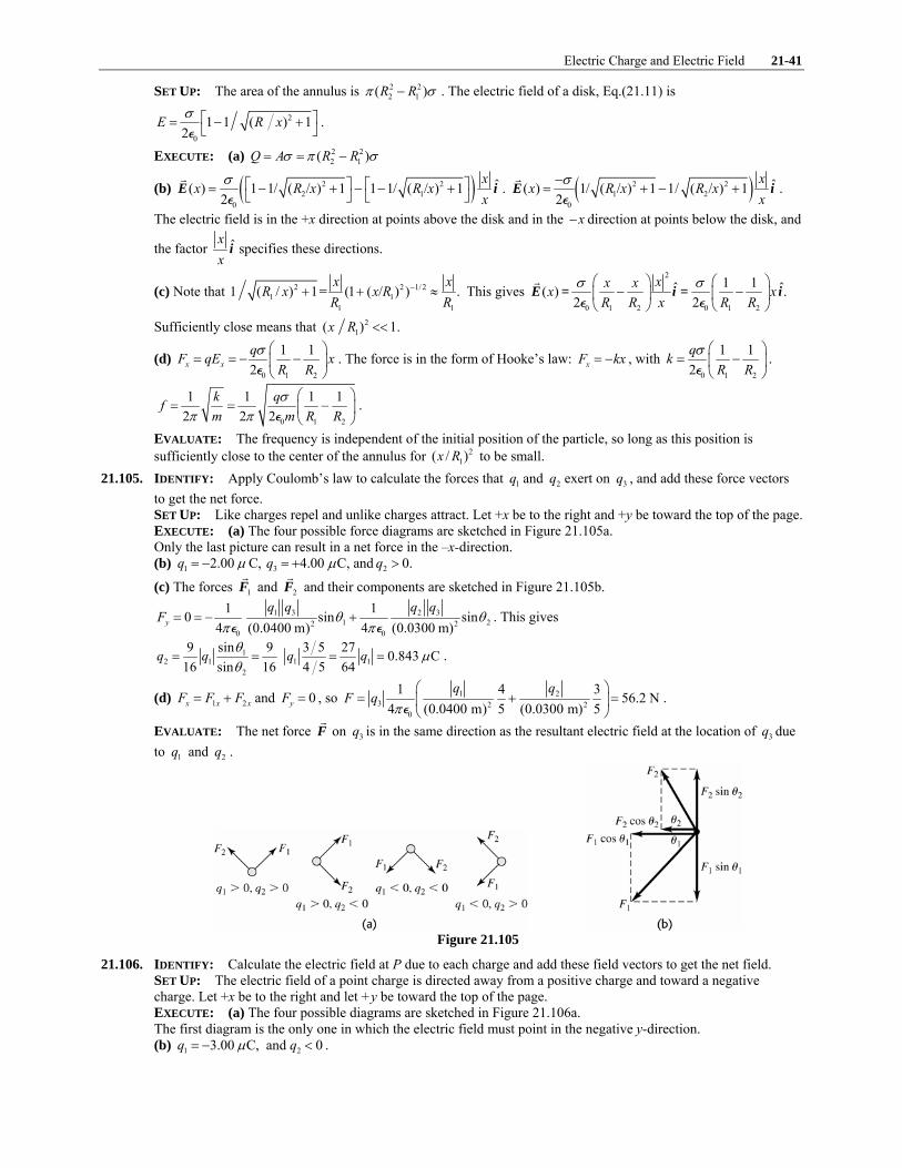
Electric Charge and Electric Field 21-41
SET UP: The area of the annulus is 2 22 1( )R Rπ σ− . The electric field of a disk, Eq.(21.11) is
2
0
1 1 ( ) 12
E R xσ ⎡ ⎤= − +⎣ ⎦P.
EXECUTE: (a) 2 22 1( )Q A R Rσ π σ= = −
(b) ( )2 22 1
0
ˆ( ) 1 1/ ( / ) 1 1 1/ ( / ) 12
xx R x R x
xσ ⎡ ⎤ ⎡ ⎤= − + − − +⎣ ⎦ ⎣ ⎦E iP
. ( )2 21 2
0
ˆ( ) 1/ ( / ) 1 1/ ( / ) 12
xx R x R x
xσ−
= + − +E iP
.
The electric field is in the +x direction at points above the disk and in the x− direction at points below the disk, and
the factor ˆxx
i specifies these directions.
(c) Note that 2 2 1/ 21 1
1 1
1 ( / ) 1= (1 ( / ) ) .x x
R x x RR R
−+ + ≈ This gives 2
0 1 2 0 1 2
1 1ˆ ˆ( ) .2 2
xx xx xR R x R R
σ σ⎛ ⎞ ⎛ ⎞− −⎜ ⎟ ⎜ ⎟
⎝ ⎠ ⎝ ⎠E = i = i
P P
Sufficiently close means that 21( ) 1.x R <<
(d) 0 1 2
1 12x xqF qE x
R Rσ ⎛ ⎞
= = − −⎜ ⎟⎝ ⎠P
. The force is in the form of Hooke’s law: xF kx= − , with 0 1 2
1 12qk
R Rσ ⎛ ⎞
= −⎜ ⎟⎝ ⎠P
.
0 1 2
1 1 1 1 2 2 2
k qfm m R R
σπ π
⎛ ⎞= = −⎜ ⎟
⎝ ⎠P.
EVALUATE: The frequency is independent of the initial position of the particle, so long as this position is sufficiently close to the center of the annulus for 2
1( / )x R to be small. 21.105. IDENTIFY: Apply Coulomb’s law to calculate the forces that 1q and 2q exert on 3q , and add these force vectors
to get the net force. SET UP: Like charges repel and unlike charges attract. Let +x be to the right and +y be toward the top of the page. EXECUTE: (a) The four possible force diagrams are sketched in Figure 21.105a. Only the last picture can result in a net force in the –x-direction. (b) 1 3 22.00 C, 4.00 C, and 0.q q qμ μ= − = + >
(c) The forces 1F and 2F and their components are sketched in Figure 21.105b.
1 3 2 31 22 2
0 0
1 10 sin sin4 (0.0400 m) 4 (0.0300 m)y
q q q qF θ θ
π π= = − +
P P. This gives
12 1 1 1
2
9 sin 9 3 5 27 0.843 C16 sin 16 4 5 64
q q q qθ μθ
= = = = .
(d) 1 2x x xF F F= + and 0yF = , so 1 23 2 2
0
1 4 3 56.2 N4 (0.0400 m) 5 (0.0300 m) 5
q qF q
π⎛ ⎞
= + =⎜ ⎟⎝ ⎠P
.
EVALUATE: The net force F on 3q is in the same direction as the resultant electric field at the location of 3q due to 1q and 2q .
Figure 21.105
21.106. IDENTIFY: Calculate the electric field at P due to each charge and add these field vectors to get the net field. SET UP: The electric field of a point charge is directed away from a positive charge and toward a negative charge. Let +x be to the right and let +y be toward the top of the page. EXECUTE: (a) The four possible diagrams are sketched in Figure 21.106a. The first diagram is the only one in which the electric field must point in the negative y-direction. (b) 1 23.00 C, and 0q qμ= − < .

21-42 Chapter 21
(c) The electric fields 1E and 2E and their components are sketched in Figure 24.106b. 15cos
13θ = , 1
12sin13
θ = ,
212cos13
θ = and 25sin
13θ = . 1 2
2 2
5 120(0.050 m) 13 (0.120 m) 13x
k q k qE = = − + . This gives 2 1
2 2
5(0.120 m) (0.050 m) 12
k q k q= .
Solving for 2q gives 2 7.2 μCq = , so 2 7.2 μCq = − . Then
1 722 2
12 5 1.17 10 N/C(0.050 m) 13 (0.120 m) 13y
k q kqE = − − = − × . 71.17 10 N/CE = × .
EVALUATE: With 1q known, specifying the direction of E determines both 2q and E.
Figure 21.106
21.107. IDENTIFY: To find the electric field due to the second rod, divide that rod into infinitesimal segments of length dx, calculate the field dE due to each segment and integrate over the length of the rod to find the total field due to the rod. Use d dq=F E to find the force the electric field of the second rod exerts on each infinitesimal segment of the first rod. SET UP: An infinitesimal segment of the second rod is sketched in Figure 21.107. ( / )dQ Q L dx′= .
EXECUTE: (a) 2 2
( / 2 ) ( / 2 )
k dQ kQ dxdEx a L x L x a L x
′= =
′ ′+ + − + + −.
20 00
1 1 1( / 2 ) / 2 / 2 / 2
LL L
x xkQ dx kQ kQE dEL x a L x L x a L x L x a x a L
′ ⎡ ⎤ ⎛ ⎞= = = = −⎜ ⎟⎢ ⎥′ ′+ + − + + − + + +⎣ ⎦ ⎝ ⎠∫ ∫ .
2 1 12 2 2x
kQEL x a L x a
⎛ ⎞= −⎜ ⎟+ + +⎝ ⎠.
(b) Now consider the force that the field of the second rod exerts on an infinitesimal segment dq of the first rod. This force is in the +x-direction. dF dq E= .
22 2
22 2
2 1 12 2 2
L a L a
a a
EQ kQF E dq dx dxL L x a L x a
+ + ⎛ ⎞= = = −⎜ ⎟+ + +⎝ ⎠∫ ∫ ∫ .
( )2 2
2 22 22 2
2 1 2 2 2[ln ( 2 )] [ln(2 2 )] 1n2 2 4 2
L a L aa a
kQ kQ a L a L aF a x L x aL L a L a
+ + ⎛ + + + ⎞⎛ ⎞ ⎛ ⎞= + − + + = ⎜ ⎟⎜ ⎟ ⎜ ⎟+⎝ ⎠ ⎝ ⎠⎝ ⎠.
2 2
2
( )1n( 2 )
kQ a LFL a a L
⎛ ⎞+= ⎜ ⎟+⎝ ⎠
.
(c) For a L>> , 2 2 2 2
2 2 2
(1 )1n (21n (1 ) ln(1 2 ))(1 2 )
kQ a L a kQF L a L aL a L a L
⎛ ⎞+= = + − +⎜ ⎟+⎝ ⎠
.
For small z, 2
ln(1 )2zz z+ ≈ − . Therefore, for a L>> ,
2 2 2 2
2 2 2 2
2 222
kQ L L L L kQFL a a a a a
⎛ ⎞⎛ ⎞ ⎛ ⎞≈ − + ⋅ ⋅ ⋅ − − + ⋅ ⋅ ⋅ ≈⎜ ⎟⎜ ⎟ ⎜ ⎟⎜ ⎟⎝ ⎠ ⎝ ⎠⎝ ⎠
.
EVALUATE: The distance between adjacent ends of the rods is a. When a L>> the distance between the rods is much greater than their lengths and they interact as point charges.
Figure 21.107