e cient computation of sparse matrix functions for large...
TRANSCRIPT

Efficient computation of sparse matrix
functions for large scale electronic
structure calculations: The CheSS
library
Stephan Mohr, William Dawson, Michael Wagner, Damien
Caliste, Takahito Nakajima, Luigi Genovese
Barcelona Supercomputing Center
MaX Conference
Trieste, 30th January 2018
Motivation and Applicability Theory Sparsity Accuracy and scaling Parallel scaling Comparison Outlook
Outline
1 Motivation and Applicability
2 Theory behind CheSS
3 Sparsity and truncation
4 Accuracy and scaling with matrix properties
5 Parallel scaling
6 Comparison with other methods
7 Outlook and conclusions
2 / 20
Motivation and Applicability Theory Sparsity Accuracy and scaling Parallel scaling Comparison Outlook
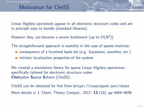
Motivation for CheSS
Linear Algebra operations appear in all electronic structure codes and arein principle easy to handle (standard libraries).
However they can become a severe bottleneck (up to O(N3)).
The straightforward approach is wasteful in the case of sparse matrices:
consequence of a localized basis set (e.g. Gaussians, wavelets, etc.)
intrinsic localization properties of the system
We created a standalone library for sparse Linear Algebra operations,specifically tailored for electronic structure codes:Chebyshev Sparse Solvers (CheSS).
CheSS can be obtained for free from https://launchpad.net/chess
More details in J. Chem. Theory Comput., 2017, 13 (10), pp 4684–4698
3 / 20
Motivation and Applicability Theory Sparsity Accuracy and scaling Parallel scaling Comparison Outlook
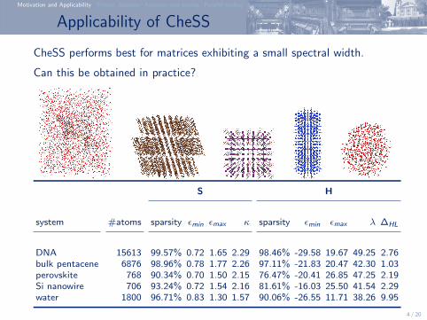
Applicability of CheSS
CheSS performs best for matrices exhibiting a small spectral width.
Can this be obtained in practice?
S H
system #atoms sparsity εmin εmax κ sparsity εmin εmax λ ∆HL
DNA 15613 99.57% 0.72 1.65 2.29 98.46% -29.58 19.67 49.25 2.76bulk pentacene 6876 98.96% 0.78 1.77 2.26 97.11% -21.83 20.47 42.30 1.03perovskite 768 90.34% 0.70 1.50 2.15 76.47% -20.41 26.85 47.25 2.19Si nanowire 706 93.24% 0.72 1.54 2.16 81.61% -16.03 25.50 41.54 2.29water 1800 96.71% 0.83 1.30 1.57 90.06% -26.55 11.71 38.26 9.95
4 / 20
Motivation and Applicability Theory Sparsity Accuracy and scaling Parallel scaling Comparison Outlook
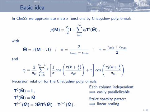
Basic idea
In CheSS we approximate matrix functions by Chebyshev polynomials:
p(M) =c0
2I +
npl∑i=1
ciTi (M̃) ,
with
M̃ = σ(M− τ I) ; σ =2
εmax − εmin; τ =
εmin + εmax
2
and
cj =2
npl
npl−1∑k=0
f
[1
σcos
(π(k + 1
2 )
npl
)+ τ
]cos
(πj(k + 1
2
npl
).
Recursion relation for the Chebyshev polynomials:
T0(M̃) = I ,
T1(M̃) = M̃ ,
Tj+1(M̃) = 2M̃Tj(M̃)− Tj−1(M̃) .
Each column independent=⇒ easily parallelizable
Strict sparsity pattern=⇒ linear scaling
5 / 20

Motivation and Applicability Theory Sparsity Accuracy and scaling Parallel scaling Comparison Outlook
Available functions
CheSS can calculate those matrix functions needed for DFT:
density matrix: f (x) = 11+eβ(x−µ)
(or f (x) = 12
[1− erf
(β(ε− x)
)])
energy density matrix: f (x) = x1+eβ(x−µ)
(or f (x) = x2
[1− erf
(β(ε− x)
)])
matrix powers: f (x) = xa (a can be non-integer!)
We can calculate arbitrary functions by changing only the coefficients cj !
Only requirement:function f must be well representable by Chebyshev polynomials over theentire eigenvalue spectrum.
6 / 20
Motivation and Applicability Theory Sparsity Accuracy and scaling Parallel scaling Comparison Outlook
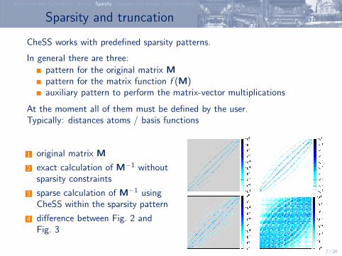
Sparsity and truncation
CheSS works with predefined sparsity patterns.
In general there are three:pattern for the original matrix Mpattern for the matrix function f (M)auxiliary pattern to perform the matrix-vector multiplications
At the moment all of them must be defined by the user.Typically: distances atoms / basis functions
1 original matrix M
2 exact calculation of M−1 withoutsparsity constraints
3 sparse calculation of M−1 usingCheSS within the sparsity pattern
4 difference between Fig. 2 andFig. 3
7 / 20
Motivation and Applicability Theory Sparsity Accuracy and scaling Parallel scaling Comparison Outlook
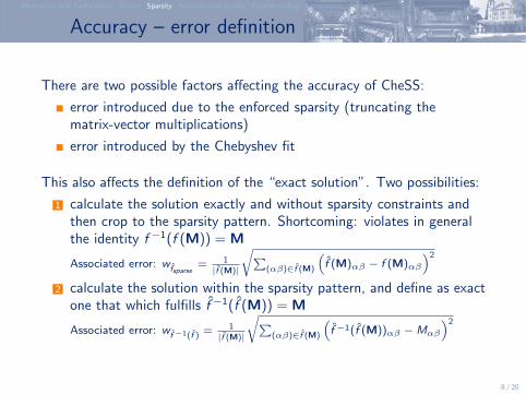
Accuracy – error definition
There are two possible factors affecting the accuracy of CheSS:
error introduced due to the enforced sparsity (truncating thematrix-vector multiplications)
error introduced by the Chebyshev fit
This also affects the definition of the “exact solution”. Two possibilities:
1 calculate the solution exactly and without sparsity constraints andthen crop to the sparsity pattern. Shortcoming: violates in generalthe identity f −1(f (M)) = M
Associated error: wf̂sparse= 1|f̂ (M)|
√∑(αβ)∈f̂ (M)
(f̂ (M)αβ − f (M)αβ
)2
2 calculate the solution within the sparsity pattern, and define as exactone that which fulfills f̂ −1(f̂ (M)) = M
Associated error: wf̂−1(f̂ ) = 1|f̂ (M)|
√∑(αβ)∈f̂ (M)
(f̂ −1(f̂ (M))αβ −Mαβ
)2
8 / 20

Motivation and Applicability Theory Sparsity Accuracy and scaling Parallel scaling Comparison Outlook
Fixed versus variable sparsity
Alternative to a fixed sparsity pattern: Variable adaption during theiterations (e.g. based on the magnitude of the entries).
Advantage: Flexible control of the truncation error
Shortcoming: The sparsity may decrease considerably
Example: Purification method (TRS4 by Niklasson)
Sparsity defined by magnitude
Strong fill-in during the iterations
Cost of matrix multiplicationsincreases
Unlike CheSS the matrix to beapplied changes ⇒ harder toparallelize 92
93
94
95
96
97
98
99
2 4 6 8 10 12 14 16
sp
ars
ity in
%
iteration
sparsity
9 / 20
Motivation and Applicability Theory Sparsity Accuracy and scaling Parallel scaling Comparison Outlook
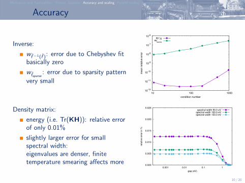
Accuracy
Inverse:
wf̂ −1(f̂ ): error due to Chebyshev fitbasically zero
wf̂sparse: error due to sparsity pattern
very small
10-12
10-11
10-10
10-9
10-8
10-7
10-6
10 100 1000
mean r
ela
tive e
rror
condition number
wf̂-1
(f̂)wf̂sparse
Density matrix:
energy (i.e. Tr(KH)): relative errorof only 0.01%
slightly larger error for smallspectral width:eigenvalues are denser, finitetemperature smearing affects more
0.000
0.005
0.010
0.015
0.020
0.025
0.001 0.01 0.1 1
rela
tive
err
or
in %
gap (eV)
spectral width 50.0 eVspectral width 100.0 eVspectral width 150.0 eV
10 / 20
Motivation and Applicability Theory Sparsity Accuracy and scaling Parallel scaling Comparison Outlook
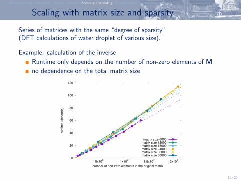
Scaling with matrix size and sparsity
Series of matrices with the same “degree of sparsity”(DFT calculations of water droplet of various size).
Example: calculation of the inverse
Runtime only depends on the number of non-zero elements of M
no dependence on the total matrix size
0
20
40
60
80
100
120
5x10⁶
1x10⁷
1.5x10⁷
2x10⁷
run
tim
e (
se
co
nd
s)
number of non-zero elements in the original matrix
matrix size 6000matrix size 12000matrix size 18000matrix size 24000matrix size 30000matrix size 36000
11 / 20
Motivation and Applicability Theory Sparsity Accuracy and scaling Parallel scaling Comparison Outlook
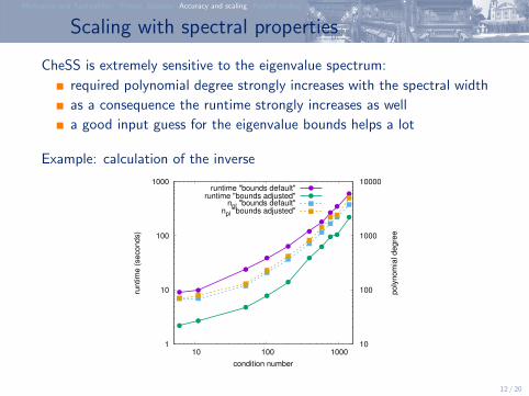
Scaling with spectral properties
CheSS is extremely sensitive to the eigenvalue spectrum:
required polynomial degree strongly increases with the spectral width
as a consequence the runtime strongly increases as well
a good input guess for the eigenvalue bounds helps a lot
Example: calculation of the inverse
1
10
100
1000
10 100 1000 10
100
1000
10000
runtim
e (
seconds)
poly
nom
ial degre
e
condition number
runtime "bounds default"runtime "bounds adjusted"
npl "bounds default"npl "bounds adjusted"
12 / 20
Motivation and Applicability Theory Sparsity Accuracy and scaling Parallel scaling Comparison Outlook
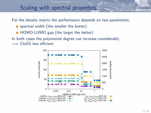
Scaling with spectral properties
For the density matrix the performance depends on two parameters:
spectral width (the smaller the better)
HOMO-LUMO gap (the larger the better)
In both cases the polynomial degree can increase considerably=⇒ CheSS less efficient.
0
50
100
150
200
0.001 0.01 0.1 1 0
500
1000
1500
2000
2500
3000
run
tim
e (
se
co
nd
s)
po
lyn
om
ial d
eg
ree
HOMO-LUMO gap (eV)runtime, εmax-εmin=50.0 eV
runtime, εmax-εmin=100.0 eVruntime, εmax-εmin=150.0 eV
npl, εmax-εmin=50.0 eVnpl, εmax-εmin=100.0 eVnpl, εmax-εmin=150.0 eV
13 / 20
Motivation and Applicability Theory Sparsity Accuracy and scaling Parallel scaling Comparison Outlook
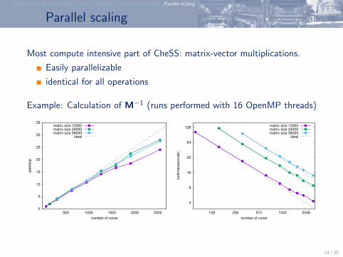
Parallel scaling
Most compute intensive part of CheSS: matrix-vector multiplications.
Easily parallelizable
identical for all operations
Example: Calculation of M−1 (runs performed with 16 OpenMP threads)
0
5
10
15
20
25
30
35
500 1000 1500 2000 2500
sp
ee
du
p
number of cores
matrix size 12000matrix size 24000matrix size 36000
ideal
4
8
16
32
64
128
128 256 512 1024 2048
run
tim
e(s
eco
nd
s)
number of cores
matrix size 12000matrix size 24000matrix size 36000
ideal
14 / 20

Motivation and Applicability Theory Sparsity Accuracy and scaling Parallel scaling Comparison Outlook
Extreme scaling
We have also performed extreme-scaling tests from 1536 to 16384 cores.
Example: Calculation of M−1 (runs performed with 8 OpenMP threads)
1
2
3
4
5
6
7
8
9
10
11
2000 4000 6000 8000 10000 12000 14000 16000
speedup
number of cores
matrix size 96000ideal
Given the small matrix (96000× 96000) the obtained scaling is good.
We will try to further improve the scaling.15 / 20
Motivation and Applicability Theory Sparsity Accuracy and scaling Parallel scaling Comparison Outlook
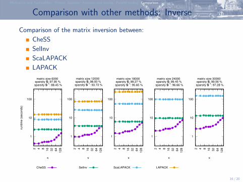
Comparison with other methods: Inverse
Comparison of the matrix inversion between:
CheSS
SelInv
ScaLAPACK
LAPACK
1
10
100
2 4 8
16
32
64
128
runtim
e (
seconds)
κ
matrix size 6000 sparsity S: 97.95 % sparsity S
-1: 88.45 %
CheSS
1
10
100
2 4 8
16
32
64
128
κ
matrix size 12000 sparsity S: 98.93 % sparsity S
-1: 93.73 %
SelInv
1
10
100
2 4 8
16
32
64
128
κ
matrix size 18000 sparsity S: 99.27 % sparsity S
-1: 95.65 %
ScaLAPACK
1
10
100
2 4 8
16
32
64
128
κ
matrix size 24000 sparsity S: 99.45 % sparsity S
-1: 96.66 %
LAPACK
1
10
100
2 4 8
16
32
64
128
κ
matrix size 30000 sparsity S: 99.56 % sparsity S
-1: 97.28 %
16 / 20
Motivation and Applicability Theory Sparsity Accuracy and scaling Parallel scaling Comparison Outlook
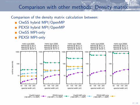
Comparison with other methods: Density matrix
Comparison of the density matrix calculation between:
CheSS hybrid MPI/OpenMP
PEXSI hybrid MPI/OpenMP
CheSS MPI-only
PEXSI MPI-only
10
100
1000
50 100 150 200
runtim
e (
seconds)
spectral width (eV)
matrix size 6000 sparsity S: 97.95 % sparsity H: 92.97 % sparsity K: 88.45 %
CheSS hybrid(160 MPI x 12 OMP)
10
100
1000
50 100 150 200
spectral width (eV)
matrix size 12000 sparsity S: 98.93 % sparsity H: 96.25 % sparsity K: 93.73 %
PEXSI hybrid(160 MPI x 12 OMP)
10
100
1000
50 100 150 200
spectral width (eV)
matrix size 18000 sparsity S: 99.27 % sparsity H: 97.42 % sparsity K: 95.65 %
CheSS MPI-only(1920 MPI x 1 OMP)
10
100
1000
50 100 150 200
spectral width (eV)
matrix size 24000 sparsity S: 99.27 % sparsity H: 97.42 % sparsity K: 95.65 %
PEXSI MPI-only(1920 MPI x 1 OMP)
10
100
1000
50 100 150 200
spectral width (eV)
matrix size 30000 sparsity S: 99.27 % sparsity H: 97.42 % sparsity K: 95.65 %
17 / 20
Motivation and Applicability Theory Sparsity Accuracy and scaling Parallel scaling Comparison Outlook
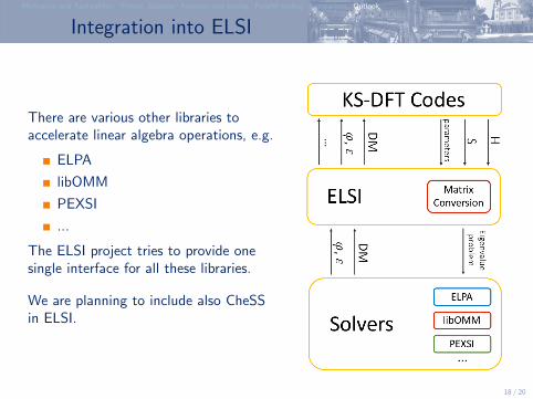
Integration into ELSI
There are various other libraries toaccelerate linear algebra operations, e.g.
ELPA
libOMM
PEXSI
...
The ELSI project tries to provide onesingle interface for all these libraries.
We are planning to include also CheSSin ELSI.
18 / 20
Motivation and Applicability Theory Sparsity Accuracy and scaling Parallel scaling Comparison Outlook
Conclusions
CheSS is a flexible tool to calculate matrix functions for DFT
can easily be extended to other functions
exploits sparsity of the matrices, linear scaling possible
works best for small spectral widths of the matrices
very good parallel scaling (both MPI and OpenMP)
19 / 20