Efficient Lookup on Unstructured Topologies∗

Ruggero Morselli†, Bobby Bhattacharjee†,‡, Michael A. Marsh‡, and Aravind Srinivasan†,‡

Abstract

We present LMS, a protocol for efficient lookup on unstructured networks. Our protocol uses a virtualnamespace without imposing specific topologies. It is more efficient than existing lookup protocols forunstructured networks, and thus is an attractive alternative for applications in which the topology cannotbe structured as a Distributed Hash Table (DHT).

We present analytic bounds for the worst-case performance of our protocol. Through detailed sim-ulations (with up to 100,000 nodes), we show that the actual performance on realistic topologies issignificantly better. We also show in both simulations and a complete implementation (which includesover five hundred nodes) that our protocol is inherently robust against multiple node failures and canadapt its replication strategy to optimize searches according to a specific heuristic. Moreover, the sim-ulation demonstrates the resilience of LMS to high node turnover rates, and that it can easily adapt toorders of magnitude changes in network size. The overhead incurred by LMS is small, and its performanceapproaches that of DHTs on networks of similar size.

1 Introduction

Large peer-to-peer networks require efficient object lookup mechanisms. Flooding searches, while adequatefor small networks, quickly become untenable as networks grow larger. Consequently, research has progressedalong two avenues: more efficient lookup protocols that operate on general (unstructured) topologies, andfundamentally new lookup strategies that achieve bounded worst-case performance by adding constraints tothe network topology. The latter, while very efficient, might not be usable when the peer-to-peer applicationplaces its own constraints on the topology. This is especially the case when the links in the topology haveparticular significance, such as expressing statements of trust or belief between peers. From an algorithmicperspective, this sort of network topology appears to be unstructured.

We approach this issue by considering a model where a graph G is given (the topology), such that eachpeer in the system corresponds to a vertex u of G and can only send messages to peers that correspond toneighbors of u in G. Developing distributed protocols in this model is not only an interesting theoreticalproblem, but has several practical applications, such as that outlined in Section 6. In this paper, wepresent the Local Minima Search (LMS) protocol for unstructured topologies. LMS extends the notion ofrandom walks, which to date have proved the most promising approach to improving search performanceon unstructured networks [18, 14, 6]. In addition, LMS borrows the ideas of namespace virtualization andconsistent hashing employed by constrained-topology protocols such as distributed hash tables (DHTs) [29,33, 31, 19]. Namespace virtualization maps both peers and objects to identifiers in a single large space.

In LMS, the owner of each object places replicas of the object on several nodes. Like in a DHT, LMSplaces replicas onto nodes which have IDs “close” to the object. Unlike in a DHT, however, in an unstructuredtopology there is no mechanism to route to the node which is the closest to an item. Instead, we introduce

∗Full version. Technical report CS-TR-4772, Department of Computer Science, University of Maryland, December 2005.Obsoletes CS-TR-4593. Also filed as UMIACS-TR-2005-75. An extended abstract of this paper appeared in ACM PODC2005, Las Vegas, NV, July 2005. This material is based upon work supported in part by: NSF grant 0208005, ITR AwardCNS-0426683, NSF grant CCR-0310499, NSF award ANI0092806 and DoD contract MDA90402C0428. We thank past refereesof this work for their valuable comments.

†Department of Computer Science, University of Maryland, College Park, MD 20742.‡Institute for Advanced Computer Studies, University of Maryland, College Park, MD 20742.

1

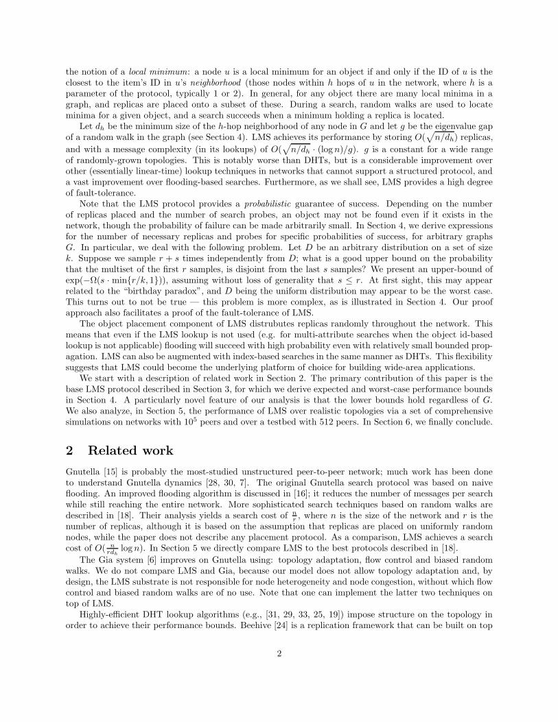
the notion of a local minimum: a node u is a local minimum for an object if and only if the ID of u is theclosest to the item’s ID in u’s neighborhood (those nodes within h hops of u in the network, where h is aparameter of the protocol, typically 1 or 2). In general, for any object there are many local minima in agraph, and replicas are placed onto a subset of these. During a search, random walks are used to locateminima for a given object, and a search succeeds when a minimum holding a replica is located.

Let dh be the minimum size of the h-hop neighborhood of any node in G and let g be the eigenvalue gapof a random walk in the graph (see Section 4). LMS achieves its performance by storing O(

√

n/dh) replicas,

and with a message complexity (in its lookups) of O(√

n/dh · (log n)/g). g is a constant for a wide rangeof randomly-grown topologies. This is notably worse than DHTs, but is a considerable improvement overother (essentially linear-time) lookup techniques in networks that cannot support a structured protocol, anda vast improvement over flooding-based searches. Furthermore, as we shall see, LMS provides a high degreeof fault-tolerance.

Note that the LMS protocol provides a probabilistic guarantee of success. Depending on the numberof replicas placed and the number of search probes, an object may not be found even if it exists in thenetwork, though the probability of failure can be made arbitrarily small. In Section 4, we derive expressionsfor the number of necessary replicas and probes for specific probabilities of success, for arbitrary graphsG. In particular, we deal with the following problem. Let D be an arbitrary distribution on a set of sizek. Suppose we sample r + s times independently from D; what is a good upper bound on the probabilitythat the multiset of the first r samples, is disjoint from the last s samples? We present an upper-bound ofexp(−Ω(s · minr/k, 1)), assuming without loss of generality that s ≤ r. At first sight, this may appearrelated to the “birthday paradox”, and D being the uniform distribution may appear to be the worst case.This turns out to not be true — this problem is more complex, as is illustrated in Section 4. Our proofapproach also facilitates a proof of the fault-tolerance of LMS.

The object placement component of LMS distrubutes replicas randomly throughout the network. Thismeans that even if the LMS lookup is not used (e.g. for multi-attribute searches when the object id-basedlookup is not applicable) flooding will succeed with high probability even with relatively small bounded prop-agation. LMS can also be augmented with index-based searches in the same manner as DHTs. This flexibilitysuggests that LMS could become the underlying platform of choice for building wide-area applications.

We start with a description of related work in Section 2. The primary contribution of this paper is thebase LMS protocol described in Section 3, for which we derive expected and worst-case performance boundsin Section 4. A particularly novel feature of our analysis is that the lower bounds hold regardless of G.We also analyze, in Section 5, the performance of LMS over realistic topologies via a set of comprehensivesimulations on networks with 105 peers and over a testbed with 512 peers. In Section 6, we finally conclude.

2 Related work

Gnutella [15] is probably the most-studied unstructured peer-to-peer network; much work has been doneto understand Gnutella dynamics [28, 30, 7]. The original Gnutella search protocol was based on naiveflooding. An improved flooding algorithm is discussed in [16]; it reduces the number of messages per searchwhile still reaching the entire network. More sophisticated search techniques based on random walks aredescribed in [18]. Their analysis yields a search cost of n

r , where n is the size of the network and r is thenumber of replicas, although it is based on the assumption that replicas are placed on uniformly randomnodes, while the paper does not describe any placement protocol. As a comparison, LMS achieves a searchcost of O( n

rdhlog n). In Section 5 we directly compare LMS to the best protocols described in [18].

The Gia system [6] improves on Gnutella using: topology adaptation, flow control and biased randomwalks. We do not compare LMS and Gia, because our model does not allow topology adaptation and, bydesign, the LMS substrate is not responsible for node heterogeneity and node congestion, without which flowcontrol and biased random walks are of no use. Note that one can implement the latter two techniques ontop of LMS.

Highly-efficient DHT lookup algorithms (e.g., [31, 29, 33, 25, 19]) impose structure on the topology inorder to achieve their performance bounds. Beehive [24] is a replication framework that can be built on top

2

2

8

1799

32

42

90

9112

63

3528

14

70

45

3basinsfor localminima

localminimum

(a) 1-hop Neighborhoods

2

8

1799

32

42

90

9112

63

3528

14

70

45

3

(b) 2-hop Neighborhoods

Figure 1: Local minima, basins and deterministic forwarding. Nodes are labelled with their distances fromthe key. Concentric circles denote local minima, and shaded regions their basins. Arrows indicate the pathfrom a node towards its local minimum. (a) All forwarding arrows for h = 1. (b) Forwarding arrows fortwo nodes with h = 2. A dashed arrow indicates the target towards which a node forwards a probe whendifferent than the next hop.

of a DHT. These systems employ the same namespace virtualization of which we make use. A virtualizednamespace has previously been used on an unstructured topology in Freenet [8], though for a different reason.

In [2] the authors build a P2P system where publishing involves storing on s random nodes in the graphand searching involves querying s independently chosen random nodes. Unlike LMS, [2] requires that thenodes may modify the topology of the neighborhood graph. The authors prove a result that is similar toTheorem 4.1(i) in this paper, although with a different technique; we thank a referee for bringing this resultto our attention. Other differences are: (a) LMS restricts replica placement to local minima, which improvesefficiency significantly; (b) our Theorem 4.1 is generalized beyond the special case in [2]; and (c) our prooftechnique for Theorem 4.1 also helps us show that LMS is robust under the loss of some replicas.

YAPPERS [12] is a P2P system that, like LMS, assumes a “given topology” model and combines struc-tured and unstructured designs. In YAPPERS, nodes publish an item by storing it at a node of the 2-hopneighborhood, which is structured as a small DHT. Search is achieved by flooding all and only the nodes inthe network that might have the item, and requires nodes to keep state for an extended local neighborhood(within 5 hops). The authors do not present a formal analysis.

Related to the problem of lookup in a given topology is the work on name-independent routing (NIR)in a graph [4, 1, 3]. NIR allows a node to send a message to any other node, in a given topology setting.Existing work on NIR assumes that the topology graph never changes and requires an initial setup phaseperformed by a centralized algorithms that knows the entire graph.

Bloom filters [5, 21], compact digests of sets of elements, have previously been considered for structuredtopologies [26] as a way to provide fast lookup. In this paper, we present an application of Bloom filters ona completely unstructured topology. Theoretical properties of random walks have been exploited by [14] toimprove search in unstructured networks.

3 LMS protocol description

We assume a system of principals (nodes or peers) structured as an overlay network on top of a commu-nications infrastructure such as the Internet. The topology of this overlay network is dictated by externalrequirements, and its maintenance is beyond the scope of our protocol. We assume that nodes can commu-

3

nicate with one another if and only if they are neighbors in the overlay topology.1

Nodes in the system have unique identifiers generated uniformly at random from an ID space of all bitstrings of some length λ. λ must be chosen large enough to guarantee uniqueness with high probability (forexample, 160 bits). How this identifier is constructed is in general application-specific.2

We define a node v’s neighborhood as the set of nodes at most h hops away from v in the overlay. Foreach of these nodes, v knows its unique identifier, how many hops away it is, and v’s next hop towards it.We do not present a protocol for propagating this information, but it is easily implemented by repeatedexchanges of a node’s known h − 1-hop neighborhood. Note that nodes have no knowledge of the topologybeyond this neighborhood.

3.1 Protocol overview

LMS enables nodes to publish data items (i.e. files, documents) and to retrieve data items published byothers. Items published by the system are given key identifiers (or simply keys) in the same ID space as thenodes, for example by hashing the name or contents of the item. The protocol then attempts to store anitem at nodes that are close to its key in the (circular) ID space. In terms of the distance between a nodeand key, we do not find the global minimum (as in a distributed hash table), but rather a local minimum.

Publishing an item involves storing replicas of the item at a number of randomly selected local minima;retrieving an item involves querying randomly selected local minima until one is found that holds a replica.Crucially, the distribution of these random selections is typically not the uniform distribution; it is a functionof the underlying topology, and is naturally generated by the distributed algorithms that we employ. Intu-itively, the more replicas are placed, the easier it will be to find one of them. Random minimum selection isaccomplished by performing a random walk through the overlay before actively looking for a local minimum.

3.2 The basic protocol

For clarity of the exposition, we first present a slightly simplified version of the LMS protocol. In this version,placing and locating items are essentially identical. We will then refine this to account for the differencesbetween the two operations and to add optimizations.

To select a random local minimum, a node generates a probe message, which has the general form 〈probe,initiator, key, walk length, path〉. A probe moves through the network with a random walk followed by adeterministic walk. The walk length parameter is initialized to some positive value. A node that receives theprobe (including the initiator) first examines this parameter. If it is greater than zero, the probe is in therandom walk phase, and the node forwards it to a randomly selected neighbor3 and decrements the value.If walk length is zero, the probe is forwarded according to the deterministic walk, which is described below.In either case, a node appends itself to path before forwarding the probe so that a local minimum can directits response back to the initiator.4

Deterministic walk Deterministic forwarding is done using a greedy algorithm. A node v receiving aprobe computes the distance between key and every node in its neighborhood including itself. We define thedistance between a key x and a node w as d(x, w) = minx − w mod 2λ, w − x mod 2λ.

Let v′ be the node that minimizes d(key, ·) over the neighborhood of v. If v = v′, then v is the localminimum; it then stores or returns a replica, depending on the type of probe. Otherwise, v determines thenext-hop node towards v′ (from its local knowledge of the topology) and forwards the probe to this node.Recall that we assume v cannot communicate directly with v′ if it is more than one hop away.

1This assumption can be weakened and communications made possible over larger distances in the overlay. This does notsubstantially alter the protocol, other than to allow optimizations that reduce the number of messages exchanged.

2For instance, the SHA-1 hash of a node’s public key.3The distribution for this selection is uniform in our case, but nonuniform choice is also possible. For instance, if the

topology is dictated by trust relations, more highly trusted nodes might be given greater weight in selection. Another possibility,introduced in [6], is to weight the distribution according to resource availability.

4If messages can be exchanged by nodes that are not direct neighbors, then path is not needed, since the local minimum cancommunicate directly with the initiator.

4

221

3

5

53

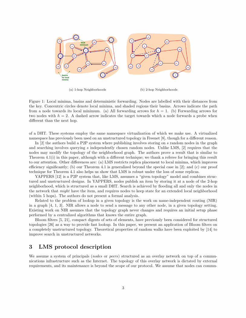
Figure 2: An illustration of “unexpected” message forwarding. Node 5 sees 3 in its 2-hop neighborhood, andforwards the probe to 21, the next hop towards 3. Node 21 sees a better match in 2, and so forwards theprobe to 53 rather than 3.

For a local minimum of a key x, vx, we define the set of nodes that deterministically forward to thisminimum as its basin of attraction (or basin). Note that while it is possible for a local minimum to “attract”nodes from outside of its neighborhood, it is also possible for the basin to be only the minimum itself. Thisis illustrated in Fig. 1. It is also possible that a message “intended” for a node v′ will be redirected towardsa better minimum v′′ at an intermediate hop, as shown in Fig. 2.

3.3 Protocol details

Replica placement We now distinguish between probes for placing replicas and those for locating replicas.A REPLICA-PLACE probe is initiated by the owner of an item, and includes an additional field item. When alocal minimum receives a REPLICA-PLACE probe, it checks if it already holds a replica, and if not whether ithas the resources to store one. If the minimum is able to store a replica of the item, it informs the initiator.

When a local minimum cannot store a new replica, it performs duplication avoidance: doubling theinitial random walk length and restarting the probe’s random walk. Because the probe is starting froma new location, it is less likely to again reach a duplicate minimum than if it were started with the samerandom walk length from the initiator.

We must limit the number of times that duplication avoidance is invoked, because the owner of anitem might attempt to place more replicas than there are local minima for the item’s key. This leads toREPLICA-PLACE probes that circulate through the network indefinitely, with progressively longer randomwalks. Consequently, we include a parameter initialized with the maximum number of failures permitted.Duplication avoidance decrements this parameter, discarding the probe when it becomes negative. The finalform of a REPLICA-PLACE probe is then 〈REPLICA-PLACE, initiator, key, walk length, item, initial walk length,failure count, path〉.

Replica lookup A SEARCH-PROBE performs a lookup operation on an item key. A local minimum thatreceives a SEARCH-PROBE checks whether it holds a replica of the item and returns either the replica or noticeof failure to the initiator. The form of a SEARCH-PROBE is simply 〈SEARCH-PROBE, initiator, key, walk length,path〉.

Note that LMS is a probabilistic algorithm. The probability of a single SEARCH-PROBE locating a replicais fairly low, so a node will have to initiate a number of probes when looking for an item. This can be donein serial or in parallel. The former increases the expected time until the node receives a successful response,while the latter increases the load on the system.

3.4 Variant: Bloom filters

In this section, we describe a variant of the protocol, called the Bloom filter variant, which improves theefficiency of item lookup at the expense of additional communications overhead.

Each node periodically constructs a Bloom filter [5] of the keys for which it holds a replica and providesa copy of this Bloom filter to all the nodes in its hB-neighborhood, where hB is a global parameter. It ispossible for hB to be different than h, the depth of the neighborhood for the definition of local minimum(see Section 3).

5

Use of the filters within LMS is relatively straightforward: upon receiving a SEARCH-PROBE message, anode v can check all of the Bloom filters it holds for each of its hB-hop neighbors. If there is a match of thekey being searched for in the Bloom filter of some neighbor u, v can short-circuit the usual search protocoland forward the SEARCH-PROBE message directly to u.

Note that it is possible to use an attenuated Bloom filter [26] to combine incoming filters and transmitonly a single filter for each distance. Thus, from each neighbor v a node receives a single filter for the itemsreplicated at v, a single filter for all of v’s one hop neighbors, a single filter for v’s two hop neighbors, and soon. It is possible to further reduce the filter overhead by using arithmetic encoding to compress the filters(as described in [21]).

In general, it is not necessary to keep (attenuated) Bloom filters for the entire neighborhood for whicha node keeps ID information (i.e. in general one can choose hB to be smaller than h). Often it is sufficientto choose hB to be 1 or 2 to get significant benefit without incurring the (computation and bandwidth)overhead of constructing and disseminating large filters from multiple hops away.

In the special case that the Bloom filter and identifier neighborhood are identical (i.e., hB = h), thesearch phase of the protocol can dispense with the deterministic walk (Section 3.2). More specifically, ifhB = h, the Bloom filter variant of LMS mandates that search probes only perform a random walk. Thesearch probe fails if walk length reaches 0 without finding a Bloom filter match at any node on the path.We present an analysis of this special case, along with a general analysis of Bloom filters within LMS, inAppendix F.

3.5 The adaptive protocol

Having only local information, a node has no a priori way to know how many replicas of its items it mustplace in order for them to be easily found by other nodes. Increasing the number of replicas reduces theaverage number of search probes needed to find a replica, and vice-versa. Search performance thus providesa feedback mechanism to determine if an item has been replicated sufficiently.

The adaptive protocol is the component of LMS that determines and dynamically adjusts the number ofreplicas to be placed. It is run periodically for each item by its owner and ensures that a sufficient numberr of replicas are available at any time. Let s be the average number of probes needed to find the item at agiven time. The adaptive protocol ensures that s ≈ f(r), where f is an arbitrary function, chosen by theowner.5 For simplicity of the exposition we present the protocol for the case f(r) = r (see Section 4). Theoverhead of this protocol is minimal, aside from any additional replica placements, as it leverages existingactions.

A search from a random node in the system takes on average s probes to find a replica of an item Iowned by node v. Node v periodically learns an estimate of s, as explained below; from the current numberof reachable replicas r, it computes the number of replicas r′ that it adaptively determines are needed asr′ = dαr + (1 − α)se. Here α is a hysteresis parameter between 0 and 1 (we use 0.9) that controls howsensitive the algorithm is to fluctuations in s. We define δ = r′ − r as the needed change in number ofreplicas, and a non-zero value results in either placing or deleting replicas.

Since searches are a normal and frequent part of the system’s operation, it is a simple matter for a node vi

to keep track of the number of probes si it needed to send before finding a replica of I .6 If si is included in aSEARCH-PROBE message, the replica holder can store it and forward a batch of probe results to v periodically.These results provide a representative sample from which v can estimate the average s. Note that nodes onthe threshold of being able to find replicas of I will tend to drive r up, allowing new nodes to find replicasand improving the sampling over the network.

5For example, this could be used to take the popularity of an item into account by storing many more replicas so that mostsearches require very few probes.

6For an unpopular item, the owner of an item might select random nodes and request that they perform searches for theitem to make up for the lack of search feedback.

6

4 Analysis of LMS

We now give a rigorous analysis of the protocol; we make no assumptions about the topology layer, otherthan the necessary condition that the topology, which is a graph G, is connected. The four main resultsderived are: (a) tight bounds on the probability that a search in LMS fails; (b) bounds on the expectedwalk-length (i.e. the number of nodes visited by a search probe, Section 3.2) conditional on successful search;(c) the asymptotic performance of LMS; and (d) robustness under failures.

In Appendix F, we briefly analyze a variant of the protocol that includes Bloom filters.

4.1 Mixing time and eigenvalue gap

We first define the mixing time of a graph and the eigenvalue gap of the random walk. We will use theseconcepts to analyze the performance of LMS.

Let G be a connected directed graph and let n denote the number of nodes in G. Let RW(u, t) be thedistribution of the vertex visited by a random walk on graph G after t steps, starting at vertex u. Only forthe purpose of this analysis, we define the random walk in a way that is slightly different than what we did inthe protocol description (Section 3.2): at each step, the walk remains at the current vertex with probability1/2 and otherwise moves to a uniformly random neighbor. Let P be the probability transition matrix of therandom walk. Namely, P [i, j] (1 ≤ i, j ≤ n) is the probability that the random walk will move from node ito node j, at any step: for all edges (i, j) of G, it is P [i, j] = 1/(2di), where di is the degree of node i; for allnodes i, P [i, i] = 1/2; P [i, j] = 0 otherwise. We denote by 1 = µ1 > µ2 ≥ · · · ≥ µn ≥ 0 the eigenvalues of P .We define the eigenvalue gap of the random walk as g(G) = 1 − µ2.

It is a known fact in graph theory that RW(u, t) approaches a unique stationary distribution SRW , nomatter what the starting vertex u is. SRW places probability d(v)/(2m) on each node v, where d(v) is thedegree —number of neighbors— of v, and m is the total number of edges in G. We want to formalize thisnotion.

We can define the ε-mixing time of G, denoted by T (G, ε), as the smallest integer t such that for anyvertex u it is:

SD(RW(u, t),SRW) ≤ ε/2

where SD(D, D′) = 1

2

∑

i|PrD[i] − PrD′ [i]| denotes the statistical difference between the distributions D and

D′.It is known how to express the ε-mixing time as a function of the eigenvalue gap. To see this, we can

apply a technique analogous to the proof of Theorem 6.21 in [22]: the statistical difference between RW(u, t)and SRW is at most

√n(µ2)

t. From this, we obtain the following expression for the ε-mixing time:

T (G, ε) ≤ 1

g

[

1

2ln n + ln(1/ε)

]

. (1)

For most natural models of randomly chosen/evolving graphs (such as random graphs and random regulargraphs), it is known that the eigenvalue gap is lower bounded by a positive constant, independent of G andn (Appendix D). For such classes of graphs, T (G, ε) = O(log n + log(1/ε)) suffices. There exists, however,pathological graphs in which T (G, ε) = Ω(n). This happens, for example, if G is a path.

In LMS, we take our parameter INITIAL-WALK-LENGTH to be at least T (G, ε), for a sufficiently small ε; inour simulations, choosing INITIAL-WALK-LENGTH to be 3 and doubling its value each time a duplicate localminimum is found is sufficient to obtain very good results.

4.2 Probability of successful search

Consider an item x. Let r denote the number of replicas of x that the owner of x places, and let s be thenumber of search probes that another node conducts to search for x. We derive an upper bound on theprobability that the search fails. If G is regular and “symmetric” (e.g., if it is a random regular graph), weexpect the r replicas of a key x to be placed uniformly at random at the k local minima for x; similarly for

7

the s locations at which the s searches end. In such a case, the probability of “failure” (unsuccessful search)is essentially of the form (1 − r

k )s ≤ exp(− rsk ), where exp(a) denotes ea. However, we desire protocols that

work for time-varying and arbitrary topologies G where the distribution may be quite non-uniform. Our firstmain result is that the failure probability is always bounded by a function of the form exp(−Ω(rs/k)), in thecase of interest where r and s are bounded by O(k). (Indeed, if r or s is Ω(k), we get a trivial linear-timealgorithm.)

Theorem 4.1. Let G be any connected undirected graph, on which we run LMS. Let u and v be two arbitrarynodes in G. Let x be an arbitrary identifier. Let K(x) be the random variable representing the number oflocal minima of G with respect to a random id assignment to the nodes of G. Suppose node u publish an itemwith id x, using r replicas, and suppose that, later, node v look up an item with id x using s search probes.Assume that all random walks are of length at least T (G, ε). Let pf be the probability that v fails to find theitem. Then, conditioned on the event K(x) = k, the following bounds on the failure probability hold:(i) pf ≤ sε + exp(−(s2/k) · (1 − s/k)), if s = r;(ii) pf ≤ sε + exp(−Ω(s · minr/k, 1)), if s ≤ r; and(iii) the bound of (ii) with s and r interchanged, if r < s.

Note: The bound of (i) becomes trivial if s ≥ k; in such cases where s = r = Ω(k), we can use (ii) to get abound of sε + exp(−Ω(s)).

In practice, we limit ourselves to the case r, s ≤ k and we choose the parameters of LMS to obtain asmall constant probability of failure. Therefore, Theorem 4.1 tells us that we need random walks of lengthT (G, O(1/s)) = O((log n)/g); as mentioned above, this is O(log n) for many realistic networks. We also needto choose r and s such that rs = Ω(k). We expand on this issue below.

We now present the main ideas of the proof of Theorem 4.1. A full proof appears in Appendix A.For simplicity, let’s focus on the case that ε is so small that can be neglected. Since all the random

walks are chosen to be of length t ≥ T (G, ε), we can pretend that the distributions RW(u, t) of the randomwalk during publishing and RW(v, t) of the random walk during lookup are both equal to the stationarydistribution SRW .

Our goal is to show that even when r and s are only moderately large, a search for x will succeed with highprobability, no matter what G is. We proceed as follows. Let D be the probability distribution of choosinga vertex w (which is a local minimum for x) as follows: choose a vertex v using distribution SRW , and thendeterministically go to a local minimum w starting at v, as described in Section 3. Then, replica-placementis as follows: choose a multiset R of r local minima by sampling r times independently from D, removeduplicates from R, and place the replicas at the locations in R. Search for x is as follows: choose a multisetS of s local minima by sampling s times independently from D, and search is successful iff S intersects R.

We arrive at the following question: let K = 1, . . . , k be the set of k local minima for x, and supposewe choose multisets R and S as in the previous paragraph. When can we show that Pr[R ∩ S 6= ∅] is high?The heuristic argument a few paragraphs above shows that if D is the uniform distribution on K, then,the probability of unsuccessful search is of the form exp(− rs

k ); the following theorem shows that this upperbound indeed holds for any distribution D if r, s ≤ k. This completes the proof sketch of Theorem 4.1.

Theorem 4.2. Let r, s, k be three integers. Let D be an arbitrary distribution over the set K = 1, . . . , k.Let R be a set obtained by taking r independent samples from D and let S be a set obtained by taking sadditional independent samples from D. Then:(i) Pr[R ∩ S = ∅] ≤ exp(−(s2/k) · (1 − s/k)), if s = r;(ii) Pr[R ∩ S = ∅] ≤ exp(−Ω(s · minr/k, 1)), if s ≤ r; and(iii) the bound of (ii) with s and r interchanged, if r < s.

The complete proof of this theorem appears in Appendix B. Here we simply make an observation. Itseems reasonable to conjecture that D being the uniform distribution is the worst case (that is the case inwhich Pr[R ∩ S = ∅] is highest), since otherwise elements of K that have high probability could appear inboth R and S with increased likelihood. This intuition turns out be false: consider the case where k = 2,s r, and D places probabilities p and 1 − p on the two elements of K. The failure probability here is

8

Search cost Stategeneral case O( n

rdh(log n)/g) O(dh)

r = dh = Θ(n1/3) O(n1/3(log n)/g) O(n1/3)

Table 1: Asymptotic performance of LMS. n is the number of nodes, dh is the minimum size of a h-hopneighborhood and r is the number of replicas.

pr(1−p)s +ps(1−p)r. If D is the uniform distribution (i.e., p = 1/2), then the failure probability is 21−(r+s);however, the failure probability can be made much larger — about (s/(r + s))s · exp(−rs/(r + s)) — bysetting p = s/(r + s). Similar counterexamples can be constructed for all k. In general, the case where rand s are quite different, needs care. We refer the reader to Appendix B for the details.

4.3 Expected walk-length

A second quantity of interest is the number N of nodes visited by any single search probe. This, multipliedby the number s of probes, yields the total cost of a search query (similarly, we get a multiplier of r in thereplica-placement). We can write N = T + l, where T is the length of the random walk and l is the length ofthe deterministic walk. As we discussed above, T = O((log n)/g), where g is constant for practical networks.As far as l is concerned, we present the following result which shows that l = O(log n) with high probability:

Theorem 4.3. For any graph G of n nodes and for any positive constant c, the number l of steps of anydeterministic walk to a local minimum is at most (c + 1) logn with high probability (at least 1 − 2/nc).

The proof of this is deferred to Appendix C.

4.4 Asymptotic performance of LMS

Part (ii) of Theorem 4.1 allows us to estimate the performance of LMS. In particular, for r, s ≤ k, theprobability that a search fails is of the form exp(−Ω(rs/k)). Therefore, for any given k, we can choosers = Θ(k) to make the failure probability an arbitrary small constant. For example, if r = s = d2

√ke, the

probability of unsuccessful search is essentially at most e−4 ∼ 0.018. (In fact, this upper bound only holdsfor relatively regular graphs; as G gets more irregular, the failure probability becomes smaller.)

Note that the number of local minima is, in expectation, k = O(n/dh), where dh is the minimum h-hop neighborhood size in the graph. This means that, in any class of graphs where dh = dh(n), if LMSplaces r = r(n) replicas, then a search requires s = O( n

rdh) probes. This translates into a search cost of

O( nrdh

(log n)/g) by virtue of Theorem 4.3 and Eq. (1). As far as the routing state kept by a node, this isproportional to the size of its h-hop neighborhood. Since this can be much larger than dh, we assume thata node has a cap ∆ = O(dh) on the number of nodes in its neighborhood it is willing to keep state for.

Table 1 summarizes the asymptotic performance of the protocol. The table also shows, for concreteness,the interesting special case, where dh = Ω(n

13 ) (i.e., the given topology has h-hop neighborhoods that are

not too small) and where we choose r such that r and s are of the same order of magnitude.

4.5 Fault-tolerance

We now investigate the performance of LMS when some of the replicas are lost. We consider two failuremodels: an adversarial model and a random failure model, that we now define. Let Y be the set of replicasfound during a search for id x, assuming no faults thus far; i.e., if no faults have occurred thus far, the searchhas found |Y | replicas of x.

The adversarial model is a very strong failure model that makes no assumptions about the timings of thefailures: failures can even occur at the instant after the s searches have been completed. The adversary canarbitrarily delete up to t replicas of x, the adversary can wait until the searches have just terminated, and

9

Graph Size Avg. # Repl. VisitedType deg. LM LM+BF

power-law 10K 4.11 3 17.7 4.4random 10K 4.11 22 131.1 21.8

Gnutella 61K 4.7 16 83.9 15.7random 61K 4.7 45 282.8 43.8

random 100K 17 14 55.9 14.0random 100K 12 19 87.1 19.0random 100K 7 34 185.4 34.0

Table 2: Lookup performance for different graphs. The average number of lookup probes is approximatelyequal to the number of replicas. Measured quantities are averaged over 10,000 trials for each of 60 generatedgraphs, excluding the Gnutella graph.

then delete up to t replicas from Y . Thus, the search succeeds iff |Y | ≥ t + 1. In the random failure model,instead, each replica survives independently with probability p, that is, each element of Y can get deletedwith probability 1 − p.

In such failure models, we can show the following: if the expected value E[|Y |] is at least as large as anecessary lower bound, our search will succeed with high probability. In particular, in the adversarial model,we require E[|Y |] ≥ t + c1

√t for a constant t, where c1 is some constant, for a good probability of success;

this is nearly best-possible in the sense that there is another constant c2 such that if E[|Y |] ≤ t + c2

√t, then

the success-probability can be very low. Similarly, in the random-failure model, we have the near-optimalresult that E[|Y |] ≥ c3/p suffices. In the specific case of near-regular networks, these requirements say that:(i) in the adversarial model, an overhead of only O(

√t) in the number of replicas and in search time suffices,

as compared to the no-fault case; and (ii) in the random-faults model, an overhead of O(1/√

p) suffices. Allthese results are obtained by using a negative-correlation result in the proof of Theorem 4.2 (Appendix B)with some large-deviation bounds [23].

5 Experimental results

In this section we present an experimental study of LMS using a simulation (described in Appendix E) both todemonstrate large-scale behavior of the algorithm and to compare its performance on various topologies andwith different extensions to the base protocol. In addition, we present results from a complete implementationof the base protocol.

5.1 Lookup performance

The results of the first set of experiments are shown in Table 2. The Gnutella graph represents a crawl of theactual deployed system [27, 28], while the others are generated. One randomly generated item is replicatedin each trial, and the number of replicas is determined by an iterative procedure so that the average numberof lookup probes needed to find one replica is approximately equal to the number of replicas. The “Visited”column shows the cost of the search either using the basic LMS protocol (the “LM” column) or the Bloomfilter variant with hB = 2 (the “LM+BF” column, see Section 3.3). The costs listed are the total numberof nodes visited by the lookup probes until a replica is located (including all unsuccessful probes, executedserially).

The 10K graphs were chosen for comparison with the results of [18]. The most successful protocol in [18],check, visits approximately 150 nodes (slightly more than our 130), but requires over 90 replicas in contrastto our 22. As the graphs grow larger, LMS continues to perform reasonably. On the Gnutella graph, inparticular, LMS requires relatively few replicas and lookup probes; we expect this graph to be typical of many

10

iso-success curves

number of replicas

num

ber

of p

robe

s

Pr[success] = 0.98

Pr[success] = 0.95

Pr[success] = 0.90

Pr[success] = 0.80

Pr[success] = 0.70

Pr[success] = 0.60

Pr[success] = 0.50

0

100

10 20

Figure 3: Number of probes as a function of the number of replicas. Random graph with 105 nodes, ofaverage degree 17. The numbers labeling the curves are the particular success probabilities. The curvesshow fits to the functional form f(r) = a

r + b.

applications with unstructured topologies. Note that the Bloom-filter-based lookup performs considerablybetter than the standard LMS lookup, but this comes at the cost of maintaining and propagating Bloomfilters.

In this experiment, we assume homogeneous nodes we do not take into account the effects of nodecongestion. Further our model does not allow a node to add neighbors. Therefore we do not discuss acomparison with Gia here (see Section 2).

Random graphs show the worst-case performance of LMS. In order to demonstrate the lower-boundbehavior of the protocol, we restrict our experiments to these graphs hereafter.

5.2 Number of replicas vs. lookup overhead

In this section, we further consider details of LMS performance. We introduce the notion of an iso-successcurve. An iso-success curve, for a given graph G and a given probability p, is the set of all pairs (r, s), suchthat if the owner of an item places r replicas and a node v uses up to s search probes to search the item,then the probability that v finds the item is p.

Iso-success curves precisely capture the tradeoff between number of replicas and lookup overhead. InFig. 3, we present the iso-success curves for a single random graph of size 100K nodes (average degree 17).The figure shows the worst-case number of probes required for each number of replicas to achieve the givenlevel of success probability (without using Bloom filters). For example, a little more than 20 probes wererequired with 10 replicas for 70% probability of finding an item. The curve was obtained by measuring thedistribution of the number of probes for each number of replicas, using 10,000 trials.

For each success probability, the average number of search probes for each number of replicas was fit tothe function f(r) = a

r + b, using the standard deviation of the numbers of probes as the uncertainty in theiraverage. The fits demonstrate that rs = Constant for a fixed probability is a very good approximation (b issmall and negative in all fits).

A global fit to all of the data reveals that approximately half of the local minima dominate the network,greatly reducing the expected number of replicas needed for reliable lookup (k/2 rather than k in the resultsof Section 4).

11

Failure # Replicas Average AnalyticProbability Visited Bound

0 36 188 360.1 38 200 37.90.2 41 213 40.20.3 45 231 43.00.4 48 262 46.50.5 53 289 50.9

Table 3: Performance under random failures: random graph with 105 nodes, avg. degree of 7. The analyticbound predicts the number of replicas which in this case is equal to the number of probes.

Along with the tradeoff measure, the iso-success curves also provide us with a snapshot of the distributionof the expected number of probes required for lookups on a given graph. For example, with 15 replicas, 50%of the lookups require less than 8 probes (in the worst case), and only 5% of the lookups required more than40 probes. This information is useful in implementation since it provides a strategy for fixing the number ofprobes that should be launched in parallel in order to reduce lookup latency.

5.3 Failure analysis

LMS is extremely robust, and in this section, we analyze its resilience under the failure model described inSection 4. Specifically, we consider random failures in which a given fraction of nodes in the networks fail. Inthese results, we consider how many replicas should be provisioned to handle specific failures (and validateour analysis). In these experiments, the adaptation is via static provisioning, i.e. the application/systemdesigner places extra replicas. In later simulation (Section 5.4) and implementation results (Section 5.5), weconsider how the system can adapt at run-time as it becomes aware of new failures.

In Table 3, we consider a random graph with 100,000 nodes (average degree 7). We consider that eachreplica, after being placed, can independently fail (the node discards the data) with the probability specifiedin the first column. In each case, we present an average over 10,000 runs of the number of replicas thatneeded to be placed before the failures such that the probability of a successful search after the failures is atleast 99%. We present the specific placement that equalizes the number of search probes and the number ofreplicas.

If f is the failure probability, the number of replicas that equalizes the expected number of probes is

r(f) = r(0)√1−f

. This analytic prediction is the last column of the table. It is clear that the analysis is extremely

accurate in this case, and that LMS scales extremely well with failures. The most important point to notehere is that the number of replicas only has to scale with the square root of the fraction of failures, which isan extremely positive outcome.

5.4 Performance under high churn

We now examine the behavior of LMS in a network with a high rate of nodes leaving and joining. Thetopology is a random graph of 10K nodes of average degree 7. A departing node is immediately replaced bya new node with the same number of neighbors; this maintains both the size of the graph and the degreedistribution. Bloom filters are not used in this experiment. The neighborhood distance h is 2.

At the start of the simulation, a node u creates one replica of its item. Every minute (in simulationtime) a random node searches for the item (over 99% of all searches succeed). The simulator also choosesq nodes at random (excluding u) to remove, where q = 10000/T for an average node lifetime of T minutes.Every three minutes, the item’s owner u selects a node by initiating a random walk (of length 6) and hasthat node perform a search for the item. Based on the result of the search, u applies the adaptive protocol(Section 3.5); placing or removing replicas as needed. The number of replicas r needed is based on a cost

12

Cost Node Search Adaptive AverageRatio Lifetime Cost Overhead Replicas

15 44.2 69.8 16.42 30 35.9 63.4 20.3

60 37.2 53.2 18.615 29.6 116.6 27.4

5 30 35.7 70.7 23.860 32 62.1 25.8

Table 4: Cost of searching, publishing and maintaining the overlay in basic LMS, in presence of high nodechurn. Lifetimes are measured in minutes.

ratio, an input parameter defined as r/s, where s is the expected number of probes to find the item7. Theadaptive protocol then attempts to equalize the replication cost and the total cost of all (expected) searches.

The results of the experiment are shown in Table 4, which averages results over seven initial randomgraphs. The search cost is collected from the one-minute lookups. The adaptive overhead includes thecost of the search initiated by u and the cost of placing additional replicas. The search cost and number ofreplicas are fairly stable over all scenarios. The adaptive overhead is also relatively stable, with the exceptionof 15-minute lifetimes for a cost ratio of 5. Note that we do not include the overhead of maintaining thenetwork, as it is external to the LMS protocol.

5.5 Implementation

We have implemented the complete LMS protocol (without Bloom filters). Multiple nodes are run on asingle host, enabling us to test fairly large networks. The topology is maintained by a separate topologyserver that creates edges between nodes at random while enforcing a minimum degree for each node. Allnodes are fail-stop; as nodes leave the network their neighbors obtain replacements as needed to maintainthe minimum degree. The available bandwidth for each host and the capacity of the topology server definethe limits of the network size that we were able to construct. The deployment was limited to locally availablehosts.

Two experiments were performed, one with 512 nodes and one with 1024, both focusing on the behaviorof the adaptive protocol, and both with a minimum node degree of 3 (average 3.9 ± 1.1) and h = 2. Forthe smaller network, we investigate a system in which searches and adaptation are frequent. The purpose ofthis experiment is to demonstrate that our protocols are functional in a real deployment under high (for thelimited resources available) load. The behavior of the adaptive protocol is shown in Figure 4. Each nodereplicates one item8 and performs a search for a random item every 10 seconds (staggered by random offsetsat start-up), so that a new search is started roughly every 20 milliseconds. The adaptive protocol is runevery 20 seconds (again staggered), and is based on the results of these searches. The average number ofreplicas tends to converge on a value dependent on the specific topology. The standard-deviation error bandaround the average number of replicas is dominated by the variation in the number of search probes, whichwe expect to be close to 1, as observed.

LMS probes increase in size as they propagate, but almost all are 400 bytes or smaller (excluding itemsize), and all are less than 1000 bytes. A successful lookup sends an “adaptive hint” back to the item’sowner, the average size of which is 28.5 ± 0.5 bytes; most of this is the key identifier and can be batchedby the replica holder or otherwise amortized. Replicas are soft state, so the owner of an item must senda refresh message (66.9 ± 0.8 bytes on average) to replica holders, which is done every 20 seconds in this

7In the notation of Section 3.5, this means running the adaptive protocol with f(r) = r/(cost ratio).8Note that the number of items per node is not important when considering network load. What matters is the number

of probes circulating through the network, or essentially the number of searches initiated per second. Our experiments arefundamentally limited by having eleven I/O-intensive processes on a single host, forcing us to restrict the rate at which searchesare initiated.

13

adaptive protocol

time (seconds)

aver

age

num

ber

of r

eplic

as p

lace

d

0

5

0 2000 4000 6000

Figure 4: Effect of the adaptive protocol. The x axis shows elapsed time, with 20s between subsequent runsof the adaptive protocol. The y axis shows the average number of replicas placed for all items in the system.The shaded region indicates the one standard deviation region. The steep drop-off at the right is due to thesystem shutting down.

experiment. Replicas that are not refreshed are garbage-collected by their holder. Neighborhood propaga-tion consumes considerable bandwidth, but we have constructed a much more efficient protocol that onlypropagates changes.

The experiment with 1024 nodes was used to verify that the adaptive protocol can cope with the suddenloss of half the network. Only one item is replicated, and its owner initiates periodic searches for it. Halfwaythrough the experiment 512 of the nodes depart. We do not present specific results of this, as providing nospecial insight into the system, but mention that it performed very well under extremely adverse conditions.

6 Conclusions

In this paper, we designed LMS, an efficient unstructured P2P protocol that provides a DHT-like publishand lookup functionality. Unlike a DHT [31, 29, 25], LMS is designed for a model in which the topology (i.e.the graph where a vertex denotes a peer and an edge denotes that two peers know of each other and cancommunicate directly) is determined by an external entity, therefore peers are not allowed to choose theirneighbors. We demonstrated through analysis and simulation that LMS is an efficient protocol with strongerperformance guarantees than other unstructured protocols that work in the same model. We also presenteda prototype implementation, which shows the practicality of the design.

LMS is of practical interest for distributed applications relying on trust relations between nodes. Thesetrust relations define a graph which, when traversed along its links, provides a known level of assurancefor operations. Specifically, we developed a decentralized public-key infrastructure based on a web-of-trust.Traversing links in the trust graph implicitly generates certificate chains assuring a node searching for apublic key of that key’s correctness. More details on this application will be available in a later publication.

14

7 Acknowledgements

This material is based upon work supported in part by: NSF grant 0208005, ITR Award CNS-0426683, NSFgrant CCR-0310499, NSF award ANI0092806 and DoD contract MDA90402C0428.

We thank the referees for their valuable comments.Bobby Bhattacharjee and Aravind Srinivasan are also affiliated with the Institute for Advanced Computer

Studies, University of Maryland.

References

[1] I. Abraham, C. Gavoille, D. Malkhi, N. Nisan, and M. Thorup. Compact name-independent routing withminimum stretch. In SPAA ’04: Proceedings of the sixteenth annual ACM symposium on Parallelismin algorithms and architectures, pages 20–24, New York, NY, USA, 2004. ACM Press.

[2] I. Abraham and D. Malkhi. Probabilistic quorums for dynamic systems. In International Symposiumon Distributed Computing (DISC), pages 60–74, 2003.

[3] I. Abraham and D. Malkhi. Name independent routing for growth bounded networks. In SPAA’05:Proceedings of the 17th annual ACM symposium on Parallelism in algorithms and architectures, pages49–55, New York, NY, USA, 2005. ACM Press.

[4] M. Arias, L. J. Cowen, K. A. Laing, R. Rajaraman, and O. Taka. Compact routing with name indepen-dence. In SPAA ’03: Proceedings of the fifteenth annual ACM symposium on Parallel algorithms andarchitectures, pages 184–192, New York, NY, USA, 2003. ACM Press.

[5] B. H. Bloom. Space/time trade-offs in hash coding with allowable errors. Communications of the ACM,13(7):422–426, July 1970.

[6] Y. Chawathe, S. Ratnasamy, L. Breslau, N. Lanham, and S. Shenker. Making Gnutella-like P2P systemsscalable. In Proceedings of the 2003 conference on Applications, technologies, architectures, and protocolsfor computer communications, pages 407–418. ACM Press, 2003.

[7] J. Chu, K. Labonte, and B. N. Levine. Availability and locality measurements of peer-to-peer filesystems. In Proc. ITCom: Scalability and Traffic Control in IP Networks II Conferences, volume 4868,July 2002.

[8] I. Clarke, S. G. Miller, T. W. Hong, O. S. Sandberg, and B. Wiley. Protecting free expression onlinewith Freenet. IEEE Internet Computing, 6(1), Jan./Feb. 2002.

[9] D. Dubhashi and D. Ranjan. Balls and bins: a study in negative dependence. Random Struct. Algo-rithms, 13(2):99–124, 1998.

[10] J. Friedman. A proof of alon’s second eigenvalue conjecture. In STOC ’03: Proceedings of the thirty-fifth annual ACM symposium on Theory of computing, pages 720–724, New York, NY, USA, 2003. ACMPress.

[11] A. M. Frieze. Edge-disjoint paths in expander graphs. In SODA ’00: Proceedings of the eleventh annualACM-SIAM symposium on Discrete algorithms, pages 717–725, Philadelphia, PA, USA, 2000. Societyfor Industrial and Applied Mathematics.

[12] P. Ganesan, Q. Sun, and H. Garcia-Molina. Yappers: A peer-to-peer lookup service over arbitrary topol-ogy. In 22nd Annual Joint Conf. of the IEEE Computer and Communications Societies (INFOCOM),2003.

[13] D. Gillman. A Chernoff bound for random walks on expander graphs. SIAM J. Comput., 27(4):1203–1220, 1998.

15

[14] C. Gkantsidis, M. Mihail, and A. Saberi. Random walks in peer-to-peer networks. In IEEE Infocom,2004.

[15] http://www.gnutella.com.

[16] S. Jiang, L. Guo, and X. Zhang. LightFlood: an efficient flooding scheme for file search in unstructuredpeer-to-peer systems. In International Conference on Parallel Processing, 2003.

[17] N. Kahale. Large deviation bounds for Markov chains. Technical Report 94-39, DIMACS, 1994.

[18] Q. Lv, P. Cao, E. Cohen, K. Li, and S. Shenker. Search and replication in unstructured peer-to-peernetworks. In Proceedings of the 16th international conference on Supercomputing, pages 84–95. ACMPress, 2002.

[19] D. Malkhi, M. Naor, and D. Ratajczak. Viceroy: a scalable and dynamic emulation of the butterfly. InProceedings of the twenty-first annual symposium on Principles of distributed computing, pages 183–192.ACM Press, 2002.

[20] A. Medina, I. Matta, and J. Byers. On the origin of power laws in Internet topologies. ACM SIGCOMMComputer Communication Review, 30(2):18–28, 2000.

[21] M. Mitzenmacher. Compressed Bloom filters. In 20th Annual ACM Symposium on Principles of Dis-tributed Computing (PODC ’01), pages 144–150, Newport, RI USA, August 26–29 2001. ACM Press.

[22] R. Motwani and P. Raghavan. Randomized Algorithms. Cambridge University Press, 1997.

[23] A. Panconesi and A. Srinivasan. Randomized distributed edge coloring via an extension of the Chernoff-Hoeffding bounds. SIAM J. Comput., 26(2):350–368, 1997.

[24] V. Ramasubramanian and E. G. Sirer. Beehive: Exploiting power law query distributions for O(1)lookup performance in peer to peer overlays. In Proceedings of NSDI, 2004.

[25] S. Ratnasamy, P. Francis, M. Handley, R. M. Karp, and S. Shenker. A scalable content-addressablenetwork. In Proceedings of the 2001 conference on Applications, technologies, architectures, and protocolsfor computer communications (SIGCOMM ’01), pages 161–172, San Diego, CA USA, August 27–312001. ACM.

[26] S. C. Rhea and J. Kubiatowicz. Probabilistic location and routing. In Twenty-First Annual Joint Con-ference of the IEEE Computer and Communications Societies (INFOCOM 2002), Proceedings, volume 3,pages 1248–1257, New York, NY USA, June 23–27 2002. IEEE.

[27] http://people.cs.uchicago.edu/∼matei /GnutellaGraphs/.

[28] M. Ripeanu and I. T. Foster. Mapping the Gnutella network: Macroscopic properties of large-scale peer-to-peer systems. In P. Druschel, M. F. Kaashoek, and A. I. T. Rowstron, editors, Peer-to-Peer Systems,First International Workshop (IPTPS 2002), volume 2429 of Lecture Notes in Computer Science, pages85–93, Cambridge, MA USA, March 7–8 2002. Springer.

[29] A. I. Rowstron and P. Druschel. Pastry: Scalable, distributed object location, and routing for large-scalepeer-to-peer systems. In Proceedings of the 18th IFIP/ACM International Conference on DistributedSystems Platforms (Middleware 2001), volume 2218 of Lecture Notes in Computer Science, pages 329–350, Heidelberg, Germany, 2001. Springer.

[30] S. Saroiu, K. P. Gummadi, and S. D. Gribble. Measuring and analyzing the characteristics of Napsterand Gnutella hosts. Multimedia Syst., 9(2):170–184, August 2003.

16

[31] I. Stoica, R. Morris, D. Karger, M. F. Kaashoek, and H. Balakrishnan. Chord: A scalable peer-to-peer lookup service for Internet applications. In Proceedings of the 2001 conference on Applications,technologies, architectures, and protocols for computer communications (SIGCOMM ’01), pages 149–160, San Diego, CA USA, August 27–31 2001. ACM.

[32] J. Winick and S. Jamin. Inet-3.0: Internet topology generator. Technical Report UM-CSE-TR-456-02,University of Michigan, 2002.

[33] B. Zhao, K. Kubiatowicz, and A. Joseph. Tapestry: An infrastructure for fault-resilient wide-area loca-tion and routing. Technical Report UCB//CSD-01-1141, University of California at Berkeley TechnicalReport, 2001.

A Proof of Theorem 4.1

We restate the theorem for convenience:Let G be any connected undirected graph, on which we run LMS. Let u and v be two arbitrary nodes in G.

Let x be an arbitrary identifier. Let K(x) be the random variable representing the number of local minimaof G with respect to a random id assignment to the nodes of G. Suppose node u publish an item with id x,using r replicas, and suppose that, later, node v look up an item with id x using s search probes. Assumethat all random walks are of length at least T (G, ε). Let pf be the probability that v fails to find the item.Then, conditioned on the event K(x) = k, the following bounds on the failure probability hold:(i) pf ≤ sε + exp(−(s2/k) · (1 − s/k)), if s = r;(ii) pf ≤ sε + exp(−Ω(s · minr/k, 1)), if s ≤ r; and(iii) the bound of (ii) with s and r interchanged, if r < s.

Proof. For simplicity of exposition, we limit the proof to case (ii). The remaining two cases can be provedanalogously.

Let t be the length of the random walks used. For any vertex y, let Dy be the probability distributionof choosing a vertex w (which is a local minimum for x) as follows: choose a vertex w′ using distributionRW(y, t), and then deterministically go to a local minimum w starting at w′, as described in Section 3. Then,replica-placement is as follows: choose a multiset R of r local minima by sampling r times independentlyfrom Du, remove duplicates from R, and place the replicas at the locations in R. Search for x is as follows:choose a multiset S of s local minima by sampling s times independently from Dv, and search is successfuliff S intersects R.

We introduce a hybrid experiment, where we choose a set S∗ of s random samples according to thedistribution Du. Theorem 4.2 implies that:

Pr[R ∩ S∗ = ∅] ≤ B(r, s, k).

where B(r, s, k) = exp(−Ω(s · minr/k, 1)) is the bound given by Theorem 4.2 in case (ii).We now have to relate pf = Pr[R ∩ S = ∅] with Pr[R ∩ S∗ = ∅]. Since t ≥ T (G, ε), this implies that the

statistical difference between Du and Dv is at most ε. Let Dsu (resp. Ds

v) be the distribution consisting of sindependent samples from Du (resp. Dv). A straightforward hybrid argument shows that

SD(Ds

u, Ds

v) ≤ sε

which implies that the statistical difference between the random variables S and S∗ is also at most sε.We now need the following claim:

Claim 1. Let X1 and X2 are two random variable with statistical difference at most ε. Let E(X, Y ) be anevent that depends only on the underlining random variable X, Y (i.e. E is a predicate of two variables).Then, for any distribution of random variable Y :

|Pr[E(X1, Y )] − Pr[E(X2, Y )]| ≤ ε

17

Proof. Fix an arbitrary value y. We first show that the statement holds when conditioning on the eventY = y. The claim follows by unconditioning. Let:

A+ = x : E(x, y) and Pr[X1 = x] > Pr[X2 = x]A− = x : E(x, y) and Pr[X1 = x] < Pr[X2 = x]

We get:

|Pr[E(X1, Y )] − Pr[E(X2, Y )]| =

|∑

x∈A+

Pr[X1 = x] +∑

x∈A−

Pr[X1 = x]+

∑

x∈A+

Pr[X2 = x] +∑

x∈A−

Pr[X2 = x]| =

∣

∣

∣

∣

∣

∑

x∈A+

(Pr[X1 = x] − Pr[X2 = x]) −∑

x∈A−

(Pr[X2 = x] − Pr[X1 = x])

∣

∣

∣

∣

∣

.

This quantity is maximized when the first summation is maximum and the second is minimum. Specifically,for any fixed choice of the distributions of X1 and X2, the quantity is maximized by choosing E such thatA+ = x : Pr[X1 = x] > Pr[X2 = x] and A− is empty. Therefore:

|Pr[E(X1, Y )] − Pr[E(X2, Y )]| ≤∑

x:Pr[X1=x]>Pr[X2=x]

(Pr[X1 = x] − Pr[X2 = x])

and simple algebra shows that the right hand side of the last inequality is equal to SD(X1, X2), which is atmost ε. This completes the proof.

Using the Claim, we can write:

|Pr[R ∩ S = ∅] − Pr[R ∩ S∗ = ∅]| ≤ sε

from which case (ii) of the theorem follows.

B Proof of Theorem 4.2

We restate the theorem for convenience:Let r, s, k be three integers. Let D be an arbitrary distribution over the set K = 1, . . . , k. Let R be

a set obtained by taking r independent samples from D and let S be a set obtained by taking s additionalindependent samples from D. Then:(i) Pr[R ∩ S = ∅] ≤ exp(−(s2/k) · (1 − s/k)), if s = r;(ii) Pr[R ∩ S = ∅] ≤ exp(−Ω(s · minr/k, 1)), if s ≤ r; and(iii) the bound of (ii) with s and r interchanged, if r < s.

Proof. Before diving into the proof details, we first discuss a simple approach to the problem and we showwhy it does not work. One would be tempted to proceed as follows: denote the s samples from D that formthe set S by the random variables e1, . . . , es and try to express Pr[R ∩ S =] as a function of y = Pr[ei 6∈ R].We immediately note a stumbling block: given that one element of S did not lie in R, the conditionalprobability of this happening for another element of S can go up! Thus we have an undesirable positivecorrelation among these events: in particular, if y is the probability that an arbitrary single element of Sdoes not lie in R, then the probability that R and S are disjoint is at least as large as ys.

18

We take a different approach, wherein the correlations actually help us. Recall that K = 1, 2, . . . , k,and let Xi be the event that i lies in both R and S. As usual, Xi denotes the complement of Xi; letting pi

be the probability that distribution D places on i and setting qi = 1− pi, we have Pr[Xi] = (qri + qs

i − qr+si ).

The probability that R and S are disjoint is Pr[∧k

i=1 Xi]. Our first key idea is that the events Xi, i =1, 2, . . . , k, are negatively correlated! Intuitively, this seems clear: given that none of X1, X2, . . . , Xi−1 held,this informally “leaves more slots free” for Xi to occur. We prove this by using a result by Dubhashi andRanjan [9]. For i = 1, . . . , k and for j = 1, . . . , r + s, let Bi,j be the indicator of the event σj = i, whereσ1, . . . , σr are the samples from D that constitute R and σr+1, . . . , σr+s are the samples that constituteS. Proposition 12 of [9] tells us that the Bi,j are negatively associated, as defined in Definition 3 of the

same paper. For every i, we can write the event Xi as f(Bi,1, . . . , Bi,r+s) and the event “∧i−1

l=1 Xl” asg((Bl,j)l=1,...,i−1;j=1,...,r+s), where f and g are appropriate non-increasing functions. Applying the definition

of negative association, we get that Xi as “∧i−1

l=1 Xl” are negatively correlated, as needed. This negativecorrelation leads to the bound

Pr[

k∧

i=1

Xi] ≤k

∏

i=1

Pr[Xi] (2)

=

k∏

i=1

(qri + qs

i − qr+si ). (3)

Part (i) of the theorem (r = s) can now be proved by using the concavity of the function z 7→ ln(f(z))over the domain z ∈ (0, 1), where f(z) = 2zr − z2r. We can write:

ln Pr[k∧

i=1

Xi] ≤k

∑

i=1

ln(f(qi)). (4)

Note that∑

i qi = k−∑

i pi = k− 1. Now, by considering the second derivative, it can be shown that in thedomain z ∈ [0, 1], the function z 7→ ln(f(z)) is concave. Thus, subject to the constraint

∑

i qi = k − 1, thevalue

∑ni=1 ln(f(qi)) is maximized when all the qi are equal (i.e., equal to 1 − 1/k). This, in combination

with (4) and some further calculation, leads to the bound of part (i) of the theorem.We now consider part (ii) of the theorem, where s ≤ r. As shown in the example with k = 2 in Section 4,

this needs more care. In particular, the analog of the function f above, can have the property that ln fis neither totally convex nor totally concave in the domain z ∈ (0, 1). The basic ideas here are as follows.Recall the probabilities pi from above. Partition K into three sets:

C1 = i : pi ≤ 1/r;C2 = i : 1/r < pi ≤ 1/s, and

C3 = i : pi > 1/s.The product in (3) now splits into three products, which we will analyze separately and then combine. Forj = 1, 2, 3, let vj =

∑

i∈Cjpi and note that the sum v1 + v2 + v3 = 1.

Let us first consider any i ∈ C1. Since 0 ≤ pi ≤ 1/r, it is easy to show here that

qri + qs

i − qr+si = 1 − Θ(rsp2

i ).

(To be accurate, we bound the quantity qti from below and above for any t = r, s, r + s:

qti = (1 − pi)

t ≥ 1 − tpi + t(t−1)2 p2

i − t(t−1)(t−2)6 p3

i

qti = (1 − pi)

t ≤ 1 − tpi + t(t−1)2 p2

i .

For t = r + s, using the fact that tpi ≤ 2:

qti ≥ 1 − tpi + t(t−1)

2 p2i − (t−1)(t−2)

3 p2i

≥ 1 − tpi + (t−1)(t+4)6 p2

i ,

19

from which:

qri + qs

i − qr+si ≤ 1 − rpi + 1

2r2p2i − 1

2rp2i + 1 − spi + 1

2s2p2i

− 12sp2

i − 1 + (r + s)pi − (r+s)2+3(r+s)−46 p2

i

≤ 1 − 2rs+2(r+s)−46 p2

i

≤ 1 − rs3 p2

i .

) Next, basic convexity arguments show that for any constant α > 0, and any given values for |C1| and v1,the quantity

∏

i∈C1(1 − αrsp2

i ) is maximized (as a function of the variables pi) when pi = v1/|C1| for eachi ∈ C1. Further simplification yields

∏

i∈C1

(qri + qs

i − qr+si ) ≤ exp(−Ω(rsv2

1/|C1|)). (5)

(More precisely, the bound is exp(− rsv21

3|C1|).)

Next consider C2. In this case,qri + qs

i − qr+si = 1 − Θ(spi).

(More accurately, we get:

qri + qs

i − qr+si ≤

≤ (1 − pi)s + (1 − pi)

1/pi(1 − (1 − pi)s)

≤ (1 − spi + s2p2i /2) + spi/e

≤ 1 − spi + spi/2 + spi/e

= 1 − ( 12 − 1

e )spi ≤ 1 − 0.13spi.

) A simple argument yields∏

i∈C2

(qri + qs

i − qr+si ) ≤ exp(−Ω(s · v2)). (6)

(More precisely, the bound is exp(−0.13sv2).)The set C3 is where the function qr

i + qsi − qr+s

i exhibits complex behavior. Fortunately, we can deal withit as follows. For any i ∈ C3, qr

i + qsi − qr+s

i is at most

qri + qs

i ≤ 2 · qsi ≤ 2 · exp(−spi) ≤ exp(−Ω(spi)),

(more precisely, exp(−0.3spi)) where the final inequality follows from the fact that pi ≥ 1/s. Therefore,∏

i∈C3

(qri + qs

i − qr+si ) ≤ exp(−Ω(s · v3)). (7)

(More precisely, exp(−0.3v3)).

Putting (5), (6) and (7) together with (3), we get that for some constant γ > 0, Pr[∧k

i=1 Xi] is upper-bounded by

exp(−γ · s · (rv21/|C1| + v2 + v3)),

(where γ can be taken to be 0.13) which equals exp(−γ · s · (rv21/|C1| + 1 − v1)); this, in turn, is at most

exp(−γ · s · (rv21/k + 1 − v1)). Elementary calculus that determines the maximum of this last expression as

a function of v1 (where v1 takes values in [0, 1]), yields the bound of part (ii) of the theorem. (Specifically,there are two cases. If r ≤ k/2, then the function is maximum for v1 = 1, in which case the bound becomesexp(−γrs/k). If r > k/2, the maximum is v1 = k/(2r), in which case the bound becomes exp(−γs(1−k/(4r))which is at most exp(−(γ/2)s). In the special case k/2 < r < k this can be further upper bounded byexp(−(γ/2)rs/k).)

Finally, part (iii) of the theorem follows by symmetry.

20

C Proof of Theorem 4.3

We restate the theorem for convenience:For any graph G of n nodes and for any positive constant c, the number l of steps of any deterministic

walk to a local minimum is at most (c + 1) log n with high probability (at least 1 − 2/nc).

Proof. Fix an arbitrary object x. We aim to show that the “deterministic walk to a local minimum for x”takes at most O(log n) steps in expectation, and also with high probability.

Recall that we currently hash to a very large universe of (say, 160-bit) IDs, and also recall our notion ofdistance between two hash values. Since the ID-space has size large enough (2160), the situation is essentiallyequivalent to the following. Let C be a circle of unit circumference. We then hash each entity v (whether itis an object or a node) to a random point h(v) on the circumference of C. The distance between two pointsp and q that lie on C, denoted ∆(p, q), is the length of the shorter of the two arcs that connect them; thus,∆(p, q) ≤ 1/2. Note that this is the same notion of distance that we currently employ; thus, our notion oflocal minima etc. carries over here exactly. (That is, we always aim to find a neighbor that has the smallestdistance ∆(·, ·) to the value h(x).) The utility of mapping on to the circle is that the analysis becomessmoother (e.g., via integrals).

Suppose we start at a node u0, and are routing to a local minimum for x. We assume without loss ofgenerality that the hash value h(x) of x, is the lowest point P on C. Whenever we say “distance”, we willmean the distance function ∆(·, ·). We now introduce some random variables. Let u1, u2, . . . be the successivenodes visited; if ui is the local minimum found, then ui+1, ui+2 etc. equal ui. Let Mi = ∆(h(ui), P ) denotethe distance “between ui and x”; note that the sequence M0, M1, . . . decreases until we hit a local minimum.Our key idea is to show that this sequence decreases fast enough. For t ≥ 0, let At be the indicator randomvariable for the event that the walk has not yet stopped after t steps (i.e., after visiting u0, u1, . . . , ut).

Our key lemma is the following:

Lemma C.1. For any t ≥ 1 and any z ∈ [0, 1/2], E[Mt+1At

∣

∣ MtAt−1 = z] ≤ z/2.

We will prove Lemma C.1 below; let us now see why the lemma yields the desired O(log n) bound. Notethat E[M1A0] ≤ E[M1] ≤ 1/2; thus, Lemma C.1 and an induction on t yield that E[MtAt−1] ≤ 2−t. Inparticular, letting T = (c + 1) logn where c is some suitable constant, we get

E[MT AT−1] ≤ n−(c+1). (8)

Now, suppose uT = u and that MT AT−1 = z. Node u has at most n unexplored neighbors; for each of theseneighbors v, Pr[h(v) < z] = 2z. (The factor of two comes from the fact that h(v) can fall on either side ofpoint P on the circle.) Thus, the probability that u is not a local minimum is at most 2nz; more formally,

∀z, Pr[AT = 1∣

∣ MT AT−1 = z] ≤ 2nz.

So,Pr[AT = 1] ≤ 2n · E[MT AT−1] ≤ 2/nc

by (8), which is negligible if, say, c ≥ 2. Thus, the routing takes at most O(log n) steps in expectation, andalso with high probability.

We now prove Lemma C.1:

Proof. First of all, we can assume that z 6= 0; since Mt+1 ≤ Mt and At ≤ At−1, the lemma is trivial if z = 0.Therefore, we have At−1 = 1 and Mt = z; i.e., the walk has not stopped after visiting node ut−1, and also∆(h(ut), P ) = z > 0. Let Y be the random variable denoting the number of “unexplored” neighbors of ut;i.e., the number of neighbors of ut that do not belong to the set u0, u1, . . . , ut−1. If Y = 0, then ut is alocal minimum, and hence Mt+1At = 0. We will now prove that for all d ≥ 1,

E[Mt+1At

∣

∣ ((MtAt−1 = z) ∧ (Y = d))] ≤ z/2. (9)

21

If we can do so, we will be done, since if the lemma holds conditional on all positive values of d, it also holdsunconditionally. For notational simplicity, we will from now on refer to the l.h.s. of (9) as Φ.

Fix some d ≥ 1; in all arguments below, we are conditioning on the event “(MtAt−1 = z)∧ (Y = d)”. Letv1, v2, . . . , vd denote the d unexplored neighbors of ut. If h(vi) > h(ut) for all i, then ut is a local minimum,and hence Mt+1At = 0. Therefore, conditioning on the value y = mini d(h(vi), P ) ≤ z, and also consideringthe d possible values of i that achieve this minimum, we get

Φ = 2d ·∫ z

y=0

y(1 − 2y)d−1dy.

Again, the factor of two up-front comes from the fact that the “minimizing neighbor” vi can fall on eitherside of point P on the circle. A simple computation yields

Φ =1 − (1 − 2z)d · (1 + 2zd)

2(d + 1). (10)

We need to show that the r.h.s. of (10) is at most z/2. Changing variables to y := 2z and rearranging, weneed to show that

f(y).= (d + 1)y/2 + (1 − y)d(1 + yd) ≥ 1,

where 0 ≤ y ≤ 1 and d ≥ 1 is an integer. This inequality is easily seen to hold if d = 1, so we may assumed ≥ 2.

It can be verified that f ′(y) equals (d + 1)/2 + d(1 − y)d − d(1 + yd)(1 − y)d−1. Also, f ′(1/d) equals

(d + 1) · (1/2− (1 − 1/d)d−1), (11)

and f ′′(y) equalsd(1 − y)d−2(d + 1) · (dy − 1). (12)

We see from (12) that f ′ has a unique minimum (in our domain 0 ≤ y ≤ 1) at y = 1/d. Also, for integerd ≥ 2, the function (1−1/d)d−1 has value 1/2 when d = 2, and decreases as d takes on higher integral values.Thus, (11) shows that f ′(1/d) ≥ 0. Since this minimum value is non-negative, it follows that f ′(y) ≥ 0 for0 ≤ y ≤ 1. So, since f(0) = 1, we get f(y) ≥ 1 for all y ∈ [0, 1], as required.

D Mixing time in certain classes of graphs

In this appendix, we justify our claim that random and random regular graphs have constant eigenvalue gap,and therefore logarithmic mixing time, under reasonable assumptions.

D.1 Mixing time in random graphs

A random G(n, p) graph has a constant eigenvalue gap, i.e. g = Ω(1), with high probability, if p =Ω((ln n)/n). Although we believe this fact was previously known, we could not find a reference. There-fore, we provide a simple proof sketch.

Let Φ be the expansion factor of a graph. If p ≥ 4(ln n)/n, then the random graph G(n, p) has anexpansion factor of at least .066np, with high probability (at least 1− 1/n). We prove this, by showing thatfor all t = 1, . . . , n/2, and for any set S of t nodes in the graph, the probability that S has too few outgoingedges (i.e. less than (1 − δ) times the expected number of outgoing edges) is at most 1

(n

t). The proof is a

standard application of the Chernoff bound.Let P be the probability transition matrix of a random walk on a graph G, as defined in Section 4.1, and

let 1 = µ1 > µ2 ≥ · · · ≥ µn ≥ 0 be its eigenvalues.Frieze [11, Eq.(12,13)] gives the following bound on the eigenvalue gap g = 1 − µ2:

g ≥ Φ2δ2

8∆4,

22

where Φ is the expansion factor of G and δ and ∆ are the minimum and maximum degree of G.In case of G(n, p), if p ≥ 8(ln n)/n, then δ ≥ .13p(n − 1) and ∆ ≤ 1.87p(n − 1), with high probability

(application of Chernoff bound). This means that δ2/∆4 ≥ .00131/(p(n− 1)). Therefore g ≥ .39 with highprobability.

Note that the condition p ≥ 8(ln n)/n is not really restrictive, because a similar condition p ≥ (1 +ε)(ln n)/n is required for the graph to be connected with high probability.

D.2 Mixing time in random regular graphs

Friedman [10] shows that the second eigenvalue of the adjancency matrix of a random d-regular graph is atmost 2

√d − 1 + ε, with high probability, for any fix value of d. This implies our claim that the graph has

constant eigenvalue gap, as explain below.If we call A the adjacency matrix of a random d-regular graph and we call P the probability matrix of

the random walk, it is easy to see that P = 12 (I + A/d). Let λi (resp. µi) be the eigenvalues of A (resp. P ).

It follows that µi = 12 (1 + λi/d).

The second eigenvalue is therefore µ2 ≤ 1/2 +√

d − 1/d + ε/2d which is at most 0.98 + ε/6, in the worstcase d = 3. This implies that g = 1 − µ2 is a positive constant, as needed.

E Simulation methodology

The message-level protocol simulator (written in Perl, about 1600 lines of code) chooses a node, uniformlyat random, and simulates replica placement performed by that node. A search is performed from anothersimilarly chosen node, which sends out search probes one at a time and records how many probes arenecessary to find the item. This placement-search simulation is repeated for 10,000 trials with the samegraph and key.

We present results from three kinds of graphs: random, power-law, and Gnutella. The random graphshave uniform edge probability between any two nodes. (In order to generate very large random sparsegraphs, we generate an even larger sparse graph and take the giant component). We consider a variety ofrandom graphs with sizes ranging from 10,000 to 100,000 nodes with different average degrees. In a powerlaw graph of n nodes, node i (i = 1, . . . , n) has degree di = ω/iα for some positive constants ω and α. Theproperties of these types of graphs have recently been extensively studied in the context of the Internet [20]and of peer-to-peer networks [28]. Our power-law graphs are generated using the inet (version 3.0) topologygenerator [32], which is intended to model AS-level topology of the Internet. Specifically, we consider 10,000node inet graphs. For this topology size, inet yields graphs with average degree 4.11. The third type ofgraph we use represents a snapshot generated by crawling the Gnutella peer-to-peer network. The Gnutellatopology has 61,274 nodes with average degree 4.70, and also exhibits some power-law type properties [28].Nominally, for all topologies, we assume that each peer keeps identity information for 2-hop neighbors.

F Analysis of Bloom filter variant

We analyze the attenuated Bloom-filter technique for unstructured search. We assume that the Bloom filtersare propagated within a hB-hop neighborhood of each replica.

Suppose that there are r replicas placed for item i in the graph. The placement could either be uniformlyat random or using local minima — the only restriction is that the hB hop neighborhood of the replicas donot overlap too much. Let S be the union of the hB-hop neighborhoods of the nodes where the replicas areplaced, i.e. each node in S either holds a replica, or holds a Bloom filter that matches item i. On average,the number of nodes in S is around r · dhB (again assuming that the neighborhoods are almost distinct).There are also two ways of performing the search, when Bloom filters are used: we can do the LMS searchas described in Section 3, that is to say a random walk followed by a deterministic walk, or we can just senda random walk.

23

Note that a search finds the item i if and only if it visits a node in the set S. Let’s now consider theprobability of hitting a node in the set S during the random walk: for a graph with sufficient expansion,the probability that a random walk of length l visits a node in the set S is given by results due to [13]

and [17]. Specifically, Pr[search probe fails] = Pr[walk does not intersect S] is exp(−Ω(l |S|n )). Note that

this is a powerful result: it essentially states that there is an independent probability of exp(−Ω( |S|n )) =

exp(−Ω( rdhB

n )) that a node in S is not visited for every step of the random walk.It is possible to show that, if the LMS lookaround distance h (Section 3) is equal to the Bloom filter

depth hB , then performing the search with just a random walk of length l + 1 is as efficient as performing arandom walk of length l followed by a deterministic walk (which in general takes more than one step). Thereason for this is that, after l steps of the random walk, if no element in S has been hit yet, performing an

extra random step will lead to success with probability at least 1− exp(−Ω( rdhB

n )). If instead, we performeda deterministic walk towards the local minimum, the probability that we succeed would be equal to theprobability that there is a replica at that local minimum, i.e. r/k = r · dh/n, which is essentially the same.

Finally, we note that if the neighborhood is propagated to a larger radius than the Bloom filters, thenthe LMS search augmented with Bloom filter checks is more efficient than a pure random walk.

Bloom filter size estimation Assume that we are employing attenuated Bloom filters [26] of depth hB ,that each node has I items degree d. It is easy to show that, for any p > 0, in order to achieve a probabilityof false positive of at most p/d, the length of the Bloom filter m (number of bits) should satisfy:

m =(

− logp

d

)

(log e)I · dhB−1 (13)

This ensures that the probability that a node finds a false positive in some neighbor’s Bloom filter is at mostp.

For example, in a graph of average degree d = 4 with I = 100 items per node, if we want to achieve afalse positive probability of at most p = 10−5, we need Bloom filters with m = 10739 bits.

24