Effective Texture Classification by Texton Encoding Induced

Statistical Features

Jin Xie, Lei Zhang∗, Jane You, Simon Shiu

Department of Computing, The Hong Kong Polytechnic University, Hung Hom, Kowloon, Hong Kong

Abstract

Effective and efficient texture feature extraction and classification is an important problem in

image understanding and recognition. Recently, texton learning based texture classification

approaches have been widely studied, where the textons are usually learned via K -means

clustering or sparse coding methods. However, the K -means clustering is too coarse to

characterize the complex feature space of textures, while sparse texton learning/encoding

is time-consuming due to the l0-norm or l1-norm minimization. Moreover, these methods

mostly compute the texton histogram as the statistical features for classification, which may

not be effective enough. This paper presents an effective and efficient texton learning and

encoding scheme for texture classification. First, a regularized least square based texton

learning method is developed to learn the dictionary of textons class by class. Second, a

fast two-step l2-norm texton encoding method is proposed to code the input texture feature

over the concatenated dictionary of all classes. Third, two types of histogram features are

defined and computed from the texton encoding outputs: coding coefficients and coding

residuals. Finally, the two histogram features are combined for classification via a nearest

subspace classifier. Experimental results on the CUReT, KTH TIPS and UIUC datasets

demonstrated that the proposed method is very promising, especially when the number of

available training samples is limited.

Keywords:

Texture classification, texton learning, texture feature extraction, sparse representation

∗Corresponding authorEmail addresses: csjxie@gmail.com (Jin Xie), cslzhang@comp.polyu.edu.hk (Lei Zhang),

csyjia@comp.polyu.edu.hk (Jane You), csckshiu@comp.polyu.edu.hk (Simon Shiu)

Preprint submitted to Pattern Recognition July 15, 2014

1. Introduction

Texture feature extraction and classification is an important problem in many image

processing, computer vision and pattern recognition tasks, including medical imaging, remote

sensing, material identification and image classification, etc. In the past decades, a variety of

texture classification methods have been proposed [1, 2, 3, 4, 5, 7, 8, 10, 12, 13, 11, 29, 32, 30,

31, 33, 34, 35, 36]. According to [28], these methods can be categorized based on the following

five criteria. 1) Image sampling. The sampling can be either dense or sparse, depending on

whether or not the image pixels are probed for feature extraction. 2) Feature type, including

image filter responses and image patches. 3) Feature space partition. There are two strategies

to partition the feature space: priori strategy and posteriori strategy. The difference between

the two strategies lies in that the partitioning rule is defined independently of the features

in the former, while the rule is learned from the features in the later. 4) Feature labelling.

Each feature is labeled in the partitioned feature space via hard labeling or soft labeling. The

hard labeling method assigns each feature to one single partition of the feature space, while

the soft labeling method assigns each feature to multiple partitions. 5) Image representation,

including histogram and signature, e.g., representation by the clustering center and the size

of the center.

As a simple and efficient statistical descriptor, the local binary pattern (LBP) histogram

[1] has been successfully used for rotation invariant texture classification. Some variants

[2, 3, 4, 29, 32, 34, 35, 36] of LBP have been proposed to improve the accuracy and robustness

of LBP operator. It is pointed out in [28] that LBP and its variants can be viewed as bag of

feature descriptors with dense image sampling, image patch feature, a priori partitioning of

the feature space, hard label assignment and histogram based image representation.

Apart from LBP based methods, another popular approach to texture classification is

texton learning based methods. The methods [11] and [12] share similar attributes: sparse

image sampling; image filter response feature; a posteriori partitioning of the feature space;

hard label assignment; signature based image representation. In [11], Lazebnik et al. detected

the invariant regions in the texture image for texton learning. A combination of spin image

(SPIN) and rotation invariant feature transform (RIFT) descriptors is then used to build the

texture descriptor on these detected regions. Textons are learned from these descriptors by

2

the K -means clustering method and the texton histogram is built as the statistical feature.

Based on Lazebnik et al.’s work, Zhang et al. [12] combined three kinds of descriptors, SPIN,

RIFT and scale invariant feature transform (SIFT) [19], to learn textons and employed a

kernel SVM classifier for classification.

The texton learning based methods [7, 8, 9, 10, 20, 13] can be categorized with the follow-

ing attributes: dense image sampling; image filter response and patch features; a posterior

partitioning of the feature space; hard label assignment; histogram based image represen-

tation. In [7], for each class, the training images are registered and filtered to produce a

set of 48-dimensional response vectors. Then the feature vectors are clustered by using the

K -means clustering method and the texton histogram is used as the texture model for classifi-

cation. Cula and Dana [8] extended Leung and Malik’s algorithm [7] to 2D texton learning for

un-calibrated and single texture image classification. Varma and Zisserman [22, 9] modeled

textures as their distributions over a set of textons, which are learned from their responses

to the MR8 filter bank. In [23, 10], textons are clustered directly from the patches of original

images instead of their MR8 filter responses, which can lead to slightly better results. In

order to deal with large scale and viewpoint changes of texture images, Varma and Garg

[20] extracted the local fractal dimension and length feature from the MR8 filter responses

to learn textons for classification. Liu et al. [13] proposed to couple random projection [27]

with texton learning for texture classification. Sorted pixels and pixel differences in a patch

are projected into a low dimensional space with random projection, and then textons are

learned with the K -means clustering method in the compressed domain.

The methods [24, 25, 30, 31, 33, 14] have the following attributes: dense image sampling;

image filter response and patch features; a posterior partitioning of the feature space; soft

label assignment; histogram based image representation. In [24, 25, 30, 33, 14], the textons

are learned by the sparse representation (or sparse coding) technique. The weights of the

representation coefficients are used as the soft label assignment to form the histogram for

texture classification.

In the above mentioned texton learning based methods, a dictionary of textons is usu-

ally learned by the K -means clustering algorithm or the sparse coding algorithm, and the

distributions of textons or the histograms of texton encoding coefficients are computed as

3

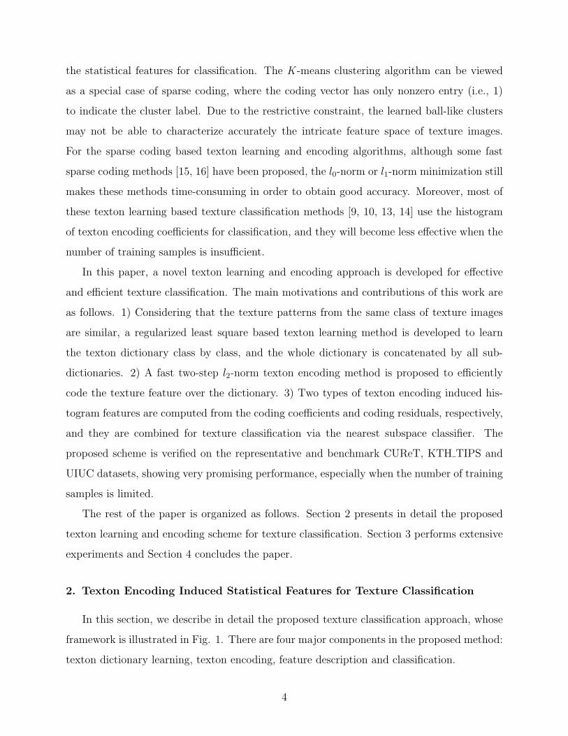
the statistical features for classification. The K -means clustering algorithm can be viewed

as a special case of sparse coding, where the coding vector has only nonzero entry (i.e., 1)

to indicate the cluster label. Due to the restrictive constraint, the learned ball-like clusters

may not be able to characterize accurately the intricate feature space of texture images.

For the sparse coding based texton learning and encoding algorithms, although some fast

sparse coding methods [15, 16] have been proposed, the l0-norm or l1-norm minimization still

makes these methods time-consuming in order to obtain good accuracy. Moreover, most of

these texton learning based texture classification methods [9, 10, 13, 14] use the histogram

of texton encoding coefficients for classification, and they will become less effective when the

number of training samples is insufficient.

In this paper, a novel texton learning and encoding approach is developed for effective

and efficient texture classification. The main motivations and contributions of this work are

as follows. 1) Considering that the texture patterns from the same class of texture images

are similar, a regularized least square based texton learning method is developed to learn

the texton dictionary class by class, and the whole dictionary is concatenated by all sub-

dictionaries. 2) A fast two-step l2-norm texton encoding method is proposed to efficiently

code the texture feature over the dictionary. 3) Two types of texton encoding induced his-

togram features are computed from the coding coefficients and coding residuals, respectively,

and they are combined for texture classification via the nearest subspace classifier. The

proposed scheme is verified on the representative and benchmark CUReT, KTH TIPS and

UIUC datasets, showing very promising performance, especially when the number of training

samples is limited.

The rest of the paper is organized as follows. Section 2 presents in detail the proposed

texton learning and encoding scheme for texture classification. Section 3 performs extensive

experiments and Section 4 concludes the paper.

2. Texton Encoding Induced Statistical Features for Texture Classification

In this section, we describe in detail the proposed texture classification approach, whose

framework is illustrated in Fig. 1. There are four major components in the proposed method:

texton dictionary learning, texton encoding, feature description and classification.

4

Training samples

Feature

extraction

Test sample

Texton

learning

Dictionary of

textons

Texton

encoding

Coefficient

histograms

Residual

histograms

Feature

extraction

Texton

encoding

Matching

Matching

Distance

fusionClassification

Texton learning

Texton encoding Feature description and classification

Coefficient

histogram

Residual

histogram

Figure 1: Framework of the proposed texton learning and encoding based texture classification method.

2.1. Texton Dictionary Learning

A dictionary of textons is to be learned from the training texture images so that they can

be used to represent the test image. Before learning the textons, the training texture images

are first converted into grey level images and normalized to have zero mean and unit standard

deviation. This process reduces the image variations caused by illumination changes. The

texture features (e.g., the MR8 feature [9], the patch feature [10] and the SIFT feature

[19]) are then extracted from the pre-processed texture images and normalized by using the

Weber’s law [9]. Suppose that at each pixel of a texture image, we extract an M -dimensional

feature vector, denoted by xi, and then for each class of texture images, we can construct

a training dataset X = [x1,x2, . . . ,xN ] ∈ RM×N , where N is the number of pixels in all

training images of this class. The dictionary of textons, denoted by D = [d1,d2, . . . ,dL] ∈

RM×L, is to be learned from the training dataset X, where dj, j = 1, 2, . . . , L, is a texton.

The dictionary D should be much more compact than X, i.e., L ≪ N , but it is expected

that all the samples in X could be well represented by the learned dictionary D.

The texture classification methods in [7, 8, 9, 10, 20, 11, 12, 13] use the K -means clustering

to learn the textons. Though the K -means clustering is easy and fast to implement, its

representation accuracy is limited because only the cluster center is used to approximate

the samples. To increase the representation accuracy, we could use the linear combination of

several textons, but not the single cluster center, to represent the sample. For example, in [14]

the sparse representation model is used to train such a dictionary by solving minD,Λ(∥X −

5

DΛ∥2F + λ∥Λ∥1), where λ is a positive constant to balance the representation error and

the sparsity of coding coefficients Λ. However, the sparse coding process is rather time

consuming. Furthermore, using sparse representation to learn the dictionary of textons often

implies that we have to use sparse representation to encode the query sample, making the

texture classification process expensive and slow.

In order to achieve high representation accuracy and efficiency simultaneously, in this

paper we propose the following texton learning model:

minD,Λ(∥X −DΛ∥2F + λ∑N

i=1∥αi∥22 + γ

∑N

i=1∥αi − µ∥22) s.t. dT

j dj = 1 (1)

where Λ = [α1,α2, . . . ,αN ] ∈ RL×N is the coding coefficient matrix of X over D and

αi, i = 1, 2, . . . , N , is the L-dimensional coding vector of xi; µ is the mean of all αi, i.e.,

µ = 1N

∑Ni=1αi; parameters λ and γ are positive scalars. In general, we require that each

texton dj is a unit vector, i.e., dTj dj = 1.

In the proposed texton learning model in Eq. (1), we use the l2-norm, instead of the

l1-norm, to characterize the coding vectors based on the following considerations. First,

since the training samples are from the same class, it is not necessary to force the encoding

coefficients to be sparse. Second, we learn a compact but not an over-complete dictionary

for each class, and l2-norm regularization is good enough to yield a stable solution to the

dictionary. Third, since we will use l2-norm regularization in the texton encoding stage

(please refer to Section 2.2), it is reasonable to also use l2-norm regularization to learn the

dictionary in the training stage. Finally, l2-norm regularization improves much the speed

in training, which is a desirable advantage. In addition, since the training samples xi from

the same class share similarities in appearance, their coding vectors should also be similar.

Therefore, in Eq. (1) we enforce their coding vectors αi to approach to their mean µ, i.e.,

minimizing∑N

i=1 ∥αi − µ∥22. This term is basically to reduce the intra-class variation for

more accurate classification.

The optimization of Eq. (1) can be easily conducted by alternatively optimizing D and

Λ. With some random initialization of D, we could first fix D and update Λ, and the

6

problem in Eq. (1) is reduced to a regularized least square problem:

αi = argminΛ(∥X −DΛ∥2F + λ∑N

i=1∥αi∥22 + γ

∑N

i=1∥αi − µ∥22)

= argminΛ(∥X −DΛ∥2F + λ∑N

i=1∥αi∥22 + γ(

∑N

i=1∥αi∥22 −N∥µ∥22)).

(2)

Let the partial derivative of Eq. (2) with respect to αi equal to 0, we have:

(DTD + λI + γI )αi −DTxi =γ

N

∑N

i=1αi. (3)

Summing up Eq. (3) from i = 1 to i = N , we have:∑N

i=1αi = (DTD + λI )−1DT

∑N

i=1xi. (4)

It is easy to derive that each coding vector αi in Λ can be analytically solved by:

αi = (DTD + λI + γI )−1(DTxi +γ

N(DTD + λI )−1DT

∑N

i=1xi). (5)

Once all the coding vectors are updated, we could fix Λ and update D. The objective

function in Eq. (1) is then reduced to minD∥X −DΛ∥2F s.t. dTj dj = 1. We update the

textons dj one by one. When updating dj, the other textons dk(k = j) are fixed. Denote by

βj the jth row of Λ. We have

dj = argmindj∥X −

∑k =j

dkβk − djβj∥2F s.t. dTj dj = 1. (6)

Let Z = X −∑

k =j dkβk, and then the above equation can be re-written as:

dj = argmindj∥Z − djβj∥2F s.t. dT

j dj = 1. (7)

By using the Lagrange multiplier, we can obtain:

dj = argmindjtr((Z − djβj)(Z − djβj)

T − γdjdTj − γ). (8)

Let the partial derivative of Eq. (8) with respect to dj equal to 0, we have:

−ZβTj + dj(βjβ

Tj − γ) = 0. (9)

It can be easily derived that the solution to Eq. (8) is

dj = ZβTj /∥ZβT

j ∥2. (10)

Once all the textons dj inD are updated, we then fixD and update the coding coefficients

Λ by using Eq. (5), and in turn fix Λ and update the dictionary D by Eq. (10). Since in

each iteration the energy function in Eq. (1) can only reduce, the alternative optimization

process will converge to a local minimum, and the desired texton dictionary D is learned.

7

2.2. Texton Encoding

By using the texton learning algorithm presented in Section 2.1, for each class k, k =

1, 2, . . . , C, we can learn a texton dictionary Dk. Then the intra-class dictionaries learned

from all the C classes can be concatenated into a dictionary Φ = [D1,D2, . . . ,DC ] to encode

the input texture feature vectors for classification. In the K -means clustering based texton

learning and encoding methods [7, 8, 9, 10, 11, 12, 13], each texture feature vector is encoded

as the label of the texton closest to it. A histogram is built by counting the frequencies of

texton labels and it is consequently used as the statistical feature to describe the texture

image.

The texton learning and encoding in the K -means clustering based methods [9, 10] is

simple but rather coarse. The proposed texton learning model in Eq. (1) can have much

higher representation accuracy than the K -means clustering method because it uses a few

textons to represent the feature vector. A corresponding texton encoding model needs to be

proposed to encode the test feature vector. Let us denote by yi the feature vector extracted

at position i of a given texture image. One may encode yi by αi = argminαi(∥yi −Φαi∥22 +

λ∥αi∥22), which is very fast to optimize because αi = P · yi and P = (ΦTΦ+ λI )−1ΦT can

be pre-calculated as a projection matrix. Different from the class-by-class dictionary learning

model in Eq. (1), where the goal is to improve the representation power ofD for a given class,

here Φ is the concatenated dictionary of all classes and our goal is to have a discriminative

encoding of yi for accurate classification. Using l2-norm to regularize αi is not effective to

achieve this goal since l2-norm tends to generate many big coefficients over different classes.

Intuitively, employing l1-norm regularization in the encoding is able to generate sparse and

more discriminative coding coefficients: αi = argminαi(∥yi−Φαi∥22+λ∥αi∥1). However, the

l1-minimization is very time consuming, particularly for the concatenated big dictionary Φ.

Though many fast l1-minimization techniques have been proposed, such as FISTA [15] and

ALM [16], it is still highly desirable if we could find an l2-minimization based texton encoding

method while preserving a certain degree of sparsity. We propose a two-step encoding scheme

to achieve this goal.

First, we project yi by using the pre-calculated projection P : αi = P · yi, and select the

p most related textons to yi from Φ by identifying the p most significant coding coefficients

8

in |αi|. Usually we set p ≤ M , where M is the dimension of the feature vector yi. Denote

by di,1,di,2, . . . ,di,p the selected p textons to yi. We can thus form a small but adaptive

sub-dictionary to yi as Φi = [di,1,di,2, . . . ,di,p].

We then encode yi over the sub-dictionary Φi by

θi = argminθi(∥yi −Φiθi∥22 + λ∥θi∥22). (11)

Clearly, this is a simple regularized least square problem as we have θi = Pi · yi and Pi =

(ΦTi Φi + λI )−1ΦT

i . Since p (p ≤ M) is generally small (please refer to Section 3.4 for more

information), the computation of θi is very fast. We can also use the conjugate gradient

method [26] to further speed up this encoding process.

The proposed two-step fast texton encoding scheme can be roughly viewed as a hybrid

l0-l2-minimization with ∥θi∥0 ≤ p. The first step selects the p textons and actually sets the

coding coefficients over the other textons as zeros. This leads to a sparse representation of

yi. The second step refines the coding coefficients over the selected p textons to make the

representation accurate.

2.3. Feature Description

By using the proposed texton encoding scheme, we could naturally define two types of

statistical histogram features to describe the texture image. The first feature descriptor

comes from the encoding coefficient θi. We normalize θi into ωi by

ωi,t = |θi,t|/∑p

q=1|θi,q|, t = 1, 2, . . . , p (12)

where ωi,t is the tth element of ωi and θi,t is the tth element of θi. Thus, for each feature

vector yi of the texture image, we have a representation vector vi, where only the entries

corresponding to the same textons as those in Φi will have non-zero values, i.e., ωi,t, while the

other entries in vi are zeros. Then we can form a histogram, denoted by hc, as one statistical

descriptor of this texture image:

hc =∑n

i=1vi (13)

where n is the number of pixels in the texture image.

9

Apart from the encoding coefficient induced histogram, we can also build another his-

togram by using the encoding residual associated with each of the selected p textons:

ei,t = ∥yi − di,tθi,t∥2, t = 1, 2, . . . , p (14)

where ei,t is the tth element of ei. Since the smaller the residual, the more important the

associated texton in representing the feature vector, we normalize ei into δi by

δi,t =1/ei,t∑pq=1 1/ei,q

, t = 1, 2, . . . , p (15)

where δi is the normalized reciprocal of encoding residual associated with Φi and δi,t is the

tth element of δi. With δi we can readily re-construct the encoding residual vector of yi over

Φ, denoted by si. That is, in si the entries corresponding to the same textons as those in Φi

will have the same values as in δi, and the remaining entries in si are zeros. Finally, for each

feature vector yi of the texture image, we have an encoding residual induced vector si, and

then we can form a histogram, denoted by hr, as another statistical descriptor of the texture

image:

hr =∑n

i=1si. (16)

Histograms hc and hr are two statistical descriptors induced by the encoding coefficients

and encoding residuals, respectively. Fig. 2 shows two texture images of different classes and

their histograms hc and hr. We can see that the histogram features of different classes are

very different. Meanwhile, the two types of histograms of the same texture image, hc and hr,

also have enough difference, implying that they have complementary information for texture

classification.

2.4. Classification

Suppose there are C classes of textures in the dataset, and there are l training samples per

class. Denote by Hc = [hc,1,hc,2, . . . ,hc,l] and Hr = [hr,1,hr,2, . . . ,hr,l] the sets of encoding

coefficient histograms and encoding residual histograms for one class, respectively. For a test

texture image y, we first build its two histogram descriptors, denoted by hyc and hy

r , and

then we use the nearest subspace classifier (NSC) to classify y. We project hyc and hy

r into

the subspaces spanned by Hc and Hr, respectively, as follows:

ρc = (HTc Hc)

−1HTc h

yc ;ρr = (HT

r Hr)−1HT

r hyr (17)

10

0 500 1000 1500 2000 25000

10

20

30

40

50

60

70

80

90

0 500 1000 1500 2000 25000

10

20

30

40

50

60

70

0 500 1000 1500 2000 25000

50

100

150

200

250

300

350

0 500 1000 1500 2000 25000

50

100

150

200

250

Figure 2: Two texture images (the left column) and their histogram features hc and hr (the right two

columns).

The projection residuals can be computed as:

errc = ∥hyc −Hcρc∥2; errr = ∥hy

r −Hrρr∥2. (18)

Using Eqs. (17) and (18), for each of the C classes, we can calculate the residuals, and

then form two vectors errc and errr which contain the projection residuals from all classes.

By NSC, with either errc or errr, we can classify y by either identity(y) = argminkerrc(k)

or identity(y) = argminkerrr(k), k = 1, 2, . . . , C. To exploit the discriminative information

from both coding coefficients and coding residuals, we fuse errc and errr for classification.

Here we adopt the simple weighted average method for fusion:

errf = w · errc + (1− w) · errr, 0 ≤ w ≤ 1 (19)

where w is the weight and it can be trained from the training dataset with the ”leave-one-out”

strategy. Then the classification can be done via

identity(y) = argminkerrf (k), k = 1, 2, . . . , C. (20)

3. Experimental Evaluation

3.1. Texture Datasets

To demonstrate the effectiveness of our proposed texture classification method, three

representative and benchmark texture datasets are used in our experiments: CUReT [17],

11

KTH TIPS [18] and UIUC [11]. In accordance with other studies which use the CUReT

dataset for classification, we use the same subset of CUReT provided by Varma and Zisserman

[9], which contains 61 classes and 92 images per class. There are a few factors that make the

CUReT dataset challenging. It has both large inter-class similarity and intra-class variation.

The images were captured under unknown viewpoint and illumination. Fig. 3 shows some

sample images from two different classes in the CUReT dataset. One can see that their

appearances are very similar.

Figure 3: Each row shows three sample images of one texture class in the CUReT dataset.

A drawback of the CUReT dataset is its lack of large scale variations. Hence, the

KTH TIPS dataset was established to supplement CUReT additional sample images with

scale variations. The KTH TIPS dataset contains 10 classes of materials which are presented

in the CUReT dataset. Each class was imaged at 9 different distances while at each distance

the images were captured under 3 different directional illuminations and 3 different view-

points. As a result, 81 texture images are provided for each class. In our experiment, we

treat it as a stand-alone dataset, following the setting in [12]. Fig. 4 shows some texture

images of two different classes in the KTH TIPS dataset.

The UIUC dataset contains 25 classes, each having 40 images. A major property of the

UIUC dataset is that there are some significant scale and viewpoint changes as well as some

non-rigid deformations in its images. Although the UIUC dataset has less severe lighting

variations than the CUReT dataset, in terms of intra-class variations of appearance, it is the

most challenging one among the commonly used datasets for texture classification. Fig. 5

12

shows some texture images in the UIUC dataset.

Figure 4: Each row shows three sample images of one texture class in the KTH TIPS dataset, which has

large scale variations.

Figure 5: Each row shows three sample images of one texture class in the UIUC dataset, which has large

viewpoint changes and non-rigid deformations.

3.2. Parameter Selection and Implementation Details

The evaluation methodology on the three datasets is as follows: l images are randomly

chosen per class for training and the remaining images are used for testing. On CUReT, 6,

12, 23 and 46 images per class are randomly chosen to form the training set; on KTH TIPS,

5, 10, 20, 30 and 40 images per class are randomly chosen to form the training set; on UIUC,

5, 10, 15 and 20 training images are randomly chosen per class to form the training set. For

each setting, the experiments were run 100 times and the average classification accuracy is

13

reported. In texton dictionary learning of our model, parameters λ and γ in Eq. (1) are

set to 2 × 10−4. In texton encoding with the learned dictionary, parameter λ is also set to

2× 10−4. These parameters are fixed on all the three texture datasets.

On the CUReT and KTH TIPS datasets, we employed the MR8 feature [9] to represent

the texture image for texton learning and encoding. For each class, L = 40 textons are

learned. The MR8 feature vector is 8-dimensional, i.e., M = 8, and thus in the two-step fast

texton encoding process we choose p = 7 textons to form the sub-dictionary for encoding.

Since the texture images in the UIUC dataset are with large scale and viewpoint vari-

ations, using the MR8 feature alone cannot achieve good classification performance. Many

existing texture classification methods [11, 12, 13, 21] employ multiple types of features on

the UIUC texture dataset. For example, in [11], the SPIN and RIFT descriptors are combined

to learn the dictionary for classification, while in [12] the SPIN, RIFT and SIFT descriptors

are combined to learn the dictionary. In [13] and [21], the combination of sorted random

projection features and the combination of three kinds of multi-fractal spectrums are used

to classify the UIUC dataset, respectively. Here we employ the MR8 feature [9] and the

SIFT feature [19] to represent the texture images in the UIUC dataset to address their large

scale and viewpoint variations. For each class, 100 MR8 textons and 100 SIFT textons per

class are learned, respectively. Their histogram features are combined to classify the texture

images. For the MR8 feature, p = 7 is set in texton encoding. For the 128-dimensional SIFT

feature, we set p = 100.

For the projection residual fusion in NSC based classification, the weight w is determined

by applying the leave-one-out method on the training set. When 6, 12, 23 and 46 training

samples per class are used in the experiments on the CUReT dataset, the values of w are 0.5,

0.65, 0.4 and 0.5, respectively. On the KTH TIPS dataset, when 5, 10, 20, 30 and 40 training

samples per class are used, the weights are 0.65, 0.95, 0.65, 0.75 and 0.65, respectively. On

the UIUC dataset, when 5, 10, 15 and 20 randomly chosen training samples are used, the

weights are 0.6, 0.75, 0.75 and 0.55, respectively.

3.3. Experimental Results

Evaluation of the proposed method : We denote by TEISF c, TEISF r and TEISF f the

proposed texton encoding induced statistical feature (TEISF) based methods with only the

14

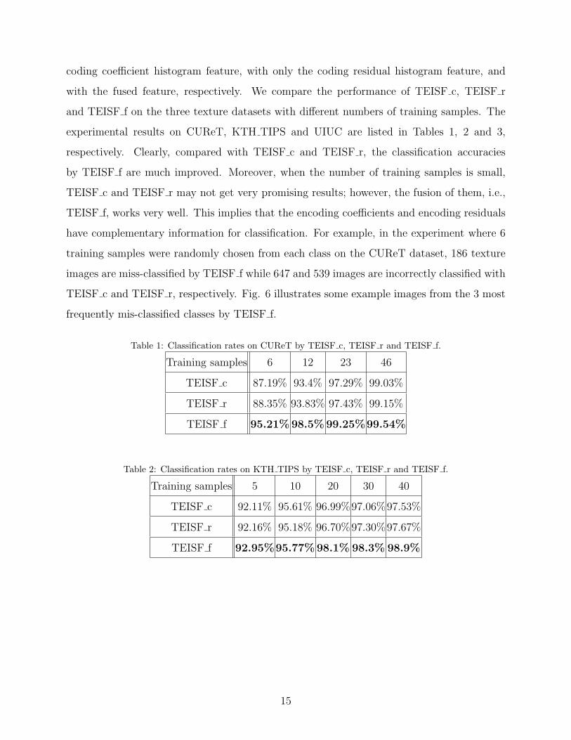
coding coefficient histogram feature, with only the coding residual histogram feature, and

with the fused feature, respectively. We compare the performance of TEISF c, TEISF r

and TEISF f on the three texture datasets with different numbers of training samples. The

experimental results on CUReT, KTH TIPS and UIUC are listed in Tables 1, 2 and 3,

respectively. Clearly, compared with TEISF c and TEISF r, the classification accuracies

by TEISF f are much improved. Moreover, when the number of training samples is small,

TEISF c and TEISF r may not get very promising results; however, the fusion of them, i.e.,

TEISF f, works very well. This implies that the encoding coefficients and encoding residuals

have complementary information for classification. For example, in the experiment where 6

training samples were randomly chosen from each class on the CUReT dataset, 186 texture

images are miss-classified by TEISF f while 647 and 539 images are incorrectly classified with

TEISF c and TEISF r, respectively. Fig. 6 illustrates some example images from the 3 most

frequently mis-classified classes by TEISF f.

Table 1: Classification rates on CUReT by TEISF c, TEISF r and TEISF f.

Training samples 6 12 23 46

TEISF c 87.19% 93.4% 97.29% 99.03%

TEISF r 88.35% 93.83% 97.43% 99.15%

TEISF f 95.21%98.5%99.25%99.54%

Table 2: Classification rates on KTH TIPS by TEISF c, TEISF r and TEISF f.

Training samples 5 10 20 30 40

TEISF c 92.11% 95.61% 96.99%97.06%97.53%

TEISF r 92.16% 95.18% 96.70%97.30%97.67%

TEISF f 92.95%95.77%98.1% 98.3% 98.9%

15

Table 3: Classification rates on UIUC by TEISF c, TEISF r and TEISF f.

Training samples 5 10 15 20

TEISF c 91.05% 95.30% 97.38% 98.18%

TEISF r 93.29% 95.82% 97.65% 98.22%

TEISF f 94.37%98.38%99.35%99.54%

Figure 6: Example images misclassified by the TEISF f method in the CUReT dataset. The left 3 columns

show some test texture images while the right 3 columns show images from the class that these test images

are misclassified to. Specifically, “Styrofoam”(top), “Aquarium stones”(middle) and “Moss”(bottom) are

misclassified to “Cork”, “Aluminum foil” and “Soleirolia plant”, respectively. From these example images

one can see that the misclassified test images are often perceptually similar to the template images.

Comparison evaluation: We compare our methods with representative and recently de-

veloped texture classification methods [1, 3, 35, 36, 5, 6, 9, 10, 20, 18, 11, 12, 13]. Since

many competing methods do not have publically released source codes available, we cropped

the results from their original papers, or we asked the authors to provide the results. If the

classification accuracies of some competing methods are not available, we use symbol ’–’ to

represent the missing results. Different competing methods may use different classifiers, e.g.,

the nearest neighbor classifier with the χ2-distance in [1, 3, 9, 10, 20, 21, 5], SVM classifier

in [18, 12, 13], etc. For LBP [1], CLBP [3], and VZ MR8 [9], we coupled them with the NSC

classifier, which gives better classification rates than the nearest neighbor classifier with the

16

χ2-distance as in the original papers.

Table 4 compares the competing texture classification methods on the three texture

datasets when enough training samples are available (46 for CUReT, 40 for KTH TIPS and

20 for UIUC). One can see that when there are enough training samples, most of the methods

can achieve good classification accuracy. The proposed TEISF f method works the best on

the CUReT and UIUC datasets, and it is only slightly worse than Liu et al.’s method [13] by

a gap of 0.39 pp (percentage point) on the KTH TIPS dataset. In this experiment, the gain

of TEISF f over TEISF c and TEISF r is not significant because TEISF c and TEISF r can

also achieve good results when enough training samples are available.

By decreasing the number of training samples per class, in Tables 5, 6 and 7 we present the

classification accuracies on the three datasets, respectively. (Note that not all the competing

methods employed in Table 4 are reported in Tables 5, 6 and 7 since some results are not

available.) From these tables, we can readily make the following findings. 1) The proposed

TEISF f achieves the best classification accuracy in almost every case. 2) With the decrease

of the number of training samples, the advantage of TEISF f over other methods is getting

more and more obvious. 3) TEISF f is much more robust to the number of training samples

than other competing methods. For example, on the CUReT dataset, TEISF f’s classification

accuracies are 95.21%, 98.5%, 99.25% and 99.54% with 6, 12, 23 and 46 training samples

per class, respectively. From 46 training samples per class to 6 training samples per class,

the drop in classification rate is only 4.3 pp. However, for other methods, the drop is often

more than 10 pp. 4) Some methods may work well on one dataset but not so well on other

datasets. For example, Xu et al.’s method [5, 21] has good accuracy on the UIUC dataset,

whereas its accuracy on the CUReT dataset is not so good. In comparison, the proposed

TEISF f can obtain good results across all datasets. In addition, in Fig. 7 we plot the curves

of classification rate vs. number of training samples on the three datasets by TEISF f. The

curves by VZ MR8 [9]+ NSC, CLBP [3]+NSC and the method in [13] are also plotted for

comparison. Clearly, the proposed method is much more robust than other methods to the

number of training samples.

The speed of one algorithm in processing one query sample is very important for its

practical usage. In the texton encoding stage of our TEISF f algorithm, the time complexity

17

of selecting the p most related textons is O((CL)2), and the complexity of solving the least

square problem in Eq. (11) isO(p2M), where CL is the number of textons in the concatenated

dictionary Φ, p is the number of the selected textons in the texton encoding stage and M is

the dimension of the texture feature vector. Hence, the time complexity of texton encoding in

the proposed TEISF f method is O(n(CL)2+np2M), where n is the number of input feature

vectors of a test image. In the feature description stage, since at each pixel in the image there

are CL operations and 4Mp+ CL operations to form the coefficient histogram and residual

histogram, respectively, the time complexity of feature description is O(nMp + nCL). In

the classification stage, the time complexity of computing the projection residuals and fusing

them is O(l2CL), where l is the number of training images per class.

Let us then compare the average running time of the proposed TEISF f method with

the K -means clustering based VZ MR8 method [9] and the l1-sparsity based texton learning

method [14], where a texton encoding procedure is employed to classify the query sample. On

the CUReT and KTH TIPS datasets, 40 textons per class are used in the texton encoding of

the proposed method, and on the UIUC dataset, 100 MR8 textons and 100 SIFT textons per

class are employed, respectively. All experiments were performed in the Matlab programming

environment on a laptop with a 2.30 GHz quad-core Intel processor and 8 GB memory. The

average running time is listed in Table 8. One can see that TEISF f is much faster than the

l1-sparsity based method [14]. Compared with the K -means clustering based method in [9],

although the proposed method is slower, it can obtain much higher classification rate (please

refer to Tables 5, 6 and 7). It should be noted that on the CUReT and KTH TIPS datasets,

we employed only the MR8 features to learn the dictionary and encode the coefficient, while

on the UIUC dataset we employed both the MR8 and SIFT features for dictionary learning

and coefficient encoding. Therefore, the difference of running time between VZ MR8 [9] and

TEISF f on the UIUC dataset is larger than that on the CUReT and KTH TIPS datasets.

Overall, the proposed method can achieve a good trade-off between the classification rate

and the computational complexity.

3.4. Effects of Parameters L and p

In this subsection, we study the effects of parameters L and p on the final classification

accuracy. Parameter L is the number of textons per class in the dictionary, which controls

18

Table 4: Texture classification rates by different methods when the number of training samples is relatively

large.

CUReT(46)KTH TIPS(40)UIUC(20)

LBP [1]+NSC 99.11% 97.19% 80.3%

CLBP [3]+NSC 96.19% 96.74% 95.18%

NRLBP [35]+NSC 95.84% 97.57% 81.48%

DRLBP [36]+NSC 92.10% 83.04% 68.88%

VZ MR8 [9]+NSC 98.17% 97.06% 96.74%

VZ Patch [10] 98.03% 92.40% 97.83%

Hayman et al. [18] 98.46% 94.80% 92.00%

Lazebnik et al. [11] 72.50% 91.13% 93.62%

Zhang et al. [12] 95.30% 96.10% 98.70%

Varma and Garg [20] 97.50% 95.40%

Crosier and Griffin [6] 98.60% 98.50% 98.80%

Xu et al. [5] 98.60%

Liu et al. [13] 99.37% 99.29% 98.56%

TEISF c 99.03% 97.53% 98.18%

TEISF r 99.05% 97.67% 98.22%

TEISF f 99.54% 98.9% 99.54%

2 4 6 8 10 120.5

0.55

0.6

0.65

0.7

0.75

0.8

0.85

0.9

0.95

1

Number of training samples

Cla

ssific

atio

n a

ccu

racy

TEISF−fVZ−MR8+NSCCLBP+NSCLiu et al.

3 5 7 9 11 130.65

0.7

0.75

0.8

0.85

0.9

0.95

1

Number of training samples

Cla

ssific

atio

n a

ccu

racy

TEISF−fVZ−MR8+NSCCLBP+NSCLiu et al.

3 5 7 9 11 13

0.65

0.7

0.75

0.8

0.85

0.9

0.95

1

Number of training samples

Cla

ssific

atio

n a

ccu

racy

TEISF−fVZ−MR8+NSCCLBP+NSCLiu et al.

Figure 7: The curves of classification rate vs. number of training samples by TEISF f, VZ MR8 [9]+NSC,

CLBP [3]+NSC and Liu et al.’s method [13] on CUReT (left), KTH TIPS (middle) and UIUC (right).

19

Table 5: Classification rates on the CUReT dataset with different numbers of training samples.

Training samples 6 12 23 46

LBP [1]+NSC 82.25% 91.71% 96.24% 99.11%

CLBP [3]+NSC 79.75% 90.51% 94.47% 96.19%

NRLBP [35]+NSC 79.93% 90.46% 94.05% 95.84%

DRLBP [36]+NSC 62.86% 76.08% 84.50% 92.10%

VZ MR8 [9]+NSC 86.33% 92.79% 96.45% 98.17%

Varma and Garg [20] 81.67% 89.74% 94.69% 97.5%

Liu et al. [13] 86.48% 96.43% 97.71% 99.37%

TEISF c 87.19% 93.4% 97.29% 99.03%

TEISF r 88.35% 93.83% 97.43% 99.15%

TEISF f 95.21%98.5%99.25%99.54%

Table 6: Classification rates on the KTH TIPS dataset with different numbers of training samples.

Training samples 5 10 20 30 40

LBP [1]+NSC 72.50% 85.41% 94.12%95.73% 97.19%

CLBP [3]+NSC 78.51% 87.69% 94.78%96.05% 96.74%

NRLBP [35]+NSC 73.43% 88.92% 94.62%95.71% 97.57%

DRLBP [36]+NSC 59.80% 68.94% 75.80%80.49% 83.04%

VZ MR8 [9]+NSC 90.46% 93.45% 95.32%95.70% 97.06%

Liu et al. [13] 80.90% 89.49% 96.40% 98.4%99.29%

TEISF c 92.11% 95.61% 96.99%97.06% 97.53%

TEISF r 92.16% 95.18% 96.70%97.30% 97.67%

TEISF f 92.95%95.77%98.1% 98.3% 98.9%

the capacity of the dictionary to represent the texture appearance. We conduct a series of

experiments with different numbers of textons on the three texture datasets. Fig. 8 plots

the curves of classification rate v.s. number of leaned textons from each class. One can see

that in the proposed TEISF f method the number of learned textons, which ranges from 20

20

Table 7: Classification rates on the UIUC dataset with different numbers of training samples.

Training samples 5 10 15 20

LBP [1]+NSC 43.34% 63.15% 74.15% 80.3%

CLBP [3]+NSC 76.73% 89.5% 94% 95.18%

NRLBP [35]+NSC 44.99% 66.74% 76.12% 81.48%

DRLBP [36]+NSC 36.68% 54.97% 62.85% 68.88%

VZ MR8 [9]+NSC 86.54% 93.56% 95.71% 96.74%

VZ Patch [10] 90.17% 95.18% 96.94% 97.83%

Lazebnik et al. [11] 84.77% 90.17% 92.42% 93.62%

Varma and Garg [20] 85.35% 91.64% 94.09% 95.4%

Xu et al. [5] 93.42% 96.95% 98.01% 98.60%

Liu et al. [13] 90.96% 96.00% 97.59% 98.56%

TEISF c 91.05% 95.30% 97.38% 98.18%

TEISF r 93.29% 95.82% 97.65% 98.22%

TEISF f 94.37%98.38%99.35%99.54%

Table 8: Average running time of the three texton encoding based methods on the CUReT, KTH TIPS and

UIUC texture datasets.

CUReTKTH TIPS UIUC

VZ MR8 [9] 7.3s 4.2s 80.9s

l1-sparsity [14] 133.2s 53.3s 1254.5s

TEISF f 13.6s 8.0s 217.6s

to 100, has little effect on the final classification accuracy.

The parameter p controls the number of selected textons in the texton encoding stage.

In some sense it controls the sparsity of coding coefficients in the texton encoding. Fig. 9

shows the classification rates under different numbers of selected textons on the CUReT,

KTH TIPS and UIUC datasets, respectively. Note that two dictionaries (for MR8 and SIFT

features) are used on the UIUC dataset. Thus in the right sub-figure of Fig. 9, the x-axis

labels a pair of numbers of the selected MR8 and SIFT textons. From these figures, we can

21

observe that when p is large (e.g., p > 15 for the MR8 feature on the CUReT dataset), the

sparsity of coding coefficients is reduced and the classification rate also decreases. When p

is very small (e.g., p < 5 for the MR8 feature on the CUReT dataset), the representation is

not accurate so that the classification rate is not very good, either. Empirically, when p is

slightly less than the feature dimensionality (e.g., p = 7 for the 8-dimensional MR8 feature),

a good balance of representation accuracy and sparsity is reached so that good classification

rate can be obtained. For example, on the CUReT dataset, with 46 training samples per

class, when 7 textons are chosen, a classification rate of 99.54% can be obtained.

20 40 60 80 1000.95

0.955

0.96

0.965

0.97

0.975

0.98

0.985

0.99

0.995

1

Number of learned textons

Cla

ss

ific

ati

on

ac

cu

rac

y

6 training samples12 training samples23 training samples46 training samples

20 40 60 80 1000.91

0.92

0.93

0.94

0.95

0.96

0.97

0.98

0.99

Number of learned textons

Cla

ss

ific

ati

on

ac

cu

rac

y

5 training samples10 training samples20 training samples30 training samples40 training samples

20 40 60 80 1000.94

0.95

0.96

0.97

0.98

0.99

1

Number of learned textons

Cla

ss

ific

ati

on

ac

cu

rac

y

5 training samples10 training samples15 training samples20 training samples

Figure 8: The curves of classification rate vs. number of learned textons from each class of training samples

by TEISF f on CUReT (left), KTH TIPS (middle) and UIUC (right).

3 5 7 10 15 20 25 35 50 70 1000.94

0.95

0.96

0.97

0.98

0.99

1

Number of selected textons

Cla

ssif

icati

on

accu

racy

6 training samples12 training samples23 training samples46 training samples

3 5 7 10 15 20 25 35 50 70 1000.91

0.92

0.93

0.94

0.95

0.96

0.97

0.98

0.99

Number of selected textons

Cla

ssif

icati

on

accu

racy

5 training samples10 training samples20 training samples30 training samples40 training samples

(3,60) (5,80) (7,100) (10,120) (15,140) (20,160) (25,180) (35,200) (50,220) (70,240)(100,260)0.93

0.94

0.95

0.96

0.97

0.98

0.99

1

Number of selected textons

Cla

ssif

icati

on

accu

racy

5 training samples10 training samples15 training samples20 training samples

Figure 9: The curves of classification rate vs. number of selected textons in the texton encoding stage by

TEISF f on CUReT (left), KTH TIPS (middle) and UIUC (right).

4. Conclusions

We proposed a texton encoding based texture classification method, which is simple to

implement and shows very promising performance. The textons were learned to ensure the

22

representation accuracy while reducing the within-class variance. A two-step texton encoding

scheme was then proposed to encode efficiently the texture feature over the learned dictionary

while preserving certain sparsity. Two types of statistical features, namely, coding coefficient

induced histogram and coding residual induced histogram, were then defined, with which

the nearest subspace classifier was applied for texture classification. The proposed texton

encoding induced statistical feature (TEISF) method was validated on three representative

and benchmark texture datasets: CUReT, KTH TIPS and UIUC. The experimental results

demonstrated that TEISF achieves very good texture classification performance, especially

when the number of training samples is small.

References

[1] T. Ojala, M. Pietikainen, T. Maenpaa, Multi-resolution gray-scale and rotation invariant

texture classification with local binary patterns, IEEE Trans. on Pattern Analysis and

Machine Intelligence. 7(24)(2002)971-987.

[2] S. Liao, W. K. Law, C. S. Chung, Dominant local binary pattern for texture classifica-

tion, IEEE Trans. on Image Processing. 18(5)(2009)1107-1118.

[3] Z. H. Guo, L. Zhang, D. Zhang, A completed modeling of local binary pattern operator

for texture classification, IEEE Trans. on Image Processing. 19(6)(2010) 1657-1663.

[4] Z. H. Guo, L. Zhang, D. Zhang, Rotation invariant texture classification using LBP

variance (LBPV) with global matching, Pattern Recognition. 43(3)(2010) 706-719.

[5] Y. Xu, X. Yang, H. Ling, H. Ji, A new texture descriptor using multifractal analysis in

multi-orientation wavelet pyramid, in Proc. Computer Vision and Pattern Recognition,

2010, pp. 161-168.

[6] M. Crosier, L. Griffin, Using basic image features for texture classification, International

Journal of Computer Vision. 88(3)(2010)447-460.

[7] T. Leung, J. Malik, Representing and recognizing the visual appearance of ma-

terials using three-dimensional textons, International Journal of Computer Vision.

43(1)(2001)29-44.

23

[8] O. G. Cula, K. J. Dana, 3D texture recognition using bidirectional feature histograms,

International Journal of Computer Vision. 59(1)(2004)33-60.

[9] M. Varma, A. Zisserman, A statistical approach to material classification from single

images, International Journal of Computer Vision. 62(2)(2005)61-81.

[10] M. Varma, A. Zisserman, A statistical approach to material classification using im-

age patch examplars, IEEE Trans. on Pattern Analysis and Machine Intelligence.

31(11)(2009)2032-2047.

[11] S. Lazebnik, C. Schmid, J. Ponce, A sparse texture representation using local affine

regions, IEEE Trans. on Pattern Analysis and Machine Intelligence. 27(8)(2005)1265-

1278.

[12] J. Zhang, M. Marszalek, S. Lazebnik, C. Schmid, Local features and kernels for classi-

fication of texture and object categories: a comprehensive study. International Journal

of Computer Vision. 73(2)(2007)213-238.

[13] L. Liu, P. Fieguth, G. Y. Kuang, H. B. Zha, Sorted random projections for robust

texture classification, in Proc. International Conference on Computer Vision, 2011, pp.

391-398.

[14] J. Xie, L. Zhang, J. You, D. Zhang, Texture classification via patch-based sparse texton

learning, in Proc. International Conference Image Processing, 2010, pp. 2737-2740.

[15] A. Beck, M. Teboulle, A fast iterative shrinkage-thresholding algorithm for linear inverse

problems, SIAM Journal on Imaging Sciences. 2(1)(2009)183-202.

[16] J. Yang, Y. Zhang, Alternating direction algorithms for l1-problems in compressive sens-

ing, SIAM Journal on Scientific Computing. 33(1)(2011)250-278.

[17] K. Dana, B. van Ginneken, S. K. Nayar, J. J. Koenderink, Reflectance and texture of

real world surfaces, ACM Trans. on Graphics. 18(1)(1999)1-34.

[18] E. Hayman, B. Caputo, M. Fritz, J. O. Eklundh, On the significance of real-world

conditions for material classification, in Proc. European Conference Computer Vision,

2004, pp. 253-266.

24

[19] D. Lowe, Distinctive image features from scale-invariant features, International Journal

of Computer Vision. 60(2)(2004)91-110.

[20] M. Varma, R. Garg, Locally invariant fractal features for statistical texture classification,

in Proc. International Conference Computer Vision, 2007, pp.1-8.

[21] Y. Xu, H. Ji, C. Fermuller, Viewpoint invariant texture description using fractal analysis,

International Journal of Computer Vision. 83(1)(2009)85-100.

[22] M. Varma, A. Zisserman, Classifying images of materials: achieving viewpoint and

illumination independence, in Proc. European Conference Computer Vision, 2002, pp.

255-271.

[23] M. Varma, A. Zisserman, Texture classification: are filter banks necessary? in Proc.

Computer Vision and Pattern Recognition, 2003, pp. 691-698.

[24] K. Skretting, J. H. Husøy, Texture classification using sparse frame based representa-

tions, EURASIP Journal. on Applied Signal Processing. (2006).

[25] J. Mairal, F. Bach, J. Ponce, G. Sapiro, A. Zisserman, Discriminative learned dictionaries

for local image analysis, in Proc. Computer Vision and Pattern Recognition, 2008, pp.

1-8.

[26] K. Tanabe, Conjugate-gradient method for computing the Moore-Penrose inverse and

rank of a matrix, Journal of Optimization Theory and Applications. 22(1)(1977) 1-23.

[27] W. Johnson, J. Lindenstrauss, Extensions of Lipschitz mappings into a Hilbert space,

in Proc. Conference in Modern Analysis and Probability, 1984, pp. 189-206.

[28] F. Bianconi, A. Fernandez, A unifying framework for LBP and related methods, in Local

Binary Patterns: New Variants and Applications, Springer, 2014, pp. 17-46

[29] N. P. Doshi, G. Schaefer, Dominant multi-dimensional local binary patterns, in Proc.

Conference on Signal Processing, Communications and Computing, 2013, pp. 1-6.

[30] M. J. Gangeh, A. Ghodsi, M. S. Kamel, Dictionary learning in texture classification, in

Proc. Conference on Image Analysis and Recognition, 2011, pp. 335-343.

25

[31] J. van Gemert, C. J. Veenman, A. W.M. Smeulders, J. M. Geusebroek, Visual word am-

biguity, in IEEE Trans. on Pattern Analysis and Machine Intelligence. 32(7)(2010)1271-

1283.

[32] Y. Guo, G. Zhao, M. Pietikainen, Discriminant features for texture description, in Pat-

tern Recognition, 45(10)(2012):3825-3843.

[33] L. Liu, L. Wang, X. Liu, In defense of soft-assignment coding, in Proc. International

Conference on Computer Vision, 2011, pp. 2486-2493.

[34] L. Nanni, A. Lumini, S. Brahnam, Local binary patterns variants as texture descriptors

for medical image analysis, in Artificial Intelligence in Medicine, 49(2)(2010)117-125.

[35] J. F. Ren, X. D. Jiang, J. S. Yuan, Noise-resistant local binary pattern with an embedded

error-correction mechanism, in IEEE Trans. on Image Processing. 22(10)(2013)4049-

4060.

[36] A. Satpathy, X. D. Jiang, H. L. Eng, LBP based edge-texture features for object recog-

nition, in IEEE Trans. on Image Processing. 23(5)(2014)1953-1964.

26