○E

Imaging the Plate Interface in the CascadiaSeismogenic Zone: New Constraints fromOffshore Receiver Functionsby Helen A. Janiszewski and Geoffrey A. Abers

Online Material: Table of station parameters.

INTRODUCTION

The Cascadia subduction zone, where the Juan de Fuca (JdF)plate subducts beneath North America, has paleoseismic evi-dence ofMw ∼9:0 megathrust earthquakes (Nelson et al., 1995;Goldfinger et al., 2003). However, there are virtually no instru-mentally recorded thrust-zone earthquakes, hence the locationand behavior of the seismogenic zone is known only indirectly.Temperature has been proposed to control seismogenesis withdepth, assuming that the locked zone extends from the trench orthe 150°C isotherm down-dip to the 350°C isotherm, with atransition zone extending to 450°C (Hyndman andWang, 1993;Oleskevich et al., 1999; Cozzens and Spinelli, 2012). These mod-els generally place the down-dip edge of the locked zone near thecoastline. Inversions of onshore Global Positioning System dataalso can be used to determine the locking behavior and place thelocked zone offshore (e.g., McCaffrey et al., 2013).

Onshore receiver function (RF) studies have imaged an east-ward-dipping low-velocity zone (LVZ) with high VP=V S betweenthe coastline and depths of 45 km (Rondenay et al., 2001; Nich-olson et al., 2005; Abers et al., 2009; Audet et al., 2009). Thisstructure has been interpreted as overpressured pore fluids, meta-morphosed sediments, or a combination thereof at or just abovethe top of the subducting oceanic crust (Abers et al., 2009; Hansenet al., 2012). Because of this uncertainty, it is unclear if an LVZshould continue up-dip through the locked zone, since fluid pres-sure and metamorphism should vary differently with depth (e.g.,Hacker et al., 2003; Liu and Rice, 2007; Saffer and Tobin, 2011).However, existing RF images only sample the plate boundarydeeper than the locked zone because past broadband arrays are onland. Brillon et al. (2013) analyze RFs from two ocean-bottomseismometers (OBSs) offshore of Vancouver Island, but poor dataquality at these stations contributes to large uncertainties.

Receiver funtions are difficult to calculate from OBS in-struments, because water column multiples interfere with otherarrivals and noise is high particularly on horizontal components(Leahy et al., 2010; Bostock and Trehu, 2012; Ball et al., 2014).The Cascadia Initiative (CI) is a prime opportunity to revisit this

challenge (Toomey et al., 2014). In particular, the new trawl-resistant-mount (TRM) OBS design not only allows the instru-ments to be deployed in shallow water, but also greatly reduceshorizontal-component noise (Webb et al., 2013). In this article,we evaluate the ability of all sites of the CI array to calculate RFs,and we focus on results from the 19 OBSs deployed off thecoast of Grays Harbor,Washington. These extend the onshoreCascadia Arrays for Earthscope (CAFE) broadband array(Abers et al., 2009) offshore, allowing direct comparisons.

DATA PROCESSING

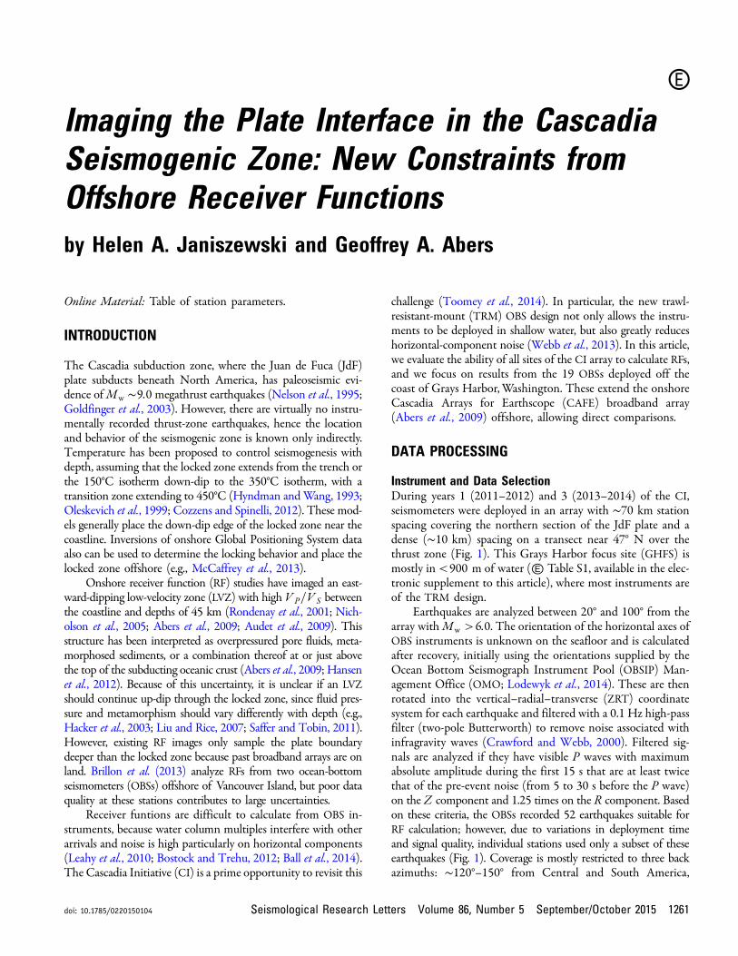
Instrument and Data SelectionDuring years 1 (2011–2012) and 3 (2013–2014) of the CI,seismometers were deployed in an array with ∼70 km stationspacing covering the northern section of the JdF plate and adense (∼10 km) spacing on a transect near 47° N over thethrust zone (Fig. 1). This Grays Harbor focus site (GHFS) ismostly in <900 m of water (Ⓔ Table S1, available in the elec-tronic supplement to this article), where most instruments areof the TRM design.

Earthquakes are analyzed between 20° and 100° from thearray withMw >6:0. The orientation of the horizontal axes ofOBS instruments is unknown on the seafloor and is calculatedafter recovery, initially using the orientations supplied by theOcean Bottom Seismograph Instrument Pool (OBSIP) Man-agement Office (OMO; Lodewyk et al., 2014). These are thenrotated into the vertical–radial–transverse (ZRT) coordinatesystem for each earthquake and filtered with a 0.1 Hz high-passfilter (two-pole Butterworth) to remove noise associated withinfragravity waves (Crawford and Webb, 2000). Filtered sig-nals are analyzed if they have visible P waves with maximumabsolute amplitude during the first 15 s that are at least twicethat of the pre-event noise (from 5 to 30 s before the P wave)on the Z component and 1.25 times on the R component. Basedon these criteria, the OBSs recorded 52 earthquakes suitable forRF calculation; however, due to variations in deployment timeand signal quality, individual stations used only a subset of theseearthquakes (Fig. 1). Coverage is mostly restricted to three backazimuths: ∼120°–150° from Central and South America,

doi: 10.1785/0220150104 Seismological Research Letters Volume 86, Number 5 September/October 2015 1261

∼220°–240° from the southwestern Pacific, and ∼270°–300°from Japan and the Aleutians (Fig. 1, inset). We also calculateRFs during the same time period at three nearby onshore sta-tions for data quality comparison (e.g., hexagons in Fig. 1).

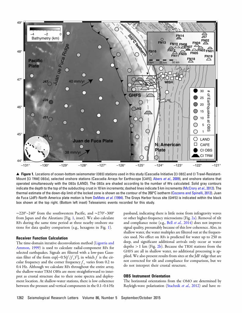
Receiver Function CalculationThe time-domain iterative deconvolution method (Ligorria andAmmon, 1999) is used to calculate radial-component RFs forselected earthquakes. Signals are filtered with a low-pass Gaus-sian filter of the form exp�−0:5�f =f c�2�, in which f is the cir-cular frequency and the corner frequency f c varies from 0.2 to0.4 Hz. Although we calculate RFs throughout the entire array,the shallow-water TRM OBSs are more straightforward to inter-pret as crustal structure due to their noise spectra and deploy-ment location. At shallow-water stations, there is low coherencebetween the pressure and vertical components in the 0.1–0.4 Hz

passband, indicating there is little noise from infragravity wavesor other higher-frequency microseisms (Fig. 2a). Removal of tiltand compliance noise (e.g., Bell et al., 2014) does not improvesignal quality, presumably because of this low coherence. Also, inshallow water, the water multiples are filtered out at the frequen-cies used. No effect on RFs is predicted for water up to 250 mdeep, and significant additional arrivals only occur at waterdepths >1 km (Fig. 2b). Because the TRM stations from theGHFS are all in shallow water, no additional processing is ap-plied. We also present results from sites at the JdF ridge that arenot corrected for tilt and compliance for comparison, but wedo not interpret their crustal structure.

OBS Instrument OrientationThe horizontal orientations from the OMO are determined byRayleigh-wave polarization (Stachnik et al., 2012) and have re-

# of Earthquakes at O

BS

1

5

10

15

20

25

30

0Bathymetry (km)

5 km

45 km

35 km

25 km

15 km

40 mm/yr

38 mm/yr

N. AmericanPlate

Juan de Fuca Plate

PacificPlate

Juan

de

Fuc

a R

idge

GHFS

90 km80 km

70 km

60 km

50 km

40 km

30 km

20 km

10 km

CAFE

CI OBS

–131°44°

45°

46°

47°

48°

49°

–130° –129° –128° –127° –126° –125° –124° –123° –122° –121°

CI TRM

LAND

J47

J39

J31

J23

WISH

J42

0 km 25 km 50 km

FN07FN01

FN02

FN03

FN04

FN05

FN08

FN09

FN10

FN12

FN11FN18

FN19

J57FN14

FN13

FN16

▴ Figure 1. Locations of ocean-bottom seismometer (OBS) stations used in this study (Cascadia Initiative [CI OBS] and CI Trawl-Resistant-Mount [CI TRM] OBSs), selected onshore stations (Cascadia Arrays for Earthscope [CAFE]; Abers et al., 2009), and onshore stations thatoperated simultaneously with the OBSs (LAND). The OBSs are shaded according to the number of RFs calculated. Solid gray contoursindicate the depth to the top of the subducting crust in 10 km increments; dashed lines indicate 5 km increments (McCrory et al., 2012). Thethermal estimate of the down-dip limit of the locked zone is shown as the contour of the 350°C isotherm (Cozzens and Spinelli, 2012). Juande Fuca (JdF)–North America plate motion is from DeMets et al. (1994). The Grays Harbor focus site (GHFS) is indicated within the blackbox shown at the top right. (Bottom left inset) Teleseismic events recorded for this study.

1262 Seismological Research Letters Volume 86, Number 5 September/October 2015

ported uncertainties up to �80° at stations in the GHFS (Lode-wyk and Sumy, 2014; Lodewyk et al., 2014). We compare thesewith orientations estimated from the RF calculation. In an iso-tropic medium with flat boundaries, the transverse-componentRF will show only uncorrelated noise. This relationship can becomplicated by anisotropy and dipping boundaries (Cassidy,1992; Savage, 1998), but those signals have polarity and amplitudethat vary with back azimuth. The correct back azimuth should bethe one that minimizes transverse-component RF energy. Wecalculate the radial and transverse RFs rotating the coordinatesystem from 0° to 360° in 5° increments, stacking the RFs forall usable earthquakes. The power in the first 5 s is calculated,and the orientation with the minimum transverse power corre-sponding to positive-amplitude radial arrivals is selected. The95% confidence bounds are calculated using an F -test, with de-grees of freedom determined from the net filter response of thesignal, similar to Silver and Chan (1991).

The orientations calculated for the GHFS have an averageformal uncertainty of �10°, compared with �47° reported bythe OMO for these same stations. Of the 19 stations, 13 of theOMO estimates lie outside the 95% confidence bounds of the RForientations. The median absolute difference between the OMOand RF orientations is 17°, with the largest differences at stationsthat have less than six RFs; the others agree to within 13° onaverage. Given the apparent smaller uncertainties, we use thismethod to determine OBS orientations. Ⓔ We provide orien-tations for all of the useable OBSs using this method in Table S1.

VELOCITY CONSTRAINTS ON RFS

We use existing seismic-velocity constraints to evaluate RFs.Several P-wave velocity images of the JdF plate and subduction

zone show that the JdF crust is consistently ∼6 km thick priorto subduction, with VP in the upper 2 km of 5–6 km=s andreaching up to 7 km=s at the Moho (Flueh et al., 1998; Parsonset al., 1998; Gerdom et al., 2000). Flueh et al. (1998) imaged aregion 25 km to the south and found average VP of the off-shore forearc to be 3:7 km=s, reaching up to 5:4 km=s justabove the plate interface. Combining these estimates yieldsan average VP of 4:4 km=s above the oceanic Moho. Onshore,VP=V S of the overriding crust is 1.9, and the VP and VP=V Sof the subducting oceanic mantle are 8.1 and 1:75 km=s, re-spectively, in this region (Parsons et al., 1999; Calkins et al.,2011; Hansen et al., 2012).

RESULTS

Quality of Receiver FunctionsDuring year 1 of the deployment (July 2011–July 2012), 26OBS stations recorded earthquakes that met criteria for RF cal-culation. During year 3 (July 2013–July 2014), this increasedto 55 OBS stations due to improved instrument deploymentand recovery methods. A total of 491 RFs were calculated. Bycombining RFs from stations that occupied the same site overthe two deployments, we average 7.2 RFs per TRM site and 6.7RFs for other OBSs, with the three most successful sites aver-aging 24.0 RFs (Fig. 1). RFs were also calculated at three nearbycoastal stations (hexagons in Fig. 1) deployed during the sametime period and using the same criteria for comparison; theseaveraged 108.3 RFs per station.

Grays Harbor Focus Site (GHFS)Signals at the GHFS array exhibit consistent arrivals, both be-tween individual RFs at single stations and between adjacent

FN07CDepth: 158 m

J42CDepth: 1550 m

10110010–110–20

0.2

0.4

0.6

0.8

1

Frequency (Hz)

Coh

eren

ce B

etw

een

P a

nd Z

0 5 10 15 20 25Lag Time (s)

0 km

0.25 km

0.5 km

0.75 km

1 km

(a) (b)

▴ Figure 2. (a) Comparison of coherence between the pressure (P) and vertical (Z ) components at a shallow-water TRM (solid) and adeep-water OBS (dashed); water depths are labeled. The white area shows the nominal passband used for the receiver functions. (b) Syn-thetic RFs generated for a Moho boundary at 16 km depth with no water layer (black) and different water layer thicknesses (gray) filteredat 0.4 Hz. Water depths are given on the right. The RF at a water depth of 0.25 km is indistinguishable from an absent water layer.

Seismological Research Letters Volume 86, Number 5 September/October 2015 1263

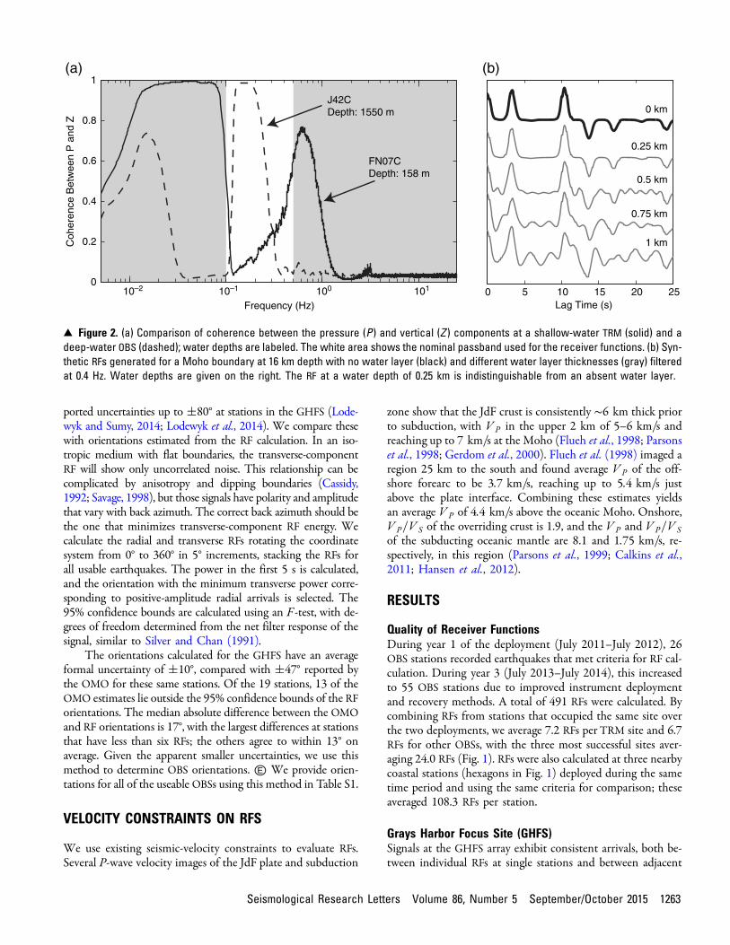
stations for lag times less than 15–20 s (Fig. 3). Hence, these RFsare dominated by coherent signal. In most cases, these signalseither do not show a zero-lag pulse representing the incidentP arrival or it is smaller than other peaks, such as typifies stationson low-velocity sediment (e.g., Sheehan et al., 1995). One of thehighest amplitude arrivals observed at every shallow-water sta-tion is a positive pulse at ∼3 s, which is observed consistentlyacross back azimuths, with variation in the timing of the pulse upto ∼1 s. Most stations show negative arrivals both before andafter this 3 s peak, similar to features observed from the onshorestationWISH, located along the GHFS–CAFE transect, for backazimuths >200° near 2 and 6 s lag (Fig. 3). This peak has beenidentified onshore as the upgoing (Ps) conversion package fromthe downgoing plate. Many of the OBS stations also have a broadnegative pulse at 12–14 s that is similar in amplitude to the peakat 3 s. In some cases, the timing (e.g., FN14) or amplitude (e.g.,FN07) of this arrival varies with back azimuth (Fig. 3). The mostsuccessful sites in terms of RF data recovery were at 150–700 m

water depths, but given the small number of stations it is notclear that depth is the main reason for the clearer signals. Thewater multiples at these depths arrive at a periodicity muchshorter than the low-pass filter frequency (Fig. 3) so should havelittle effect. At sites in<100 m of water (e.g., FN02), the signal-to-noise ratio tended to decrease, fewer RFs were recorded, andsome of the later arrivals are less visible. This is likely due to anincrease in noise from direct wave loading on the station (Webband Crawford, 2010). At FN12, the water column reverbera-tions may have a minor effect on the RFs, based on sensitivitytests (Fig. 2b).

At OBSs deployed in >1000 m of water (e.g., FN13;Fig. 3), arrivals exist that correlate between individual RFs, butthese do not match any arrivals observed at the shallow-waterstations. This may be due to a change in the structure, the ap-pearance of water column multiples, or a combination of theseeffects. The primary water column multiples should alternatepolarity, beginning with a negative arrival (Bostock and Trehu,

WISH0

5

10

15

20

25

Lag

Tim

e (s

)FN13, 1764 m FN12, 656 m FN14, 173 m FN08, 176 m FN07, 158 m FN02, 67 m

Back Azimuth Range: 0-150° Back Azimuth Range: 200-360°

▴ Figure 3. Individual radial-component RFs from six GHFS locations and the onshore site WISH for comparison. At each site, RFs are sortedin increasing back azimuth to the right; bars at the base of each station underlie individual RFs that are from particular back-azimuth ranges.Positive arrivals are indicated in black, and negative arrivals are in gray. Sites are sorted with the westernmost at the left. FN13 is a deepwater OBS, whereas others are TRM OBS; water depths are labeled. White triangles indicate times of predicted water multiples with negativepolarity, and black indicates positive polarity. A Gaussian filter with a corner frequency of 0.4 Hz has been applied to all RFs.

1264 Seismological Research Letters Volume 86, Number 5 September/October 2015

2012) at times based on the depth (Figs. 3, 4). Reverberationsgenerated by secondary phases may complicate this pattern, butthe P-coupled multiples should be much larger than those gen-erated by P-to-S conversions.

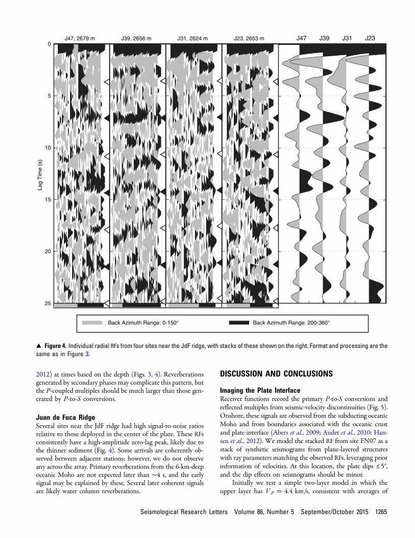
Juan de Fuca RidgeSeveral sites near the JdF ridge had high signal-to-noise ratiosrelative to those deployed in the center of the plate. These RFsconsistently have a high-amplitude zero-lag peak, likely due tothe thinner sediment (Fig. 4). Some arrivals are coherently ob-served between adjacent stations; however, we do not observeany across the array. Primary reverberations from the 6-km-deepoceanic Moho are not expected later than ∼4 s, and the earlysignal may be explained by these. Several later coherent signalsare likely water column reverberations.

DISCUSSION AND CONCLUSIONS

Imaging the Plate InterfaceReceiver functions record the primary P-to-S conversions andreflected multiples from seismic-velocity discontinuities (Fig. 5).Onshore, these signals are observed from the subducting oceanicMoho and from boundaries associated with the oceanic crustand plate interface (Abers et al., 2009; Audet et al., 2010; Han-sen et al., 2012). We model the stacked RF from site FN07 as astack of synthetic seismograms from plane-layered structureswith ray parameters matching the observed RFs, leveraging priorinformation of velocities. At this location, the plate dips ≤5°,and the dip effects on seismograms should be minor.

Initially we test a simple two-layer model in which theupper layer has VP � 4:4 km=s, consistent with averages of

J47, 2679 m J39, 2656 m J31, 2624 m J23, 2653 m0

5

10

15

20

25

Lag

Tim

e (s

)J47 J39 J31 J23

Back Azimuth Range: 0-150° Back Azimuth Range: 200-360°

▴ Figure 4. Individual radial RFs from four sites near the JdF ridge, with stacks of these shown on the right. Format and processing are thesame as in Figure 3.

Seismological Research Letters Volume 86, Number 5 September/October 2015 1265

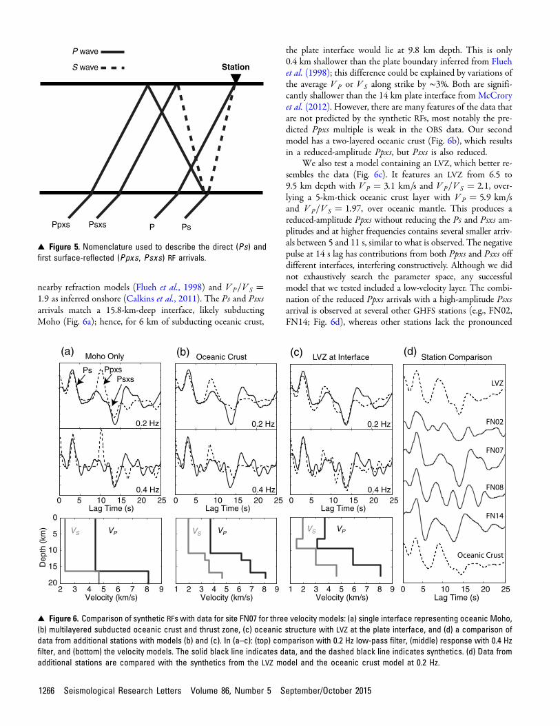
nearby refraction models (Flueh et al., 1998) and VP=V S �1:9 as inferred onshore (Calkins et al., 2011). The Ps and Psxsarrivals match a 15.8-km-deep interface, likely subductingMoho (Fig. 6a); hence, for 6 km of subducting oceanic crust,

the plate interface would lie at 9.8 km depth. This is only0.4 km shallower than the plate boundary inferred from Fluehet al. (1998); this difference could be explained by variations ofthe average VP or V S along strike by ∼3%. Both are signifi-cantly shallower than the 14 km plate interface from McCroryet al. (2012). However, there are many features of the data thatare not predicted by the synthetic RFs, most notably the pre-dicted Ppxs multiple is weak in the OBS data. Our secondmodel has a two-layered oceanic crust (Fig. 6b), which resultsin a reduced-amplitude Ppxs, but Psxs is also reduced.

We also test a model containing an LVZ, which better re-sembles the data (Fig. 6c). It features an LVZ from 6.5 to9.5 km depth with VP � 3:1 km=s and VP=V S � 2:1, over-lying a 5-km-thick oceanic crust layer with VP � 5:9 km=sand VP=V S � 1:97, over oceanic mantle. This produces areduced-amplitude Ppxs without reducing the Ps and Psxs am-plitudes and at higher frequencies contains several smaller arriv-als between 5 and 11 s, similar to what is observed. The negativepulse at 14 s lag has contributions from both Ppxs and Psxs offdifferent interfaces, interfering constructively. Although we didnot exhaustively search the parameter space, any successfulmodel that we tested included a low-velocity layer. The combi-nation of the reduced Ppxs arrivals with a high-amplitude Psxsarrival is observed at several other GHFS stations (e.g., FN02,FN14; Fig. 6d), whereas other stations lack the pronounced

P wave

S wave Station

Ppxs Psxs P Ps

▴ Figure 5. Nomenclature used to describe the direct (Ps) andfirst surface-reflected (Ppxs, Psxs) RF arrivals.

0.4 Hz 0.4 Hz 0.4 Hz0 5 10 15 20 25

Lag Time (s)0 5 10 15 20 25

Lag Time (s)

0 5 10 15 20 25Lag Time (s)

1 2 3 4 5 6 7 8 9Velocity (km/s)

0.2 Hz

Moho Only(a)

Ps PpxsPsxs

(b) Oceanic Crust

0.2 Hz

LVZ at Interface

0.2 Hz

(c) Station Comparison(d)

1 2 3 4 5 6 7 8 9Velocity (km/s)

0 5 10 15 20 25Lag Time (s)

2 3 4 5 6 7 8 9

0

5

10

15

20

VP VPVPVS VS

VS

Dep

th (

km)

Velocity (km/s)

▴ Figure 6. Comparison of synthetic RFs with data for site FN07 for three velocity models: (a) single interface representing oceanic Moho,(b) multilayered subducted oceanic crust and thrust zone, (c) oceanic structure with LVZ at the plate interface, and (d) a comparison ofdata from additional stations with models (b) and (c). In (a–c): (top) comparison with 0.2 Hz low-pass filter, (middle) response with 0.4 Hzfilter, and (bottom) the velocity models. The solid black line indicates data, and the dashed black line indicates synthetics. (d) Data fromadditional stations are compared with the synthetics from the LVZ model and the oceanic crust model at 0.2 Hz.

1266 Seismological Research Letters Volume 86, Number 5 September/October 2015

Psxs arrival (e.g., FN08; Fig. 6d). This may indicate structuralvariability; however, the similar observations at FN02, FN07,and FN14 indicate this feature may persist throughout theGHFS.

These forward models provide some indication of the ori-gin of primary features in the RFs but do not include knownvariations in velocity in the upper plate and are inherently non-unique. Effects of very low near-surface velocities (e.g., Fluehet al., 1998; Parsons et al., 1998) are evident in the lack of azero-lag pulse in the RFs but are not modeled here, so the first2 s are not well matched. The assumption of constant upper-plate velocities provides the correct timing of phases from theplate interface but will underestimate absolute velocities at thebase of the layer, thereby overestimating the velocity contrast.

Nonetheless, these models show that the RFs from OBS areimaging structures from plate-interface depths and that theLVZ likely persists offshore. Because the upper-plate velocitiesare much lower offshore than onshore where mafic Siletz ter-rane rocks probably overlie the plate boundary (Trehu et al.,

1994; Parsons et al., 1999), the persistence of the LVZ requiresvery low velocities within the offshore thrust zone. The over-riding plate has VP < 5:4 km=s, so the LVZ must have veloc-ities significantly lower and slower than nearby oceanic layer2A (Flueh et al., 1998; Gerdom et al., 2000). In addition, off-shore of Washington, the JdF crust is 6 km thick on average(Flueh et al., 1998; Gerdom et al., 2000), indicating that the 8-km-thick package of the LVZ and oceanic crust likely containssome overlying material.

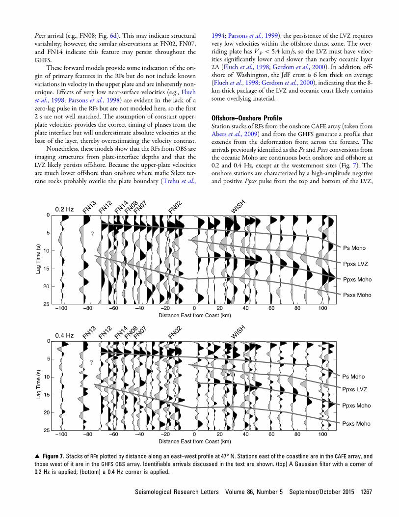
Offshore–Onshore ProfileStation stacks of RFs from the onshore CAFE array (taken fromAbers et al., 2009) and from the GHFS generate a profile thatextends from the deformation front across the forearc. Thearrivals previously identified as the Ps and Psxs conversions fromthe oceanic Moho are continuous both onshore and offshore at0.2 and 0.4 Hz, except at the westernmost sites (Fig. 7). Theonshore stations are characterized by a high-amplitude negativeand positive Ppxs pulse from the top and bottom of the LVZ,

5

Lag

Tim

e (s

)

Distance East from Coast (km)

Distance East from Coast (km)

5

Lag

Tim

e (s

)

Ps Moho

Ppxs Moho

Psxs Moho

Ppxs LVZ

?

Ps Moho

Ppxs Moho

Psxs Moho

Ppxs LVZ

?

▴ Figure 7. Stacks of RFs plotted by distance along an east–west profile at 47° N. Stations east of the coastline are in the CAFE array, andthose west of it are in the GHFS OBS array. Identifiable arrivals discussed in the text are shown. (top) A Gaussian filter with a corner of0.2 Hz is applied; (bottom) a 0.4 Hz corner is applied.

Seismological Research Letters Volume 86, Number 5 September/October 2015 1267

respectively. These arrivals are not clearly observed on the OBS,whereas the later-arriving Psxs is clearer.

Results from forward modeling indicate these features arebest explained by a velocity inversion at the plate interface us-ing a shallower and slower structure than is observed onshore.The base of the overriding crust beneath the GHFS is expectedto have VP � 5:0–5:4 km=s (Flueh et al., 1998; Parsons et al.,1999). Because modeling indicates a decrease of ∼0:5 km=s inVP at the plate interface using the VP=V S constraints describedabove, the LVZ beneath FN07 likely has VP � 4:5–4:9 km=s,which is slightly slower than the 5:0� 0:3 km=s observedonshore (Abers et al., 2009). Similar observations of reducedvelocities have been reported in the Nankai subduction zone ap-proximately 10 km below sea floor (Kamei et al., 2012), similarto plate-interface depths observed in our study, and were inter-preted as high-porosity underthrust sediment (Bangs et al.,2009). In addition, anisotropy could contribute to velocity re-duction in the interplate shear zone, but we do not investigatethis further. Nedimovic et al. (2003) observed an abrupt changein reflectivity moving up-dip offshore Vancouver Island, whichmight be manifest here as structural changes beneath the stationsclosest to the deformation front. However, structures within5 km of the surface are hard to observe with RFs.

In summary, RFs can be calculated using data from OBS inforearc settings. The shielded TRM OBS exhibit low noise in thecritical 0.1–0.4 Hz band, particularly on horizontal components.The offshore RFs from the GHFS record arrivals from a structureassociated with the subducting oceanic crust, allowing continu-ous imaging of the plate interface nearly to the deformationfront. Forward modeling indicates the subducting Moho is∼16 km deep at FN07, located ∼45 km offshore of Grays Har-bor; the precise depth depends on the overlying structure. For-ward modeling also suggests that an LVZ at the zplate interfacecan explain several of the features observed in the RFs at this site,indicating that this structure may persist into the locked zone.

ACKNOWLEDGMENTS

This work is funded by National Science Foundation AwardNumbers OCE-1334831 and EAR-1147622 and is based uponwork supported by the National Science Foundation GraduateResearch Fellowship under Grant Number DGE-11-44155.The offshore data used in this research were provided by in-struments from the Ocean-Bottom Seismograph (OBS) Instru-ment Pool (http://www.obsip.org; last accessed November2014), and the onland data are part of the EarthScope facility,both part of the Cascadia Initiative Amphibious Array fundedby the National Science Foundation. All the seismic data arearchived at the Incorporated Research Institutions for Seismol-ogy (IRIS) Data Management Center (http://www.iris.edu). Wethank Spahr Webb for providing valuable insight into under-standing the noise properties of the OBS instruments and KatieKeranen and Dana Peterson for providing stacking velocitiesfrom the Cascadia Open-Access Seismic Transects (COAST)cruise. This work benefitted from constructive reviews by PascalAudet and an anonymous reviewer.

REFERENCES

Abers, G. A., L. S. MacKenzie, S. Rondenay, Z. Zhang, A. G. Wech, andK. C. Creager (2009). Imaging the source region of Cascadia tremorand intermediate-depth earthquakes, Geology 37, no. 12, 1119–1122.

Audet, P., M. G. Bostock, D. C. Boyarko, M. R. Brudzinski, and R. M.Allen (2010). Slab morphology in the Cascadia fore arc and its re-lation to episodic tremor and slip, J. Geophys. Res. 115, no. B00A16,doi: 10.1029/2008JB006053.

Audet, P., M. G. Bostock, N. I. Christensen, and S. M. Peacock (2009).Seismic evidence for overpressured subducted oceanic crust andmegathrust fault sealing, Nature 457, no. 7225, 76–77.

Ball, J. S., A. F. Sheehan, J. C. Stachnik, F.-C. Lin, and J. A. Collins(2014). A joint Monte Carlo analysis of seafloor compliance, Ray-leigh wave dispersion and receiver functions at ocean bottom seismicstations offshore New Zealand, Geochem. Geophys. Geosyst. 15, doi:10.1002/2014GC005412.

Bangs, N. L. B., G. F. Moore, S. P. S. Gulick, E. M. Pangborn, H. J. Tobin,S. Kuramoto, and A. Taira (2009). Broad, weak regions of theNankai megathrust and implications for shallow coseismic slip,Earth Planet. Sci. Lett. 284, 44–49.

Bell, S. W., D. W. Forsyth, and Y. Ruan (2014). Removing noise from thevertical component records of ocean-bottom seismometers: Resultsfrom year one of the Cascadia Initiative, Bull. Seismol. Soc. Am. 105,no. 1, doi: 10.1785/0120140054.

Bostock, M. G., and A. M. Trehu (2012). Wave-field decomposition ofocean bottom seismograms, Bull. Seismol. Soc. Am. 102, no. 4,1681–1692.

Brillon, C., J. F. Cassidy, and S. E. Dosso (2013). Onshore/offshore struc-ture of the Juan de Fuca plate in northern Cascadia from Bayesianreceiver function inversion, Bull. Seismol. Soc. Am. 103, no. 5,2914–2920.

Calkins, J. A., G. A. Abers, G. Ekstrom, K. C. Creager, and S. Rondenay(2011). Shallow structure of the Cascadia subduction zone beneathwesternWashington from spectral ambient noise correlation, J. Geo-phys. Res. 116, no. B07302, doi: 10.1029/2010JB007657.

Cassidy, J. F. (1992). Numerical experiments in broadband receiver func-tion analysis, Bull. Seismol. Soc. Am. 82, 1453–1474.

Cozzens, B. D., and G. A. Spinelli (2012). A wider seismogenic zone atCascadia due to fluid circulation in subducting oceanic crust, Geol-ogy 40, no. 10, 899–902.

Crawford,W. C., and S. C. Webb (2000). Removing tilt noise from lowfrequency (<0:1 Hz) seafloor vertical seismic data, Bull. Seismol.Soc. Am. 90, no. 4, 952–963.

DeMets, C., R. G. Gordon, D. F. Argus, and S. Stein (1994). Effect ofrecent revisions to the geomagnetic reversal time scale on estimatesof current plate motions, Geophys. Res. Lett. 21, 2191–2194.

Flueh, E. R., M. A. Fisher, J. Bialas, J. R. Childs, D. Klaeschen, N. Ku-kowski, T. Parsons, D. W. Scholl, U. ten Brink, A. M. Trehu, and N.Vidal (1998). New seismic images of the Cascadia subduction zonefrom cruise SO108—ORWELL, Tectonophysics 293, 69–84.

Gerdom, M., A. M. Trehu, E. R. Flueh, and D. Klaeschen (2000). Thecontinental margin off Oregon from seismic investigations, Tecto-nophysics 329, 79–97.

Goldfinger, C., C. H. Nelson, and J. E. Johnson (2003). Deep-water tur-bidites as Holocene earthquake proxies: The Cascadia subductionzone and northern San Andreas fault systems, Annu. Rev. EarthPlanet. Sci. 46, 1169–1194.

Hacker, B. R., G. A. Abers, and S. M. Peacock (2003). Subduction factory,1, theoretical mineralogy, densities, seismic wave speeds, andH2O con-tents, J. Geophys. Res. 108, no. B1, 2029, doi: 10.1029/2001JB001127.

Hansen, R. T. J., M. G. Bostock, and N. I. Christensen (2012). Nature ofthe low velocity zone in Cascadia from receiver function waveforminversion, Earth Planet. Sci. Lett. 337/338, 25–38.

Hyndman, R. D., and K. Wang (1993). Thermal constraints on the zoneof major thrust earthquake failure: The Cascadia subduction zone, J.Geophys. Res. 98, no. B2, 2039–2060.

1268 Seismological Research Letters Volume 86, Number 5 September/October 2015

Kamei, R., R. G. Pratt, and T. Tsuji (2012). Waveform tomographyimaging of a megasplay fault system in the seismogenic Nankai sub-duction zone, Earth Planet. Sci. Lett. 317/318, 343–353.

Leahy, G. M., J. A. Collins, C. J. Wolfe, G. Laske, and S. C. Solomon(2010). Underplating of the Hawaiian swell: Evidence from teleseis-mic receiver functions, Geophys. J. Int. 183, 313–329.

Ligorria, J. P., and C. J. Ammon (1999). Iterative deconvolution and receiver-function estimation, Bull. Seismol. Soc. Am. 89, no. 5, 1395–1400.

Liu, Y., and J. R. Rice (2007). Spontaneous and triggered aseismic defor-mation transients in a subduction fault model, J. Geophys. Res. 112,no. B09404, doi: 10.1029/2007JB004930.

Lodewyk, J., and D. Sumy (2014). Cascadia Amphibious Array Ocean Bot-tom Seismograph Horizontal Component Orientations, 2013-2014OBS Deployments, OBSIP Management Office Incorporated Re-search Institutions for Seismology.

Lodewyk, J., A. Frassetto, A. Adinolfi, and B. Woodward (2014).Cascadia Amphibious Array Ocean Bottom Seismograph HorizontalComponent Orientations, 2011-2012 OBS Deployments, Version 3.0,OBSIP Management Office Incorporated Research Institutions forSeismology.

McCaffrey, R., R. W. King, S. J. Payne, and M. Lancaster (2013). Activetectonics of northwestern U.S. inferred from GPS-derived surfacevelocities, J. Geophys. Res. 118, 1–15.

McCrory, P. A., J. L. Blair, F. Waldhauser, and D. H. Oppenheimer(2012). Juan de Fuca slab geometry and its relation to Wadati–Benioff zone seismicity, J. Geophys. Res. 117, no. B09306, doi:10.1029/2012JB009407.

Nedimovic, M. R., R. D. Hyndman, K. Ramachandran, and G. D. Spence(2003). Reflection signature of seismic and aseismic slip on thenorthern Cascadia subduction interface, Nature 424, 416–420.

Nelson, A. R., B. F. Atwater, T. Bobrowsky, L.-A. Bradley, J. J. Clague, G.A. Carver, M. E. Darienzo,W. C. Grant, H. W. Krueger, R. Sparks,T. W. Stafford Jr., and M. Stuiver (1995). Radiocarbon evidence forextensive plate-boundary rupture about 300 years ago at the Casca-dia subduction zone, Nature 378, 371–374.

Nicholson, T., M. Bostock, and J. F. Cassidy (2005). New constraints onsubduction zone structure in northern Cascadia, Geophys. J. Int.161, 849–859.

Oleskevich, D. A., R. D. Hyndman, and K. Wang (1999). The updip anddowndip limits to great subduction earthquakes: Thermal and struc-tural models of Cascadia, south Alaska, SW Japan, and Chile,J. Geophys. Res. 104, no. B7, 14,965–14,991.

Parsons, T., A. M. Trehu, J. H. Luetgert, K. Miller, F. Kilbride, R. E.Wells, M. A. Fisher, E. Flueh, U. S. ten Brink, and N. I. Christensen(1998). A new view into the Cascadia subduction zone and volcanicarc: Implications for earthquake hazards along theWashington mar-gin, Geology 26, no. 3, 199–202.

Parsons, T., R. E. Wells, M. A. Fisher, E. Fleuh, and U. S. ten Brink(1999). Three-dimensional velocity structure of Siletzia and otheraccreted terranes in the Cascadia forearc of Washington, J. Geophys.Res. 104, no. B8, 18,015–18,039.

Rondenay, S., M. G. Bostock, and J. Shragge (2001). Multiparametertwo-dimensional inversion of scattered teleseismic body waves, 3:Application to the Cascadia 1993 data set, J. Geophys. Res. 106,30,795–30,808.

Saffer, D. M., and H. Tobin (2011). Hydrogeology and mechanics ofsubduction zone forearcs: Fluid flow and pore pressure, Annu.Rev. Earth Planet. Sci. 39, 157–186.

Savage, M. K. (1998). Lower crustal anisotropy or dipping boundary?Effects on receiver functions and a case study in New Zealand,J. Geophys. Res. 103, no. 7, 15,069–15,087.

Sheehan, A. F., G. A. Abers, C. H. Jones, and A. L. Lerner-Lam (1995).Crustal thickness variations across the Colorado RockyMountains fromteleseismic receiver functions, J. Geophys. Res. 100, 20,391–20,404.

Silver, P. G., and W. W. Chan (1991). Shear wave splitting and subcontinen-tal mantle deformation, J. Geophys. Res. 96, no. B10, 16,429–16,454.

Stachnik, J. C., A. F. Sheehan, D. W. Zietlow, Z. Yang, J. Collins, and A.Ferris (2012). Determination of New Zealand ocean bottom seis-mometer orientation via Rayleigh-wave polarization, Seismol. Res.Lett. 83, 704–712.

Toomey, D. R., R. M. Allen, A. H. Barclay, S. W. Bell, P. D. Bromirski,R. L. Carlson, X. Chen, J. A. Collins, R. P. Dziak, B. Evers, et al.(2014). The Cascadia Initiative: A sea change in seismological stud-ies of subduction zones, Oceanography 27, no. 2, 138–150.

Trehu, A. M., I. Asudeh, T. M. Brocher, J. H. Luetgert, W. D. Mooney,J. L. Nabelek, and Y. Nakamura (1994). Crustal architecture of theCascadia forearc, Science 266, no. 5183, 237–243.

Webb, S. C., and W. C. Crawford (2010). Shallow-water broadbandOBS seismology, Bull. Seismol. Soc. Am. 100, 4, 1770–1778

Webb, S. C., A. H. Barclay, D. Gassier, and T. Koczynski (2013). Seismicobservations in shallow water, presented at 2013 Fall Meeting, AGU,San Francisco, California, 9–13 December, Abstract S12A-02.

Helen A. JaniszewskiDepartment of Earth and Environmental Sciences

Lamont Doherty Earth Observatory of Columbia University61 Route 9W

Palisades, New York 10964 U.S.A.helenj@ldeo.columbia.edu

Geoffrey A. AbersDepartment of Earth and Atmospheric Sciences

Cornell University4126 Snee Hall

Ithaca, New York 14853 U.S.A.

Published Online 19 August 2015

Seismological Research Letters Volume 86, Number 5 September/October 2015 1269