E-matching for Fun and Profit

Micha!l Moskal∗

Jakub !Lopuszanski

University of Wroc!law, Poland

Joseph R. Kiniry

University College Dublin, Ireland

Abstract

Efficient handling of quantifiers is crucial for solving software verification problems.

E-matching algorithms are used in satisfability modulo theories solvers that handle

quantified formulas through instantiation. Two novel, efficient algorithms for solv-

ing the E-matching problem are presented and compared to a well-known algorithm

described in the literature.

1 Motivation

Satisfability Modulo Theories (SMT) checkers usually operate in the quantifier-free frag-

ments of their respective logics. Yet program verification problems often require expres-

siveness and flexibility in extending the underlying background theories with universally

quantified axioms. The typical solution to this problem is to generate ground instances

of the quantified subformulas during the course of the proof search and hope that the

particular instances generated are the ones required to prove unsatisfiability.

As an example, consider the formula, which we try to satisfy modulo linear arithmetic

and uninterpreted function symbols theories:

P (f(42)) ∧ ∀x. P (f(x)) ⇒ x < 0∗Partially supported by Polish Ministry of Science and Education grant 3 T11C 042 30.

1

If the prover were able to guess the implication:

(∀x. P (f(x)) ⇒ x < 0) ⇒ P (f(42)) ⇒ 42 < 0

then, by boolean unit resolution (with the currently known facts P (f(42)) and ∀x. P (f(x)) ⇒

x < 0) the prover would try to assert 42 < 0, which would cause contradiction in the linear

arithmetic decision procedure.

The tricky part is how to figure out which instances are going to be useful. A well-

known [6] solution is to designate subterms occurring in the quantified formula called

triggers, and only add instances that make those subterms equal to ground subterms that

are currently being considered in the proof. In our example one such trigger is P (f(x)),

which works as expected.

However it is often not enough to consider only syntactic equality. If we modify our

example a little bit:

a = f(42) ∧ P (a) ∧ ∀x. P (f(x)) ⇒ x < 0

our choice of trigger no longer works. We could use a less restrictive trigger (namely f(x)),

but it leads to generating excessive, irrelevant instances, which reduces the efficiency of

the prover. We therefore use a different technique: instead of using syntactic equality, use

the equality relation induced by the current context. For example: in the context P (a),

a = f(42) the substitution [x := 42] makes the term P (f(x)) equal to P (a).

Because we do not consider boolean formulas terms, it is sometimes not possible to

designate a single trigger containing all the variables that are quantified. A classical

example is the transitivity axiom. In such a case we use a multitrigger, which is a set of

triggers, hopefully sharing variables, that are supposed to match simultaneously.

There are two remaining problems here: identifying the set of triggers for a given

formula, and identifying the substitutions that make the trigger equal to some ground

term. As for the first problem, it is possible to apply heuristics1, as well as ask the user,

to provide the triggers. The second problem is E-matching. We present a well-known1Some heuristics are described in the Simplify technical report [6].

2

algorithm for solving it (Sect. 3), introduce two other, efficient algorithms (Sect. 4 and 5)

and compare them to the well-known one.

2 Definitions

Let V be the infinite, enumerable set of variables. Let Σ be the set of function and constant

symbols. Let T be the set of first order terms constructed over Σ and V.

A substitution is a function σ : V → T that is not identity for a finite number of

parameters. We identify a substitution with its homomorphic extension to all terms (i.e.,

σ : T → T ). Let S be the set of all substitutions.

We will use letters x and y, possibly with indices for variables, f and g for function

symbols, c and d for constant symbols (functions of arity zero), σ and ρ for substitutions,

t for ground terms, and p for possibly non-ground terms. We will use the notation [x1 :=

t1, . . . , xn := tn] for substitutions, and σ[x := t] for a substitution augmented to return t

for x.

An instance of an E-matching problem2 consists of a finite set of active ground terms

A ⊆ T , a relation ∼=g ⊆ A × A, and a finite set of non-variable, non-constant terms

p1, . . . , pn, which we call the triggers. Let ∼= ⊆ T × T be the smallest congruence relation

containing ∼=g. Let root : T → T be a function3 such that:

(∀t, s ∈ T . root(t) = root(s) ⇔ t ∼= s) ∧ (∀t ∈ T . root(t) ∼= t)

The solution to the E-matching problem is the set:

T =

σ

∣∣∣∣∣∣∣

∃t1, . . . , tn ∈ A.σ(p1) ∼= t1 ∧ . . . ∧ σ(pn) ∼= tn,

∀x ∈ V.σ(x) = root(σ(x))

The problem of deciding for a fixed A and ∼=g, and a given trigger, if T += ∅, is NP-

hard [10]. The NP-hardness is why each solution to the problem is inherently backtracking2In automated reasoning literature, the term E-matching usually refers to a slightly different problem,

where A is a singleton and ∼= is not restricted to be finitely generated. On the other hand the Simplifytechnical report [6] as well as the recent Z3 paper [5] use the term E-matching in the sense defined above.

3Such a function exists by virtue of ∼= being equivalence relation, and is provided by the typical datastructure used to represent ∼=, namely the E-graph (see Simplify technical report [6] for details on E-graph).

3

fun simplify match([p1, . . . , pn])R := ∅proc match(σ, j)

if j = nil then R := R ∪ {σ}else case hd(j) of

(c, t) ⇒ /∗ 1 ∗/if c ∼= t then match(σ, tl(j))else skip

(x, t) ⇒ /∗ 2 ∗/if σ(x) = x then match(σ[x := root(t)], tl(j))else if σ(x) = root(t) then match(σ, tl(j))else skip

(f(p1, . . . , pn), t) ⇒ /∗ 3 ∗/foreach f(t1, . . . , tn) in A do

if t = ∗ ∨ root(f(t1, . . . , tn)) = t thenmatch(σ, (p1, root(t1)) :: . . . :: (pn, root(tn)) :: tl(j))

match([], (p1, ∗) :: . . . :: (pn, ∗) :: nil) /∗ 4 ∗/return R

Figure 1: Simplify’s matching algorithm

in nature. In practice, though, the triggers that are used are small, and the problem is

not the complexity of a backtracking search for a particular trigger, but rather the fact

that in a given proof search there are often hundreds of thousands of matching problems

to solve.

3 Simplify’s Matching Algorithm

The Simplify technical report [6] describes a recursive matching algorithm simplify match

given in Fig. 1. The symbol :: denotes a list constructor, nil is an empty list and [] is an

empty (identity) substitution. hd and tl are the functions returning, respectively, head

and tail of a list (i.e., hd(x :: y) = x and tl(x :: y) = y). The command skip is a no-op.

The simplify match algorithm maintains the current substitution and a stack (imple-

mented as a list) of (trigger, ground term) pairs to be matched. We refer to these pairs

as jobs. Additionally, it uses the special symbol ∗ in place of a ground term to say that

we are not interested in matching against any specific term, as any active term will do.

We start (line marked /∗ 4 ∗/) by putting the set of triggers to be matched on the stack

and then proceed by taking the top element of the stack.

If the trigger in the top element is a constant (/∗ 1 ∗/), we just compare it against the

4

ground term, and if the comparison succeeded, recurse.

If the trigger is a variable x (/∗ 2 ∗/), we check if the current substitution already

assigns some value to that variable, and if so, we just compare it against the ground term

t. Otherwise we extend the current substitution by mapping x to t and recurse. Observe

that t cannot be ∗, because we do not allow triggers to be single variables.

If the trigger is a complex term f(p1, . . . , pn) (/∗ 3 ∗/), we iterate over all the terms

with f in the head (possibly checking if they are equivalent to the ground term we are

supposed to match against), construct the set of jobs matching respective children of the

trigger against respective children of the ground term, and recurse.

The important invariants of simplify match are: (1) the jobs lists contain stars instead

of ground terms only for non-variable, non-constant triggers; (2) all the ground terms t in

the job lists satisfy root(t) = t.

The detailed discussion of this procedure is given in the Simplify technical report [6].

4 Subtrigger Matcher

This section describes a novel matching algorithm, optimized for linear triggers. A lin-

ear trigger is a trigger in which each variable occurs at most once. Most triggers used

in program verification problems we have inspected are linear. The linearity means that

matching problems for subterms of a trigger are independent, which allows for more effi-

cient processing.

However, even if triggers are not linear, it pays off to treat them as linear, and only

after the matching algorithm is complete discard the resulting substitutions that assign

different terms to the same variable. This technique is often used in term indexes [12]

used in automated reasoning. The algorithm, therefore, does not require the trigger to be

linear.

This matcher algorithm is given in Fig. 2. It uses operations 0 and 1, which are defined

on sets of substitutions:

5

fun fetch(S, t, p)if S = 2 then return {[p := root(t)]}else if S = × ∧ t ∼= p then return {[]}else if S = × then return ∅else return S(root(t))

fun match(p)case p of

x ⇒ return 2c ⇒ return ×f(p1, . . . , pn) ⇒

foreach i in 1 . . . n do Si = match(pi) /∗ 1 ∗/if ∃i. Si = ⊥ then return ⊥ /∗ 2 ∗/if ∀i. Si = × then return × /∗ 3 ∗/S := {t 4→ ∅ | t ∈ A}foreach f(t1, . . . , tn) in A do /∗ 4 ∗/

t := root(f(t1, . . . , tn))S := S[t 4→ S(t) 1 (fetch(S1, t1, p1) 0 . . . 0 fetch(Sn, tn, pn))]

if ∀t. S(t) = ⊥ then return ⊥else return S

fun topmatch(p) /∗ 5 ∗/S := match(p)return

⊔t∈A S(t)

fun subtrigger match([p1, . . . , pn])return topmatch(p1) 0 . . . 0 topmatch(pn)

Figure 2: Subtrigger matching algorithm

A 0B = {σ ⊕ ρ | σ ∈ A, ρ ∈ B,σ ⊕ ρ += ⊥}

A 1B = A ∪B

σ ⊕ ρ =

⊥ when ∃x.σ(x) += x ∧ ρ(x) += x ∧ σ(x) += ρ(x)

σ · ρ otherwise

σ · ρ(x) =

σ(x) when σ(x) += x

ρ(x) otherwise

0 returns a set of all possible non-conflicting combinations of two sets of substitutions. 1

sums two such sets. The next section shows an implementation of these operations that

does not use explicit sets.

The match(p) function returns the set of all substitutions σ, such that σ(p) ∼= t, for a

term t ∈ A, categorized by root(t). More specifically, match returns a map from root(t)

6

to such substitutions, or one of the special symbols 2, ⊥, ×. Symbol 2 means that p was

a variable x, and therefore the map is: {t 4→ {[x := t]} | t ∈ A, root(t) = t}, symbol ⊥

represents no matches (i.e., {t 4→ ∅ | t ∈ A}), and × means p was ground, so the map is

{root(p) 4→ {[]}} ∪ {t 4→ ∅ | t ∈ A, t += root(p)}4.

The only non-trivial control flow case in the match function is the case of a complex

trigger f(p1, . . . , pn), which works as follows:

• /∗ 1 ∗/ recurse on subtriggers. Conceptually, we consider the subtriggers to be inde-

pendent of each other (i.e., f(p1, . . . , pn) is linear). If they are, however, dependant,

then the 0 operation filters out conflicting substitutions.

• /∗ 2 ∗/ check if there is any subtrigger that does not match anything, in which case

the entire trigger does not match anything.

• /∗ 3 ∗/ check if all our children are ground, in which case we are ground as well.

• /∗ 4 ∗/ otherwise we start with an empty result map S and iterate over all terms with

the correct head symbol. For each such term f(t1, . . . , tn), we combine (using 1) the

already present results for root(f(t1, . . . , tn)) with results of matching pi against ti.

The fetch function is used to retrieve results of subtrigger matching by ensuring the

special symbols are treated as the maps they represent.

Finally (/∗ 5 ∗/) the topmatch function just collapses the maps into one big set.

4.1 S-Trees

The idea behind s-trees is to have a compact representation of sets of substitutions that

are efficiently manipulated during the matching.

The s-trees data structure itself can be viewed as a special case of substitution trees

used in the automated reasoning [12], with rather severe restrictions on their shape. We,

however, do not use the trees as an index and, in consequence, require a different set of

operations.4Here we assume all the ground subterms of triggers to be in A. This is easily achieved and does not

affect performance in our tests.

7

Figure 3: Example of s-tree operations

S-trees require a strict, total order ≺ ⊆ A × A and are defined inductively: (1) ε is

an s-tree; (2) if T1, . . . , Tn are s-trees and t1, . . . , tn are ground terms, then x ! ((t1, T1) ::

. . . :: (tn, Tn) :: nil) is an s-tree.

The invariant of the data structure is that in each node i < j ⇒ ti ≺ tj , and that

there exists a sequence of variables x1 . . . xk such that the root is x1 ! (. . .) and each

node (including the root) is xi ! ((t1, xi+1 ! (. . .)) :: . . . :: (tn, xi+1 ! (. . .)) :: nil) or

xk ! ((t1, ε) :: . . . :: (tn, ε) :: nil) for some n, t1, . . . , tn and 1 ≤ i < k. In other words, the

variables at a given level of a tree are the same.

The yield function maps a s-tree into the set of substitutions it is intended to represent.

yield(ε) = {[]}

yield(x ! ((t1, T1) :: . . . :: (tn, Tn) :: nil)) =

σ[x := ti]

∣∣∣∣∣∣∣∣∣∣

i ∈ {1, . . . , n},

σ ∈ yield(Ti)

σ(x) = x ∨ σ(x) = ti

Example s-trees are given in Fig. 3. The trees are represented as ordered directed

acyclic graphs with aggressive sharing. An s-tree x ! ((t1, T1) :: . . . :: (tn, Tn) :: nil) has

the label x on the node, ti label the edges and each edge leads to another tree Ti. The

8

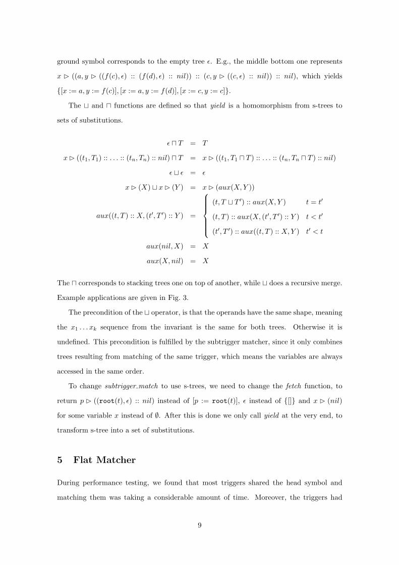
ground symbol corresponds to the empty tree ε. E.g., the middle bottom one represents

x ! ((a, y ! ((f(c), ε) :: (f(d), ε) :: nil)) :: (c, y ! ((c, ε) :: nil)) :: nil), which yields

{[x := a, y := f(c)], [x := a, y := f(d)], [x := c, y := c]}.

The 1 and 0 functions are defined so that yield is a homomorphism from s-trees to

sets of substitutions.

ε 0 T = T

x ! ((t1, T1) :: . . . :: (tn, Tn) :: nil) 0 T = x ! ((t1, T1 0 T ) :: . . . :: (tn, Tn 0 T ) :: nil)

ε 1 ε = ε

x ! (X) 1 x ! (Y ) = x ! (aux(X, Y ))

aux((t, T ) :: X, (t′, T ′) :: Y ) =

(t, T 1 T ′) :: aux(X, Y ) t = t′

(t, T ) :: aux(X, (t′, T ′) :: Y ) t < t′

(t′, T ′) :: aux((t, T ) :: X, Y ) t′ < t

aux(nil,X) = X

aux(X, nil) = X

The 0 corresponds to stacking trees one on top of another, while 1 does a recursive merge.

Example applications are given in Fig. 3.

The precondition of the 1 operator, is that the operands have the same shape, meaning

the x1 . . . xk sequence from the invariant is the same for both trees. Otherwise it is

undefined. This precondition is fulfilled by the subtrigger matcher, since it only combines

trees resulting from matching of the same trigger, which means the variables are always

accessed in the same order.

To change subtrigger match to use s-trees, we need to change the fetch function, to

return p ! ((root(t), ε) :: nil) instead of [p := root(t)], ε instead of {[]} and x ! (nil)

for some variable x instead of ∅. After this is done we only call yield at the very end, to

transform s-tree into a set of substitutions.

5 Flat Matcher

During performance testing, we found that most triggers shared the head symbol and

matching them was taking a considerable amount of time. Moreover, the triggers had

9

Figure 4: Example of an index for flat triggers with g in head

a very simple form: f(x, c)5. This form is a specific example of something we call flat

triggers. A flat trigger is a trigger in which each variable occurs at most once and at the

depth of one.

Flat triggers with a given head can be matched all at once, by constructing a tree that

indexes all the triggers with given function symbol in the head. Such a tree can be viewed

as a special kind of a discrimination tree [12], where we consider each child of the pattern

as a constant term, instead of traversing it pre-order.

We assume, without loss of generality, each function symbol to have only one ar-

ity. A node in the index tree is either a set of triggers {p1, . . . , pn}, or a set of pairs

{(t1, I1), . . . , (tn, In)} where each of the ti is a ground term or a special symbol ∗, and Ii

are index trees.

We call (t1, . . . , tn, p) a path in I if and only if: (1) n = 0 and p ∈ I; or (2) (t1, I ′) ∈ I

and (t2, . . . , tn, p) is a path in I ′.

Let star(x) = ∗ for a variable x and star(t) = t, for any non-variable term t. We

say that I indexes a set of triggers Q if for any f(p1, . . . , pn) ∈ Q there exists a path

(star(p1), . . . , star(pn), f(p1, . . . , pn)) in I, and for every path there exists a corresponding

trigger.

Given an index I, we find all the triggers that match the term f(t1, . . . , tn) by calling

match′(f(t1, . . . , tn), (t1, . . . , tn), {I}), where match′ is defined as follows:

match′(t, (t1, . . . , tn), A) =

match′(t, (t2, . . . , tn), {I ′ | I ∈ A, (p, I ′) ∈ I, p ∼= t1 ∨ p = ∗})

match′(f(t1, . . . , tn), nil, A) =

{f(p1, . . . , pn) 4→ 0i=1...n, pi∈V [pi := root(ti)] | I ∈ A, f(p1, . . . , pn) ∈ I}

5The actual function symbol was the subtyping predicate.

10

fun topmatch(p)if p is flat then

let f(p1, ..., pn) = pIf := index for all triggers with head fforeach p in If do Sp := ∅foreach f(t1, . . . , tn) in A do

foreach t 4→ T in match′(f(t1, . . . , tn), [t1, . . . , tn], If ) doSt := St 1 T

return Sp

elseS := match(p)return

⊔t∈A S(t)

Figure 5: Flat matcher

The algorithm works by maintaining the set of trigger indices A containing triggers that

still possibly match t. At the bottom of the tree we extract the children of t corresponding

to variables in the trigger, skipping over ground subterms of the trigger.

A flat-aware matcher is implemented by replacing the topmatch function from Fig. 2

with the one from Fig. 5. The point of using it, though, is to cache If and St across calls

to subtrigger match.

6 Implementation and Experiments

We have implemented all three algorithms inside the Fx7 SMT checker6. Fx7 is imple-

mented in the Nemerle language and runs on the .NET platform. In each case the im-

plementation is highly optimized and only unsatisfactory results with the simplify match

algorithm led to designing and implementing second and third algorithm.

The implementation makes heavy use of memoization. Both terms and s-trees use

aggressive (maximal) sharing. The implementations of 0 and 1 memoize results. We also

use subtraction operation on s-trees, corresponding to set subtraction. Its implementation

looks very much like 1.

An important point to consider in the design of matching algorithms is incrementality.

The prover will typically match, assert a few facts, and then match again. The prover is

then interested only in receiving the new results. The Simplify technical report [6] cites6Available online at http://nemerle.org/fx7/.

11

two optimizations to deal with incrementality. We have implemented one of them, the

mod-time optimization, in all three algorithms. The effects are mixed, mainly because our

usage patterns of the matching algorithm are different than those of Simplify: we generally

change the E-graph more between matchings due to our proof search strategy.

To achieve incrementality we memoize s-trees returned on a given proof path and then

use the subtraction operation to remove substitutions that had been returned previously.

Another fine point is that the loop over all active terms in the implementations of

all three algorithms skips some terms: if we have inspected f(t1, . . . , tn) then we skip

f(t′1, . . . , t′n) given that ti ∼= t′i for i = 1 . . . n. Following work on fast, proof-producing

congruence closure [11], we encode all the terms using only constants and a single bi-

nary function symbol ·(. . .). E.g., f(t1, . . . , tn) is represented by ·(f, ·(t1, . . . · (tn−1, tn))).

Therefore the loop over active terms is skipped when root(·(t1, . . .·(tn−1, tn))) was already

visited.

We use a representation of terms, where only constants and a single binary function

symbol (this is due to the fast, proof-producing congruence closure If the term represen-

tation used is based on a single binary function symbol and constants, it is easy to spot

such cases.

Yet another issue is that we map all the variables to one special symbol during the

matching, do not store the variable names in s-trees, and only introduce the names when

iterating the trees to get the final results (inside the yield function). This allows for more

sharing of subtriggers between different triggers.

The test were performed on a 1 GHz Pentium III box with 512 MiB of RAM running

Linux and Nemerle r7446 on top of Mono 1.2.3. The memory used was always under 200

MiB. We run the prover on a set of verification queries generated by the ESC/Java [9] and

Boogie [2] tools. The benchmarks are now available as part of the SMT-LIB [13].

The flat matcher helps speed up matching by around 20% in the Boogie benchmarks

and around 50% in the ESC/Java benchmarks. The flat matcher is around 2 times faster

than Simplify’s matcher in the Boogie benchmarks and around 10 times in the ESC/Java

benchmarks.

Now we give some intuitions behind the results. For example, consider the trigger

f(g1(x1), . . . , gn(xn)). If each of gi(xi) returns two matches, except for the last one, that

12

does not match anything, the subtrigger matcher exits after O(n) steps, while the simplify

matcher does O(2n) steps. Even when gn(xn) actually matches something (which is more

common), the subtrigger algorithm still does O(n) steps to construct the s-tree and only

does O(2n) steps walking that tree. These steps are much cheaper (the tree is rather small

and fits the CPU cache) than matching g2, g3 and so on several times, which Simplify’s

algorithm does. The main point of the subtrigger matcher is therefore not to repeat work

for a given (sub)trigger more than once.

The benefits of the flat matcher seem to be mostly CPU cache related. Given that we

have 100 triggers with head f and 1000 ground terms with the head f , the flat matcher

processes 1000 times a data structure of size 100, while the subtrigger matcher (and also

Simplify’s matcher) processes 100 times data structure of size 1000. Consequently, given

the data structures take considerable amounts of memory, 100 fits the cache and 1000 does

not.

7 Conclusions and Related Work

We have presented two novel algorithms for E-matching. They are shown to outperform

the well-known Simplify E-matching algorithm.

The problem was first described, along with a solution, in the Simplify technical re-

port [6]. We know several SMT checkers, like Zap [1], CVC3 [3], Verifun [8], Yices [7] and

Ergo [4] include matching algorithms, though there seem to be no publications describing

it. Specifically Zap uses a different algorithm that also relies on the fact of triggers being

linear and uses a different kind of s-trees. It however does not do anything special about

flat triggers.

In a recent paper [5] on Z3 (a rewrite of the Zap prover) the authors define a way of

compiling patterns into a code tree that is later executed against ground terms. Such a

tree brings benefits if there is many triggers that share top-part. We exploit sharing in

the bottom parts of triggers, and the flat matcher handles the case of simple triggers that

share only the head symbol. Z3 authors also propose an index on the ground terms used to

speed up matching in an incremental usage pattern. Such a index could be perhaps used

also with our approach. Usefulness of all those techniques largely depends on benchmarks

13

and the particular search strategy employed in an SMT solver.

Some of the problems in the field of term indexing [12] in saturation based theorem

provers are also related. Our work uses ideas similar to substitution trees and discrimi-

nation trees. It seems to be the case however, that the usage patterns in the saturation

provers are different than in SMT solvers. In case of matching SMT solvers have to deal

with multiple orders of magnitude less non-ground terms, similar amount of ground terms,

but the time constraints are often much tighter. This leads to construction of different

algorithms and data structures.

We would like to thank Mikolas Janota for his comments regarding this paper.

References

[1] Thomas Ball, Shuvendu K. Lahiri, and Madanlal Musuvathi. Zap: Automated the-

orem proving for software analysis. In Geoff Sutcliffe and Andrei Voronkov, editors,

LPAR, volume 3835 of Lecture Notes in Computer Science, pages 2–22. Springer,

2005.

[2] Mike Barnett, K. Rustan M. Leino, and Wolfram Schulte. The Spec# programming

system: An overview. In Proceeding of CASSIS 2004, volume 3362, 2004.

[3] Clark Barrett and Sergey Berezin. CVC Lite: A new implementation of the cooperat-

ing validity checker. In Rajeev Alur and Doron A. Peled, editors, Proceedings of the

16th International Conference on Computer Aided Verification (CAV ’04), volume

3114 of Lecture Notes in Computer Science, pages 515–518. Springer-Verlag, July

2004. Boston, Massachusetts.

[4] Sylvain Conchon, Evelyne Contejean, and Johannes Kanig. Ergo: a theorem prover

for polymorphic first-order logic modulo theories. http://ergo.lri.fr/ergo.ps.

[5] Leonardo de Moura and Nikolaj Bjorner. Efficient e-matching for SMT solvers. In

Proceedings of the 21st International Conference on Automated Deduction (CADE-

21). Springer, 2007, to appear.

[6] David Detlefs, Greg Nelson, and James B. Saxe. Simplify: a theorem prover for

program checking. J. ACM, 52(3):365–473, 2005.

14

[7] Bruno Dutertre and Leonardo Mendonca de Moura. A fast linear-arithmetic solver for

dpll(t). In Thomas Ball and Robert B. Jones, editors, CAV, volume 4144 of Lecture

Notes in Computer Science, pages 81–94. Springer, 2006.

[8] Cormac Flanagan, Rajeev Joshi, and James B. Saxe. An explicating theorem prover

for quantified formulas. Technical Report 199, HP Labs, 2004.

[9] Cormac Flanagan, K. Rustan M. Leino, Mark Lillibridge, Greg Nelson, James B. Saxe,

and Raymie Stata. Extended static checking for Java. In ACM SIGPLAN 2002 Con-

ference on Programming Language Design and Implementation (PLDI’2002), pages

234–245, 2002.

[10] Dexter Kozen. Complexity of finitely generated algebras. In Proceedings of the 9th

Symphosium on Theory of Computing, pages 164–177, 1977.

[11] R. Nieuwenhuis and A. Oliveras. Proof-Producing Congruence Closure. In J. Giesl,

editor, 16th International Conference on Term Rewriting and Applications, RTA’05,

volume 3467 of Lecture Notes in Computer Science, pages 453–468. Springer, 2005.

[12] I. V. Ramakrishnan, R. C. Sekar, and Andrei Voronkov. Term indexing. In John Alan

Robinson and Andrei Voronkov, editors, Handbook of Automated Reasoning, pages

1853–1964. Elsevier and MIT Press, 2001.

[13] SMT-LIB: The satisfiability modulo theories library. http://www.smt-lib.org/.

15