Early Life Cycle Software Defect Prediction.Why? How?

N.C. Shrikanth, Suvodeep Majumder and Tim MenziesDepartment of Computer Science, North Carolina State University, Raleigh, USA

snaraya7@ncsu.edu, smajumd3@ncsu.edu, timm@ieee.org

Abstract—Many researchers assume that, for software analyt-ics, “more data is better.” We write to show that, at least forlearning defect predictors, this may not be true.

To demonstrate this, we analyzed hundreds of popular GitHubprojects. These projects ran for 84 months and contained3,728 commits (median values). Across these projects, most ofthe defects occur very early in their life cycle. Hence, defectpredictors learned from the first 150 commits and four monthsperform just as well as anything else. This means that, at leastfor the projects studied here, after the first few months, we neednot continually update our defect prediction models.

We hope these results inspire other researchers to adopt a“simplicity-first” approach to their work. Some domains requirea complex and data-hungry analysis. But before assuming com-plexity, it is prudent to check the raw data looking for “shortcuts” that can simplify the analysis.

Index Terms—sampling, early, defect prediction, analytics

I. INTRODUCTION

This paper proposes a data-lite method that finds effectivesoftware defect predictors using data just from the first 4% ofa project’s lifetime. Our new method is recommended sinceit means that we need not always revise defect predictionmodels, even if new data arrives. This is important sincemanagers, educators, vendors, and researchers lose faith inmethods that are always changing their conclusions.

Our method is somewhat unusual since it takes an oppositeapproach to data-hungry methods that (e.g.) use data collectedacross many years of a software project [1], [2]. Such data-hungry methods are often cited as the key to success for datamining applications. For example, in his famous talk, “TheUnreasonable Effectiveness of Data,” Google’s Chief ScientistPeter Norvig argues that “billions of trivial data points canlead to understanding” [3] (a claim he supports with numerousexamples from vision research).

But what if some Software Engineering (SE) data was notlike Norvig’s data? What if SE needs its own AI methods,based on what we learned about the specifics of softwareprojects? If that were true, then data-hungry methods might beneedless over-elaborations of a fundamentally simpler process.

This paper shows that for one specific software analyticstask (learning defect predictors), we do not need a data-hungryapproach. We observe in Figure 1 that while the medianlifetime of many projects is 84 months, most of the defectsfrom those projects occur much earlier than that. That is, verylittle of the defect experience occurs later in the life cycle.Hence, predictors learned after 4 months (the vertical green

dotted line in Figure 1) do just as well as anything else; i.e.learning can stop after just 4% of the life cycle (i.e., 4/84months). That is to say, when learning defect predictors:

96% of the time, we do not want andwe do not need data-hungry methods.

We stress that we have only shown an “early data is enough”effect in the special case of (a) defect prediction for (b) long-running non-trivial engineering GitHub projects studied here(what Munaiah et al. [4] would call “organizational projects”).Such projects can be readily identified by how many “stars”(approval marks) they have accumulated from GitHub users.Like other researchers (e.g., see the TSE’20 article by Yan etal. [5]), we explore projects with at least 1000 stars.

That said, even within these restrictions, we believe weare exploring an interesting range of projects. Our sampleincludes numerous widely used applications developed byElastic (search-engine1), Google (core libraries2), Numpy (Sci-entific computing3), etc. Also, our sample of projects is writtenin widely used programming languages, including C, C++,Java, C#, Ruby, Python, JavaScript, and PHP.

Nevertheless, in future work, we need to explore the ex-ternal validity of our results to other SE tasks (other thandefect prediction) and for other kinds of data. For example,Abdalkareem et al. [6] show that up to 16% of Python andJavaScript packages are “trivially small” (their terminology);i.e., have less than 250 lines of code. It is an open issue ifour methods work for other kinds of software such as thosetrivial Javascript and Python packages. To support such furtherexplorations, we have placed all our data, scripts on-line4.

The rest of this paper is structured as follows. In §2, wediscuss the negative consequences of excessive data collection,then in §3 we show that for hundreds of GitHub [7] projects,the defect data from the latter life cycle defect data is relativelyuninformative. This leads to the definition of experiments inthe early life cycle defect prediction (see §4,§5). From thoseexperiments (in §6), we show that at least for defect prediction,a small sample of data is useful, but (in contrast to Norvig’sclaim) more data is not more useful. Lastly, §7 discusses somethreats, and conclusions are presented in §8.

1https://github.com/elastic/elasticsearch2https://github.com/google/guava3https://github.com/numpy/numpy4For a replication package see: https://doi.org/10.5281/zenodo.4459561

arX

iv:2

011.

1307

1v3

[cs

.SE

] 9

Feb

202

1

Fig. 1: 1.2 million commits for 155 GitHub projects. Black:Red (shaded) = Clean:Defective commits. In this paper, we compare(a) models learned up to the vertical green (dotted) line to (b) models learned using more data.

II. BACKGROUND

A. About Defect Prediction

Defect prediction uses data miners to input static codeattributes and output models that predict where the codeprobably contains most bugs [8], [9]. Wan et al. [10] re-ports that there is much industrial interest in these predictorssince they can guide the deployment of more expensiveand time-consuming quality assurance methods (e.g., humaninspection). Misirili et al [11] and Kim et al. [12] reportconsiderable cost savings when such predictors are used inguiding industrial quality assurance processes. Also, Rahmanet al. [13] show that such predictors are competitive with moreelaborate approaches.

In defect prediction, data-hungry researchers assume that ifdata is useful, then even more data is much more useful. Forexample:

• “..as long as it is large; the resulting prediction perfor-mance is likely to be boosted more by the size of thesample than it is hindered by any bias polarity that mayexist” [14].

• “It is natural to think that a closer previous releasehas more similar characteristics and thus can help totrain a more accurate defect prediction model. It is alsonatural to think that accumulating multiple releases canbe beneficial because it represents the variability of aproject” [15].

• “Long-term JIT models should be trained using a cacheof plenty of changes” [16].

Not only are researchers hungry for data, but they arealso most hungry for the most recent data. For example:Hoang et al. say “We assume that older commits changesmay have characteristics that no longer effects to the latestcommits” [17]. Also, it is common practice in defect predictionto perform “recent validation” where predictors are tested onthe latest release after training from the prior one or tworeleases [16], [18]–[20]. For a project with multiple releases,recent validation ignores any insights that are available fromolder releases.

B. Problems with Defect Prediction: “Conclusion Instability”

If we revise old models whenever new data becomes avail-able, then this can lead to “conclusion instability” (wherenew data leads to different models). Conclusion instabilityis well documented. Zimmermann et al. [21] learned defectpredictors from 622 pairs of projects (project1, project2).In only 4% of pairs, predictors from project1 worked onproject2. Also, Menzies et al. [22] studied defect predictionresults from 28 recent studies, most of which offered widelydiffering conclusions about what most influences softwaredefects. Menzies et al. [23] reported experiments where datafor software projects are clustered, and data mining is appliedto each cluster. They report that very different models arelearned from different parts of the data, even from the sameprojects.

In our own past work, we have found conclusion instability,meaning there we had to throw years of data. In one sampleof GitHub data, we sought to learn everything we couldfrom 700,000+ commits. The web slurping required for thatprocess took nearly 500 days of CPU (using five machineswith 16 cores, over 7 days). Within that data space, we foundsignificant differences in the models learned from differentparts of the data. So even after all that work, we were unableto offer our business users a stable predictor for their domain.

Is that the best we can do? Are there general defect predic-tion principles we can use to guide project management, soft-ware standards, education, tool development, and legislationabout software? Or is SE some “patchwork quilt” of ideas andmethods where it only makes sense to reason about specific,specialized, and small sets of related projects? Note that ifthe software was a “patchwork” of ideas, then there wouldbe no stable conclusions about what constitutes best practicefor software engineering (since those best practices wouldkeep changing as we move from project to project). Suchconclusion instability would have detrimental implications fortrust, insight, training, and tool development.

Trust: Conclusion instability is unsettling for project man-agers. Hassan [24] warns that managers lose trust in softwareanalytics if its results keep changing. Such instability preventsproject managers from offering clear guidelines on many is-

sues, including (a) when a certain module should be inspected;(b) when modules should be refactored; and (c) deciding whereto focus on expensive testing procedures.

Insight: Sawyer et al. assert that insights are essentialto catalyzing business initiative [25]. From Kim et al. [26]perspective, software analytics is a way to obtain fruitfulinsights that guide practitioners to accomplish software de-velopment goals, whereas for Tan et al. [27] such insightsare a central goal. From a practitioner’s perspective Bird etal. [28] report, insights occur when users respond to softwareanalytics models. Frequent model generation could exhaustusers’ ability for confident conclusions from new data.

Tool development and Training: Shrikanth and Menzies [29]warns that unstable models make it hard to onboard novicesoftware engineers. Without knowing what factors most influ-ence the local project, it is hard to design and build appropriatetools for quality assurance activities

All these problems with trust, insight, training, and tooldevelopment could be solved, if early on in the project, adefect prediction model can be learned that is effective for therest of the life cycle. As mentioned in the introduction, westudy here GitHub projects spanning 84 months and containing3,728 commits (median values). Within that data, we havefound that models learned after just 150 commits (and fourmonths of data collection), perform just as well as anythingelse. In terms of resolving conclusion instability, this is a verysignificant result since it means that for 4/84 = 96% of thelife cycle, we can offer stable defect predictors.

One way to consider the impact of such early life cyclepredictors is to use the data of Figure 2. That plot shows thatsoftware employees usually change projects every 52 months(either moving between companies or changing projects withinan organization). This means that in seven years (84 months),the majority of workers and managers would first appearon a job after the initial four months required to learn adefect predictor. Hence, for most workers and managers, thedetectors learned via the methods of this paper would be

Fig. 2: Work duration histograms on particular projects;from [30]. Data from: Facebook, eBay, Apple, 3M, Intel andMotorola.

the “established wisdom” and “the way we do things here”for their projects. This means that a detector learned in thefirst four months would be a suitable oracle to guide trainingand hiring; the development of code review practices; theautomation of local “bad smell detectors”; as well as toolselection and development.

III. WHY EARLY DEFECT PREDICTION MIGHT WORK

A. GitHub Results

Recently (2020), Shrikanth and Menzies found defect-prediction beliefs not supported by available evidence [29].We looked for why such confusions exist – which leadto the discovery that pattern in Figure 1 of project datachanges dramatically over the life-cycle. Figure 1 showsdata from 1.2m GitHub commits from 155 popular GitHubprojects (the criteria for selecting those particular projects isdetailed below). Note how the frequency defect data (shownin red/shaded) starts collapsing early in the life cycle (after 12months). This observation suggests that it might be relativelyuninformative to learn from later life cycle data. This was aninteresting finding since, as mentioned in the introduction, itis common practice in defect prediction to perform “recentvalidation” where predictors are tested on the latest releaseafter training from the prior one or two releases [16], [18],[19]. In terms of Figure 1, that strategy would train on reddots (shaded) taken near the right-hand-side, then test on themost right-hand-side dot. Given the shallowness of the defectdata in that region, such recent validation could lead to resultsthat are not representative of the whole life cycle.

Accordingly, we sat out to determine how different trainingand testing sampling policies across the life cycle of Figure 1affected the results. After much experimentation (describedbelow), we assert that if data is collected up until the verticalgreen line of Figure 1, then that generates a model as good asanything else.

B. Related Work

Before moving on, we first discuss related work on early lifecycle defect prediction. In 2008, Fenton et al. [62] exploredthe use of human judgment (rather than data collected fromthe domain) to handcraft a causal model to predict residual de-fects (defects caught during independent testing or operationalusage) [62]. Fenton needed two years of expert interaction tobuild models that compete with defect predictors learned bydata miners from domain data. Hence we do not explore thosemethods here since they were very labor-intensive.

In 2010, Zhang and Wu showed that it is possible to estimatethe project quality with fewer programs sampled from anentire space of programs (covering the entire project life-cycle) [63]. Although we too draw fewer samples (commits),we sample them ‘early’ in the project life-cycle to build defectprediction models. In another 2013 study about sample size,Rahman et al. stress the importance of using a large samplesize to overcome bias in defect prediction models [14]. Wefind our proposed ‘data-lite’ approach performs similar to‘data-hungry’ approaches while we do not deny bias in defect

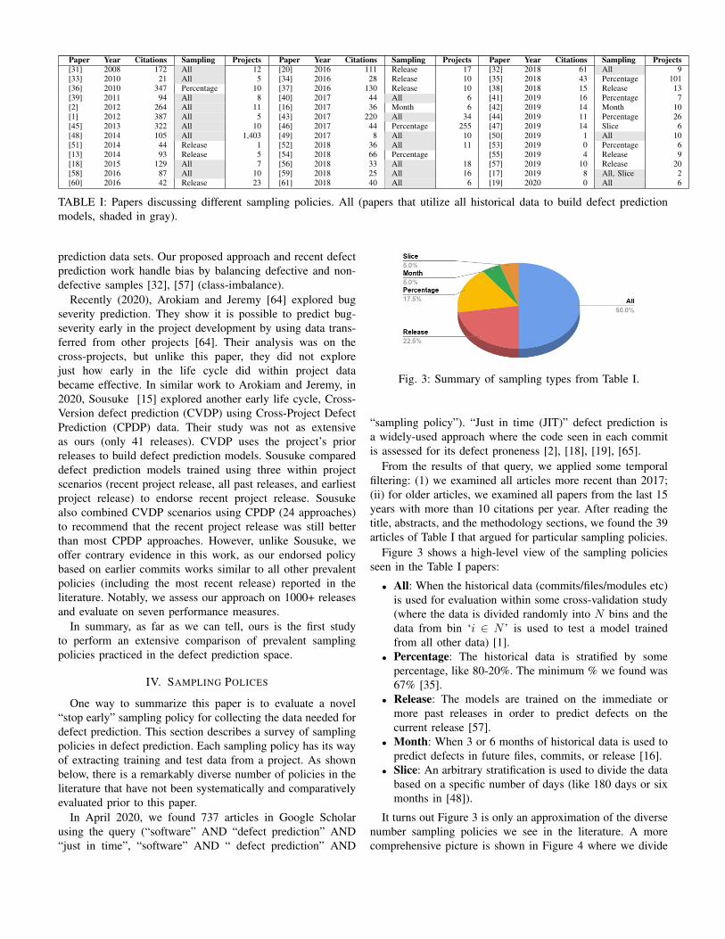
Paper Year Citations Sampling Projects Paper Year Citations Sampling Projects Paper Year Citations Sampling Projects[31] 2008 172 All 12 [20] 2016 111 Release 17 [32] 2018 61 All 9[33] 2010 21 All 5 [34] 2016 28 Release 10 [35] 2018 43 Percentage 101[36] 2010 347 Percentage 10 [37] 2016 130 Release 10 [38] 2018 15 Release 13[39] 2011 94 All 8 [40] 2017 44 All 6 [41] 2019 16 Percentage 7[2] 2012 264 All 11 [16] 2017 36 Month 6 [42] 2019 14 Month 10[1] 2012 387 All 5 [43] 2017 220 All 34 [44] 2019 11 Percentage 26[45] 2013 322 All 10 [46] 2017 44 Percentage 255 [47] 2019 14 Slice 6[48] 2014 105 All 1,403 [49] 2017 8 All 10 [50] 2019 1 All 10[51] 2014 44 Release 1 [52] 2018 36 All 11 [53] 2019 0 Percentage 6[13] 2014 93 Release 5 [54] 2018 66 Percentage [55] 2019 4 Release 9[18] 2015 129 All 7 [56] 2018 33 All 18 [57] 2019 10 Release 20[58] 2016 87 All 10 [59] 2018 25 All 16 [17] 2019 8 All, Slice 2[60] 2016 42 Release 23 [61] 2018 40 All 6 [19] 2020 0 All 6

TABLE I: Papers discussing different sampling policies. All (papers that utilize all historical data to build defect predictionmodels, shaded in gray).

prediction data sets. Our proposed approach and recent defectprediction work handle bias by balancing defective and non-defective samples [32], [57] (class-imbalance).

Recently (2020), Arokiam and Jeremy [64] explored bugseverity prediction. They show it is possible to predict bug-severity early in the project development by using data trans-ferred from other projects [64]. Their analysis was on thecross-projects, but unlike this paper, they did not explorejust how early in the life cycle did within project databecame effective. In similar work to Arokiam and Jeremy, in2020, Sousuke [15] explored another early life cycle, Cross-Version defect prediction (CVDP) using Cross-Project DefectPrediction (CPDP) data. Their study was not as extensiveas ours (only 41 releases). CVDP uses the project’s priorreleases to build defect prediction models. Sousuke compareddefect prediction models trained using three within projectscenarios (recent project release, all past releases, and earliestproject release) to endorse recent project release. Sousukealso combined CVDP scenarios using CPDP (24 approaches)to recommend that the recent project release was still betterthan most CPDP approaches. However, unlike Sousuke, weoffer contrary evidence in this work, as our endorsed policybased on earlier commits works similar to all other prevalentpolicies (including the most recent release) reported in theliterature. Notably, we assess our approach on 1000+ releasesand evaluate on seven performance measures.

In summary, as far as we can tell, ours is the first studyto perform an extensive comparison of prevalent samplingpolicies practiced in the defect prediction space.

IV. SAMPLING POLICES

One way to summarize this paper is to evaluate a novel“stop early” sampling policy for collecting the data needed fordefect prediction. This section describes a survey of samplingpolicies in defect prediction. Each sampling policy has its wayof extracting training and test data from a project. As shownbelow, there is a remarkably diverse number of policies in theliterature that have not been systematically and comparativelyevaluated prior to this paper.

In April 2020, we found 737 articles in Google Scholarusing the query (“software” AND “defect prediction” AND“just in time”, “software” AND “ defect prediction” AND

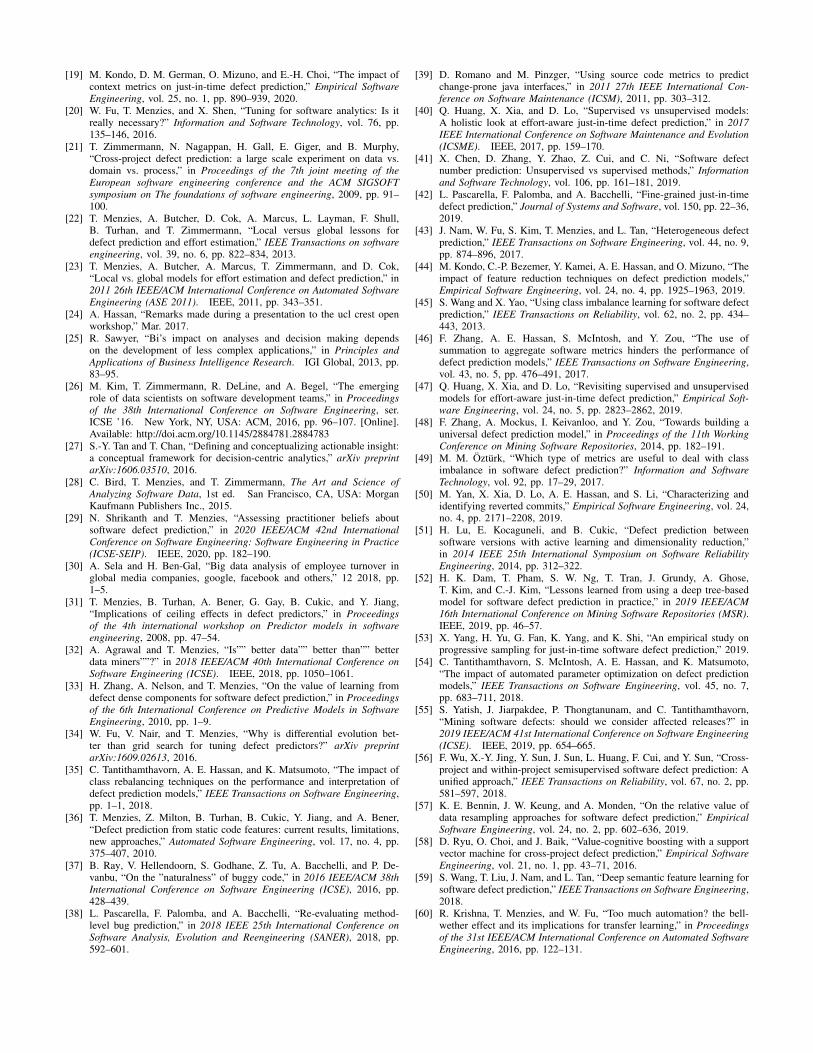
Fig. 3: Summary of sampling types from Table I.

“sampling policy”). “Just in time (JIT)” defect prediction isa widely-used approach where the code seen in each commitis assessed for its defect proneness [2], [18], [19], [65].

From the results of that query, we applied some temporalfiltering: (1) we examined all articles more recent than 2017;(ii) for older articles, we examined all papers from the last 15years with more than 10 citations per year. After reading thetitle, abstracts, and the methodology sections, we found the 39articles of Table I that argued for particular sampling policies.

Figure 3 shows a high-level view of the sampling policiesseen in the Table I papers:

• All: When the historical data (commits/files/modules etc)is used for evaluation within some cross-validation study(where the data is divided randomly into N bins and thedata from bin ‘i ∈ N ’ is used to test a model trainedfrom all other data) [1].

• Percentage: The historical data is stratified by somepercentage, like 80-20%. The minimum % we found was67% [35].

• Release: The models are trained on the immediate ormore past releases in order to predict defects on thecurrent release [57].

• Month: When 3 or 6 months of historical data is used topredict defects in future files, commits, or release [16].

• Slice: An arbitrary stratification is used to divide the databased on a specific number of days (like 180 days or sixmonths in [48]).

It turns out Figure 3 is only an approximation of the diversenumber sampling policies we see in the literature. A morecomprehensive picture is shown in Figure 4 where we divide

Fig. 4: A visual map of sampling. Project time-line dividedinto ‘Train commits’ and ‘Test commits’. Learners learn from‘Train’ to classify defective commits in the ‘Test’.

software releases Ri that occur over many months Mj intosome train and test set.

Using a little engineering judgment and guided by thefrequency of different policies (from Figure 3), we electedto focus on four sampling policies from the literature and one‘early stopping’ policy, see Table II). The % share in Figure 3show ‘ALL and RR’ are prevalent practices whereas ‘M3 andM6’ though not prevalent are used in related literature [16],[17]. We did not consider separate policies for ‘Percentage’and ‘Slice’ as the former is similar to ‘ALL’ (100% ofhistorical data), and the latter is least prevalent and similarto M6 (180 days or six months).

Note the “magic numbers” in Table II:• 3 months, 6 months: these are thresholds often seen in

the literature.• 25 clean + 25 defective commits: We arrived at these

numbers based on the work of Nam et al. built defectprediction models for using just 50 samples [43].

• Sampling at random from the first 150 commits. Here,we did some experiments recursively dividing the data inhalf until defect prediction stopped working.

We will show below that early sampling (shown in gray inTable II) works just as well as the other policies.

V. METHODS

A. Data

This section describes the data used in this study as well aswhat we mean by “clean” and “defective” commits.

All our data comes from open source (OS) GitHubprojects [7] that we mined randomly using Commit Guru [66].

Fig. 5: Distributions seen in all 1.2 millions commits of all155 projects: median values of commits (3,728), percent ofdefective commits (20%), life span in years (7), releases (59)and stars (9,149).

Commit Guru is a publicly available tool based on a 2015ESEC/FSE paper used in numerous prior works [19], [67].Commit Guru provides a portal where it takes a request (URL)to process a GitHub repository. It extracts all commits andtheir features to be exported to a file. Commits are categorized(based on the occurrence of certain keywords) similar tothe approach in SZZ algorithm [68]. The “defective” (bug-inducing) commits are traced using the git diff (show changesbetween commits) feature from bug fixing commits; the restare labeled “clean”.

But data from Commit Guru does not contain releaseinformation, which we extract separately from the project tags.Then we use scripts to associate the commits to the releasedates. Then those codes associated with those changes werethen summarized by Commit Guru using the attributes ofTable III. Those attributes became the independent attributesused in our analysis. Note that the use of these particularattributes has been endorsed by prior studies [2], [69].

SE researchers have warned against using all GitHub datasince this website contains many projects that might becategories as “non-serious” (such as homework assignments).Accordingly, following the advice of prior researchers [4], [5],we ignored projects with

• Less than 1000 stars;• Less than 1% defects;• Less than two releases;• Less than one year of activity;• No license information.• Less than 5 defective and 5 clean commits.

This resulted in 155 projects developed written in manylanguages across various domains, as discussed in §I.

Figure 5 shows information on our selected projects. Asshown in that figure, our projects have:

• Median life spans of 84 months with 59 releases;• The projects have (265, 3,728, 83,409) commits (min,

median, max) with data up to December 2019;

TABLE II: Four representative sampling policies from literature and an early life cycle policies (the row shown in gray).

Policy MethodALL Train using all past software commits ([0, Ri)) in the project before the first commit in the release under test Ri.M6 Train using the recent six months of software commits ([Ri − 6months)) made before the first commit in the release under test Ri.M3 Train using the recent three months of software commits ([Ri − 3months)) made before the first commit in the release under test Ri.RR Train using the software commits in the previous release Ri−1 before the first commit in the release under test Ri.E Train using early 50 commits (25 clean and 25 defective) randomly sampled within the first 150 commits before the first commit in the

release under test Ri.

TABLE III: 14 Commit level features that Commit Guru tool[2], [66] mines from GitHub repositories

Dimension Feature DefinitionNS Number of modified subsystemsND Number of modified directoriesNF Number of modified FilesDiffusion

ENTROPY Distribution of modified code across each fileLA Lines of code addedLD Lines of code deletedSizeLT Lines of code in a file before the change

Purpose FIX Whether the change is defect Changes that fixingthe defect are more likely to introduce more de-fects fixing ?

NDEV Number of developers that changed the modifiedfiles

AGE The average time interval from the last to thecurrent changeHistory

NUC Number of unique changes to the modified filesbefore

EXP Developer experienceREXP Recent developer experienceExperienceSEXP Developer experience on a subsystem

Fig. 6: Distributions seen in the first 150 commits of all155 projects; median values of project releases (5), projectdevelopment months (4) and defective commits (41)

• 20% (median) of project commits introduce bugs.Figure 6 focuses on just the data used in the early life cycle” E ” sampler described in Figure 4. In the median case, bythe time we can collect 150 commits, projects have had fivereleases in 4 months (median values).

B. Algorithms

Our study uses three sets of algorithms:• The five sampling policies described above;• The six classifiers described here;• Pre-processing for some of the sampling policies.1) Classifiers: After an extensive analysis, Ghotra et al.

[70] rank over 30 defect prediction algorithms into four ranks.For our work, we take six of their learners that are widely usedin the literature and which can be found at all four ranks ofthe Ghtora et al., study. Those learners were:

• Logistic Regression (LR);• Nearest neighbour (KNN) (minimum 5 neighbors);• Decision Tree (DT);• Random Forrest (RF)• Naıve Bayes (NB);• Support Vector Machines (SVM)2) Pre-processers: Following some advice from the litera-

ture, we applied some feature engineering to the Table III data.Based on advice by Nagappan and Ball, we generated relativechurn and normalized LA and LD attributes by dividing byLT and LT and NUC dividing by NF [71]. Also, we droppedND and REXP since Kamei et al. reported that NF and NDare highly correlated with REXP and EXP. Lastly, we appliedthe logarithmic transform to the remaining process measures(except the boolean variable ‘FIX’) to alleviate skewness [72].

In other pre-processing steps, we applied Correlation-basedFeature Selection (CFS). Our initial experiments with thisdata set lead to unpromising results (recalls less than 40%,high false alarms). However, those results improved after weapplied feature subset selection to remove spurious attributes.CFS is a widely applied feature subset selection method pro-posed by Hall [73] and is recommended in building superviseddefect prediction models [44]. CFS is a heuristic-based methodto find (evaluate) a subset of features incrementally. CFSperforms a best-first search to find influential sets of featuresthat are not correlated with each other, however, correlatedwith the classification. Each subset is computed as follows:merits = krcf /

√k + k(k − 1)rff where:

• merits is the value of subset s with k features;• rcf is a score that explains the connection of that feature

set to the class;• rff is the feature to feature mean and connection between

the items in s, where rcf should be large and rff .Another pre-processor that was applied to some samplingpolicies was Synthetic Minority Over-Sampling, or SMOTE.When the proportion of defective and clean commits (ormodules, files, etc.) is not equal, learners can struggle to findthe target class. SMOTE, proposed by Chawla et al. [74] isoften applied in defect prediction literature to overcome thisproblem [32], [54]. To achieve balance, SMOTE artificiallysynthesizes examples (commits) extrapolating using K-nearestneighbors (minimum five commits required) in the data set(training commits in our case) [74]. Note that:

• We do not apply SMOTE to policies that already guaran-tee class balancing. For example, our preferred early life-cycle method selects at random 25 defective, and 25 non-defective (clean) commits from the first 150 commits.

• Also, just to document that we avoided a potentialmethodological error [32], we record here that we appliedSMOTE to the training data, but never the test data.

C. Evaluation Criteria

Defect prediction studies evaluated their model performanceusing a variety of criteria. From the literature, we used whatwe judged to be the most widely-used measures [1], [2], [16],[19], [31], [35], [45], [46], [48], [50], [54], [55], [57]. For thefollowing seven criteria:

• Nearly all have the range 0 to 1 (except Initial numberof False Alarms, which can be any positive number);

• Four of these criteria need to be minimized: D2H, IFA,Brier, PF; i.e., for these criteria less is better.

• Three of these criteria need to be maximized: AUC,Recall, G-Measure; i.e. for these criteria more is better.

One reason we avoid precision is that prior work shows thismeasure has significant issues for unbalanced data [31].

1) Brier: Recent defect prediction papers [16], [19], [35],[54] measure the model performance using the Brier absolutepredictive accuracy measure. Let C be the total numberof the test commits. Let yi be 1 (for defective commits)or 0 otherwise. Let yi be the probability of commit beingdefective (calculated from the loss functions in scikit-learnclassifiers [75]). Then:

Brier =1

C

C∑t=1

(yi − yi)2 (1)

2) Initial number of False Alarms (IFA): Parnin and Orso[76] say that developers lose faith in analytics if they see toomany initial false alarms. IFA is simply the number of falsealarms encountered after sorting the commits in the order ofprobability of being detective, then counting the number offalse alarms before finding the first true alarm.

3) Recall: Recall is the proportion of inspected defectivecommits among all the actual defective commits.

Recall =True Positives

True Positives + False Negatives(2)

4) False Positive Rate (PF): The proportion of predicteddefective commits those are not defective among all thepredicted defective commits.

PF =False Positives

False Positives + True Negatives(3)

5) Area Under the Receiver Operating Characteristic curve(AUC): AUC is the area under the curve between the truepositive rate and false-positive rate.

6) Distance to Heaven (D2H): D2H or “distance to heaven”aggregates on two metrics Recall and False Positive Rate (PF)to show how close to “heaven” (Recall=1 and PF=0) [77].

D2H =

√(1− Recall)2 + (0− PF )2

√2

(4)

7) G-measure (GM): A harmonic mean between Recall andthe compliment of PF measured, as shown below.

G −Measure =2 ∗ Recall ∗ (1− PF )

Recall + (1− PF )(5)

Even though GM and D2H combined the same underlyingmeasures, we include both here since they both have beenused separately in the literature. Also, as shown below, it isnot necessarily true that achieving good results on GM meansthat good results will also be achieved with D2H.

Due to the nature of the classification process, some criteriawill always offer contradictory results:

• A learner can achieve 100% recall just by declaring thatall examples belong to the target class. This method willincur a high false alarm rate.

• A learner can achieve 0% false alarms just by declaringthat no examples belong to the target class. This methodwill incur a very low recall rate.

• Similarly, Brier and Recall are also antithetical sincereducing the loss function also means missing someconclusions and lowering recall.

D. Statistical Test

Later in §VI, we compare distributions of evaluation mea-sures of various sampling policies that may have the samemedian while their distribution could be very different. Henceto identify significant differences (rank) among two or morepopulations, we use the Scott-Knott test recommended byMittas et al. in TSE’13 paper [78]. This test is a top-down bi-clustering approach for ranking different treatments, samplingpolicies in our case. This method sorts a list of l samplingpolicy evaluations with ls measurements by their medianscore. It then splits l into sub-lists m, n in order to maximizethe expected value of differences in the observed performancesbefore and after divisions.

For lists l,m, n of size ls,ms,ns where l = m ∪ n, the“best” division maximizes E(∆); i.e. the difference in theexpected mean value before and after the spit:

E(∆) =ms

lsabs(m.µ− l.µ)2 +

ns

lsabs(n.µ− l.µ)2

We also employ the conjunction of bootstrapping and A12effect size test by Vargha and Delaney [79] to avoid “smalleffects” with statistically significant results.

Important note: we apply our statistical methods separatelyto all the evaluation criteria; i.e., when we compute ranks, wedo so for (say) false alarms separately to recall.

E. Experimental Rig

By definition, our different sampling policies have differenttrain and different test sets. But, methodologically, when wecompare these different policies, we have to compare resultson the same sets of releases. To handle this we:

• First, run all our six policies, combined with all oursix learners. This offers multiple predictions to differentcommits.

• Next, for each release, we divide the predictions intothose that come from the same learner:policy pair. Thesedivisions are then assessed with statistical methods de-scribed above.

VI. RESULTS

Tables IV and V show results when our six learners appliedour five sampling policies. We splot these results into twotables since Our policies lead to results with different samplessizes: the recent release, or “RR”, the policy uses data fromjust two releases while “ALL” uses everything.

In the first row of those tables, “+” and “-” denote criteriathat need to be maximized or minimized, respectively. Withinthe tables, gray cells show statistical test results (conductedseparately on each criterion). Anything ranked “best” is col-ored gray, while all else have white backgrounds.

Columns one and two show the policy/learners that lead tothese results. Rows are sorted by how often policy/learners“win”; i.e., achieve best ranks across all criteria. In Tables IVand V, no policy+learner wins 7 out of 7 times on allcriteria, so some judgment will be required to make anoverall conclusion. Specifically, based on results from themulti-objective optimization literature, we will first removethe policies+learners that score worse on most criteria, thendebate trade-offs between the rest.

To simplify that trade-off debate, we offer two notes. Firstly,cross all our learners, the median value for IFA is very small–zero or one; i.e., developers using these tools only need tosuffer one false alarm or less before finding something theyneed to fix. Since these observed IFA scores are so small,we say that “losing” on IFA is hardly a reason to dismiss alearner/sampler combination. Secondly, D2H and GM combinemultiple criteria. For example, “winning” on D2H and GMmeans performing well on both Recall and PF; i.e. these twocriteria are somewhat more informative than the others.

Turning now to those results, we explore two issues. Fordefect prediction:RQ1: Is more data, better?RQ2: When is more recent data better than older data?

Note that we do explore a third research issue: are differentlearners better at learning from a little, a lot, or all theavailable data. Based on our results, we have nothing definitiveto offer on that issue. That said, if we were pressed torecommend a particular learning algorithm, then we say thereare no counterexamples to the claim that “it is useful to applyCFS+LR”.

RQ1: Is more data, better?

Belief1: Our introduction included examples where propo-nents of data-hungry methods advocated that if data is useful,then even more data is much more useful.

Prediction:1 If that belief was the case, then in Table IV,data-hungry sampling policies that used more data shoulddefeat “data-lite” sampling policies.

Observation1a: In Table IV, Our “data hungriest” samplingpolicy (ALL) loses on on most criteria. While it achieves the

highest Recall (83%), it also has the highest false alarm range(40%). As to which other policy is preferred in the best wins=4zone of Table IV, there is no clear winner. What we wouldsay here is that our preferred “data-lite” method called “E”(that uses 25 defective and 25 non-defective commits selectedat random from the first 150 commits) is competitive with therest. Hence:

Answer1a: For defect prediction, it is not clear thatmore data is inherently better.

Observations1b: Figure 5 of this paper showed that withinour sample of projects, we have data lasting a median of84 months. Figure 6 noted that by the time we get to 150commits, most projects are 4 months old (median values). The“E” results of Table IV showed that defect models learnedfrom that 4 months of data are competitive with all the otherpolicies studied here. Hence we say,

Answer1b: 96% of the time, we do not want and wedo not need data-hungry methods

RQ2: When is more recent data better than older data?

Belief2: As discussed earlier in our introduction, manyresearchers prefer using recent data over data from earlierperiods. For example, it is common practice in defect predic-tion to perform “recent validation” where predictors are testedon the latest release after training from the prior one or tworeleases [16], [18]–[20]. For a project with multiple releases,recent validation ignores all the insights that are available fromolder releases.

Prediction2: If recent data is comparatively more informa-tive than older data, then defect predictors built on recent datashould out-perform predictors built on much older data.

Observations2: We observe that:• Figure 5 of this paper showed that within our sample of

projects, we have data lasting a median of 84 months.• Figure 6 noted that by the time we get to 150 commits,

most projects are 4 months old (median values).• Table V says that “E” wins over “RR” since it falls in

the best wins=4 section.• Hence we could conclude that older data is more effective

than recent data.That said, we feel somewhat more the circumspect conclusionis in order. When we compare E+LR to the next learner inthat table (RR+NB) we only find a minimal difference intheir performance scores. Hence we make a somewhat humblerconclusion:

Answer2: Recency based methods perform no betterthan results from early life cycle defect predictors.

This is a startling result for two reasons. Firstly, comparedto the “RR” training data, the “E” training data is very oldindeed. For projects lasting 84 months long, “RR” is trained

on information from recent few months, with “E” data comesfrom years before that. Secondly, this result calls into questionany conclusion made in a paper that used recent validation toassess their approach; e.g. [16], [18]–[20].

VII. THREATS TO VALIDITY

A. Sampling Bias

The conclusion’s generalizability will depend upon thesamples considered; i.e., what matters here may not be trueeverywhere. To improve our conclusion’s generalizability, wemined 155 long-running OS projects that are developed for

disparate domains and written in numerous programming lan-guages. Sampling trivial projects (like homework assignments)is a potential threat to our analysis. To mitigate that, weadhered to the advice from prior researchers as discussedearlier in §I and §V-A. We find our sample of projects have20% (median) defects as shown in Figure 5 nearly the sameas data used by Tantithamthavorn et al. [35] who report 30%(median) defects.

B. Learner bias

Any single study can only explore a handful of classificationalgorithms. For building the defect predictors in this work, we

Policy Classifier Wins D2H- AUC+ IFA- Brier- Recall+ PF- GM+M6 NB

4

0.37 0.67 1.0 0.32 0.78 0.33 0.67M3 NB 0.37 0.67 1.0 0.31 0.76 0.32 0.68E LR 0.36 0.68 1.0 0.32 0.71 0.31 0.68M6 SVM 0.43 0.65 0.0 0.21 0.44 0.1 0.48M3 SVM 0.43 0.65 0.0 0.21 0.43 0.1 0.48ALL NB 3 0.4 0.65 1.0 0.36 0.83 0.40 0.67E KNN

2

0.39 0.65 1.0 0.33 0.65 0.32 0.62ALL LR 0.38 0.66 1.0 0.3 0.65 0.25 0.62M6 LR 0.36 0.68 1.0 0.25 0.59 0.19 0.60M3 LR 0.36 0.68 1.0 0.24 0.58 0.17 0.60M6 KNN 0.4 0.65 0.0 0.23 0.50 0.14 0.53ALL SVM 0.4 0.66 0.0 0.25 0.50 0.14 0.54M3 KNN 0.41 0.65 0.0 0.23 0.47 0.13 0.51M6 RF 0.44 0.63 0.0 0.24 0.43 0.12 0.47E SVM

1

0.4 0.64 1.0 0.31 0.6 0.26 0.59ALL KNN 0.38 0.66 1.0 0.25 0.55 0.17 0.57ALL DT 0.42 0.62 1.0 0.32 0.52 0.25 0.54M6 DT 0.43 0.62 1.0 0.29 0.5 0.2 0.51ALL RF 0.42 0.64 1.0 0.26 0.49 0.15 0.51M3 DT 0.43 0.62 1.0 0.28 0.48 0.19 0.5M3 RF 0.44 0.63 1.0 0.24 0.42 0.11 0.46E DT

00.46 0.58 1.0 0.38 0.57 0.35 0.54

E NB 0.54 0.54 1.0 0.37 0.55 0.29 0.41E RF 0.44 0.61 1.0 0.33 0.52 0.26 0.52

KEY: More data (ALL,M6 and M3) Early (E)

TABLE IV: 24 defect prediction models tested in all 4,876 applicable project releases. In the first row “+” and “-” denotethe criteria that need to be maximized or minimized, respectively. ‘Wins’ is the frequency of the policy found in the top #1Scott-Knott rank in each of the seven evaluation measures (the cells shaded in gray).

Policy Classifier Wins D2H- AUC+ IFA- Brier- Recall+ PF- GM+E LR 4 0.36 0.68 1.0 0.32 0.71 0.31 0.68RR NB 3 0.38 0.66 1.0 0.32 0.71 0.30 0.65RR LR 3 0.35 0.68 1.0 0.24 0.59 0.18 0.61RR SVM 3 0.42 0.64 0.0 0.23 0.47 0.12 0.5E KNN 2 0.39 0.64 1.0 0.34 0.64 0.32 0.62RR KNN 2 0.41 0.64 1.0 0.25 0.5 0.15 0.53RR RF 2 0.43 0.63 1.0 0.24 0.43 0.13 0.48E SVM 1 0.4 0.64 1.0 0.31 0.6 0.26 0.59E DT 0 0.46 0.58 1.0 0.39 0.56 0.35 0.54E NB 0 0.54 0.54 1.0 0.37 0.54 0.29 0.42E RF 0 0.44 0.61 1.0 0.33 0.52 0.26 0.53RR DT 0 0.42 0.62 1.0 0.28 0.50 0.20 0.51

KEY: Recency (RR) Early (E)

TABLE V: 12 defect prediction models tested on 3,704 project releases. In the first row “+” and “-” denote criteria that needto be maximized or minimized, respectively. ‘Wins’ is the frequency of the policy found in the top #1 Scott-Knott rank ineach of the seven evaluation measures (the cells shaded in gray).

elected six learners (Logistic Regression, Nearest neighbor,Decision Tree, Support Vector Machines, Random Forrest,and Naıve Bayes). These six learners represent a plethora ofclassification algorithms [70].

C. Evaluation bias

We use seven evaluation measures (Recall, PF, IFA, Brier,GM, D2H, and AUC). Other prevalent measures in this defectprediction space include precision. However, as mentionedearlier, precision has issues with unbalanced data [31].

D. Input Bias

Our proposed sampling policy ‘E’ randomly samples 50commits from early 150 commits. Thus it may be true thatdifferent executions could yield different results. However,this is not a threat because each time, the early policy ‘E ’randomly samples 50 commits from early 150 commits to testsizeable 8,490 releases (from Table IV and Table V) acrossall the six learners. In other words, our conclusions about ‘E’hold on a large sample size of numerous releases.

VIII. CONCLUSION

When data keep changing, the models we can learn fromthat data may also change. If conclusions become too fluid(i.e., change too often), then no one has a stable basis formaking decisions or communicating insights.

Issues with conclusion instability disappear if, early in thelife cycle, we can learn a predictive model that is effective forthe rest of the project. This paper has proposed a methodologyfor assessing such early life cycle predictors.

1) Define a project selection criteria. For this paper, ourselection criteria are taken from related work (fromrecent EMSE, TSE papers [4], [5]);

2) Select some software analytics task. For this paper, wehave explored learning defect predictors.

3) See how early projects selected by the criteria canbe modeled for that task. Here we found that defectpredictors learned from the first four months of dataperform as well as anything else.

4) Conclude that projects matching criteria need more datafor task before time found in step 3. In this paper, wefound that for 96% of the time, we neither want norneed data-hungry defect prediction.

We stress that this result has only been shown here for defectprediction and only for the data selected by our criteria.

As for future work, we have many suggestions:• The clear next step in this work is to check the validity

of this conclusion beyond the specific criteria and taskexplored here.

• We need to revisit all prior results that used recentvalidation to assess their approach; e.g. [16], [18]–[20]since our RQ2 suggests they may have been working ina relatively uninformative region of the data.

• While the performance scores of Tables IV and V arereasonable, there is still much room for improvement.Perhaps if we augmented early life cycle defect predictors

with a little transfer learning (from other projects [43]),then we could generate better performing predictors.

• Further to the last point, another interesting avenue offuture research might be hyper-parameter optimization(HPO) [20], [80], [81]. HPO is often not applied insoftware analytics due to its computational complexity.Perhaps that complexity can be avoided by focusing onlyon small samples of data from very early in the life cycle.

ACKNOWLEDGEMENTS

This work was partially supported by NSF grant #1908762.

REFERENCES

[1] M. D’Ambros, M. Lanza, and R. Robbes, “Evaluating defect predictionapproaches: a benchmark and an extensive comparison,” EmpiricalSoftware Engineering, vol. 17, no. 4-5, pp. 531–577, 2012.

[2] Y. Kamei, E. Shihab, B. Adams, A. E. Hassan, A. Mockus, A. Sinha,and N. Ubayashi, “A large-scale empirical study of just-in-time qualityassurance,” IEEE Transactions on Software Engineering, vol. 39, no. 6,pp. 757–773, 2012.

[3] P. Norvig. (2011) The Unreasonable Effectiveness of Data. Youtube.[Online]. Available: https://www.youtube.com/watch?v=yvDCzhbjYWs

[4] N. Munaiah, S. Kroh, C. Cabrey, and M. Nagappan, “Curating github forengineered software projects,” Empirical Software Engineering, vol. 22,no. 6, pp. 3219–3253, 2017.

[5] M. Yan, X. Xia, Y. Fan, A. E. Hassan, D. Lo, and S. Li, “Just-in-timedefect identification and localization: A two-phase framework,” IEEETransactions on Software Engineering, 2020.

[6] R. Abdalkareem, V. Oda, S. Mujahid, and E. Shihab, “On the impactof using trivial packages: an empirical case study on npm and pypi,”Empirical Software Engineering, vol. 25, no. 2, pp. 1168–1204, Mar.2020. [Online]. Available: https://doi.org/10.1007/s10664-019-09792-9

[7] “GitHub Inc - provides hosting for software development version controlusing git.” https://github.com/, accessed: 2019-03-18.

[8] T. J. Ostrand, E. J. Weyuker, and R. M. Bell, “Predicting the locationand number of faults in large software systems,” IEEE Transactions onSoftware Engineering, vol. 31, no. 4, pp. 340–355, 2005.

[9] T. Menzies, J. Greenwald, and A. Frank, “Data mining static codeattributes to learn defect predictors,” IEEE transactions on softwareengineering, vol. 33, no. 1, pp. 2–13, 2006.

[10] Z. Wan, X. Xia, A. E. Hassan, D. Lo, J. Yin, and X. Yang, “Perceptions,expectations, and challenges in defect prediction,” IEEE Transactions onSoftware Engineering, 2018.

[11] A. T. Misirli, A. Bener, and R. Kale, “Ai-based software defect predic-tors: Applications and benefits in a case study,” AI Magazine, vol. 32,no. 2, pp. 57–68, 2011.

[12] M. Kim, D. Cai, and S. Kim, “An empirical investigation into the role ofapi-level refactorings during software evolution,” in Proceedings of the33rd International Conference on Software Engineering. ACM, 2011,pp. 151–160.

[13] F. Rahman, S. Khatri, E. T. Barr, and P. Devanbu, “Comparing staticbug finders and statistical prediction,” in Proceedings of the 36thInternational Conference on Software Engineering, ser. ICSE 2014.New York, NY, USA: Association for Computing Machinery, 2014, p.424–434. [Online]. Available: https://doi.org/10.1145/2568225.2568269

[14] F. Rahman, D. Posnett, I. Herraiz, and P. Devanbu, “Sample size vs.bias in defect prediction,” in Proceedings of the 2013 9th joint meetingon foundations of software engineering. ACM, 2013, pp. 147–157.

[15] S. Amasaki, “Cross-version defect prediction: use historical data, cross-project data, or both?” Empirical Software Engineering, pp. 1–23, 2020.

[16] S. McIntosh and Y. Kamei, “Are fix-inducing changes a moving target?a longitudinal case study of just-in-time defect prediction,” IEEE Trans-actions on Software Engineering, vol. 44, no. 5, pp. 412–428, 2017.

[17] T. Hoang, H. Khanh Dam, Y. Kamei, D. Lo, and N. Ubayashi, “Deepjit:An end-to-end deep learning framework for just-in-time defect predic-tion,” in 2019 IEEE/ACM 16th International Conference on MiningSoftware Repositories (MSR), 2019, pp. 34–45.

[18] M. Tan, L. Tan, S. Dara, and C. Mayeux, “Online defect predictionfor imbalanced data,” in 2015 IEEE/ACM 37th IEEE InternationalConference on Software Engineering, vol. 2. IEEE, 2015, pp. 99–108.

[19] M. Kondo, D. M. German, O. Mizuno, and E.-H. Choi, “The impact ofcontext metrics on just-in-time defect prediction,” Empirical SoftwareEngineering, vol. 25, no. 1, pp. 890–939, 2020.

[20] W. Fu, T. Menzies, and X. Shen, “Tuning for software analytics: Is itreally necessary?” Information and Software Technology, vol. 76, pp.135–146, 2016.

[21] T. Zimmermann, N. Nagappan, H. Gall, E. Giger, and B. Murphy,“Cross-project defect prediction: a large scale experiment on data vs.domain vs. process,” in Proceedings of the 7th joint meeting of theEuropean software engineering conference and the ACM SIGSOFTsymposium on The foundations of software engineering, 2009, pp. 91–100.

[22] T. Menzies, A. Butcher, D. Cok, A. Marcus, L. Layman, F. Shull,B. Turhan, and T. Zimmermann, “Local versus global lessons fordefect prediction and effort estimation,” IEEE Transactions on softwareengineering, vol. 39, no. 6, pp. 822–834, 2013.

[23] T. Menzies, A. Butcher, A. Marcus, T. Zimmermann, and D. Cok,“Local vs. global models for effort estimation and defect prediction,” in2011 26th IEEE/ACM International Conference on Automated SoftwareEngineering (ASE 2011). IEEE, 2011, pp. 343–351.

[24] A. Hassan, “Remarks made during a presentation to the ucl crest openworkshop,” Mar. 2017.

[25] R. Sawyer, “Bi’s impact on analyses and decision making dependson the development of less complex applications,” in Principles andApplications of Business Intelligence Research. IGI Global, 2013, pp.83–95.

[26] M. Kim, T. Zimmermann, R. DeLine, and A. Begel, “The emergingrole of data scientists on software development teams,” in Proceedingsof the 38th International Conference on Software Engineering, ser.ICSE ’16. New York, NY, USA: ACM, 2016, pp. 96–107. [Online].Available: http://doi.acm.org/10.1145/2884781.2884783

[27] S.-Y. Tan and T. Chan, “Defining and conceptualizing actionable insight:a conceptual framework for decision-centric analytics,” arXiv preprintarXiv:1606.03510, 2016.

[28] C. Bird, T. Menzies, and T. Zimmermann, The Art and Science ofAnalyzing Software Data, 1st ed. San Francisco, CA, USA: MorganKaufmann Publishers Inc., 2015.

[29] N. Shrikanth and T. Menzies, “Assessing practitioner beliefs aboutsoftware defect prediction,” in 2020 IEEE/ACM 42nd InternationalConference on Software Engineering: Software Engineering in Practice(ICSE-SEIP). IEEE, 2020, pp. 182–190.

[30] A. Sela and H. Ben-Gal, “Big data analysis of employee turnover inglobal media companies, google, facebook and others,” 12 2018, pp.1–5.

[31] T. Menzies, B. Turhan, A. Bener, G. Gay, B. Cukic, and Y. Jiang,“Implications of ceiling effects in defect predictors,” in Proceedingsof the 4th international workshop on Predictor models in softwareengineering, 2008, pp. 47–54.

[32] A. Agrawal and T. Menzies, “Is”” better data”” better than”” betterdata miners””?” in 2018 IEEE/ACM 40th International Conference onSoftware Engineering (ICSE). IEEE, 2018, pp. 1050–1061.

[33] H. Zhang, A. Nelson, and T. Menzies, “On the value of learning fromdefect dense components for software defect prediction,” in Proceedingsof the 6th International Conference on Predictive Models in SoftwareEngineering, 2010, pp. 1–9.

[34] W. Fu, V. Nair, and T. Menzies, “Why is differential evolution bet-ter than grid search for tuning defect predictors?” arXiv preprintarXiv:1609.02613, 2016.

[35] C. Tantithamthavorn, A. E. Hassan, and K. Matsumoto, “The impact ofclass rebalancing techniques on the performance and interpretation ofdefect prediction models,” IEEE Transactions on Software Engineering,pp. 1–1, 2018.

[36] T. Menzies, Z. Milton, B. Turhan, B. Cukic, Y. Jiang, and A. Bener,“Defect prediction from static code features: current results, limitations,new approaches,” Automated Software Engineering, vol. 17, no. 4, pp.375–407, 2010.

[37] B. Ray, V. Hellendoorn, S. Godhane, Z. Tu, A. Bacchelli, and P. De-vanbu, “On the ”naturalness” of buggy code,” in 2016 IEEE/ACM 38thInternational Conference on Software Engineering (ICSE), 2016, pp.428–439.

[38] L. Pascarella, F. Palomba, and A. Bacchelli, “Re-evaluating method-level bug prediction,” in 2018 IEEE 25th International Conference onSoftware Analysis, Evolution and Reengineering (SANER), 2018, pp.592–601.

[39] D. Romano and M. Pinzger, “Using source code metrics to predictchange-prone java interfaces,” in 2011 27th IEEE International Con-ference on Software Maintenance (ICSM), 2011, pp. 303–312.

[40] Q. Huang, X. Xia, and D. Lo, “Supervised vs unsupervised models:A holistic look at effort-aware just-in-time defect prediction,” in 2017IEEE International Conference on Software Maintenance and Evolution(ICSME). IEEE, 2017, pp. 159–170.

[41] X. Chen, D. Zhang, Y. Zhao, Z. Cui, and C. Ni, “Software defectnumber prediction: Unsupervised vs supervised methods,” Informationand Software Technology, vol. 106, pp. 161–181, 2019.

[42] L. Pascarella, F. Palomba, and A. Bacchelli, “Fine-grained just-in-timedefect prediction,” Journal of Systems and Software, vol. 150, pp. 22–36,2019.

[43] J. Nam, W. Fu, S. Kim, T. Menzies, and L. Tan, “Heterogeneous defectprediction,” IEEE Transactions on Software Engineering, vol. 44, no. 9,pp. 874–896, 2017.

[44] M. Kondo, C.-P. Bezemer, Y. Kamei, A. E. Hassan, and O. Mizuno, “Theimpact of feature reduction techniques on defect prediction models,”Empirical Software Engineering, vol. 24, no. 4, pp. 1925–1963, 2019.

[45] S. Wang and X. Yao, “Using class imbalance learning for software defectprediction,” IEEE Transactions on Reliability, vol. 62, no. 2, pp. 434–443, 2013.

[46] F. Zhang, A. E. Hassan, S. McIntosh, and Y. Zou, “The use ofsummation to aggregate software metrics hinders the performance ofdefect prediction models,” IEEE Transactions on Software Engineering,vol. 43, no. 5, pp. 476–491, 2017.

[47] Q. Huang, X. Xia, and D. Lo, “Revisiting supervised and unsupervisedmodels for effort-aware just-in-time defect prediction,” Empirical Soft-ware Engineering, vol. 24, no. 5, pp. 2823–2862, 2019.

[48] F. Zhang, A. Mockus, I. Keivanloo, and Y. Zou, “Towards building auniversal defect prediction model,” in Proceedings of the 11th WorkingConference on Mining Software Repositories, 2014, pp. 182–191.

[49] M. M. Ozturk, “Which type of metrics are useful to deal with classimbalance in software defect prediction?” Information and SoftwareTechnology, vol. 92, pp. 17–29, 2017.

[50] M. Yan, X. Xia, D. Lo, A. E. Hassan, and S. Li, “Characterizing andidentifying reverted commits,” Empirical Software Engineering, vol. 24,no. 4, pp. 2171–2208, 2019.

[51] H. Lu, E. Kocaguneli, and B. Cukic, “Defect prediction betweensoftware versions with active learning and dimensionality reduction,”in 2014 IEEE 25th International Symposium on Software ReliabilityEngineering, 2014, pp. 312–322.

[52] H. K. Dam, T. Pham, S. W. Ng, T. Tran, J. Grundy, A. Ghose,T. Kim, and C.-J. Kim, “Lessons learned from using a deep tree-basedmodel for software defect prediction in practice,” in 2019 IEEE/ACM16th International Conference on Mining Software Repositories (MSR).IEEE, 2019, pp. 46–57.

[53] X. Yang, H. Yu, G. Fan, K. Yang, and K. Shi, “An empirical study onprogressive sampling for just-in-time software defect prediction,” 2019.

[54] C. Tantithamthavorn, S. McIntosh, A. E. Hassan, and K. Matsumoto,“The impact of automated parameter optimization on defect predictionmodels,” IEEE Transactions on Software Engineering, vol. 45, no. 7,pp. 683–711, 2018.

[55] S. Yatish, J. Jiarpakdee, P. Thongtanunam, and C. Tantithamthavorn,“Mining software defects: should we consider affected releases?” in2019 IEEE/ACM 41st International Conference on Software Engineering(ICSE). IEEE, 2019, pp. 654–665.

[56] F. Wu, X.-Y. Jing, Y. Sun, J. Sun, L. Huang, F. Cui, and Y. Sun, “Cross-project and within-project semisupervised software defect prediction: Aunified approach,” IEEE Transactions on Reliability, vol. 67, no. 2, pp.581–597, 2018.

[57] K. E. Bennin, J. W. Keung, and A. Monden, “On the relative value ofdata resampling approaches for software defect prediction,” EmpiricalSoftware Engineering, vol. 24, no. 2, pp. 602–636, 2019.

[58] D. Ryu, O. Choi, and J. Baik, “Value-cognitive boosting with a supportvector machine for cross-project defect prediction,” Empirical SoftwareEngineering, vol. 21, no. 1, pp. 43–71, 2016.

[59] S. Wang, T. Liu, J. Nam, and L. Tan, “Deep semantic feature learning forsoftware defect prediction,” IEEE Transactions on Software Engineering,2018.

[60] R. Krishna, T. Menzies, and W. Fu, “Too much automation? the bell-wether effect and its implications for transfer learning,” in Proceedingsof the 31st IEEE/ACM International Conference on Automated SoftwareEngineering, 2016, pp. 122–131.

[61] X. Chen, Y. Zhao, Q. Wang, and Z. Yuan, “Multi: Multi-objective effort-aware just-in-time software defect prediction,” Information and SoftwareTechnology, vol. 93, pp. 1–13, 2018.

[62] N. Fenton, M. Neil, W. Marsh, P. Hearty, Ł. Radlinski, and P. Krause,“On the effectiveness of early life cycle defect prediction with bayesiannets,” Empirical Software Engineering, vol. 13, no. 5, p. 499, 2008.

[63] H. Zhang and R. Wu, “Sampling program quality,” in 2010 IEEEInternational Conference on Software Maintenance. IEEE, 2010, pp.1–10.

[64] J. Arokiam and J. S. Bradbury, “Automatically predicting bug severityearly in the development process,” in Proceedings of the ACM/IEEE42nd International Conference on Software Engineering: New Ideas andEmerging Results, 2020, pp. 17–20.

[65] T. Fukushima, Y. Kamei, S. McIntosh, K. Yamashita, and N. Ubayashi,“An empirical study of just-in-time defect prediction using cross-projectmodels,” in Proceedings of the 11th Working Conference on MiningSoftware Repositories. ACM, 2014, pp. 172–181.

[66] C. Rosen, B. Grawi, and E. Shihab, “Commit guru: analytics and riskprediction of software commits,” in Proceedings of the 2015 10th JointMeeting on Foundations of Software Engineering. ACM, 2015, pp.966–969.

[67] X. Xia, E. Shihab, Y. Kamei, D. Lo, and X. Wang, “Predictingcrashing releases of mobile applications,” in Proceedings of the 10thACM/IEEE International Symposium on Empirical Software Engineeringand Measurement, 2016, pp. 1–10.

[68] J. Sliwerski, T. Zimmermann, and A. Zeller, “When do changes inducefixes?” in Proceedings of the 2005 International Workshop on MiningSoftware Repositories, ser. MSR ’05. New York, NY, USA: ACM,2005, pp. 1–5. [Online]. Available: http://doi.acm.org/10.1145/1082983.1083147

[69] F. Rahman and P. Devanbu, “How, and why, process metrics are better,”in 2013 35th International Conference on Software Engineering (ICSE).IEEE, 2013, pp. 432–441.

[70] B. Ghotra, S. McIntosh, and A. E. Hassan, “Revisiting the impactof classification techniques on the performance of defect predictionmodels,” in 37th ICSE-Volume 1. IEEE Press, 2015, pp. 789–800.

[71] N. Nagappan and T. Ball, “Use of relative code churn measures topredict system defect density,” in Proceedings of the 27th internationalconference on Software engineering. ACM, 2005, pp. 284–292.

[72] E. Shihab, Z. M. Jiang, W. M. Ibrahim, B. Adams, and A. E. Hassan,“Understanding the impact of code and process metrics on post-releasedefects: a case study on the eclipse project,” in Proceedings of the 2010ACM-IEEE International Symposium on Empirical Software Engineer-ing and Measurement, 2010, pp. 1–10.

[73] M. A. Hall and G. Holmes, “Benchmarking attribute selection techniquesfor discrete class data mining,” IEEE Transactions on Knowledge andData engineering, vol. 15, no. 6, pp. 1437–1447, 2003.

[74] N. V. Chawla, K. W. Bowyer, L. O. Hall, and W. P. Kegelmeyer, “Smote:synthetic minority over-sampling technique,” Journal of artificial intel-ligence research, vol. 16, pp. 321–357, 2002.

[75] F. Pedregosa, G. Varoquaux, A. Gramfort, V. Michel, B. Thirion,O. Grisel, M. Blondel, P. Prettenhofer, R. Weiss, V. Dubourg, J. Vander-plas, A. Passos, D. Cournapeau, M. Brucher, M. Perrot, and E. Duch-esnay, “Scikit-learn: Machine learning in Python,” Journal of MachineLearning Research, vol. 12, pp. 2825–2830, 2011.

[76] C. Parnin and A. Orso, “Are automated debugging techniques actuallyhelping programmers?” in Proceedings of the 2011 international sym-posium on software testing and analysis. ACM, 2011, pp. 199–209.

[77] D. Chen, W. Fu, R. Krishna, and T. Menzies, “Applications of psycho-logical science for actionable analytics,” FSE’19, 2018.

[78] N. Mittas and L. Angelis, “Ranking and clustering software costestimation models through a multiple comparisons algorithm,” IEEETrans SE, vol. 39, no. 4, pp. 537–551, Apr. 2013.

[79] A. Vargha and H. D. Delaney, “A critique and improvement of the clcommon language effect size statistics of mcgraw and wong,” Journalof Educational and Behavioral Statistics, vol. 25, no. 2, pp. 101–132,2000.

[80] C. Tantithamthavorn, S. McIntosh, A. E. Hassan, and K. Matsumoto,“Automated parameter optimization of classification techniques fordefect prediction models,” in ICSE 2016. ACM, 2016, pp. 321–332.

[81] A. Agrawal, W. Fu, D. Chen, X. Shen, and T. Menzies, “How to”dodge” complex software analytics,” IEEE Transactions on SoftwareEngineering, 2019.