* : THE AUTHORS HAVE CONTRIBUTED EQUALLY.

Early-season Vineyard Shoot and Leaf Estimation Using Computer Vision

Techniques HARJATIN SINGH BAWEJA1 *, TANVIR PARHAR2 *, STEPHEN NUSKE3

1,2,3Robotics Institute, Research Associate, Carnegie Mellon University, 5000 Forbes Avenue, Pittsburgh, 15232,

United States of America

E-MAIL: harjatis@andrew.cmu.edu, ptanvir@andrew.cmu.edu, nuske@cmu.edu

Abstract:

This paper describes computer vision techniques for

early-season measurement of vine canopy parameters; leaf

count, leaf area and shoot count. Accurate and high-

resolution estimation of these key vineyard performance

components are important for effective precision

management. We use a high-resolution stereo camera with

strobe lighting mounted on a ground-vehicle that captures

high-quality proximal images of the vines. For shoot image

segmentation, we apply the Frangi vessel filter (originally

developed for medical imaging processing) in conjunction

with custom filtering to extract shoot counts. We also

present an incremental leaf count estimation algorithm,

that proposes leaf candidates for incremental leaf sizes and

then removes the repeating candidates to accurately assess

leaf count. The specified algorithms are robust to partial

occlusion and varying lighting conditions. For shoot count

measurement we observe an F1 score of 0.85 for image

shoot count and R correlation of 0.88 for ground-truth

shoot counts. The R correlation for leaf count estimation

between ground truth sample images and algorithm output

is 0.798. Whereas the R correlation between the data

collected by a PAR sensor and leaf area estimation

algorithm is 0.69.

Keywords:

Plant Segmentation; Computer Vision; Image

processing; Precision Viticulture; Precision management;

Shoot Count; Leaf Count; Leaf Area;

1. Introduction

Vineyard cultivation industry is a large and diverse

industry. As many as 40 different varieties of grapes are known

and cultivated worldwide. The produce is used for production

of various edibles like grape juice, raisins and wine. As

reported by “International Organization of Wine and Vine”, as

of 2015 vineyards covered 7.534 million hectares of

agricultural land worldwide. To give a better perspective to the

size of the industry, according to “The Wine Institute from

TTB data”, the total wine produced by USA alone was 835.468

million gallons. Hence, such high investments and stakes

involved in the vineyard industry makes application of

technological advances in vineyard management a valuable

exercise.

Currently there are no systems available for growers to

measure crop yield with high resolution during the growing

season. Crop yield is a desirable attribute to be monitored and

managed. The current process to estimate yield is by

monitoring the farm at harvest time, and recording data during

each growing season. However, yield can vary by large

amounts from year to year, and using harvest estimates is an

extremely coarse approximation of yield. In order to get

accurate dense measures of crop yield, the crop needs to be

continuously measured during the growing season. The

obvious solution would be to exhaustively monitor the fields.

While the approach might work well for small sized fields,

it becomes economically intractable for larger fields owing to

the labor intensive nature of the work. Additionally, the manual

counting mechanism is performed just before harvest. Over the

past few years, our research group has focused on developing

a vision-based system for automatic fruit detection and high

resolution yield-estimation [1] [2]. However, this does not

include two of the major components of yield estimation and

crop management, namely shoot density and leaf area and

count measurements.

One of the most major components of precise yield

management is shoot density estimation for vines across the

field. An accurate machine vision based approach for efficient

calculation of this parameter would not only giving a vital

estimate of number of prospective fruit bearing healthy crops

this season but also be a telling parameter to monitor plant

growth and health. Leaf area and leaf count estimation, during

the early growth season helps the farmer to get a better insight

into vineyard’s overall health. Providing a farmer with geo-

localized maps of leaf count/area help the farmer in focusing

the water and nutrient resources. This in turn helps in an

increase in the yield. The reduction and optimization of

resources used in vineyard management is the motivation

behind this work

2. Related Work

Exponentially increasing population growth has resulted

in the need for proportionate increase in agricultural produce

as well. Though population is growing at an exponential rate,

the same cannot be said for cultivatable land. Thus this creates

a need for increasing output from currently available land

without overburdening it. This has led to an increased interest

in funding research in precision viticulture.

Some work has been done to obtain precise yield

estimates in vineyards by accurately measuring fruit density

measurement using classical image processing techniques

[9][10]. There have also been some successful attempts at

using purely learning based techniques such as feature-

learning based techniques [4], conditional random fields(CRFs)

[5] amongst others. However, the most successful have been

the ones using a combination of classical image processing

pipelines with learning based methods [2].

Surprisingly very little work is done on using shoot

density measurement and leaf area/count estimates to do the

same work. Some thinning based techniques have been used to

remove shoots from the rest of the plant and estimate density

[3]. There also has been an attempt at using reflection patterns

of structured light to delineate convex shapes from concave

ones thus using this technique to segment shoots from rest of

the plant. [5]. Shape fitting based stem segmentation

techniques on 3 dimensional plant models by taking advantage

of prior knowledge of plant structure have also been attempted.

[6]. The most promising approach is use of vesselness measure

of plant branches for segmentation [21]. The method provides

promising results in lab conditions, however uses the

assumption that size of plant shoot is considerably larger than

the size of leaf edges which is subject to plant type and not

robust to occlusions. Thus, this paper uses the work of Amean

et.al. [21] as baseline for shoot density measurement and

builds on that.

There have been a wide variety of attempts for estimation

of leaf count and leaf area of plants. Various methods deploy

techniques varying from image processing methods to digital

sensor based data acquisition techniques. There has been an

attempt on leaf segmentation by fitting quadratic curves to a

combination of depth data and IR data [11]. RGBD sensors like

Microsoft Kinect have been used for leaf segmentation and

leaf count estimation using center of divergence methods,

which employ parametric snakes [12][13]. But the drawback

of this approach is limitation of Kinect to indoors and the slow

convergence of parametric snakes. There exist techniques

involving a combination of log-polar transformation and

unsupervised learning using triangle encoding and K means

clustering [14, 15, 16]. But these techniques presume that

leaves are of a distinct shape, like circular or elliptical. Active

Shape Modelling [17] technique has been used to detect

multiple leaves, which might be occluded. The leaf boundaries

and veins are detected using gradient change. Since this

method tries to fit a model to leaves, it assumes all leaves to be

roughly of similar shape. This is highly unlikely in the case of

grape vines in outdoor conditions.

Various techniques have been developed for leaf and

canopy area estimation. NDVI [18] and PAR [19] sensors are

known to be deployed over the field for vegetation index

measurement. While they are straightforward to use, they are

prone to errors due to change in distance from the vine under

scrutiny. A machine learning based approach that estimates

leaf area based from RGB images has also been tested [20].

One major drawback again, is the distance of camera from

vines must remain unchanged.

Though abovementioned works have been successfully

implemented and display high accuracy, all of them have been

tested on datasets obtained in favorable controlled lab

environments. Thus making them vulnerable to failure in

nonstandard conditions with varying lighting conditions,

occlusions and scales. The major problem with leaf count

estimation of grape vine leaves in field environments is clutter

and background noise. The indefinite shape of leaves due to

occlusion and curling further thwarts the process.

3. Approach

Our custom camera setup, mounted on a farm

vehicle captures high resolution RGB stereo images.

These images are used for all image based inferences.

The depth generated from these images is used to convert

inferred data into metric units. The images produced are

not aligned to each other at first, hence they are first

rectified, for accurate depth map estimation.

3.1 Disparity calculation

After rectification, the correspondence problem can be

solved by using an algorithm whose job is to scan both the

images for matching features. Algorithms like Block Matching

use a small patch around a pixel in one image and then look

for the best match along the epipolar line for all possible values

of disparities.

(a)

(b)

FIGURE 1 Top two images in (a) represent the stereo image pair while

image (b) is the corresponding disparity map

A comparison between the two patches in the images is

made by comparing the corresponding pixels in the two

patches, according to Normalized Correlation

N.R = ∑ ∑ 𝐿(𝑟,𝑐) . 𝑅(𝑟,𝑐−𝑑)

√(∑ ∑ 𝐿(𝑟,𝑐)2 . (∑ ∑ 𝑅(𝑟,𝑐−𝑑)2) (1)

Where L: left image patch R: right image patch r: row

number c: column number d: current disparity. The disparity

for which N.R is least being the disparity of the current pixel. Using disparity we can calculate real world X,Y and Z

using the relations (2) (3) and (4). Here f is camera’s focal

length, B is camera baseline and D is the disparity. U and V

are pixel coordinates in X and Y directions respectively.

𝑍 = 𝑓𝐵

𝑑

(2)

𝑋 = 𝑢𝑍

𝑓

(3)

𝑌 = 𝑣𝑍

𝑓

(4)

The disparity map and corresponding stereo image pair is

displayed in Figure 1. All the points that have a depth above a

certain threshold are removed. Thus, segmenting the

background.

3.2 Color Segmentation

The first step is to pre-process the image by removing the

background as well as the non-green parts of the image. Hence,

first the image is converted from RGB color space to HSV

color space, so that the thresholding is easier and provide

robustness to varying lighting conditions

Then the HSV image is thresholded such that Hue value is

between 0.1 and 1, saturation values are between 0.25 and 1.

Figure 2 shows image after color segmentation and contrast

stretching.

3.3 Frangi filter

As per the approach suggested by Amean et.al. [21], we use

Frangi 2D filter to obtain vessel like structures (shoots in our

case) by use of eigenvalues of the Hessian matrix of pixel

intensities as suggested by Frangi et al. [7]:

FIGURE 2. Left side is the initial image and right side is the image after

background removal and color segmentation

𝐻 = [𝐼𝑥𝑥 𝐼𝑥𝑦

𝐼𝑦𝑥 𝐼𝑦𝑦] (5)

I is the pixel’s intensity value. The image’s second order

derivatives are calculated by convolving the image with

derivatives of a Gaussian kernel. A small first eigen value of

the corresponding Hessian and a large second eigen value are

suggestive of a ‘tube-like’ structure (in our case, shoots).

Figure 3 shows the output of the applied filter on previously

enhanced image and thresholding the grayscale image to

obtain a binary image.

FIGURE 3. Left side is the segmented image and right side is the image

after applying Frangi image.

3.4 Hough Transforms

Hough Transforms [Duda and Hart, 8] is a popular technique

to detect imperfect shapes in an image. It involves using

parametric form of figures and a voting mechanism to

determine how many points in the image fall on the specified

parametric curve. If the number of points falling on the curve

are above a predefined threshold, the curve is said to exist in

the figure. Hough line detection is used on the output binary

image obtained in the previous step to obtain all the candidate

shoots in the image. Figure 4 shows the output of Hough line

detection applied to the output obtained in previous step.

FIGURE 4. Left side is the segmented image and right side is the

image after applying Hough transform on Frangi image

3.5 False positive removal

It can be observed that if length of Hough line is set as the

only criteria to separate shoots from leaf edges, it is certain to

miss the shoots occluded by leaves. If not, the output consists

of several false positive in the form of leaf edges. In order to

obtain high precision, the length threshold is kept to a bare

minimum and custom filters are applied to remove false

positives.

3.5.1. Perpendicular intensity profile

We have all the Hough lines; we divide these each Hough

line into 5 equal segments. At each segment we make an

intensity profile across the Hough line and analyze it. To make

the analysis robust to minor variations, we first fit a

polynomial on the intensity profile. It can be intuitively seen

that in case of leaf edges this profile will be a monotonically

increasing or decreasing and in case of shoot a bell shaped

curve should be observed.

(a)

(b)

FIGURE 5 (a) Perpendicular intensity profile for leaf (b) Perpendicular

intensity profile for shoot

If for a majority of intensity profiles, a monotonic

increase or decrease is observed, then it is said that the given

Hough line is a false positive. Figure 5 shows the

perpendicular intensity profile results for both a leaf and a

shoot.

3.5.2. Parallel intensity profile

We make an intensity profile along the length of the

Hough line (green line) output from previous step. It is

observed that the intensity profile for actual shoots if a lot

smoother whereas intensity profile for leaf edges has a lot

more jitter. Thus we obtain the intensity profile along the

Hough line and fit a polynomial to it in order to smoothen the

function. Then peak analysis is done on this intensity profile.

Thus we try and find all the peaks which have prominence

more than one fourth of the average intensity in that intensity

profile. If we find more than 2 such peaks, we reject the Hough

line.

(a)

(b)

FIGURE 6 (a) Parallel intensity profile for leaf (b) Parallel intensity profile

for shoot

3.6 Multiple detection removal in shoots

It can very often be the case that a shoot is detected

multiple times, i.e. there are multiple lines describing the same

shoot. One most obvious scenario is when a shoot is partially

occluded by a leaf in the middle. To remove these multiple

detections, we have the following approach. We start by doing

blob analysis on binary mask of the selected Hough lines. We

start by getting all connected components in the binary mask

with the following algorithm.

Blobs are the continuous regions in the black and whire binary

image mask. Using matlab BlobAnalyser, we detect blobs

from sizes ranging from 1000 𝑝𝑥2 to 50000 𝑝𝑥2 . This

gives us all the continuous regions in the image, with almost

all possible sizes.

For blob analysis the following algorithm is followed :

1. We start with the first foreground pixel in the binary

image. We assign the label ”current_label” to 1. Then

go to 2

2. If the current pixel is a foreground pixel and is

currently unlabeled, then give it the label name

“current_label”. Put it as the current element in the

queue. If it is not a foreground pixel, then repeat this

step for next pixel.

3. Then take out an element from the queue and analyze

the neighbours, based on either 4-Connectivity or 8-

Connectivity. If the neighbour is not a background

and not currently labeled, then give it the label

“current_label”. And add it to the queue. Repeat it

until there remain no more elements in the queue.

4. Then go to second step for the bext pixel in the

image and increase the “current_label” by 1.

Hence, the above algorithm gives us the connected

components in the binary mask. These components are further

analyzed to remove all the prospective multiple detections.

Then this is followed by ellipse fitting on all the

connected components. The following steps are followed to

remove double detections.

1. Treat every connected component as a separate

ROI(Region of interest)

2. Locate center of mass for each ROI and locate each

pixel in ROI with respect to center of mass

3. Use Eigen values of the mass distribution tensor of

these pixels to get ellipse orientation, minor and

major axis [22].

4. If two ellipses are of similar orientations, then

transform coordinate system to align with ellipse’s

orientation. In order to remove double detections, if

horizontal distance between two ellipses’ centers is

very small in the transformed coordinate system,

they are said to be parts of a common shoot.

The image pipeline in figure 7 well describes the entire

process, of how first each segment is taken as individual region

of interest. Then ellipse is fit on each of these segments. Then

if any two ellipses have similar orientations, these ellipses are

candidates for being the same shoot. After this the coordinate

system is shifted to be aligned with ellipse’s major axis. If two

ellipses have similar orientation and the horizontal distance

between their centroids is small in the transformed coordinate

system then these two ellipses are merged, i.e. it is considered

that they belong to the same shoot and were separated due to

some occlusion.

(a) (b)

(c) (d)

(e)

FIGURE 7 (a) Initial Image (b) Binary mask from Hough Transform (c) Ellipse fitting on binary mask (d) Coordinate system transformation (e)

double detections removed

4. Leaf Count Estimation

For leaf count estimation we proceed with the color and

depth segmented image obtained after stage 3.2. Blob analysis

is performed over the binary mask of this color and depth

segmented image, to obtain blobs of various connected parts

of the binary mask. Rectangles are fitted to the connected

components generated from the algorithm shown in fig.8(a).

Centroid of the blob is the centroid of the rectangle. Since

blobs may be of various shapes and sizes, it is common that

many of the rectangles might be overlapping, partially or even

completely. An instance is shown in fig 8.

(a) (b)

FIGURE 8 (a) binary mask of the segmented image. (b)

Rectangles fitted to various blobs detected in th eimage.

Now we proceed with leaf count estimation in a step by

step method.

4.1 Candidates for Small Leaves

All the blobs that have an area between 500 𝑝𝑥2 and 1000

𝑝𝑥2 are considered to be candidate blobs for small leaves in a

vine. The center coordinates of the fitted rectangle are dumped

in a queue. Let it be Q1. These blobs are covered with a black

mask which is of the size of their respective fitted rectangles.

This is done so that these blobs are not taken into account in

later stages. For display purposes these blobs are shown in blue

color in Fig.9. Some of these blobs might not be leaves, or may

be part of a relatively bigger leaf. Such instance are removed

at later stages.

FIGURE 9. Blobs selected at first stage

4.2 Shoot Removal

Next step is to remove the shoots from the Image, so that only

laeves remain. It is not possible to remove all instances of

shoots completely from the image. But we can do some

morphological operations to remove as many as possible. For

that we create a Morphological Structuring Element of shape

‘Disk’ and a size of radius 20 px. This method removes nosie

speckles, but more importantly it removes the small linear

parts of the image. Hence, it effectively erodes away the

instances of shoots that might not be lying over a leaf, i.e.

shoots whose neighboring pixels are black.

FIGURE 10. Morphologically opened image

Note that we use morphological opening and not erosion

alone, because we have not selected leaf candidates of size

greataer than 1000 𝑝𝑥2 yet. An erosion operation might

erode away the small leaf candidates and shoots alike.

4.3 Candidates of leaves in meduim sized blobs

Then, next step is to make the binary mask of the image shown

in Fig.9. Then blobs are again detected over this bibary mask.

The blobs that have an area of 800 𝑝𝑥2 to 6000 𝑝𝑥2 are

taken as individual leaves and are covered with black masks.

This size range is decided emperically. The centroids of these

blobs are dumped in the queue Q1. Some of thse centroids

might be repetitions. But that will be addressed to at later stage.

These blobs are masked with a black mask, so that they are

taken into account in later stages of algorithm. The masked

part of the image is shown in the figure below. It is shown in

green for ease of visualization.

FIGURE 11. Blobs for leaf candidates at second stage

4.4 Candidates of leaves in large blobs

At this point we are left with an inamge that looks like fig.10.

Next step is count the big leaves. Now the region of interests

are the bounding boxes with an area greater than 6000 𝑝𝑥2.

Each bounding box at this point is treated seperately. The

coordinates of all the boubding boxes are noted down and

stored in a separate queue, say Q2. The imge which we obtain

at stage corresponding to Fig.18 is turned into a grayscale

image. The greyscale image is passed through the

morphological operation, called Erosion.

Erosion induces gaps between the bigger leaves or the cluster

of leaves that a blob might be depicting. Fig.11 shows the

eroded image.

FIGURE.10 Image resulting when small and medium blobs

are masked

FIGURE.11 Eroded image

After erosion the bounding box coordinates are taken oout of

Q2 and the eroded image is cropped at the coordinate

locations, to produce several images. Some of those crops are

shoen in Fig. 12

FIGURE. 12 Crops at coordinates of bounbing boxes in Q2

queue

After this, each crop is converted into a binary image and blob

analysis is done over them. This technique in practice, helps us

to differentiate leaves among a cluster of leaves, that the blob

corresponding to rectangle in queue Q2 might be depicting.

The centroids of the blobs obtained after blob analysis in each

crop are dumped into the queue Q1.

At this stage the centroids in Q1 represent candidate leaves in

various sized blobs in the image. Hence, by plotting the

coordinates in Q1 over the original image yields an image

shown in Fig.13.

This result looks disasterous due to all the multiple detections

of same leaves. Hence, in the next section a way to tackle it is

discussed.

FIGURE. 13 All the candidate leaf positions plotted over the

original image

4.5 Removing Multiple Detections

From previous steps, we have a queue data structure, Q1 that

has the centroids of all the perspective leaf candidates. The

length of this queue gives us the total number of leaf proposals.

Since multiple proposals might belong to the same leaf, there

are multiple-dtections and this reduces accuracy.

The following algorthm is implemented to get rid of multiple

detections:

• Initialize 1-D arrays Leaf and Repeat

• Copy all coordinates from Q1 to 1-D array q1

• While Q1 is not empty

o Dequque a coordinate pair from top of Q1

o Make a crop of 400x400 px, in around the

coordinate pair, in the binary of thresholded image.

o White pixels represent traversable regions and black

pixels represent non-traversable regions fro

geodesic distance transform computation.

o For all remaining coordinate pairs in Q1:

If any pair lies in the crop :

▪ Compute geodesic distance transform

between the centroid of crop and the

coordinate pair.

▪ Skelettonize the transform.

▪ Calculate the pixel length along the

skeletonized transform.

▪ Calculate the euclidean distance among the

two coordinates

▪ If the ratio 𝐸𝑢𝑐𝑙𝑖𝑑𝑒𝑎𝑛 𝐷𝑖𝑠𝑡𝑎𝑛𝑐𝑒

𝑆𝑘𝑒𝑙𝑒𝑡𝑜𝑛𝑖𝑧𝑒𝑑 𝑃𝑎𝑡ℎ 𝐿𝑒𝑛𝑔𝑡ℎ > 1.3 :

❖ Copy the centroid coordinates to the

array Leaf

▪ Else :

❖ Copy the centroid coordinates to the

array Repeat

End If

o End For

• End While

The following steps explain the algorithm in detail:

1. Extract the coordinates from th enqueue, ony by one from

the top.

2. Crop a 400px X 400px region from the binary mask of the

image. The white pixels in the mask correspond to the

traversable region and black correspond to the non-

traversable region.

3. In the crop, we look if any other coordinate from the queue

lies in it too.

4. If yes, then we conpute the geodesic distance transform

between the two points. This gives us the maximum

possible paths with minimum distance between the two

points.

5. If no, then we pass to the next point in the queue and repeat

the step 3.

6. If, point is present, then we skeletonize the geodesic

distance. The number of pixels in it gives the minimum

path length along the mask.

7. If the ratio of euclidean distance to the path length is more

than 1.3, that means path length is curvy and there is no

straight line path among the two points. This means the

point sbelong to different leves.

8. If the ratio is below 1.3, it means that the points more or

less lie on the same leaf. Then one of them is set to (0,0)

9. Steps 2 t 8 are repeated for all the points.

(a) (b)

(c) (d)

FIGURE. 14. (a) Two points of interest, (b) The binary mask

of the crop, (c) Geodesic distance transform along the binary

mask among the two points and (d) The Skeletonized

path(zoomed for clarity)

Fig.14 Shows an example where the two candidate points

belong to deifferent leaves. In this case the pixel length of

skeletonized path is greater than the euclidean distance among

these points. This suggests that the path between the two points

is wavy, due to breaks between the binary mask, between the

two points. These breaks are due to discontinuities between the

leaves. So, the two points belong to different leaves. Hence,

none of the candidates are eliminated.

Whereas, Fig. 15 depicts an example where both the

candidates belong to the same leaf. The pixel length of the

skeletonized path is not substantially greater than the euclidean

distnce aming the two points, it may even be exactly the same

in case of staright lines. In other words the ratio 𝐸𝑢𝑐𝑙𝑖𝑑𝑒𝑎𝑛 𝐷𝑖𝑠𝑡𝑎𝑛𝑐𝑒

𝑆𝑘𝑒𝑙𝑒𝑡𝑜𝑛𝑖𝑧𝑒𝑑 𝑃𝑎𝑡ℎ 𝐿𝑒𝑛𝑔𝑡ℎ < 1.3 (the constant 1.3 is emperically

decided). This shows that an almost straight line path exists

between the two points, along the binary mask. This suggests

that both the point belong to the same leaf. Hence the point that

is not the centroid is eliminated.

(a) (b)

(c) (d)

FIGURE. 15. (a) Two points od interest, (b) The binary mask

of the crop, (c) Geodesic distance transform along the binary

mask among the two points and (d) The Skeletonized

path(zoomed for clarity)

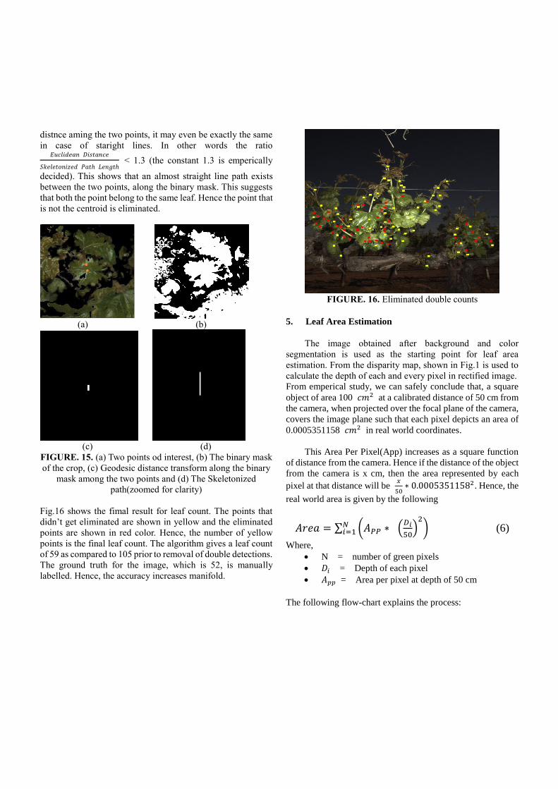
Fig.16 shows the fimal result for leaf count. The points that

didn’t get eliminated are shown in yellow and the eliminated

points are shown in red color. Hence, the number of yellow

points is the final leaf count. The algorithm gives a leaf count

of 59 as compared to 105 prior to removal of double detections.

The ground truth for the image, which is 52, is manually

labelled. Hence, the accuracy increases manifold.

FIGURE. 16. Eliminated double counts

5. Leaf Area Estimation

The image obtained after background and color

segmentation is used as the starting point for leaf area

estimation. From the disparity map, shown in Fig.1 is used to

calculate the depth of each and every pixel in rectified image.

From emperical study, we can safely conclude that, a square

object of area 100 𝑐𝑚2 at a calibrated distance of 50 cm from

the camera, when projected over the focal plane of the camera,

covers the image plane such that each pixel depicts an area of

0.0005351158 𝑐𝑚2 in real world coordinates.

This Area Per Pixel(App) increases as a square function

of distance from the camera. Hence if the distance of the object

from the camera is x cm, then the area represented by each

pixel at that distance will be 𝑥

50∗ 0.00053511582. Hence, the

real world area is given by the following

𝐴𝑟𝑒𝑎 = ∑ (𝐴𝑃𝑃 ∗ (𝐷𝑖

50)

2

)𝑁𝑖=1 (6)

Where,

• N = number of green pixels

• 𝐷𝑖 = Depth of each pixel

• 𝐴𝑝𝑝 = Area per pixel at depth of 50 cm

The following flow-chart explains the process:

(a) (b)

(d) (c)

0.2518 sq. m.

FIGURE. 17. Leaf Area Estimation flow-chart (a) Rectified

image, (b) Disparity Map, (c) Median filter application for

smoothening and (d) Image for area calculation

6. Results and discussion

Our imaging system consisting of a pair of RGB stereo

cameras and a pair of flashes is setup to optimize low motion

blur, capture increased depth-of-focus, and uses low

illumination power for fast-recycle times permitting high-

frame rates. This camera and illumination design maintains

high image quality at high vehicle velocities and enables

deployment on large scales. The imaging system is mounted

onto the side of the farm vehicle facing the fruit wall.

Depending on the size of the fruit zone a distance of 0.9 to

1.5m is maintained between the imaging system and the fruit

zone. The farm vehicle was driven at 1.5m/s through each row

and the images were captured at 5Hz.

The datasets were collected from different vineyards

across California. In each field calibration tags were put up

randomly in 10 rows and for 2 vines in each of the selected

rows. For shoot count estimation the ground truth was

measured on these rows manually by 2 people. Whereas, for

leaf area measurement the sensor data collected from a PAR

sensor was used as ground truth. The sensor values were

regularly sampled from start to end of a tag. Canopy light

penetration as well as ambient light data were recorded. These

values were used to find the correlation between the value

1 −𝐶𝑎𝑛𝑜𝑝𝑦 𝑙𝑖𝑔ℎ𝑡 𝑝𝑒𝑛𝑒𝑡𝑟𝑎𝑡𝑖𝑜𝑛

𝐴𝑚𝑏𝑖𝑒𝑛𝑡 𝑙𝑖𝑔ℎ𝑡 and algorithm output.

For testing the accuracy of leaf count estimation

algorithm, 32 images from a dataset containing the images of

Flame Seedless vines were randomly selected. These images

were hand labelled for marking and counting visible leaves in

the images.

Fig.19 and Fig.20 show the linear regression curves for

leaf count estimation and leaf area estimation respectively. The

correlation coefficient for leaf count estimation is 0.798 and

that for leaf area estimation is 0.69. The performance of the

system for shoot count estimation can be analyzed by the F1

score given in table 1. 25 images were randomly picked and

the visual shoot count in the images was done manually to

obtain the F1 score.

Precision Recall F1

Score

0.86 0.84 0.85

Table 1. Precision recall and F1 score

Each vine has an average length of 14 feet. Which then

converts to 4.2672 meters. Thus this helps to get ground truth

shoot count per meter for each of the vine. Then visual counts

for these images covering calibration vines was divided by

difference of real world x coordinate values obtained from the

disparity map at both the ends of calibration plots to get visual

shoot count per meter. To find the correlation between visual shoot count per meter

and ground truth shoot count per meter, we use Pearson’s

correlation. Correlation value was calculated to be 0.88. The

correlation graph is described in figure 18.

FIGURE 18 Correlation graph for ground truth shoot count per meter vs

algorithmically calculated shoot count per meter

FIGURE. 19 Linear Regression Curve for Leaf Count Estimation

FIGURE. 20 Linear Regression Curve for Leaf Area Estimation

7. Conclusion

It has been known that shoot density plays an important

role in grower decision making process regarding storage,

shipment, crop management and market price. Thus if there

exists an algorithm that can accurately estimate this parameter,

it can add economic value to the vineyard industry.

The quantitative analysis shows that there exists a

correlation between the visual shoot count per meter and the

actual shoot count per meter. The algorithm is validated by a

high F1 score of 0.85 and the existence of correlation between

visual count and ground truth can be validated by the

correlation coefficient value of 0.88. And for leaf area analysis,

it can be deduced that, there exists a correlation between the

PAR sensor data and estimated leaf area. The low value of the

R1 correlation coefficient might be attributed to the variance

in PAR data collection and vine image collection. Further

study is required to resolve this discrepancy. The work also

shows that the leaf count estimation algorithm has a correlation

coefficient of 0.798, with the manually ground truthed images.

The future work would estimate the correlation between the

total number of leaves counted in a vine and the algorithm

output.

8. Acknowledgement

This work is supported in part by the US

Department of Agriculture under grant number 2015-

51181-24393 and the National Grape and Wine

Initiative info@ngwi.org. The authors would like to

thank the following people who assisted in collecting the

data for this paper; Maha Afifi, Franka Gabler and Kaan

Kurtural and his lab at UC Davis.

References

[1] Z. Pothen and S. Nuske. “Texture-based fruit detection

via images using the smooth patterns on the fruit”. In

Proceedings of the IEEE International Conference on

Robotics and Automation, May 2016.

[2] Stephen Nuske, Kyle Wilshusen, Supreeth Achar, Luke

Yoder, Srinivasa Narasimhan, and Sanjiv Singh.

“Automated visual yield estimation in vineyards”.

Journal of Field Robotics, 31(5):837-- 860, September

2014.

[3] K.Ma College of Biosystems Engineering and Food

Science, Zhejiang University, “A Survey of Stem

Detection Algorithms and A New Algorithm Based on

Monte Carlo Method” Neural networks 6.6 (1993): 801-

806.

[4] Hung, Chia-Che, et al. "Orchard fruit segmentation using

multi-spectral feature learning." Intelligent Robots and

Systems (IROS), 2013 IEEE/RSJ International

Conference on. IEEE, 2013.

[5] Ruiz L A, Molto E, Juste F, et al. Location and

characterization of the stem-calyx area on oranges by

computer vision [J]. Journal of agricultural engineering

research, 1996, 64(3): 165-172.

[6] Paproki, Anthony, et al. "Automated 3D segmentation

and analysis of cotton plants." Digital Image Computing

Techniques and Applications (DICTA), 2011

International Conference on. IEEE, 2011.

[7] Alejandro F. Frangi, Wiro J. Niessen, Koen L. Vincken

and Max A. Viergever. Multiscale vessel enhancement

filtering. Lecture Notes in computer Science, 1496:

130—137, October 1998.

[8] Richard O. Duda and Peter E. Hart. Use of the Hough

Transformation to detect lines and curves in pictures.

Communications of the ACM, 15:11—15, January 1972.

[9] Dunn, G., & Martin, S. (2004). Yield prediction from

digital image analysis: A technique with potential for

vineyard assessments prior to harvest. Australian Journal

of Grape and Wine Research, 10: pp 196198.

[10] Rabatel, G, and C Guizard. (2007). Grape berry

calibration by computer vision using elliptical model

fitting. European Conference on Precision Agriculture, 6:

pp. 581- 587.

[11] Alenyà, G., et al. "Leaf segmentation from ToF data for

robotized plant probing." IEEE Robotics &Automation

Magazine (2012).

[12] Xia, Chunlei, et al. "In situ 3d segmentation of individual

plant leaves using a rgb-d camera for agricultural

automation." Sensors 15.8 (2015): 20463-20479.

[13] Li, Chunming, Jundong Liu, and Martin D. Fox.

"Segmentation of edge preserving gradient vector flow:

an approach toward automatically initializing and

splitting of snakes." 2005 IEEE Computer Society

Conference on Computer Vision and Pattern Recognition

(CVPR'05). Vol. 1. IEEE, 2005.

[14] Giuffrida, Mario Valerio, Massimo Minervini, and

Sotirios A. Tsaftaris. "Learning to count leaves in rosette

plants." (2016): 1-1.

[15] A. Coates, A. Arbor, and A. Y. Ng. An analysis of single-

layer networks in unsupervised feature learning.

International Conference on Artificial Intelligence and

Statistics, pages 215–223, 2011.

[16] C. Elkan. Using the triangle inequality to accelerate k-

means. In International Conference on Machine

Learning, pages 147–153, 2003.

[17] Xia, C., Lee, J. M., Li, Y., Song, Y. H., Chung, B. K., &

Chon, T. S. (2013). Plant leaf detection using

modified active shape models. Biosystems

engineering, 116(1), 23-35.

[18] Diago MP, Correa C, Millán B, Barreiro P, Valero C,

Tardaguila J. Grapevine yield and leaf area estimation

using supervised classification methodology on RGB

images taken under field conditions. Sensors. 2012 Dec

12;12(12):16988-7006.

[19] Knyazikhin, Y.; Martonchik, J.V.; Diner, D.J.; Myneni,

R.B.; Verstraete, M.; Pinty, B.; Gobron, N. Estimation of

vegetation canopy leaf area index and fraction of

absorbed photosynthetically active radiation from

atmosphere-corrected MISR data. J. Geophys. Res.

Atmos. 1998, 103, 32239-32256.

[20] Haboudane D, Miller JR, Tremblay N, Pattey

E,Vigneault P. Estimation of Leaf Area Index using

Ground spectral measurements over Agriculture crops:

Prediction capability assessment of optical indices. Can.

J. Remote Sens. 2004;23:143-62.

[21] Mohammed Amean, Z., et al. "Automatic plant

branch segmentation and classification using vesselness

measure." Proceedings of the Australasian Conference

on Robotics and Automation (ACRA 2013). Australasian

Robotics and Automation Association, 2013.

[22] Fit an Ellipse to a Region of Interest (September 22,

2016). Retrieved from :

http://www.idlcoyote.com/ip_tips/fit_ellipse.html