V(2.0) 2/12/04 For submission to Bulletin Seismological Society of America

1

Earthquake Simulation by Restricted Random WalksSteven N. Ward

Institute of Geophysics and Planetary Physics

University of California, Santa Cruz

Abstract. This article simulates earthquake slip

distributions as restricted random walks. Random walks

offer several unifying insights into earthquake behaviors

that physically-based simulations do not. With properly

tailored variables, random walks generate observed

power law rates of earthquake number versus

earthquake magnitude (the Gutenberg-Richter relation).

Curiously b-value, the slope of this distribution, not

only fixes the ratio of small to law events but it also

dictates diverse earthquake scaling laws such as mean

slip versus fault length and moment versus mean slip.

Moreover, b-value determines the overall shape and

roughness of earthquake ruptures. For example, mean

random walk quakes with b=-1/2 have elliptical slip

distributions characteristic of a uniform stress drop on a

crack. Random walk earthquake simulators, tuned by

comparison with field data, provide improved bases for

statistical inference of earthquake behavior and hazard.

1. Introduction.

Imagine hiking the trace of a new

earthquake rupture and measuring surface slip

offsets at many points along the fault strike

(see Figure 1, for examples). This mapping

exercise may be akin to a random walk in the

sense that the measured offset at position n

gives scant hint as to whether the offset at

position n+1 will be larger or smaller.

Consider then, earthquake slip

functions u(n∆L) sampled at regular intervals

∆L as simulated in

u(n L) = u0 + u χi (0, σi )i=1

n

∑ (1)

Here, ∆u is some small slip value and the

χ(ν,σ) are unitless random variables with

mean ν and variance σ2. Random walk

"ruptures" (1) start with u0 = u and run a

distance L=N∆L to where u(N L) ≤ 0

Figure 1. Measured dextral displacement along thesurface fault trace of the Sakarya Segment, M7.4 Ismit,Turkey earthquake of August 17, 1999 (Barka et al.,2002) and the M7.1 Duzce, Turkey earthquake ofNovember 12, 1999 (Akyuz et al., 2002).

Figure 2. Sketch of an earthquake rupture simulatedby a restricted random walk. The rupture starts at l=0with slip ∆u and runs down strike taking randomfluctuations in slip until u(L) first falls to zero orbelow.

2

(Figure 2). The rupture terminates there and

the earthquake is finished. Random walks like

these, that terminate at a barrier are labeled

restricted or absorbing.

The extent to which simulation (1)

might represent earthquakes hinges upon the

selection of the random variables. In a leap of

faith, suppose that the synthetic ruptures could

indeed be made to reproduce many earthquake

behaviors. If so, then random walks would, at

the least, provide simple statistical bases for

testing rupture hypotheses. Strong leapers

might even imagine random walks leading to

insights into earthquake behavior that physics-

based rupture simulations obscure in curtains

of complexity.

2. Walk Statistics.

Unrestricted Walks Reaching Length L.

Envision initially, unrestricted random walks

with u0=0 that run length L as shown in Figure

3. Let Pu( L )(u) be the probability of u(L)

falling between u and u+ u. If the random

variables χn are well enough behaved such that

the central limit theorem holds, then for large L

Pu( L )(u) would be normally distributed with

zero mean and variance σ2(L)

Pu( L )(u) = u2

∂∂u

erf u2σ (L )( ) (2)

The erf(x) here is the integrated Gaussian or

error function (see Appendix A). The variance

of unrestricted walk heights at L is defined by

σ 2(L) = u−1 u2

−∞

∞∫ Pu(L )(u)du

= L−1 σ2 (l)0

L

∫ dl (3)

where ∆σ is the variance increment along the

path from 0 to L. For independent χn in (1)

σ2 (n L < l < (n + 1) L) = u2σn2

and

σ 2(L) = u2 σn2

n=1

N=L / L

∑ (4)

Restricted Walks Reaching Length L. When the

Figure 4. Probability distribution Pu( L )(u, u) of u(L)

from many restricted walks that reach L (eq 5).

Pu( L )(u, u) is one-sided with positive mean.

Figure 3. Sketch of several unrestricted walks based on

the same random variables as the restricted walk in

Figure 2. Pu( L )(u) , the probability distribution of u at L

from many trials, is generally Gaussian for long walks.

3

walk is restricted to positive offsets only and

u0=∆u, then the probability of u(L) falling

between u and u+∆u becomes

Pu (L )(u, u) =

Pu (L )(u − u) − Pu (L ) (u + u)

= u

2

∂∂u

erf u+ u2σ (L )( ) − erf u− u

2σ (L )( )

(5)

I sketch equation (5) toward the right in Figure

4. Integrating Pu (L )(u, u) over all values u,

gives the probability that the restricted walk

runs a distance L or greater

P> ( u, L) = u−1

0

∞

∫ Pu( L )(u, u)du

= erf u

2σ (L )( ) ≈ 2

πu

σ(L)

(6)

The probability that the restricted walk

actually ends between L and L+∆L

P( u, L) = L∂P>( u, L)

∂L

= 2π

u Lσ2(L)

e

− u2

2σ2 (L) ∂σ(L)∂L

≈ 2π

u Lσ2(L)

∂σ(L)∂L

≈ P> ( u,L)u L

σ( L)∂σ(L)

∂L

(7)

is just the fraction that reach distance L times a

positive number less than one. In the restricted

walk, the expected value and variance of the

heights at L areE[u(L)] =

u erf u

2σ (L)( )

−1

≈ π2

σ(L) (8a)

and

Var[u(L)] = σ2 (L) + u2

+ 2π

σ(L)e− u

2

2σ2 (L) E[u(L)] − E[u(L)]2

≈ (2 − π / 2 )σ2 (L) = 0.43σ 2( L)

(8b)

The approximate versions of (6-8) hold for

long ruptures where σ(L)>>∆u. Restricted

walks have a non-zero mean value with a

spread in offsets about half as large as

unrestricted walks of equal length.

Random walk theory (6) predicts an

inverse relationship between the length-

survivability of earthquake ruptures and the

degree to which slip varies along strike. To my

knowledge, physics-based models of

earthquake rupture have not made such a

prediction. In particular, random walk quakes

with large step-to-step variations have less

chance of making long ruptures than do

quakes with small step-to-step variations. Bear

in mind, that the variation in earthquake slip

along strike, σ2(L) is field-measurable, so

means exist to test and tune the simulator. Slip

variation forms a common thread through all

predictions below.

Restricted Walks Terminating Length L.

Consider finally restricted random walks that

terminate at L (Figure 5). These walks

4

resemble earthquake ruptures of length L and I

label their offset along strike uL(l). Because the

offset vanishes at both ends of the rupture, the

variance σ L2 (l < L) of uL(l) increases like (4)

initially, but then tapers to zero at L

σ L2 (l) =

σ 2(l)

σ 2(L)σ2 (L ) − σ2(l)[ ] (9)

From (8a), the expected value of slip at

distance l in such ruptures would be

E[uL (l)] ≈ π2

σ L (l) (10)

Thus, the mean slip of all earthquakes of

length L depends on along-strike slip

variability like

U ( L) = π / 2

Lσ(L)×

σ(l) σ2 (L) − σ2 (l)[ ]1 / 2

0

L∫ dl

(11)

Seismologists have particular interest in the

seismic moment of earthquakes

Mo = µWLU (12)

where µ is the elastic rigidity of the crust, U isthe mean slip in the event, and W is the down

dip (into the Earth) width of ruptures in the

region of interest. [W is assumed constant

here.] From (11) and (12), the mean moment

in all quakes terminating at L would be

M 0( L) = µWLU ( L) (13)

Once our simulation specifies slip variability

σ2(L), then M 0( L) can be inverted to provide

L (M0 ), the mean rupture length needed to

generate a given seismic moment. Back

substitution of L (M0 ) into (6) then provides

the probability that simulated earthquakes

exceed a given moment

P> ( u, M0 ) ≈ 2π

uσ(L (M0 ))

(14)

3. Application to earthquakes.

Predicted Rate Distribution. What does this

theory really have to do with earthquakes?

Suppose that I find a set of random variables

χn such that standard deviation of slip along

the unrestricted walk (4) grows like

σ(l) ≈ u(l / L) q (15)

Evaluating integral (11) then, provides the

mean slip in quakes of length L

Figure 5. Points of restricted walks that terminate at L.

This class of random walks resembles earthquake

ruptures of length L. The predicted statistics of slip

variation along strike in these ruptures provide a key

field test for application to real earthquakes.

5

U ( L) = uπ8

π2q

(1+ q2q

)

(1 + 4q

2q)

LL

q

= uK (q)( L / L)q

(16)

Placing (16) into (13) and inverting for the

mean rupture length for quakes with moment

M0, I find

L (M0 ) = LM0

(µ uW L)K(q)

1

q+1

= LM0

M0K(q)

1

q+1

(17)

and (15) gives

σ(L (M0 )) ≈ uM0

M0K(q)

q

q+1 (18)

with M0 = µ uW L. From (14) the

probability that a quake grows to moment Mo

or greater is

P> (M0 ) = 2π

M0K(q)[ ]q /(q+1)M0

−q /(q +1)

(19)

Finally, using the moment-magnitude relation

Mw=(2/3)[log(M0)-9.05], I write (19) as

log N>(MW ) = log N> (MWmin )

+[− 32

q(1+ q)

]( MW − MWmin )

(20)

Equation (20) specifies a power-law

distribution in the rate of quakes of magnitude

greater than Mw. That is, random walk

simulations (1) with variance (15) produce

earthquakes that obey the Gutenberg Richter

relation with

b = − 32

q(1+ q)

or q = −2b

3 + 2b (21)

Equation (21), the first clear tie of random

walks with earthquake behaviors, offers initial

justification for that leap in Section 1.

Predicted Scaling Laws. From (16) and (13)

other earthquake scaling laws too can be

written in terms of b-value

U ( L) = uK(q)LL

−2b

3+2b = K(q)σ( L)

(22)

M 0( L) = M0 K(q)LL

3

3+2b (23)

U ( M0 ) = uK(q)3+ 2b

3 M 0M0

−2b

3 (24)

Remarkably, b-value not only dictates the ratio

of large to small earthquakes, but it also fixes

the slope of many of their scaling laws. I know

of no physics-based model of earthquake

rupture that makes this link. In fact, random

walk theory predicts that not only are slopes of

the scaling laws interrelated but so are the

leading constants. (K(q) is given in Table 1.)

Reproduction of observed scaling law slopes

and their constants would be a strong

endorsement of random walk simulations.

6

For earthquakes in bulk, a b-value of -1

is nearly universal. Random walk quakes with

b=-1 scale like

U ∝ L2 ; M 0 ∝ L3 and U ∝ M02 / 3 (25)

There is no reason however, that the simulator

need reproduce bulk quake rates especially if it

is intended to model events on a particular

fault. Earthquakes restricted to the vicinity of a

particular fault can have b-values considerably

greater than -1 because isolated faults often

produce many similar-sized events. Table 1

shows that seismic sources that vary in b-value

by only a few tenths generate earthquakes that

scale quite differently from (25). A

dependence of scaling laws on the underlying

b-value of the earthquake source could be a

core confusion in quantifying earthquake

behavior. Comparing rupture statistics from

mixed populations of different b-valued

sources would create a wide variability in

observed earthquake scaling.

Predicted Slip Function Features. From (9),

(10) and (15) the mean shape of earthquake

slip functions in ruptures of length L is

E[uL (l)] = 2U peakl q

L2q L2q − l2q[ ]1 / 2(26)

with

U peak = uπ8

LL

q

(27)

Amazingly, random walk theory says that b-

value also controls the mean shape of

earthquake slip functions. Figure 6 (left) plots

(26) for b=-1/4 to b=-1. Note that the mean

slip from b=-1/2 sources

Figure 6. (Left) Mean shape of earthquake slip functions

versus b-value of the source. (Center) 2-D Stress drops

associated with the mean slip functions. (Right) Typical

realizations of ruptures with the given b-value.

q b U(L) U(M) M(L) K(q) U

peak( L)

U ( L)

Upeak

field (L)

U ( L)2 -1 u ∝ L2 u ∝ M0

2 / 3 M 0 ∝ L3 0.300 2.08 3.52

3/2 -0.9 u ∝ L3 / 2 u ∝ M00.6 M 0 ∝ L5 / 2 0.351 1.78 3.00

1 -3/4 u ∝ L1 u ∝ M01 / 2 M 0 ∝ L2 0.417 1.50 2.52

1/2 -1/2 u ∝ L1 / 2 u ∝ M01 / 3 M 0 ∝ L3 / 2 0.492 1.27 2.13

1/5 -1/4 u ∝ L1 / 5 u ∝ M01 / 6 M 0 ∝ L6 / 5 0.477 1.31 2.20

Table 1. Earthquake Scaling Laws versus b-value as predicted from random walk theory.

7

E[uL (l)] =2U peak

Ll(L − l)[ ]1 / 2 (28)

follows exactly the elliptical shape expected

from a uniform stress drop of

τ = −µU peak

L (29)

over a 2-D shear crack of length L (middle

Figure 6). Equation (29) is another indication

that fundamental relationships exist between

random walks and earthquake physics. As b-

value decreases to b=-1, the crack-like slip

functions evolve to a dogtail/rainbow

appearance (Ward, 1997). In these ruptures,

stress drops over the concave down part of the

rupture (the rainbow) while stress increases

over the concave up part (the dogtail). Both

dogtail/rainbow and elliptical slip functions

are observed frequently in the field. Note too

that ruptures from b<-1/2 sources are

intrinsically skewed in walks (15). Skewness

of slip functions is a field measurable quantity

and this prediction too should be testable.

From (22), the peak mean slip to mean

slip ratio

U peak (L)

U (L)

=

π8

K −1(q) (30)

also depends on b-value but it is independent

of the length of rupture. Peak slip to mean slip

ratio might be thought of as an unrecognized

earthquake scaling law. Random walk theory

says that slip functions from low b-value

earthquake sources should be more "peaky"

than those from higher b-value sources. As

mentioned above, high b-value sources

produce a larger proportion of characteristic

earthquakes than do low b-value sources.

Reduced slip variability for more characteristic

sources makes sense. Peak mean slip to mean

slip ratio (30) goes from 1.3 to 2.1 as b value

decreases from -1/2 to -1. Equation (30)

however must underestimate field-measured

peak slip to mean slip ratios. Smooth shapes

(26) represent the slip averaged over all

quakes of length L. Individual rupture events

randomly perturb these shapes (see far right

Figure 6) and will certainly peak out higher.

From (8b) and (10) the variance in mean peak

height is

Var[U peak ] = (2 − π / 2 )22π

U peak2

Likely field-measured peak slip might exceed

the mean value by 2 standard deviations

U peakfield ≈ 1 + 2 × (2 − π / 2 )

2π

U peak

= 1.68U peak

so a better, metric of slip variability might be

Upeak

field (L)

U ( L)

= 1.68 × π

8K −1(q) (31)

Equation (31) goes from 2.2 to 3.5 as b value

increases from -1/2 to -1. Predictions of slip

function "peakyness" as measured by the ratio

of peak slip to mean are field-testable.

8

We have seen now that random walk

theory makes many specific predictions about

the behaviors of earthquake ruptures. The b-

value controls not only the scaling law

constants but it also affects the "look and feel"

of the slip distribution. I believe that correctly

mimicking the look and feel of earthquake

ruptures is critically important both in the

tuning of the simulator and in assuring its

practical use.

4. Design of the Walks- Numerical Results.

Basic Walk. The analytical results above

provide a good foundation for what to expect

from random walk simulations. Let's now

compute (1) to visualize slip functions and to

verify the predictions. As a first step, I fix step

distance along strike (∆L=100 m), rigidity (µ=

3x1010 Nm), and down-dip fault width

(W=15,000 m). Secondly, I need to find a set

of zero mean random variables χn such that the

summed variance along the walk (5) equals

(15). Many random variables have equal

variances and zero mean and all should make

quakes that satisfy the scaling relations (22-

24). The choice may however, influence the

look and feel of the slip functions in subtle

ways. The simplest approach assumes that χn

are normally distributed with zero mean but

with a variance that increases with distance

l=n L along strike as

χn = N(0, 2qn (2 q−1 ) / 2) (32)

For uncorrelated χn, the variance along the

unrestricted walk (4) is

Figure 7. (Left) Features of restricted random walk quakes with b=-1, -3/4, -1/2 and -1/4. The solid linessummarize 1 million random walk quakes. The dashed lines are expected scaling laws (22-24). (Panel A)Number versus Magnitude The slope of these curves is the b-value. (Panel B) Mean slip versus rupture length.(Panel C) Mean slip versus Moment. (Panel D) Mean Length versus Moment. (Right) Features of restrictedrandom walk quakes with b=-1. Inclined dashed lines in the bottom panels are the Slip versus Moment relationof Wells and Coppersmith (1994) and the Length versus Moment findings of Kagan (2002). Flat dashed line inPanel C graphs peak height/mean height ratio versus earthquake size.

9

σ 2(l = n L) = 2q u2 i2q−1

i=1

n

∑

≈ u2 (l / L)2q

(33)

as needed by (15). The only free parameters

remaining in the simulation are b-value and

slip increment ∆u.

Figure 7 (left) summarizes statistics of

one million random walks with b= -1/4, -1/2, -

3/4 and -1. I adjusted slip increment ∆u in each

case to produce about 1-meter of mean slip on

faults of 80 km length. The dashed lines are

the predicted scaling laws (22)-(24) and the

expected power-law behaviors are all well

matched.

The right half of Figure 7 isolates the

behaviors for b=-1 sources. The inclined

dashed lines in the bottom two panels graph

the independently observed earthquake scaling

relations of Wells and Coppersmith (1994)

logU (m) = 0 . 6 l o gM0 (Nm) −11.75 (35)

and Kagan (2002)

log L(km) = 0.315log M0 ( Nm) − 4.27 (36)

Sources with b=-1 reproduce both of these

relations in slope and intercept. The flat

dashed line in Panel C (right) plots the peak

height to mean height ratio of the simulated

ruptures, binned as a function of earthquake

moment. As expected, the peak height to mean

height ratio depends on b-value but is

independent of earthquake size. Computed

ratios for b= -1/4, -1/2, -3/4 and -1 are 2.0, 2.0,

2.3 and 3.2 -- just a bit less than expected from

(31).

Figure 8 plots a selection of the

random walk ruptures tabulated in Figure 7.

The quakes have magnitude 7 to 7.5 drawn

from b= -1/2, -3/4 and -1 sources. You can see

that ruptures from lower b-value sources

(center and right) are progressively more

peaky and skewed than those from b=-1/2

sources. For comparison, the bottom row of

Figure 8 plots the observed slip distributions

from Figure 1 scaled somewhat in horizontal

and vertical dimensions. Although the

Figure 8. Earthquake ruptures 7.0<Mw<7.5 as simulatedby a basic random walk (1) with (32) with b=-1/2, -3/4and -1.

10

simulator has yet to be tuned in any way, many

of the synthetic slip functions could be

mistaken for real.

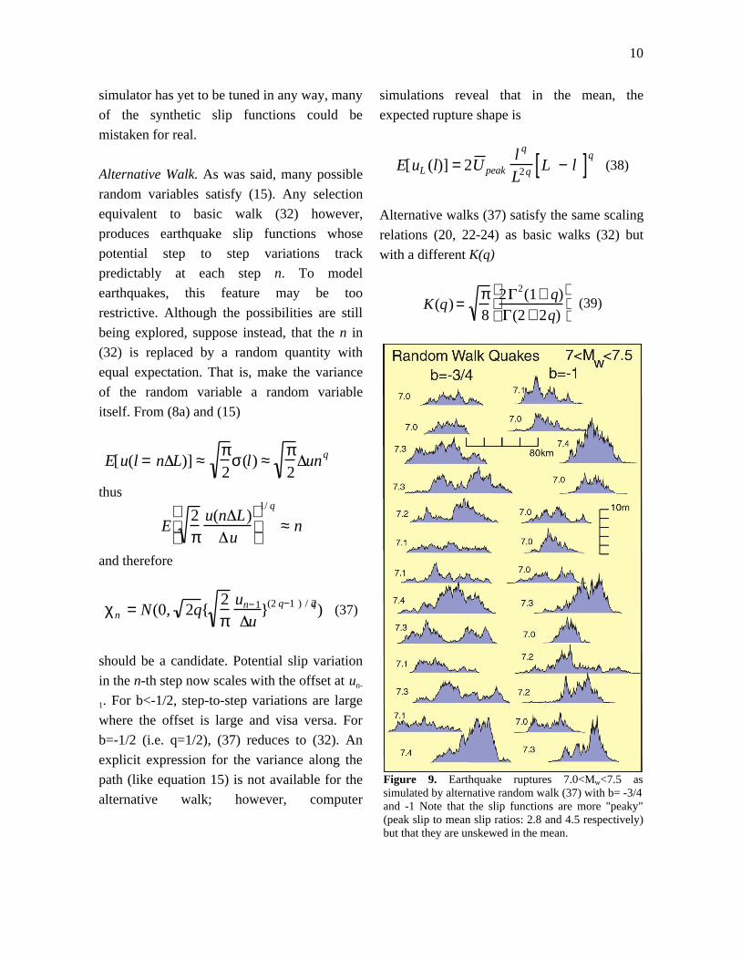
Alternative Walk. As was said, many possible

random variables satisfy (15). Any selection

equivalent to basic walk (32) however,

produces earthquake slip functions whose

potential step to step variations track

predictably at each step n. To model

earthquakes, this feature may be too

restrictive. Although the possibilities are still

being explored, suppose instead, that the n in

(32) is replaced by a random quantity with

equal expectation. That is, make the variance

of the random variable a random variable

itself. From (8a) and (15)

E[u(l = n L)] ≈ π2

σ(l) ≈ π2

unq

thus

E2π

u(n L)u

1/ q

≈ n

and therefore

χn = N(0, 2q{2π

un−1

u}(2 q−1 ) / 2q) (37)

should be a candidate. Potential slip variation

in the n-th step now scales with the offset at un-

1. For b<-1/2, step-to-step variations are large

where the offset is large and visa versa. For

b=-1/2 (i.e. q=1/2), (37) reduces to (32). An

explicit expression for the variance along the

path (like equation 15) is not available for the

alternative walk; however, computer

simulations reveal that in the mean, the

expected rupture shape is

E[uL (l)] = 2U peakl q

L2q L − l[ ]q (38)

Alternative walks (37) satisfy the same scaling

relations (20, 22-24) as basic walks (32) but

with a different K(q)

K(q) = π8

2 2(1+ q)(2 + 2q)

(39)

Figure 9. Earthquake ruptures 7.0<Mw<7.5 assimulated by alternative random walk (37) with b= -3/4and -1 Note that the slip functions are more "peaky"(peak slip to mean slip ratios: 2.8 and 4.5 respectively)but that they are unskewed in the mean.

11

More importantly, because slip (hence slip

variance) tapers to zero at both ends of the

rupture, offsets (38) are unskewed for any b-

value. This may have advantage when fitting

real data.

Figure 9 shows a selection random

walk earthquakes of magnitude 7 to 7.5 from

sources with b= -3/4 and -1 using alternative

(37). While these walks are slightly peakier

than those in Figure 8, they look realistic. In

tuning simulations to fit real earthquake

observations, blends of the basic and

alternative walks might be most suitable.

5. Application: Paleoseismic RuptureCorrelation

Even if randomness is a stand in for

unknown physics, restricted walk ruptures

seem capable of mimicking observed

earthquake rates, scaling properties, and "look

and feel". Granted this, what purpose can the

simulations serve?

A typical situation in paleoseismic

work is finding that: 1) Earthquake A broke

through Site A D1±∆1 years ago; 2) that

Earthquake B broke through Site B D2±∆2

years ago; and that 3) the age limits D1±∆1 and

D2±∆2 overlap. The paleoseismic correlation

problem amounts to deciding whether rupture

events A and B are distinct or are one in the

same. The decision often strongly influences

earthquake hazard estimates.

In the past, the correlation decision

largely hinged on the probability that the age

dates were in fact equal. Recently, Biasi and

Weldon (2004) proposed a means to improve

correlations by blending age overlap

probabilities with rupture survival

probabilities. If event offset U can be

measured at either Site 1 or 2 and the distance

between them is known, then a properly tuned

random walk simulator can assist in the

decision.

The statistical simulator views

earthquake correlation as a Gambler's Ruin

problem where slip plays the role of money

and each km along strike plays the role of a

dice toss. The simulator tells us the

probability that the rupture will reach from

site A to Site B before its slip is played out.

For instance, a paleo earthquake rupture is

found to have two meters of slip at

Wrightwood California. What is the

probability that slip runs to zero before the

rupture covers the 30 km distance south to

Pallet Creek?

Computationally, rupture survival

calculations use the simulator parameters (∆u,

∆L, W, b or q, and χn) tuned to the fault in

question. The only difference being that u0 in

(1) is set to the slip value U>>∆u observed at

one of the paleoseismic sites. After many

simulations, the fraction of ruptures that reach

distance L are tabulated. Alternatively, if the

variance accumulation in the walk σ(L) is

specified, then equation (6) gives the survival

probability analytically. For the basic walk,

the rupture survival curves are

P> (U,L) = erf U

2σ (L )( )= erf U

2 u (L / L)q

= erf K (q)

2

U

U (L )( ) (40)

12

Figure 10 plots rupture survival probabilities

for the basic walk with b=-1 for U=0.1, 0.5, 1,

2, and 4 meters. For instance, suppose the

distance between the two paleoseismic sites is

L=25 km, then a rupture with a 10 cm offset at

Site A has only 20% chance of reaching Site

B. A rupture with a 1/2 m offset however has

a 85% chance of breaking both sites. The last

of (40) interprets rupture survival in terms of

the mean slip U ( L) in quakes of length L. If

the offset U at Site A is large compared to

U ( L) , then the rupture will most likely reach

the distance L to Site B. No need to be a

rocket scientist to understand this conclusion.

Figure 11 plots rupture survival curves

for the alternate walk with b=-1. For L=25

km, a rupture with a 10 (50) cm offset at Site

A has only 10% (35%) chance of reaching

Site B. The added peakiness in the alternative

walk reduces survival probability by about

half.

6. Conclusions

Many seismologists are working to construct

physically-based earthquake simulators.

Physical simulators hold considerable appeal,

however they may become so complex that

much of the modeling effort is expended in

finding a physical basis for essentially random

behavior. If certain aspects of earthquake

behaviors are random to the extent that real

data can constrain them, then a more practical

approach may be to embrace the randomness

whatever its physical origin.

This article begins to develop and to apply

random walk rupture simulations to

earthquake issues and to assemble a catalog of

observed earthquake slip functions with which

to test the simulator. Statistical simulators like

these, are intended to complement physical

simulators in those applications where they

may be better suited. Once calibrated against

observed slip functions, statistical simulators

Figure 11. Rupture survivability curves for thealternate walk with b=-1 (right column Figure 9).Survival probability is a bit less for these more peakyruptures than those of Figure 10.

Figure 10. Rupture survivability curves for the basicwalk with b=-1 (right column Figure 8). Curves showthe probability that a rupture with offset U (0.1m to4m) at Site A reaches Site B given the distance Lbetween them.

13

can serve as a scientific tool to aid in the

understanding of other characteristics of

earthquakes that are not easily, or not yet,

measured.

Restricted random walk (1) with standard

deviation (6) generates earthquake sets that

reproduce observed power law rates of

earthquake number versus magnitude as well

as diverse earthquake scaling laws such as

mean slip versus fault length and moment

versus mean slip. By tying together earthquake

rates, earthquake scaling laws, and earthquake

slip shape and variation through b-value,

humble random walks hint at a unified theory

of earthquake behavior.

References.

Akyuz, H. S. et. al. 2002. Surface rupture and slip

distribution of the 12 November 1999 Duzce

Earthquake (M7.1), North Anatolian Fault,

Bolu, Turkey, Bull. Seism. Soc. Am., 92, 61-66.

Barka, A., et. al., 2002. Surface rupture and slip

distribution of the 17 August 1999, Ismit

Earthquake (M7.4) North Anatolian Fault, Bull.

Seism. Soc. Am., 92, 43-61.

Biasi G, and R. Weldon R., 2004. Estimating

surface rupture length and magnitude of

paleoearthquakes from point observations of

rupture displacement, (preprint, to be

submitted).

Kagan, Y. Y. 2002. Bull. Seism. Soc. Am., 92, 641-

655.

Ward, S. N., 1997. Dogtails versus Rainbows:

Synthetic earthquake rupture models as an aid

in interpreting geological data, Bull. Seism. Soc.

Am., 87, 1422-1441.

Wells, D.L. and K. J. Coppersmith, 1994. New

empirical relationships among magnitude,

rupture length, rupture width, rupture area, and

surface displacement, Bull. Seism. Soc. Am.,

84, 974-1002.

Appendices

A. Error FunctionThe error function erf(x) smoothly varies from

0 at x=0 to 1 at x=∞ (Figure A1). Also,

erf(1)=0.842, erf(2)=0.995, and erf(-x)=-

erf(x). For small x, .erf( x) ~2x / π .

B. Slip variability and rupture survivability

Random walk (1) with u0 = u can be

written as a sum or a product of terms

u n = u + u χ i (0, σi )i=1

n

∑ (A1)

= u 1 + uui -1

χi (0,σ i )

i=1

n

∏

= u 1 + χi (0,σ i u

u i -1

)

i=1

n

∏

= u χ i(1,σ i uu i-1

)i=1

n

∏ (A2)

The walk terminates at the i-th step when

Figure A1. The error function.

14

χ i (0,σi uu i -1

) < −1

If χ is normally distributed, the probability of

termination is

−∞

−1

∫ N (x : 0,σi u

u i -1

)dx

= 12

1 − erfu i-1

2σ i u

(A3)

For a given offset un-1, the larger the step to

step variability σi, the higher the chance of

termination. This association gives rise to the

inverse relation between slip variability and

rupture survivability characterized by b-value.