EBF3GLWingOpt: A Framework for Multidisciplinary Design

Optimization of Wings Using SpaRibs

Qiang Liu

Dissertation submitted to the Faculty of the Virginia Polytechnic Institute and State University in fulfillment of the requirements for the degree of

Doctor of Philosophy in

Engineering Mechanics

Rakesh K. Kapania (Committee Chair) Scott W. Case

Mark S. Cramer Muhammad R. Hajj Mayuresh J. Patil

June 05, 2014 Blacksburg, Virginia

Keywords: Structural Optimization, Global-local Optimization, Wing Optimization, Multidisciplinary Design Optimization, SpaRibs, Stiffened Panel Optimization

Copyright 2014, Qiang Liu

EBF3GLWingOpt: A Framework for Multidisciplinary Design

Optimization of Wings Using SpaRibs

Qiang Liu

ABSTRACT

A global/local framework for multidisciplinary optimization of generalized aircraft wing

structure has been developed. The concept of curvilinear stiffening members (spars, ribs and

stiffeners) has been applied in the optimization of a wing structure. A global wing optimization

framework EBF3WingOpt, which integrates the static aeroelastic, flutter and buckling analysis,

has been implemented for exploiting the optimal design at the wing level. The wing internal

structure is optimized using curvilinear spars and ribs (SpaRibs). A two-step optimization

approach, which consists of topology optimization with shape design variables and size

optimization with thickness design variables, is implemented in EBF3WingOpt. A local panel

optimization framework EBF3PanelOpt, which includes stress and buckling evaluation criteria,

is performed to optimize the local panels bordered by spars and ribs for further structural weight

saving. The local panel models are extracted from the global wing finite element model. The

boundary conditions are defined on the edges of local panels using the displacement fields

obtained from the global model analysis. The local panels are optimized to satisfy the stress and

buckling constraints. Stiffened panel with curvilinear stiffeners is implemented in the

iii

EBF3PanelOpt to improve the buckling resistance of the local panels. The optimization of

stiffened panels has been studied and integrated in the local panel optimization. The global wing

optimization EBF3WingOpt has been applied for the optimization of the wing structure of the

Boeing N+2 supersonic transport wing and NASA common research model (CRM). The

optimization results have shown the advantage of curvilinear spars and ribs concept. The local

panel optimization EBF3PanelOpt is performed for the NASA CRM wing. The global-local

optimization framework EBF3GLWingOpt, which incorporates global wing optimization

module EBF3WingOpt and local panel optimization module EBF3PanelOpt, is developed using

MATLAB and Python programming to integrate several commercial software: MSC.PATRAN

for pre and post processing, MSC.NASTRAN for finite element analysis. An approximate

optimization method is developed for the stiffened panel optimization so as to reduce the

computational cost. The integrated global-local optimization approach has been applied to

subsonic NASA common research model (CRM) wing which proves the methodology’s

application scaling with medium fidelity FEM analysis. Both the global wing design variables

and local panel design variables are optimized to minimize the wing weight at an acceptable

computational cost.

iv

Dedication

This dissertation is dedicated to my beloved family 

for their endless love, invaluable guidance, relentless support and encouragement. 

v

Acknowledgements

I am grateful to all people who encouraged me and supported me throughout my life. I have a

number of individuals to thank for helping me to pursue my dream and

I would like to express my deepest gratitude to my supervisor, Professor Rakesh K. Kapania, for

his encouragement, patient guidance and support throughout my PhD research. Without him, I

would not have the opportunity of working with some of the greatest experts in aerospace

sciences. He was a true mentor and guided me along the path toward my doctorate. I cannot

thank him enough for all he taught me.

I would like to thank my dissertation committee members, Dr. Scott Case, Dr. Mark Cramer, Dr.

Muhammad R. Hajj, Dr. Mayuresh Patil, for their precious time, sharing their knowledge and

experience with me.

I would like to thank Karen M. Brown Taminger of NASA Langley Research Center, as the

technical monitor of the project funded under NASA’s Fundamental Subsonic Aeronautics

Program through a subcontract from the National Institute of Aerospace, Hampton, Virginia. I

would like to thank Carol D. Wieseman, Bret K. Stanford, James B. Moore, and Christine V.

Jutte of NASA Langley Research Center for substantial technical discussions and inputs. The

vi

original research on the SpaRibs concept was funded under the NASA’s Fundamental

Aeronautics Program for Supersonic Aircraft with Marcia Domack as the project monitor.

I would like to express my sincere thanks to Dr. Sameer B. Mulani. Discussing technical matters

with him is always a pleasure and an enriching experience. I would like to thank other members

in our research group, Dr. Davide Locatelli, Wei Zhao, Mohamed Jrad, and Shuvodeep De, for

their valuable help throughout my studies.

I would like to thank all my friends at Virginia Tech. My life in Blacksburg would not have been

so wonderful and memorable without them.

vii

Contents

Abstract ........................................................................................................................................... ii

Dedication ...................................................................................................................................... iv 

Acknowledgements ......................................................................................................................... v 

List of Figures ................................................................................................................................ xi 

List of Tables ................................................................................................................................ xv 

Nomenclature .............................................................................................................................. xvii 

Chapter 1 Introduction ............................................................................................................... 1 

1.1  Background ...................................................................................................................... 1 

1.2  Literature Review ............................................................................................................. 4 

1.2.1  Multidisciplinary Design Optimization .................................................................... 4 

1.2.2  Optimization Algorithm ............................................................................................ 8 

1.2.3  Instability of Local Panel ........................................................................................ 12 

1.2.4  Curved Stiffening Members .................................................................................... 15 

1.3  Research Objectives ....................................................................................................... 16 

Chapter 2 Global-Local Optimization Framework .................................................................. 18 

viii

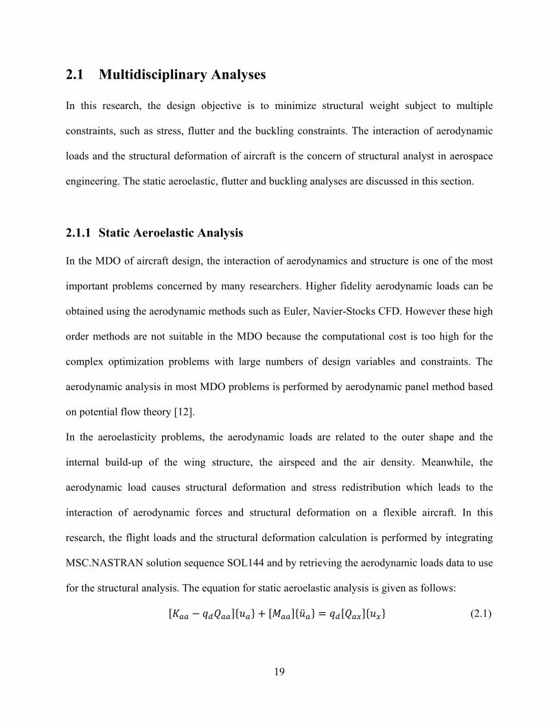
2.1  Multidisciplinary Analyses ............................................................................................ 19 

2.1.1  Static Aeroelastic Analysis ..................................................................................... 19 

2.1.2  Modal Analysis ....................................................................................................... 22 

2.1.3  Flutter Analysis ....................................................................................................... 22 

2.1.4  Buckling Analysis ................................................................................................... 25 

2.2  Geometry Parameterization ............................................................................................ 26 

2.2.1  Geometry Parameterization of Curvilinear SpaRibs ............................................... 26 

2.2.2  Geometry Parameterization of Curvilinear Stiffeners ............................................ 29 

2.3  Global-Local Optimization Framework ......................................................................... 30 

2.3.1  Global Wing Optimization ...................................................................................... 30 

2.3.2  Local Panel Optimization ....................................................................................... 32 

2.3.3  Integration of Global Wing and Local Panel Optimization .................................... 34 

2.4  Summary ........................................................................................................................ 35 

Chapter 3 Global Wing Optimization: EBF3WingOpt ............................................................ 36 

3.1  Optimization of Boeing N+2 HSCT Wing ..................................................................... 37 

3.1.1  Boeing N+2 HSCT Wing Description .................................................................... 37 

3.1.2  Optimization Procedure of Boeing N+2 HSCT Wing ............................................ 39 

3.1.3  Baseline Boeing N+2 HSCT Configuration ........................................................... 45 

3.1.4  Optimization Results of Boeing N+2 HSCT Aircraft ............................................. 46 

3.2  Optimization of NASA Common Research Model ........................................................ 54 

ix

3.2.1  NASA Common Research Model (CRM) Wing Description ................................. 54 

3.2.2  Design Variables in Optimization of Subsonic CRM Wing ................................... 55 

3.2.3  Optimization Procedure of NASA CRM Wing ...................................................... 58 

3.2.4  Optimization Results of Common Research Model ............................................... 60 

3.2.5  Pre-stressed Modes and Unstressed Modes in Flutter Analysis ............................. 64 

3.3  Summary ........................................................................................................................ 65 

Chapter 4 EBF3PanelOpt: Un-Stiffened Panel Optimization .................................................. 67 

4.1  Local Panel Optimization Procedure of CRM Wing ..................................................... 68 

4.2  Buckling Analysis of Local Panel .................................................................................. 72 

4.3  Panel Thickness Optimization ........................................................................................ 74 

4.4  Results of Un-Stiffened Panel Optimization .................................................................. 77 

4.5  Summary ........................................................................................................................ 82 

Chapter 5 EBF3PanelOpt: Stiffened Panel Optimization ....................................................... 83 

5.1  Description of Stiffened Panel ....................................................................................... 84 

5.2  Interconnection between Global Wing and Stiffened Panel .......................................... 85 

5.3  Panel Thickness Optimization of Stiffened Panel .......................................................... 88 

5.4  Effect of Stiffener Size in the Stiffened Panel Optimization ......................................... 91 

5.5  Number of Stiffeners ...................................................................................................... 92 

5.6  Stiffened Panel Optimization Procedure ........................................................................ 95 

5.7  Results of Stiffened Panel Optimization of CRM Wing ................................................ 97 

x

5.8  Integration of Global Wing and Local Panel Optimization ......................................... 102 

5.8.1  Global-Local Optimization Framework ................................................................ 102 

5.8.2  Approximate Stiffened Panel Optimization .......................................................... 105 

5.8.3  Initial Panel Thickness .......................................................................................... 109 

5.8.4  Results of Integrated Global-Local Optimization ................................................. 110 

5.9  Optimization of Panel with Curvilinear Stiffeners ....................................................... 114 

5.10  Summary ...................................................................................................................... 122 

Chapter 6 ..................................................................................................................................... 123 

Future Research .......................................................................................................................... 123 

Bibliography ............................................................................................................................... 125 

xi

List of Figures

Figure 1.1:  Buckling Analysis of Flat Plate .............................................................................. 12 

Figure 1.2:  Stiffened Panel ........................................................................................................ 13 

Figure 2.1: Flutter Velocity of Jet Transport Wing……………………………………………..24

Figure 2.2: Linked Shape Parameterization. (Locatelli et al. [80]) ............................................. 27 

Figure 2.3: Example of NASA CRM Wing with Curvilinear SpaRibs ....................................... 28 

Figure 2.4: Parameterization of Curvilinear Stiffeners. ............................................................... 29 

Figure 2.5: Global-Local Optimization Framework .................................................................... 31 

Figure 2.6: Flow Diagram of Local Panel Analysis. ................................................................... 33 

Figure 3.1: Boeing N+2 HSCT Aircraft Concept……………………………………………….38 

Figure 3.2: Boeing N+2 HSCT Aircraft Structural Configuration. (Chen et al. 2010 [83]) ...... 38 

Figure 3.3: Flight Envelop of Boeing HSCT Aircraft Concept. (Chen et al. 2010 [83]) ............ 39 

Figure 3.4: Example of Internal Wing Structure Configuration Generated with EBF3WingOpt 40 

Figure 3.5: Aerodynamic Elements of Boeing HSCT Wing ....................................................... 42 

Figure 3.6: Spline Nodes in Boeing HSCT Wing ........................................................................ 43 

Figure 3.7: Global Optimization Framework for Boeing N+2 HSCT Wing ............................... 44 

Figure 3.8: Finite Element Mesh of the Portion of the Re-designed Structure ............................ 46 

Figure 3.9: Optimum Topology Computed at the First Optimization Step. ................................ 48 

xii

Figure 3.10: Thickness Distribution of the Optimized Structure (in). ......................................... 49 

Figure 3.11: von Mises Stress Distribution Associated to the 2.5 g Pull-Up Maneuver ............. 50 

Figure 3.12: von Mises Stress of the Aircraft Structure .............................................................. 52 

Figure 3.13: Flutter Analysis Results........................................................................................... 53 

Figure 3.14: Example of NASA Common Research Model ........................................................ 54 

Figure 3.15: Aerodynamic Elements of NASA CRM Wing ....................................................... 55 

Figure 3.16: Example of Spline Nodes in NASA CRM Wing .................................................... 55 

Figure 3.17: Nonlinear Thickness Fields ..................................................................................... 58 

Figure 3.18: Optimized Thickness Fields .................................................................................... 61 

Figure 3.19: von Mises Stress Distribution.................................................................................. 62 

Figure 3.20: Optimal Design Using Nonlinear Thickness Fields ................................................ 63 

Figure 3.21: Global Modes of Optimal CRM Wing .................................................................... 63 

Figure 3.22: Flutter Dynamic Pressure ........................................................................................ 64 

Figure 3.23: Flutter Frequency .................................................................................................... 65 

Figure 4.1: CRM Design with 37 Straight Ribs Provided by NASA…………………………...68

Figure 4.2: Results of Baseline CRM Design with 37 Straight Ribs ........................................... 69 

Figure 4.3: Local Panel Optimization Procedure ......................................................................... 70 

Figure 4.4: Modification of Local Panel Thickness ..................................................................... 71 

Figure 4.5: Boundary Conditions in Local Panel Analysis.......................................................... 73 

Figure 4.6: 1st Buckling Mode Shape of Local Panel with Various Boundary Conditions ......... 73 

Figure 4.7: Comparison of Move Limit 1 and 2 of Panel Thickness ........................................... 76 

Figure 4.8: Comparison of Move Limit 2 and 3 of Panel Thickness ........................................... 76 

Figure 4.9: Convergence History of Un-Stiffened Panel Optimization of NASA CRM Wing ... 78 

xiii

Figure 4.10: Fundamental Buckling Eigenvalues of Optimal Local Panels ................................ 78 

Figure 4.11: Buckling Mode Shapes of Un-Stiffened Panel Optimization Design ..................... 80 

Figure 4.12: Optimal Thicknesses of Wing Panels ...................................................................... 81 

Figure 4.13: von Mises Stress of Un-Stiffened Panel Optimization Design ............................... 81 

Figure 4.14: Displacement in Z Direction of Un-Stiffened Panel Optimization Design ............. 82 

Figure 5.1: CRM Wing with Stiffened Panels…………………………………………………..84

Figure 5.2: Boundary Condition of Stiffened Panel .................................................................... 85 

Figure 5.3: Interpolation of Displacements ................................................................................. 86 

Figure 5.4: Comparison of Stress Distribution ............................................................................ 87 

Figure 5.5: Fundamental Buckling Mode Shapes of Stiffened Panel .......................................... 89 

Figure 5.6: Fundamental Buckling Eigenvalues of Stiffened Panel ............................................ 90 

Figure 5.7: Process of Stiffened Panel Thickness Optimization .................................................. 91 

Figure 5.8: Buckling Mode Shapes of Stiffened Panels with Different Stiffener Height ............ 92 

Figure 5.9: Stiffened Panel with 10 Stiffeners ............................................................................. 93 

Figure 5.10: Number of Stiffeners in the Stiffened Panels .......................................................... 94 

Figure 5.11: Optimization Process of Stiffener Size ................................................................... 96 

Figure 5.12: Thickness Distribution of Un-Stiffened and Stiffened NASA CRM Wing ............ 98 

Figure 5.13: Optimal Thickness of Spars and Ribs of Stiffened NASA CRM Wing .................. 99 

Figure 5.14: Convergence History of Stiffened Panel Optimization of NASA CRM Wing ....... 99 

Figure 5.15: Fundamental Buckling Eigenvalues of Optimal Local Panels .............................. 100 

Figure 5.16: von Mises Stress of Stiffened Panel Optimization Design.................................... 100 

Figure 5.17: Displacement in Z Direction of Stiffened Panel Optimization Design ................. 101 

Figure 5.18: Fundamental Buckling Mode Shapes of CRM Design with 37 Ribs .................... 101 

xiv

Figure 5.19: Optimal Weight Calculation of Stiffened CRM Wing .......................................... 103 

Figure 5.20: Integrated Global-Local Optimization Framework ............................................... 104 

Figure 5.21: Upper Skin Panels ................................................................................................. 106 

Figure 5.22: Comparison of Optimal Thickness of Upper Skin Panels ..................................... 107 

Figure 5.23: Decomposition of CRM Wing Panels ................................................................... 107 

Figure 5.24: Cumulative Probability Distribution of Weight Error ........................................... 109 

Figure 5.25: Initial Panel Thickness Calculation of Stiffened Panel Design ............................. 110 

Figure 5.26: Convergence History of Optimal Wing Weight .................................................... 111 

Figure 5.27: Approximate Optimal Weight of CRM Wing with Stiffened Panels .................... 112 

Figure 5.28: Geometry of CRM Wing with 9 Inner Wing Ribs and 17 Outer Wing Ribs ........ 112 

Figure 5.29: Thickness Distribution of Optimal CRM Design .................................................. 112 

Figure 5.30: Typical Load Cases of Panels ............................................................................... 114 

Figure 5.31: Geometry Parameterization of Curvilinear Stiffeners ........................................... 115 

Figure 5.32: Optimization Procedure of Curvilinear Stiffeners ................................................. 116 

Figure 5.33: History of Curvilinear Stiffeners Optimization Using PSO .................................. 117 

Figure 5.34: Curvilinear Stiffener Optimization Using Two-Step Approach ............................ 117 

Figure 5.35: Stress Resultant of an Example Stiffened Panel ................................................... 118 

Figure 5.36: Stiffener Optimization Using Y-Component Stress .............................................. 119 

Figure 5.37: Average Y-Component Stress in Panel Sections .................................................. 120 

Figure 5.38: Fundamental Buckling Mode Shape of Stiffened Panel ....................................... 121 

xv

List of Tables

Table 2.1: Parameters Description in Linked Shape Method. (Locatelli et al. [80]) ................. 28 

Table 2.2: Parameters of Curvilinear Stiffeners .......................................................................... 29 

Table 3.1: Weight Summary for Boeing N+2 Aircraft Concept (Chen et al. 2010 [83])……….45

Table 3.2: Mass Summary for Boeing N+2 Aircraft Concept Optimized with SpaRibs. ............ 46 

Table 3.3: Kreisselmeier-Steinhauser Coefficients for Different Flight Conditions ................... 47 

Table 3.4: Flutter Constraint Coefficients of Optimal Configuration. ......................................... 47 

Table 3.5: Optimized Structure Performance Compared. ............................................................ 53 

Table 3.6: Shape Design Variables .............................................................................................. 56 

Table 3.7: Boundary of Shape Design Variables of Spars and Ribs ........................................... 56 

Table 3.8: Aluminum Alloy 2024-T3 Mechanical Properties ..................................................... 57 

Table 3.9: Size Design Variables ................................................................................................. 58 

Table 3.10: Comparison of Optimal Designs using Different Thickness Fields ......................... 61 

Table 3.11: Constraints of Global Optimal Design with Nonlinear Thickness Fields ................ 62 

Table 4.1: Fundamental Buckling Eigenvalues of Local Panel…………………………………73

Table 4.2: Results of Un-Stiffened Panel Optimization .............................................................. 77 

Table 4.3: Buckling Eigenvalues of the First Ten Modes ........................................................... 80 

Table 5.1: Effect of Number of Stiffeners in the Stiffened Panel Optimization………………...93

Table 5.2: Results of Local Panel Optimization .......................................................................... 98 

xvi

Table 5.3: Error of Approximate Stiffened Panel Optimization of Panel Groups ..................... 108 

Table 5.4: Comparison of Computation Time ........................................................................... 108 

Table 5.5: Constraints of Optimal CRM Design ....................................................................... 113 

Table 5.6: Design Variables in Curvilinear Stiffener Optimization .......................................... 115 

Table 5.7: Optimization Results of Curvilinear Stiffened Panel ............................................... 118 

Table 5.8: Comparison of Stiffener Optimization Schemes ...................................................... 121 

xvii

Nomenclature

MDO Multidisciplinary Design Optimization

PSO Particle Swarm Optimization

GBO Gradient Based Optimization

GA Genetic Algorithm

cr Critical Buckling Stress

x Design Variables

KS() Kreisselmeier-Steinhauser Stress Coefficient

Kreisselmeier-Steinhauser Parameter

y Yield Stress

vmi ith Finite Element von Mises Stress

Ai ith Finite Element Area

BF Buckling Factor

SF Safety Factor

uz Vertical Displacement

topt Local Panel Optimized Thickness

λp Fundamental Buckling Eigenvalue

OML Outer Mold Line

Qcr Critical Flutter Dynamic Pressure

xviii

Qfl Flight Condition Dynamic Pressure

Fsubsonic Subsonic Flutter Constraint Coefficient

Fsupersonic Supersonic Flutter Constraint Coefficient

tskin Skin Panel Thickness

bskin Spacing between Two Adjacent Stiffeners

DV Design Variables

1

Chapter 1

Introduction

1.1 Background

Multidisciplinary Design Optimization (MDO) has been used in a number of fields, particularly

in the aircraft design process. Because of the emergence of innovative aircraft design concepts,

the aircraft design process using the empirical structural and aerodynamic equations based on

databases obtained from past experience may not be reliable or efficient for a non-conventional

aircraft structure design. The aircraft design needs to consider different disciplines, such as the

aerodynamics, structural analysis, propulsion, control and dynamics, and the manufacturing and

operating costs. The design of aircraft wing structure consists of the internal structural layout, the

size of the structural components, the aerodynamic loads and the aeroelastic response of the

structure. In particular, the study of the interaction between the structure and the aerodynamics is

critical for designing transport aircraft and must be considered in an optimization framework that

aims to devise more efficient wing structures.

2

In the multidisciplinary design, there are many conflicting objectives that need to be considered.

Reducing the weight is often one of the most important objectives in aircraft structural

optimization, while various additional constraints should be imposed on the aircraft. Therefore,

design engineers need to take into account multidisciplinary constraints using appropriate fidelity

during the conceptual and preliminary design stages and they need optimization tools to

accomplish this complex task.

A MDO problem is usually decomposed into multiple sub-systems so as to reduce the

complexity and computational cost of the optimization process. In the optimization problem of

an aircraft wing with local panels bordered by spars and ribs, the design variables can be divided

into two groups: global wing design variables which define the topology of wing internal

structure; local panel design variables which define the details of local panel models, like the

panel thickness and stiffeners. Therefore, the wing variables and local panel variables can be

optimized in global wing optimization and local panel optimization, respectively. Based on this

idea, a global-local optimization framework is developed for the transport aircraft wing design to

integrate the wing and panel optimization.

One of the most important challenges of the global-local optimization is the high computational

cost due to multidisciplinary analyses of the complex wing structure. In the previous research

about the global-local optimization of aircraft wing, the local panels are usually modeled as un-

stiffened panels, or using surrogate models to substitute the stiffened panels to save

computational cost. This research represents the first time a global-local optimization framework

is implemented with medium fidelity tools for the aircraft wing with stiffened panels.

Another important aspect of this research is the application of the new concept of curvilinear

stiffening members to improve the efficiency of the structure load bearing mechanism and to

3

enlarge the design space. In this research, the use of curvilinear spars and ribs (SpaRibs), and

stiffened panel with curvilinear stiffeners have been integrated in the global-local optimization

framework.

In the MDO study, a general optimization tool needs to be developed, not only designed for a

particular aircraft wing, but also can be applied for other wing designs. Therefore, the geometry

parameterization of the wing structure is very important for the MDO research.

This dissertation is structured as follows: firstly, the literature review about previous work which

is closely related to this research is presented. The details about multidisciplinary analyses,

geometry parameterization of wing stiffening members, and the global-local multidisciplinary

optimization framework are described in Chapter 2. In Chapter 3, the global wing optimization

has been applied to two aircraft wing structures: the Boeing high speed commercial transport

aircraft concept (Boeing HSCT) and a public-domain NASA wing structure, commonly referred

to as the Common Research Model (CRM Wing). Chapter 4 discusses the local panel

optimization and presents the application on the NASA CRM wing with un-stiffened panels. The

stiffened panel optimization and the application of integrated global-local optimization are

discussed in Chapter 5. Finally, Chapter 6 concludes the current research and discusses the future

work.

4

1.2 Literature Review

1.2.1 Multidisciplinary Design Optimization

The aim of a multidisciplinary design optimization (MDO) study is to find an efficient approach

to incorporate all relevant disciplines and analytical tools simultaneously in a single optimization

problem.

The study of MDO originates in structural optimization, which can be traced back to Schmit’s

innovative paper published in 1960 [1]. In his work [1-3], the numerical optimization technique

was coupled with finite element analysis, in order to search the optimum design in an efficient

way. Motivated by the success of structural optimization, the MDO approach has been widely

applied in the aircraft structural design since the 1970s thanks to the improvement of the

computer technology. Haftka [4-6], Sobieszczanski-Sobieski [7] and their collaborators studied

the optimization of aircraft wing including the interaction of multiple disciplines, such as

strength, aeroelasticity, and buckling.

In the mathematical view, MDO problem is a constrained nonlinear programming problem to

maximize or minimize a particular objective function, subject to the constraints for multiple

disciplines. According to the number of objectives, the aircraft design optimization problem can

be classified into single objective problems and multi-objective problems. For the single

objective problem, the most common objective, in structural optimization, is minimizing the

structural weight. Multi-objective optimization which involves two or more objectives can be

solved by calculating a set of Pareto optimal solutions [8-10]. In the multidisciplinary

optimization, penalty method is widely used to describe the values of multiple constraints [11].

One of the major challenges in MDO study is how to manage the coupling of the multiple

disciplines in the constraints. In most MDO problems, the discipline analyses are mutually

5

interdependent. The results of one analysis may depend on the output of other analyses. The

interdisciplinary coupling in the MDO increases the complexity of the problem. A large number

of design variables are required for all disciplines in the MDO, which cause more computational

and organizational challenges. Because of the interaction of different disciplines, MDOs

typically cost much more than the sum of costs of the sequential single discipline optimizations

[12]. For the complex MDO problem, it is a very important to find a proper procedure to

organize the optimization and reduce the computational cost. Rabeau [13] classified the MDO

methodologies into hierarchical decomposition or non-hierarchical decomposition:

(1) Hierarchical decomposition: complex optimization problem is decomposed into multilevel

sub-systems. For instance, the aircraft structure is divided into wingbox, fuselage, control

surfaces, tail and engine in the first level. Then in the second level, the wingbox can be divided

into top skin, bottom skin, spars and ribs. The wing skins can be decomposed into a number of

panels in the third level. A complex system can be optimized using a combination of basic sub-

systems through the multilevel decomposition.

(2) Non-hierarchical decomposition: all the sub-systems are in the same level, in other words

there is no reason to optimize one sub-system before another.

In a recent review, Martines [14] classified all the MDO procedures into two types: monolithic

architecture and distributed architecture. The monolithic architecture means that the researchers

solved the MDO problem as a single optimization problem. Distributed architectures can be

implemented by decomposing the structure or design variables into multiple sub-systems, then

optimizing the sub-systems subject to local constraints.

In the monolithic architectures, a widely used MDO procedure is the All-at-Once optimization

[12, 14], which means the optimization is considered as an integrated system, all design variables

6

and all constraints of various disciplines are included in one single optimization process. The

All-At-Once optimization procedure is easier to understand and implement. However, for the

problems with complex mathematical model and interaction between multiple disciplines, this

method may be inefficient because it requires too many design variables and constraints to

describe the whole problem. For the optimization problems with a large number of design

variables or constraints, the optimization process can be improved using a sequential multiple-

step optimization approach [15, 16]. Only a part of design variables or constraints are included in

each step of the optimization process. Locatelli et al. [15] implemented a two-step optimization

for a supersonic wing structure, in which all the design variables are classified as shape design

variables or size design variables. The first step optimization focuses on optimizing the shape

design variables. The second step optimization is based on the results of the first step

optimization, to refine the size design variables.

In the distributed MDO architectures, the complex optimization problem of engineering system

is decomposed into multiple smaller tasks to improve the overall optimization efficiency.

Numerous decomposition strategies have been proposed to reduce the complexity and

computational cost of MDO. Kroo and his collaborators studied collaborative optimization [24,

25]. Collaborative optimization is designed to allow each discipline to solve its sub-system

problem in parallel with the others. Sobieszczanski-Sobieski et al. [17, 18] divided the

optimization problem into two sub-levels: system level and subsystem level. The design

variables of the entire structure are optimized in the system level optimization. The subsystem

design variables and constraints are evaluated in the subsystem level optimization. The smaller

subsystems can be executed simultaneously and are compatible with parallel computing using

multiprocessors. For some MDO problems with a complex structure, the global structure is

7

usually decomposed into smaller local structures. This kind of decomposition scheme is also

named as global/local design optimization. Some authors have applied the global/local design

optimization in the aircraft wing design [19-21]. Ciampa and Nagel [20] studied the global/local

optimization for a cantilever wing. In their research, a global level optimization which includes

both shape and size design variables of the wing structure was performed. Then the global

optimal design was decomposed into many local panels. The thicknesses of local panels were

refined in local panel optimization by optimizing the stiffened local panels to minimize the

structural mass. Considering that the optimal results of local optimization need to be fed back to

the global model for updating the properties of local models, the global wing optimization and

local panel optimization need to be integrated into an iterative global-local optimization

framework [20, 21].

The interaction between sub-systems increases the complexity of MDO problems. If the design

variables of one sub-system are not independent to the design variables of other sub-systems, or

the output responses of one sub-system are needed for several other sub-systems as input

variables, the optimization problem will become more difficult to solve. The quasi-separable

decomposition, as discussed by Haftka et al. [22], means the subsystem consists of local design

variables and global system variables, but no variables from other subsystems. The idea of

solving this kind of problem is to give each subsystem a local model, and then ask each

subsystem to independently search the optimum in the constraint margins. Gürdal et al. [23]

studied the multidisciplinary design optimization of a composite wing considering strength,

buckling, aerodynamic twist and aileron effectiveness constraints. In their finite element model,

each wing panel bordered by the stringers and ribs was represented using one element. The

8

thicknesses of the wing panels were independent in the global-local optimization therefore they

can be optimized simultaneously.

1.2.2 Optimization Algorithm

Optimization methods play a major role in solving the MDO problems by searching through the

design space to minimize or maximize the objection function. For the complex optimization

problem with a large number of design variables, a considerably high-dimensional design space

is required, which creates an exponential challenge for optimization.

The optimization algorithms essentially can be classified into two groups: gradient-based

methods and non-gradient-based methods. The origins of gradient methods are nearly as old

as calculus, dating back to Isaac Newton, Leonhard Euler, Daniel Bernoulli, and Joseph Louis

Lagrange. The gradient-based methods determine the optimal design using the gradient

information from a first-order design sensitivity analysis. The recursive formulas of gradient-

based methods are derived based on the Karush–Kuhn–Tucker (KKT) necessary conditions for

an optimal design [26]. Sequential quadratic programming (SQP) was developed for nonlinear

gradient optimization. SQP methods are used for the problems where the objective function and

the constraints are twice continuously differentiable. Approximation concepts were constructed

by Fleury and Schmit [27]. In combination with other techniques, such as constraint deletion,

reciprocal approximation and design variable linking, they have been successfully applied in

structural optimization. Canfield [28] developed a Rayleigh Quotient approximation to improve

the accuracy of eigenvalue approximations. The gradient-based methods normally find the

optimal point close to the starting design point, in other words it is possible to get a local

optimum but not the global optimum.

9

The non-gradient methods do not need gradient information at the design points. These methods

include nature-inspired evolutionary methods and the related swarm algorithm, such as, genetic

algorithm (GA) [29], particle swarm optimization (PSO) [30, 31], that have recently

demonstrated their success as well as popularity in MDO applications. Both the GA [32] and

PSO [33] methods have been extensively applied in transport aircraft wing optimization. Those

methods are successful applications with the philosophy of bounded rationality and decentralized

decision making for exploiting the optimal design in the global design space.

The Genetic Algorithms (GA) have become one of the most employed solution methods in

engineering problems since they can handle integer, binary, discrete and continuous variables

and is effective with nonlinear functions and non-convex design spaces. The method is based on

Darwin’s theory of natural adaptation and biological evolution, which is translated into

algorithmic terms through the computational operators of selection, crossover and mutation.

Marin et al. [34] developed a two-step optimization framework using neural networks and

genetic algorithms for a composite stiffened panel, showing a reduction of the computational

cost of about 90% with suitable accuracy. Zingg et al. [35] compared the efficiency of genetic

algorithm and gradient based methods in aerodynamic shape optimization. In their conclusion,

the genetic algorithm is more suited to preliminary design where low-fidelity models are used.

However, the gradient based methods are more appropriate for detailed design where high-

fidelity models and tight convergence tolerances are needed.

A number of advantages with respect to other evolutionary algorithms are attributed to PSO

making it a prospective candidate for optimum structural design. The PSO-based algorithm is

robust and well suited to handle nonlinear, non-convex design spaces with discontinuities,

exhibiting fast convergence characteristics. Nevertheless, those algorithms cannot fully satisfy

10

the MDO problem need for the complex and computationally expensive problems so that some

minor/major modifications are demanded depending on the nature of difficulty. Hybrid

algorithms can integrate the advantages of the PSO and gradient methods. Plevris et al. [36]

present an enhanced PSO algorithm combined with a gradient-based sequential quadratic

programming (SQP) method for solving structural optimization problems. The modified PSO

incorporates the exploiting the whole design space and searching the neighborhood of the global

optimum. Then the mathematical optimizer, starting from the best estimate of the PSO and using

gradient information, accelerates convergence toward the global optimum. Hajikolaeil et al. [37]

introduced a self-accelerated PSO method to improve the velocity updating process. The idea is

to build a metamodel from all previous particles from the beginning of the optimization process

until the current step. Then, the algorithm updates new velocities using the parameters obtained

from the metamodel.

A focus of current research on optimization methods is to improve the quality of approximations

and reduce the number of iterations and thus the total optimization time and cost. Surrogate

models are widely used in the computationally expensive optimizations, such as response

surfaces optimization [38], neural networks method, and kriging [39]. It uses computationally

cheap hierarchical surrogate models to replace the exact computationally expensive objective

functions to reduce the computational cost.

Tradeoff between accuracy and computational cost is an important topic in the study of MDO.

Approximation technique that helps to eliminate the computational challenge has been

extensively studied, especially for the engineering problems with complex structures. For most

complex problems, design variables and response quantities are used to improve the accuracy of

the approximate optimization. Response surface method (RSM) was introduced by Box and

11

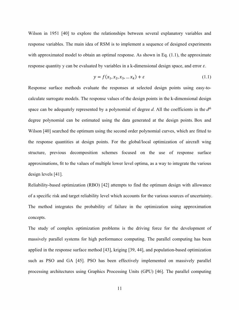
Wilson in 1951 [40] to explore the relationships between several explanatory variables and

response variables. The main idea of RSM is to implement a sequence of designed experiments

with approximated model to obtain an optimal response. As shown in Eq. (1.1), the approximate

response quantity y can be evaluated by variables in a k-dimensional design space, and error .

, , , … (1.1)

Response surface methods evaluate the responses at selected design points using easy-to-

calculate surrogate models. The response values of the design points in the k-dimensional design

space can be adequately represented by a polynomial of degree d. All the coefficients in the dth

degree polynomial can be estimated using the data generated at the design points. Box and

Wilson [40] searched the optimum using the second order polynomial curves, which are fitted to

the response quantities at design points. For the global/local optimization of aircraft wing

structure, previous decomposition schemes focused on the use of response surface

approximations, fit to the values of multiple lower level optima, as a way to integrate the various

design levels [41].

Reliability-based optimization (RBO) [42] attempts to find the optimum design with allowance

of a specific risk and target reliability level which accounts for the various sources of uncertainty.

The method integrates the probability of failure in the optimization using approximation

concepts.

The study of complex optimization problems is the driving force for the development of

massively parallel systems for high performance computing. The parallel computing has been

applied in the response surface method [43], kriging [39, 44], and population-based optimization

such as PSO and GA [45]. PSO has been effectively implemented on massively parallel

processing architectures using Graphics Processing Units (GPU) [46]. The parallel computing

12

toolbox has been integrated in commercial software such as MATLAB, and optimization

software such as VisualDOC and DAKOTA, which can be easily implemented by the users.

1.2.3 Instability of Local Panel

The structural instability of wing skins, which consist of smaller local panels bordered by spars

and ribs, is a crucial concern in aircraft structural design. The panel may buckle in a variety of

modes depending upon its loading, boundary conditions and panel sizes. Lundquist and Stowell

[47] studied the buckling of a flat rectangular plate supported along all edges. The critical

buckling stress of that plate with compressive loads applied on two opposite edges can be given

as following formula

(1.2)

where k is a constant depends upon the particular shape of the panel being investigated. is

the panel thickness, and is the length of the panel edge that is perpendicular to the

compressive loads.

Figure 1.1: Buckling Analysis of Flat Plate

13

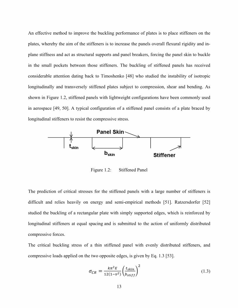
An effective method to improve the buckling performance of plates is to place stiffeners on the

plates, whereby the aim of the stiffeners is to increase the panels overall flexural rigidity and in-

plane stiffness and act as structural supports and panel breakers, forcing the panel skin to buckle

in the small pockets between those stiffeners. The buckling of stiffened panels has received

considerable attention dating back to Timoshenko [48] who studied the instability of isotropic

longitudinally and transversely stiffened plates subject to compression, shear and bending. As

shown in Figure 1.2, stiffened panels with lightweight configurations have been commonly used

in aerospace [49, 50]. A typical configuration of a stiffened panel consists of a plate braced by

longitudinal stiffeners to resist the compressive stress.

Figure 1.2: Stiffened Panel

The prediction of critical stresses for the stiffened panels with a large number of stiffeners is

difficult and relies heavily on energy and semi-empirical methods [51]. Ratzersdorfer [52]

studied the buckling of a rectangular plate with simply supported edges, which is reinforced by

longitudinal stiffeners at equal spacing and is submitted to the action of uniformly distributed

compressive forces.

The critical buckling stress of a thin stiffened panel with evenly distributed stiffeners, and

compressive loads applied on the two opposite edges, is given by Eq. 1.3 [53].

(1.3)

14

where k is a constant depends upon the particular shape of the panel being investigated. is

the panel thickness, and is the spacing between two adjacent stiffeners. This analytic

solution shows the critical buckling stress is related to the ratio of plate thickness and spacing

between stiffeners.

The design optimization of stiffened panel has been exhaustively studied to identify the lightest-

weight stiffening configuration subject to stress and buckling constraints. Design variables can

be the stiffener spacing, stiffener height and thickness, skin thickness, and stiffening

configuration.

The panel stiffened by blade stiffeners was studied by many researchers [54, 55, 56]. Herencia et

al. studied the optimization of composite panel with T-shape stiffeners [57]. Vitali optimized the

stiffener spacing, panel thickness, and thickness of stiffener components of hat stiffeners.

The most common design of stiffened panels is that the panel is stiffened by longitudinal

stiffeners [58, 59, 60, 61]. Jaunky et al. studied the buckling of grid-stiffened composite panel

with both axial and transverse stiffeners [62].

A number of optimization methods have been applied in the optimization of stiffened panel.

Gradient based method and particle swarm method are compared in the stiffened panel

optimization [63]. Parallel computing is implemented with genetic algorithm [59, 62, 63] or

response surface method [60, 64].

In the finite element analysis, as compared to the un-stiffened panels, much smaller size of

elements are required for meshing the panel with a large number of stiffeners. In order to avoid

the high computational cost, buckling analysis can be approached with two methods: smearing

the properties of the stiffener elements over the skin or treating the stiffeners as beam elements

with an effective flexural rigidity. Walch et al. [65] developed a tool S4WING to efficiently

15

predict stiffness, spanwise and chordwise mass distribution in a wingbox at conceptual design

stages. It uses a physics-based simplification process for a finite element wing box model in

which the stiffeners are smeared in the skin to reduce the number of elements of the model.

1.2.4 Curved Stiffening Members

Classic structural design for aircraft wingbox uses simple components such as straight spars and

ribs, quadrilateral wing skin panels with straight stiffeners. The components are connected using

bolts and rivets or by welding. A new design philosophy, using curvilinear spars and ribs

(SpaRibs), pioneered by Kapania and his group at VT (Locatelli, Mulani and Kapania [66, 67]),

has been introduced based on emerging manufacturing technologies such as Friction Stir

Welding(FSW) [68, 69] and Electron Beam Free Form Fabrication (EBF3) [70]. In these

innovative technologies, the structure is manufactured as an integrated part instead of using

mechanically fastened structural components. Based on the new technology, the concept of

curvilinear stiffening members with non-uniform thickness have been implemented in design of

wing internal structure ([66, 67, 71]). Compared with the conventional straight spars, ribs and

stringers, the advantage of curved stiffening members resides in the coupling between bending

and torsional rigidity. That means bending and torsional deformation can be reduced by suitably

placing curvilinear SpaRibs and stiffeners. The concept of curvilinear stiffening members

enlarges the design space and provides possibility for a more efficient aircraft design.

Multidisciplinary optimization of stiffened panel with curvilinear stiffeners is studied [66, 72, 73,

74] with an objective of minimizing the mass of panels and subject to constraints on buckling,

von Mises stress, and crippling or local failure of the stiffener.

16

1.3 Research Objectives

The aim of this research is to develop a multidisciplinary design optimization framework for

transport aircraft wing design. Static aeroelastic, flutter and buckling analyses are integrated in

the optimization framework, all in an effort to reduce structural weight, when subjected to stress,

displacement, flutter and buckling constraints for multiple flight conditions. The optimization

framework is integrated by wing optimization EBF3WingOpt and panel optimization

EBF3PanelOpt.

In the EBF3WingOpt, a new design concept curvilinear spars and ribs (SpaRibs) has been

introduced to take advantage of the structural deformation couplings provided by the curvature

and to design more efficient and lighter structures. The use of curvilinear internal structures

allows for an enlarged design space which gives the designers more flexibility to tailor the

structure according to the stress distribution. In this research, geometry parameterization of

SpaRibs, aeroelasticity analysis and topology/sizing optimization have been integrated into

global wing optimization framework EBF3WingOpt.

The wing skins are divided into local panels by the SpaRibs. A framework EBF3PanelOpt is

developed for the optimization of un-stiffened or stiffened panels considering buckling and stress

constraints. In this research, a global-local multidisciplinary design optimization procedure has

been developed to incorporate EBF3WingOpt and EBF3PanelOpt for the optimization of

aircraft wing. The commercial software MSC.NASTRAN, which incorporates the static,

buckling and aeroelasticity module, is selected as finite element analysis tool. The optimization

framework is developed using Python and MATLAB programming to integrate the geometry and

mesh generation, finite element analysis and optimization algorithms.

The objectives of this research can be summarized as:

17

Developing a multidisciplinary design framework for the optimization of aircraft wing

structure which includes the use of curvilinear stiffening members (SpaRibs).

Developing an efficient global wing optimization framework to optimize the size and

topology of the wing internal structure.

Developing a local panel optimization framework for optimizing the un-stiffened or

stiffened panels.

Implementing the integration of global-local multidisciplinary optimization framework

using commercially available analysis software as MSC. PATRAN, MSC. NASTRAN.

18

Chapter 2

Global-Local Optimization Framework

The global-local MDO framework EBF3GLWingOpt, which integrates the global wing

optimization module EBF3WingOpt and local panel optimization module EBF3PanelOpt, is

discussed in this chapter. The integration of multidisciplinary analyses, such as static aeroelastic,

flutter, and buckling analyses, is introduced in the first section. The second section presents the

geometry parameterization of wing structure that consists of curvilinear spars, ribs or stiffeners.

Then the optimization procedure of global wing optimization and local panel optimization is

described.

19

2.1 Multidisciplinary Analyses

In this research, the design objective is to minimize structural weight subject to multiple

constraints, such as stress, flutter and the buckling constraints. The interaction of aerodynamic

loads and the structural deformation of aircraft is the concern of structural analyst in aerospace

engineering. The static aeroelastic, flutter and buckling analyses are discussed in this section.

2.1.1 Static Aeroelastic Analysis

In the MDO of aircraft design, the interaction of aerodynamics and structure is one of the most

important problems concerned by many researchers. Higher fidelity aerodynamic loads can be

obtained using the aerodynamic methods such as Euler, Navier-Stocks CFD. However these high

order methods are not suitable in the MDO because the computational cost is too high for the

complex optimization problems with large numbers of design variables and constraints. The

aerodynamic analysis in most MDO problems is performed by aerodynamic panel method based

on potential flow theory [12].

In the aeroelasticity problems, the aerodynamic loads are related to the outer shape and the

internal build-up of the wing structure, the airspeed and the air density. Meanwhile, the

aerodynamic load causes structural deformation and stress redistribution which leads to the

interaction of aerodynamic forces and structural deformation on a flexible aircraft. In this

research, the flight loads and the structural deformation calculation is performed by integrating

MSC.NASTRAN solution sequence SOL144 and by retrieving the aerodynamic loads data to use

for the structural analysis. The equation for static aeroelastic analysis is given as follows:

(2.1)

20

where and are structural stiffness matrix and structural mass matrix, respectively. is

the vector of structural displacements. is the vector of displacements of aerodynamic extra

points, such as aerodynamic control surface deflections and rigid body motions. is dynamic

pressure. is aerodynamic influence coefficient matrix, which is used to calculate the

aerodynamic forces due to structural deformation. is the aerodynamic matrix due to the

deflections of aerodynamic extra points.

MSC.NASTRAN provides the Doublet Lattice Method (DLM) [75, 76] and ZONA51 [77]

method for the computation of the aerodynamic loads at subsonic and supersonic regimes,

respectively. Both methods are based on the linearized aerodynamic potential theory, which

neglects both the thickness of the wingbox and the viscous effects. The two methods are panel

methods which represent lifting surfaces by flat panels. In the MSC.NASTRAN aerodynamic

analysis, the aero elements are boxes in regular arrays with sides that are parallel to the airflow.

The deflection of the wing structure is the combination of rigid body motions and the flexible

structural deformation of the wing with the applied aerodynamic loading.

The aerodynamic grid points for DLM are located at the centers of the aerodynamic boxes. The

flat plate aerodynamic methods solve for the pressures at a discrete set of point contained within

these boxes. Doublets are assumed to be concentrated uniformly across the one quarter chord

line of each box. The control point in each box is located on the three-quarter chord line of the

box. The doublet magnitudes are determined so as to satisfy the surface normal-wash boundary

condition at all of these control points. As in the DLM, the interfering lifting panels are divided

into small trapezoidal lifting boxes which are arranged in strips parallel to the free flow with box

edges. There is one control point in each box, centered spanwise on the 95 percent chord line of

the box.

21

Aeroelasticity problems are solved by studying the interconnection of the structure with

aerodynamics. There are two transformations: the relationship between the structural

deformation and the aerodynamic deformation and the interpolation from aerodynamic loads to

the structural loads acting on the structural grid nodes. A group of spline nodes is defined for

each aerodynamic panel. The splining methods lead to an interpolation matrix [Gkg] for

determining the relationship between structural grid nodes deflections and aerodynamic

grid nodes deflections .

(2.2)

The aerodynamic forces are transferred onto the structure as structurally equivalent forces

. That means the two force systems cause a same structural deflection and do a same virtual

work.

(2.3)

Substituting the Eq. (2.2) into Eq. (2.3), the relationship between the aerodynamic forces and

structural equivalent forces can be given as following equation:

(2.4)

In this research, the aerodynamic grid for the aeroelasticity analysis is automatically generated

by global wing optimization package EBF3WingOpt. The structural and the aerodynamic grids

are connected by surface splining method, which has been implemented in MSC.NASTRAN.

The structural nodes corresponding to the SpaRibs caps were selected as spline nodes. Static

aeroelastic trim analysis and flight loads computation are performed using MSC.NASTRAN

solution SOL144 to determine the structural deformation and stress.

22

2.1.2 Modal Analysis

The dynamic properties of aircraft structure are studied in modal analysis. The equation of

motion in the aeroelastic system is given in Eq. (2.5)

M (2.5)

where M is the mass matrix, D is structural damping matrix, K is the stiffness matrix, X is

the vector of physical displacements. is the aerodynamic forces applied on the structure

grid points. In the undamped free vibration problem, Eq. (2.5) can be reduced to

M 0 (2.6)

The vector of physical displacements X can be represented by a combination of its normal modes

∑ (2.7)

where is the structural modal matrix, q is vector of modal displacements. The generalized

mass and stiffness matrices are , , respectively.

Equation 2.7 can be rewritten as

0 (2.8)

The eigenvalues and eigenvectors can be obtained by solving Eq. (2.8).

2.1.3 Flutter Analysis

Flutter is a dynamic instability phenomenon of an elastic structure in a fluid flow, caused

by positive feedback between the body's deflection and the force exerted by the fluid flow. Many

engineering structures exposed to aerodynamic forces, such as aircraft wings, wind turbine

blades, and bridges, are designed carefully to avoid failure caused by flutter. Flutter analysis is

critical for large supersonic transport aircrafts since the flexibility of the structure and the severe

load conditions can lead to flutter instability.

23

Flutter velocity prediction is a process of determining the flutter boundary for a structure that is

moving in a fluid when the vibration amplitude starts increasing infinitely. In complex structures

where both the aerodynamics and the mechanical properties of the structure are not fully

understood, even changing the mass distribution of an aircraft or the stiffness of one structural

component can induce flutter in an apparently unrelated aerodynamic component.

In flutter analysis, aerodynamic force can be given by the following formula

, (2.9)

where the reduced frequency k is determined by ̅/2 . Equation (2.9) can be transferred

into the modal coordinate system, as shown in Eq. (2.10)

, (2.10)

where , and are the modal mass matrix, modal damping matrix and modal stiffness matrix,

respectively. is the dynamic pressure of the air flow. q is the modal coordinate vector.

Flutter speed can be computed by solving an eigenvalue equation of modal flutter analysis. In

a linear system 'flutter point' is the point at which the structure is undergoing simple harmonic

motion - zero net damping - and so any further decrease in net damping will result in a self-

growing oscillation and eventual failure. MSC.NASTRAN implements several flutter analysis

methods, such as the K-method and the PK-method [78]. The K-method computes eigenvalues

and eigenvectors for user specified reduced frequencies. PK-method solves the eigenvalue

problem for user specified velocities. The flutter equation of PK-method is given in the

following equation:

,

, 0 (2.11)

24

where V is the velocity, is the Mach number of free airflow, is the density of air. is the

eigenvalue, q is the eigenvector. , and , are the real and imaginary parts of

aerodynamic matrix , .

In both the PK and K-methods, the flutter velocity can be determined using the velocity-damping

(v-g) diagram. Flutter will occur if the damping value becomes positive. The PKNL method is

the PK-method without looping on all combinations of density, Mach number, and velocities.

Thus only the matched points are analyzed. The PKNL method was selected in MSC.NASTRAN

solution sequence SOL 145 to solve the flutter problem in this particular case.

The global wing optimization module EBF3WingOpt offers two schemes to search the critical

flutter points. The first scheme is solving the flutter velocity at a certain altitude and a series of

velocities. As shown in Figure 2.1, the flutter velocity is determined by the crossing point of

damping curve and velocity axis. The second flutter point searching scheme is finding the flutter

dynamic pressure at a certain Mach number and various air densities, in which the flutter

dynamic pressure is computed using the velocity and the air density at the matched points. The

flutter analysis in subsonic or supersonic regime has been integrated in EBF3WingOpt.

Figure 2.1: Flutter Velocity of Jet Transport Wing

25

In MSC.NASTRAN solution SOL145 module, flutter analysis is carried out using the unstressed

mode shapes and natural frequencies to transform the equations of motion to generalized

coordinates. Both the mode shapes and the corresponding natural frequencies of aircraft structure

have significant effect on the flutter speed. If there is large structural deformation caused by high

structural loads, the changes of natural frequencies and mode shapes cannot be ignored.

Therefore the pre-stressed mode shapes and natural frequencies have been introduced in flutter

analysis [79]. Both global modes and local modes of aircraft structure are possible to be found

through modal analysis. In order to obtain more reliable flutter result, enough number of global

modes should be included in flutter analysis.

2.1.4 Buckling Analysis

Buckling behavior is another important problem for this research. The buckling analysis is

implemented for a global wing or local panel and is integrated in the global-local

multidisciplinary design optimization framework. In global wing buckling analysis, the

aerodynamic loads are calculated for the global wing model and applied on the structural grids

through splining interpolation.

In the local panel optimization framework EBF3PanelOpt, the buckling analysis is carried out

for each local panel. The boundary conditions are defined using the displacements of the global

wing grid points and applied on the edges of the local panels. An interpolation program has been

developed for transferring the displacements of global coarse structural grid nodes to the local

fine grid.

26

2.2 Geometry Parameterization

The generation of the wing geometry with curvilinear spars and ribs, based on a parametric

approach is described in this section. The 3D representation of the aircraft structure, with all its

material properties and thicknesses, should be created as a finite element model in a very simple

and effective way. Geometry parameterization of all the details of the wingbox structure, such as

the shape and size of spars and ribs, has been fundamental in order to implement the structural

optimization. The advantage of geometry parameterization can be seen in the fast generation of

the finite element model, without having to redesign the structure manually every time after the

change of any major layout parameters, like wing skin thickness, sweep angle, number of spars

or ribs. In the aircraft optimization, the generation of the parametric model is an automated

design process using a set of design variables to specify the topology and size of aircraft

structure.

2.2.1 Geometry Parameterization of Curvilinear SpaRibs

A new geometry parameterization method for the SpaRibs has been introduced by Locatelli el al.

[71, 80]. This method is called linked shape method, since each curve has its unique shape but is

not totally independent. This type of parameterization method allows for a unique shape of the

SpaRibs limiting the number of design variables required in the geometry definition. The curves

defining the shape of the SpaRibs are placed in the normalized space and subsequently

transformed in the physical space as presented in Figure 2.2. Each element of a set is

characterized by its own curvature. However, the shapes of the SpaRibs belonging to the same

set are coupled together.

27

The shape of each curvilinear spar or rib is parameterized using B-spline method. B-splines are

the standard parameterization implemented in MSC.PATRAN. In this research, the B-spline

curve is parameterized in third order B-splines, which are second degree piecewise continuous

polynomial functions and can be implemented using three points: the start point, end point and

control point. More details about B-splines can be found in reference [81].

The details of the linked shape method have been discussed in reference [80]. In the linked shape

method for geometry parameterization, a total of six parameters or design variables are required

to describe one set of SpaRibs placed in a quadrilateral wing box. As shown in Table 2.1, the

first parameter defines the number of SpaRibs in that space. Then two parameters are used to

define the control point line that includes the control points of all the SpaRibs. The other three

parameters define the spacing of the start, end and control points. The spacing is computed by

partitioning the edges of the normalized square space and the control point line using a geometric

progression. The three parameters define the ratio of the first interval to the last interval on the

two edges or control point line.

Figure 2.2: Linked Shape Parameterization. (Locatelli et al. [80])

28

Table 2.1: Parameters Description in Linked Shape Method. (Locatelli et al. [80])

Parameter Description

P1 Number of SpaRibs

P2 η1

P3 η2

P4 ξ11/ ξ12

P5 ξ21/ ξ22

P6 ξ31/ ξ32

The parameterization has been implemented in the EBF3WingOpt framework using

MSC.PATRAN geometry generation routines. An example of internal SpaRibs layout

automatically generated using MSC.PATRAN session file is presented in Figure 2.3.

Figure 2.3: Example of NASA CRM Wing with Curvilinear SpaRibs

29

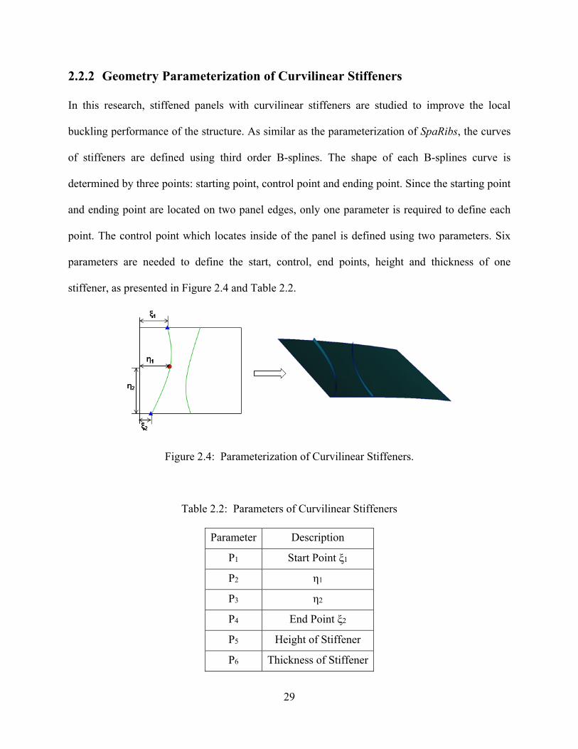
2.2.2 Geometry Parameterization of Curvilinear Stiffeners

In this research, stiffened panels with curvilinear stiffeners are studied to improve the local

buckling performance of the structure. As similar as the parameterization of SpaRibs, the curves

of stiffeners are defined using third order B-splines. The shape of each B-splines curve is

determined by three points: starting point, control point and ending point. Since the starting point

and ending point are located on two panel edges, only one parameter is required to define each

point. The control point which locates inside of the panel is defined using two parameters. Six

parameters are needed to define the start, control, end points, height and thickness of one

stiffener, as presented in Figure 2.4 and Table 2.2.

Figure 2.4: Parameterization of Curvilinear Stiffeners.

Table 2.2: Parameters of Curvilinear Stiffeners

Parameter Description

P1 Start Point ξ1

P2 η1

P3 η2

P4 End Point ξ2

P5 Height of Stiffener

P6 Thickness of Stiffener

30

2.3 Global-Local Optimization Framework

The MDO problem of aircraft wing structure can be defined mathematically as minimizing the

objective function f(x) , which is usually the structural weight, with respect to the design

variable vector x under the multidisciplinary constraints gi(x).

minx f(x)

Subject to gi (x1,x2,…,xn) ≤ gi

xj_L ≤ xj ≤ xj_U (2.12)

In Eq. 2.12, xj_L and xj_U are the lower and upper bounds on each of the design variables.

In this research, the objective of multidisciplinary optimization is to minimize the structural

weight subjected to constraints from several disciplines. The optimization problem is divided

into two coupled sub-systems: global wing optimization and local panel optimization. The

global-local multidisciplinary optimization framework, which consists of global wing

optimization module EBF3WingOpt and local panel optimization module EBF3PanelOpt, is

presented in Figure 2.5.

2.3.1 Global Wing Optimization

In the global wing optimization, both the topology of SpaRibs and the thicknesses of the wing

structural panels are optimized considering multidisciplinary constraints such as von Mises stress,

maximum displacement, flutter speed and buckling eigenvalue. A two-step optimization

approach is developed to reduce the complexity and improve the efficiency of global wing

optimization. The design variables are decomposed into two groups: shape variables that

determine the shape of SpaRibs, size variables that define the thickness of wing components.

Considering some shape variables, such as the number of spars or ribs, are not continuous, non-

31

gradient optimization methods are more suitable for searching the optimal topology design in the

global design space. In the first step of the optimization process, both the shape and size design

variables are optimized using particle swarm optimization (PSO), to minimize the weight of

wing structure. The wing topology design with minimum weight, which is obtained in the first

step optimization, is selected as the baseline design for the second step optimization. The second

step optimization with fixed wing internal topology design is carried out to optimize only the

size design variables. In this stage, gradient based optimization (GBO) method is used to refine

the thicknesses of wing skins and SpaRibs.

Figure 2.5: Global-Local Optimization Framework

32

In this research, MSC.PATRAN is utilized to create the geometry and finite element model of

the wing structure. The aerodynamic model is created using MSC.FlightLoads. The structural

and aerodynamic models are output as input files of MSC.NASTRAN for the aeroelasticity

analysis. The particle swarm optimization and gradient base optimization have been

implemented using MATLAB. The mentioned software are incorporated in the global

optimization framework EBF3WingOpt.

2.3.2 Local Panel Optimization

The goal of local panel optimization is to obtain a more precise structural design with minimum

weight by optimizing each panel bordered by spars and ribs, based on the design obtained

through global wing optimization. Static and linear buckling analyses are carried out for the local

panels using MSC.NASTRAN solution SOL105 that gives the first buckling eigenvalue as well

as the von Mises stress distribution in each panel.

Local panel optimization is implemented in EBF3PanelOpt. The flow diagram of local panel

optimization is presented in Figure 2.6. The aerodynamic forces applied on the wing structural

grid points are computed in static aeroelastic analysis using MSC.NASTRAN solution sequence

SOL144. The force fields are applied in the global static and buckling analysis, which generates

the displacement fields of the global model. The local panel models are defined by the

intersections of wing skins, spars and ribs. The finite element model of local panel and global

displacement fields are extracted from the global model. The applied loads in static and buckling

analysis of local panel are defined as enforced displacements applied at the edges of each panel.

Then static and buckling analyses are performed for the local panels to obtain the stress and

buckling results. Local panel design is optimized to satisfy the constraints applied on the first

33

buckling eigenvalue and the maximum von Mises stress. The global model is updated using the

optimized thicknesses of local panels. The new global displacement fields are computed using

the updated global model and applied on the local panels as enforced displacements to start the

next iteration of local panel optimization.

Figure 2.6: Flow Diagram of Local Panel Analysis.

Stiffened panel optimization with straight or curvilinear stiffeners has been integrated to improve

the buckling performance of local panels. Since buckling constraint is the critical constraint for

many local panels, there is significant potential to save the weight of local panels by adding

proper stiffeners. EBF3PanelOpt generates the geometry of stiffeners and meshes the stiffened

panel using a fine grid. The boundary conditions are defined using the displacements on the grid

nodes of panel edges. The fine grid of stiffened panel does not match with the grid of global

model. In order to solve that problem, a linear interpolation technology has been developed for

interpolating the displacements of global structural nodes onto the local panel edges. Static and

buckling analyses are included in the stiffened panel analysis. The panel is also optimized to

Analyze Global Model

Nastran SOL144

Extract the Global Displacement

Results

Create the Global Displacement

Field

Define the FEM of Local Panel

Create the Load Cases using Enforced Displacements on

Local Panel Edges

Define the Boundary of Local

Panel

Analyze the Local Model

Optimize Thickness of Local Panel

Update the Thicknesses in Global Model

Analyze Global Model

Nastran SOL105

Output Aerodynamic Forces

34

minimize the panel weight subject to stress and buckling constraints. Shape optimization of

stiffeners has been implemented to optimize the curvilinear stiffeners.

2.3.3 Integration of Global Wing and Local Panel Optimization

As shown in Figure 2.5, this global-local optimization procedure is an iterative process. After

local panel optimization, the optimized thicknesses of panels are substituted into the global wing

model. Then multidisciplinary analysis of the global wing model considering stress,

displacement, flutter and buckling constraints is carried out to generate the new displacement

results. The new global displacement fields are interpolated onto the edges of local panels as

boundary conditions to start the next iteration of the local panel optimization. The details of the

integrated global-local optimization procedure will be discussed in Chapter 5.

The global-local optimization framework has been implemented by incorporating

EBF3WingOpt for global wing optimization and EBF3PanelOpt for local panel optimization.

The framework is developed using MATLAB programming to integrate MSC.PATRAN for

pre/post processing, MSC.NASTRAN for finite element analysis, and Python code of

EBF3PanelOpt.

35

2.4 Summary

In this chapter, the integration of multidisciplinary analysis and geometry parameterization are

discussed for the global wing optimization and local panel optimization. The global wing

optimization is implemented in EBF3WingOpt. The local panel optimization procedure

EBF3PanelOpt is also described. The global-local optimization framework has been developed

to integrate the optimization software package EBF3WingOpt and EBF3PanelOpt. Multiple

disciplines like static aeroelasticity, buckling, and dynamic flutter are considered in the

optimization process. The geometry of curvilinear spars, ribs, and stiffeners are parameterized

and constructed automatically by the optimization software package. The optimization

framework is not only developed for a particular aircraft wing but also can be easily generalized

for the design of other aircraft wings by changing the geometry parameters.

36

Chapter 3

Global Wing Optimization: EBF3WingOpt

In this chapter, the details of the global wing optimization framework EBF3WingOpt are

discussed. The aircraft wing optimization has been applied to a concept supersonic wing Boeing

High Speed Commercial Transport aircraft (Boeing HSCT) and subsonic wing NASA Common

Research Model (NASA CRM). The advantages of using curvilinear spars and ribs, termed

SpaRibs, are investigated to design aircraft wing-box in comparison to the use of classic design

concepts that employ straight spars and ribs. This optimization scheme performs both the sizing

and the shaping of the wing internal structure, connecting the geometry modeling software

MSC.PATRAN and finite element analysis software MSC.NASTRAN.

37

3.1 Optimization of Boeing N+2 HSCT Wing

3.1.1 Boeing N+2 HSCT Wing Description

The Boeing HSCT aircraft is characterized by an 86.1 ft wing span and a fuselage length of

about 154 ft; 30 passengers can be transported at a cruise velocity equivalent to Mach 1.6 at an

altitude of 50,000 ft for a maximum range of 3200nm. The baseline aircraft layout is presented in

Figure 3.1 [82]. The wing, tail and fuselage structures are specified as fabricated from a titanium

alloy material, while the secondary structures and control surfaces are fabricated from

honeycomb and composite materials. The yield stress of the titanium alloy chosen for the design

is 110,000 psi. Titanium alloy physical characteristics widely change depending on the alloy

composition and thermal treatments. In particular, the yield stress can vary from about 100,000

psi to over 200,000 psi. In absence of more precise indications, a lower grade alloy has been

chosen as reference for the design to avoid contamination of the results due to the “optimistic”

estimation of the material properties. In the baseline aircraft design, straight spars and ribs are

used for the wing and tail internal structure which is outlined in Figure 3.2.

Figure 3.3 shows the flight envelope of Boeing N+2 HSCT aircraft [83]. The aircraft cruises at a

subsonic velocity Mach 0.836 if the altitude is between 20,000 ft and 35,000 ft, or at a

supersonic velocity Mach 1.6 if the altitude is above 40,000ft. In this research, two flight

conditions are concerned in the optimization: Mach 0.836 at 20,000 ft and Mach 1.6 at 40,000 ft.

38

Figure 3.1: Boeing N+2 HSCT Aircraft Concept.

Figure 3.2: Boeing N+2 HSCT Aircraft Structural Configuration. (Chen et al. 2010 [83])

39

Figure 3.3: Flight Envelop of Boeing HSCT Aircraft Concept. (Chen et al. 2010 [83])

3.1.2 Optimization Procedure of Boeing N+2 HSCT Wing

The N+2 supersonic aircraft concept developed by Boeing was optimized using EBF3WingOpt

framework by Virginia Tech unitized structures group. The internal structure layout is replaced

by a new layout characterized by curvilinear SpaRibs. The optimization of the structural weight

was conducted under structural stress and subsonic and supersonic flutter constraints. The

optimization includes the re-design of the load bearing structure of the wing and of the tail; the

fuselage structure, the control surfaces and the wing and tail tips are not optimized using

EBF3WingOpt and are kept fixed throughout the process. The optimization framework

EBF3WingOpt developed for Boeing N+2 wing includes a geometry modeling module, a static

aeroelastic analysis module, an flutter analysis module and an optimization module.

The geometry parameterization has been implemented in the EBF3WingOpt optimization

framework using MSC.PATRAN session file. The geometry and finite element model of Boeing

HSCT wing internal structure are defined by a set of design variables. An example of wing

40

internal SpaRibs layout automatically generated using MSC.PATRAN is presented in Figure 3.4.

The wing internal topology is divided into 14 smaller wingboxes. SpaRibs layout is defined by

Linked Shape Method in each wingbox. Therefore the wing internal SpaRibs layout is defined

using 53 shape variables. The details of the geometry definition of Boeing HSCT wing has been

presented in Ref. [84].

Figure 3.4: Example of Internal Wing Structure Configuration Generated with EBF3WingOpt

The static aeroelastic analysis module computes the flight loads and the associated stresses for

multiple flight conditions. The flight loads and structural stress calculation are carried out by

MSC.Nastran. There are five maneuvers concerned in the optimization: 2.5g pull up, -0.5g push

over and roll at Mach 0.836 and 20,000 ft altitude, 1.2 g pull up and 1.5g pitch up at Mach 1.6

and 40,000 ft altitude.

The stress response of the wing structure is evaluated using an aggregated stress approximation.

The stress constraint is formalized using the modified Kreisselmeier-Steinhauser criterion,

following the relation:

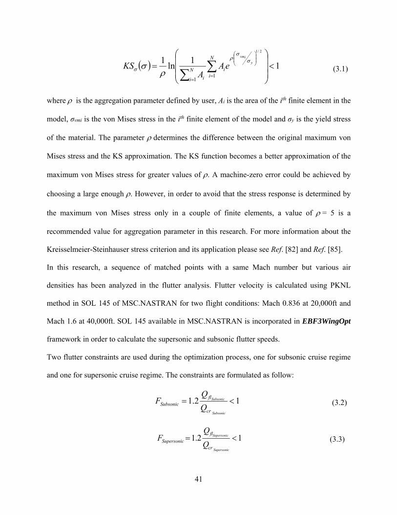
41

11

ln1

11

2/1

N

iiN

i i

y

ivm

eAA

KS

(3.1)

where is the aggregation parameter defined by user, Ai is the area of the ith finite element in the

model, σvmi is the von Mises stress in the ith finite element of the model and σy is the yield stress

of the material. The parameter determines the difference between the original maximum von

Mises stress and the KS approximation. The KS function becomes a better approximation of the

maximum von Mises stress for greater values of . A machine-zero error could be achieved by

choosing a large enough . However, in order to avoid that the stress response is determined by

the maximum von Mises stress only in a couple of finite elements, a value of = 5 is a

recommended value for aggregation parameter in this research. For more information about the

Kreisselmeier-Steinhauser stress criterion and its application please see Ref. [82] and Ref. [85].

In this research, a sequence of matched points with a same Mach number but various air

densities has been analyzed in the flutter analysis. Flutter velocity is calculated using PKNL

method in SOL 145 of MSC.NASTRAN for two flight conditions: Mach 0.836 at 20,000ft and

Mach 1.6 at 40,000ft. SOL 145 available in MSC.NASTRAN is incorporated in EBF3WingOpt

framework in order to calculate the supersonic and subsonic flutter speeds.

Two flutter constraints are used during the optimization process, one for subsonic cruise regime

and one for supersonic cruise regime. The constraints are formulated as follow:

12.1 Subsonic

Subsonic

cr

flSubsonic Q

QF (3.2)

12.1 Supersonic

Supersonic

cr

fl

Supersonic Q

QF (3.3)

42

where Qcr is the critical dynamic pressure computed using MSC.NASTRAN and Qfl is the

dynamic pressure at the two flight conditions. A safety factor of 1.2 is also applied on the flutter

velocities. If the flutter analysis shows that the critical dynamic pressure value is outside the

range investigated the flutter constraint value is considered to be zero. From Ref. [83] the

velocities for subsonic and supersonic flight conditions are chosen to be 867 ft/sec at 20,000 ft

(M = 0.836) and 1782 ft/sec at 40,000 ft (M = 1.6), respectively. The corresponding dynamic

pressure values are 3.31 psi and 6.19 psi respectively.

The aerodynamic model of Boeing HSCT wing is defined using MSC.FlightLoads. As shown in

Figure 3.5, the aerodynamic surface consists of 840 aerodynamic boxes. The aerodynamic loads

are interpolated onto the spline nodes, which locate at the intersection of upper wing skin and

SpaRibs, to compute the structural deformation and stress. Some grid points in the control

surfaces, wing tip and tail tip, are also selected as spline nodes for transforming the aerodynamic

loads onto those regions. The spline nodes are shown in Figure 3.6.

Figure 3.5: Aerodynamic Elements of Boeing HSCT Wing

43

Figure 3.6: Spline Nodes in Boeing HSCT Wing

In order to reduce the complexity of the optimization problem, the design variables of the Boeing

N+2 wing are decomposed into two groups: topology variables that define the topology of wing

internal structure, and size variables which determine the thicknesses of wing components. The

EBF3WingOpt framework incorporates both topology optimization and size optimization for the

Boeing N+2 supersonic wing. The optimal topology configuration of wing internal structure is

computed in the first optimization step; the optimal thicknesses of the wing skin panels and

SpaRibs are computed with the fixed optimal topology of wing internal structure in the second

optimization step. The structural weight is minimized in each step of the optimization subject to

the strength and flutter constraints. The optimization framework is presented in Figure 3.7. The

topology optimization requires both topology and size design variables to be specified for

computing the stress and flutter responses of the aircraft structure. At this stage, the topology

design variable vector and two thickness variables are used to generate an aircraft configuration,

including the geometry definition of the SpaRibs and wing skins and the finite element model for

44

aerodynamic and structural analysis. Constraints are prescribed on the number and shape

variables of SpaRibs to be placed in the wing structure. If the number of SpaRibs is determined,

the value of the corresponding design variables could be fixed and the optimizer would find the

best shape of the SpaRibs for that particular requirement.

The wing components are decomposed into 31 groups. The thickness of the structural

components is optimized using the 31 size variables in the second step with the given topology

configuration obtained in the first step. The details of the wing components decomposition is

discussed in the chapter 3.1.4.

Figure 3.7: Global Optimization Framework for Boeing N+2 HSCT Wing

The optimization of topology and size design variables is carried out using particle swarm

optimization method. Once the responses are computed the optimizer checks the convergence

45

criterion of the optimization method used and eventually restarts the process with a new design

variables vector, if the convergence in not achieved. The topology and size loops are executed

sequentially and convergence must be achieved in both steps separately. The final output of the

optimization process is a wing structure with optimal topology and optimal thickness, for that

particular configuration of SpaRibs, and that satisfies both strength and flutter constraints.

3.1.3 Baseline Boeing N+2 HSCT Configuration

This baseline aircraft configuration was optimized under strength and flutter constraints by the

Boeing Company. The results are summarized in Chen et al. 2010 [83]. As shown in Table 3.1,

the weight of the load bearing structure optimized to satisfy only the strength constraint is 39,305

lbs. If the flutter constraint is considered, the weight of the structure increases by 18.5%.

Table 3.1: Weight Summary for Boeing N+2 Aircraft Concept (Chen et al. 2010 [83]).

Strength Optimization Strength and Flutter Optimization

Wing Structural Weight (lb) 39,305 46,587

Weight of Re-Design Portion (lb) 12,780 16,050

The wing structural weight presented in reference paper [83] refers to the whole structure of the

aircraft concept developed by Boeing. This includes the wing, the tail and the fuselage. The

weight of baseline design is subdivided as follow: wing-tail assembly 25,560 lbs, fuselage

assembly 13,745 lbs. The EBF3WingOpt optimization framework is only applied to re-design

part of the wing and the tail structure. For consistency the data relative to the half portion of the

structure re-designed during the optimization process are also presented in Table 3.1. The

weight of re-design portion refers to the half structure presented in Figure 3.4. The mass of the

46

structure subjected only to the strength constraint is computed from the finite element model

provided by Boeing, using MSC.PATRAN mass estimator. The weight of a half re-design

portion was increased from 12,780 lb to 16,050 lb in strength and flutter optimization.

3.1.4 Optimization Results of Boeing N+2 HSCT Aircraft

This aircraft configuration is optimized and subjected to strength and flutter constraints in

EBF3WingOpt. The strength constraints are computed for different flight conditions as

prescribed by Boeing. The optimal weight of the portion of the structure that was actually

optimized is presented in Table 3.2. The mass refers to the half structure presented in Figure 3.8.

Figure 3.8: Finite Element Mesh of the Portion of the Re-designed Structure

Table 3.2: Mass Summary for Boeing N+2 Aircraft Concept Optimized with SpaRibs.

Strength and Flutter Optimization

Optimal Weight (lb) 12,340

47

Table 3.3 and Table 3.4 present the constraint coefficients computed according to the relations

presented above. The coefficients refer to the configuration shown in Figure 3.8. The stress

constraints are satisfied in all of the five flight conditions. Flutter does not occur in the flight

range investigated therefore the flutter constraint coefficients are zero. This means that the

structure actually flutters outside the flight envelope and the flutter velocity and critical dynamic

pressure requirements are satisfied.

Table 3.3: Kreisselmeier-Steinhauser Coefficients for Different Flight Conditions

Maneuver KSσ(σ)

2.5G Pull Up at M = 0.836 0.89

1.2G Pull Up at M = 1.6 0.34

-0.5G Push Over at M = 0.836 0.17

Roll at M = 0.836 0.53

1.5G Pitch Up at M = 1.6 0.33

Table 3.4: Flutter Constraint Coefficients of Optimal Configuration.

FSubsonic 0.0

FSupersonic 0.0

The first step of the optimization process is to find the optimal topology design of the SpaRibs.

This task involves the use of 53 design variables which define number of SpaRibs required and

their curvilinear shape. The optimum topology configuration computed at this stage is shown in

48

Figure 3.9 along with the baseline structure for comparison. The optimized structure is

characterized by a higher number of internal elements in every section of the wing.

Figure 3.9: Optimum Topology Computed at the First Optimization Step.

The second phase of the optimization process is the sizing of the internal components and the

skin panels. This task includes 31 size design variables to define the thickness of wing structure.

The optimal size of re-designed wing components is presented in Figure 3.10. The maximum

component thickness is reduced to about 0.3 inches from the 1.1 inches of the baseline. In

general a significant thickness reduction of the skin panels is observed. The reduction is more

49

pronounced in the outer, center and forward portion of the wing structure. The forward wing is

characterized by thicker SpaRibs.

Figure 3.10: Thickness Distribution of the Optimized Structure (in).

The static aeroelastic analysis is performed for every load case listed in Table 3.4. The most

severe maneuver from the stress point of view is the 2.5 G pull-up maneuver at Mach 0.836 and

20,000 ft altitude. The von Mises stress distribution in the re-design region of wing structure is

plotted in Figure 3.11.

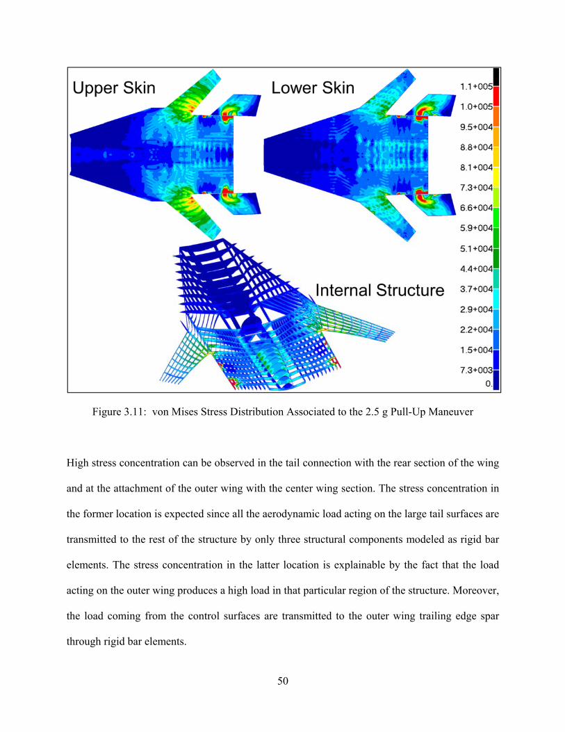
50

Figure 3.11: von Mises Stress Distribution Associated to the 2.5 g Pull-Up Maneuver

High stress concentration can be observed in the tail connection with the rear section of the wing

and at the attachment of the outer wing with the center wing section. The stress concentration in

the former location is expected since all the aerodynamic load acting on the large tail surfaces are

transmitted to the rest of the structure by only three structural components modeled as rigid bar

elements. The stress concentration in the latter location is explainable by the fact that the load

acting on the outer wing produces a high load in that particular region of the structure. Moreover,

the load coming from the control surfaces are transmitted to the outer wing trailing edge spar

through rigid bar elements.

51

The high stress regions amount to only about 2% of the total wing surface therefore can be

considered local effects caused by the use of the rigid bar elements to connect the various parts

of the structure. A more accurate modeling of the structure and a localized optimization should

solve the issue effectively. The forward section of the wing is practically unstressed for this

flight maneuver.

Figure 3.12 shows the von Mises stress distribution for the remaining maneuvers. The most

critical maneuver, after the 2.5 g pull-up at Mach 0.836, is the roll at Mach 0.836 at a roll rate of

25 degrees per second. This kind of maneuver generates an asymmetric aerodynamic pressure

distribution on the aircraft. The portions of the wing characterized by high stress are the tail-wing

connection and the outer wing-center wing attachment, as observed in the previous case. The 1.2

g pull-up maneuver and the 1.5 g pitch-up maneuver at Mach number equal to 1.6 have similar

stress distribution with higher stresses localized in the tail-wing connection region. Finally the

push over maneuver at Mach number equal to 0.836 and load factor equal to -0.5 is characterized

by a very low stress level throughout the whole structure. In conclusion the strength design is

driven by the pull-up maneuver at 2.5 g and by the roll maneuver at Mach number equal to

0.836. The most critical regions of the structure, from the stress point of view, are the tail-wing

connection region, tail surfaces, the rear wing and the outer wing.

52

Figure 3.12: von Mises Stress of the Aircraft Structure

Clockwise from pitch-the Top Left Corner: 25 deg/sec Roll at Mach = 0.836, 1.2 g Pull-Up at Mach = 1.6, 1.5 g

Pitch-Up at Mach = 1.6, -0.5 g Push Over at Mach = 0.836

The flutter analysis is performed using the PKNL method available in MSC.NASTRAN. The

results show that flutter does not occur for the flight conditions studied. In particular, the flutter

modes damping is always negative for the range of dynamic pressure considered. Figure 3.13

shows the structural damping as function of the dynamic pressure for the subsonic and

supersonic regimes, respectively. The damping value is always negative therefore flutter does not

occur.

53

Figure 3.13: Flutter Analysis Results

The baseline and the SpaRibs-optimized structure performance are compared in Table 3.5. The

use of the SpaRibs allows for a mass reduction of the structure 22.6%. Furthermore both the

subsonic and supersonic flutter constraints are met.

Table 3.5: Optimized Structure Performance Compared.

Baseline Optimized with SpaRibs

Weight (lb) 16,050 12,430 (22.6% Reduction)

Stress Constraints Satisfied Satisfied

Subsonic Flutter Not Satisfied Satisfied

Supersonic Flutter Satisfied Satisfied

54

3.2 Optimization of NASA Common Research Model

3.2.1 NASA Common Research Model (CRM) Wing Description

The transport aircraft wing configuration NASA Common Research Model (CRM) is studied in

this research. The CRM wing is a cantilever wing with a full wingspan of 192.8 ft, aspect-ratio of

nine, a taper-ratio of 0.275 [86]. An example of CRM wing layout is shown in Figure 3.14. The

wing can be divided into the inner wing and the outer wing sections at the junction located at 37%

semi-span. An aerodynamic model of the CRM wing is created using MSC.PATRAN for the

aerodynamic load calculation. Figure 3.15 shows the aerodynamic model of CRM wing that

consists of three aerodynamic lifting surfaces and 500 aerodynamic boxes. The spline nodes

shown in Figure 3.16 are selected at the intersections of top wing skin and SpaRibs. A minimum

distance requirement of 20 inch is applied on the adjacent spline nodes to avoid selecting too

many spline nodes.

Figure 3.14: Example of NASA Common Research Model

55

Figure 3.15: Aerodynamic Elements of NASA CRM Wing

Figure 3.16: Example of Spline Nodes in NASA CRM Wing

3.2.2 Design Variables in Optimization of Subsonic CRM Wing

In the global/local optimization, the topology of the stiffening members and the thicknesses of

the panels are optimized, and the outer model line (OML) is not changed in this research.

Curvilinear SpaRibs are defined in each wing section and the C0 continuity is enforced on the

56

junction of the each two adjacent sections. The CRM wing internal structure is generated using

24 design variables with the linked shape method [80]. The details of those shape design

variables of the spars or ribs in different wing sections are given in Table 3.6 and Table 3.7. The

CRM wing is modeled using aluminum alloy 2024-T3 and its material properties are given in

Table 3.8.

Table 3.6: Shape Design Variables

SpaRibs Design Variables

Front and Rear Spar DV1 ~ DV2

Spars in Inner Wing DV3 ~ DV8

Ribs in Inner Wing DV9 ~ DV14

Spars in Outer Wing DV15 ~ DV18

Ribs in Outer Wing DV19 ~ DV24

Table 3.7: Boundary of Shape Design Variables of Spars and Ribs

Parameter Description Lower Bound Upper Bound

P1 Number of SpaRibs 2 20

P2 η1 0.1 0.9

P3 η2 0.1 0.9

P4 ξ11/ ξ12 0.25 4

P5 ξ21/ ξ22 0.25 4

P6 ξ31/ ξ32 0.25 4

57

Table 3.8: Aluminum Alloy 2024-T3 Mechanical Properties

Density (lb/in3) 0.1

Modulus of Elasticity(ksi) 10,600

Possion’s Ratio 0.33

Yield Stress (ksi) 40

Thicknesses of wing skins and SpaRibs are specified by non-uniform thickness fields. In this

study, non-uniform fields are defined using linear or nonlinear function of the Y-coordinate. Two

design variable values are needed to create a linear function. One design variable is the thickness

of the skin at the wing root. The other design variable specifies the thickness of panels at the

wing tip. Four thickness fields were specified for the four subgroups of wing structure

components: upper skin, lower skin, spars and ribs. In some cases, nonlinear thickness fields are

more efficient than the linear thickness fields when it comes to the structural weight saving. The

motivation of such a nonlinear function comes from that the high stress region of design with

linear thickness fields locates around the junction of the outer wing and inner wings, while the

skin stresses in the wing tip and wing root region are relatively low. Therefore a straightforward

idea is to increase the skin thickness in such high stress region while reducing the skin thickness

in the low stress region. In this study, a combination of quadratic and triangular thickness fields

has been studied. An example of the nonlinear function is shown in Figure 3.17. In the quadratic

function, thickness decreases from the wing root region to the wing tip region faster than it does

in linear function. The thickness in the junction region is increased by adding the triangular

function and the quadratic function. The size design variables in the CRM wing optimization is

presented in Table 3.9.

58

Figure 3.17: Nonlinear Thickness Fields

Table 3.9: Size Design Variables

Wing Components Linear Fields Non-linear

Spars DV25 ~ DV26 DV25 ~ DV27

Ribs DV27 ~ DV28 DV28 ~ DV30

Top Wing Skin DV29 ~ DV30 DV31 ~ DV33

Bottom Wing Skin DV31 ~ DV32 DV34 ~ DV36

3.2.3 Optimization Procedure of NASA CRM Wing

In this section global optimization is demonstrated for NASA common research model (CRM)

considering stress, deformation and flutter constraints. The static aeroelastic analysis is

implemented using sequence SOL144 in MSC.NASTRAN. An aerodynamic model of the wing

is created to provide aerodynamic loads for static aeroelasic analysis using doublet-lattice

method for subsonic problems. The aerodynamic grid nodes do not coincide with structural grids.

59

A set of splines has been defined for transferring the aerodynamic forces to the structure and

transferring displacements from structure to aerodynamic model. Fixed boundary conditions are

applied on the CRM wing root. Five flight conditions are defined using angle of attack of -2, 0, 2,

4, 6 degrees respectively, and cruise Mach number of M=0.8 at altitude of 35,000 ft.

The stress constraint is evaluated using Kreisselmeier-Steinhauser (KS) criterion. For this

cantilever wing model, structural deformation can be measured using the displacement at the

wing tip. Displacement constraint is defined using Eq. 3.4. (uz)max is maximum vertical

displacement at wing tip, b is semi-span of CRM wing.

max( )1

12%zu

b

(3.4)

Twist angle constraint is defined using the vertical displacements at the wing tip. As shown in Eq.

3.5, the twist angle at wing tip should not exceed 6 degrees. (uz)+max and (uz)-

max are the

maximum vertical displacements in positive and negative direction of z-coordinate, respectively.

Here, Ctip is the chord length at wing tip.

Twist Angle at Wing Tip = 180

6z zmax max

tip

u u

c

(3.5)

Flutter analysis is carried out using PKNL method in solution 145 of MSC NASTRAN. The

flutter constraint is defined using the dynamic pressure Qc at cruise Mach number of M = 0.85

and at altitude of 35,000 ft. A sequence of matched points with a same Mach number of 0.85 but

various air densities are included in the flutter analysis. Twenty modes are included in the flutter

analysis of the CRM wing. In Eq. 3.6, a safety factor of 1.2 is applied to the flutter constraint.

QFlutter ≥ 1.2 Qc (3.6)

Number of eigenvalues extracted in eigenvalue analysis is a user defined parameter in flutter

analysis. For a given structure, some mode shapes result from local vibration but not global level

60

vibration. In order to obtain a reliable flutter result, enough number of global modes, such as

bending and torsional modes, should be included in flutter analysis. Constraints of Natural

frequencies and mode shapes are considered in the multidisciplinary optimization. The constraint

for first natural frequency is enforced as in Eq. 3.7.

f1 ≥ 1.0 Hz (3.7)

In the eigenvalue calculation the eigenvectors are normalized using maximum displacement. In

that case the generalized mass of each mode can be used to classify whether a mode is global or

local. If the generalized mass of a certain mode is greater than 10% of maximum generalized

mass of all the modes included in the eigenvalue analysis, the mode is considered to be a global

mode. Based on that criterion, the constraint on number of global modes is defined in Eq. 3.8.

Number of Global Modes ≥ 5 (3.8)

3.2.4 Optimization Results of Common Research Model

The CRM wing configuration is optimized under the above constraints in the global optimization

framework using a two-step optimization approach. The topology of SpaRibs and thicknesses of

panels are optimized in the first step optimization. The size design variables are refined in the

second step optimization. The optimization is carried out using linear thickness fields or

nonlinear thickness fields. The comparison of the results of the two schemes has been

summarized in Table 3.10. The maximum von Mises stress is the active constraint in both of the

two cases. The structural weight has been reduced 18.5% using nonlinear thickness fields

compared with the results obtain from linear thickness fields approach. Figure 3.18 and Figure

3.19 show the optimal thickness fields and von Mises stress distribution of optimal designs,

respectively. In the case using linear thickness fields, thickness decreased from the wing root to

61

the wing tip, which induced a high stress region at the junction of outer wing and inner wing. In

the nonlinear thickness fields design, that high stress region has been divided into two regions,

which causes a large area of the wing is close to full stressed state. The reason is that as

compared to the linear thickness fields, in the nonlinear thickness fields case, the thickness in the

junction region has been increased, and thicknesses in both the wing root and tip region are

reduced. The comparison shows that for the stress dominated optimization problem, the

nonlinear thickness scheme is much more efficient than linear thickness fields scheme. For the

design optimized using nonlinear thickness fields, the stress responses are presented in Table

3.11, and optimal topology of SpaRibs is shown in Figure 3.20. Modal analysis is carried out to

output the mode shapes of the first 20 flexible modes. Eight of the 20 modes are global models.

The global mode shapes of the CRM wing are shown in Figure 3.21.

Table 3.10: Comparison of Optimal Designs using Different Thickness Fields

Optimal Design Structural Weight Maximum von Mises Stress in KS Criterion

Thickness with Linear Fields 9182.4 lbs 0.999

Thickness with Nonlinear Fields 7481.1 lbs 0.999

Figure 3.18: Optimized Thickness Fields

62

Figure 3.19: von Mises Stress Distribution

Table 3.11: Constraints of Global Optimal Design with Nonlinear Thickness Fields

Constraints Optimal Design Low Bound Up Bound

M0.85 -2 Degree KS 0.237 NA 1

M0.85 0 Degree KS 0.039 NA 1

M0.85 2 Degree KS 0.265 NA 1

M0.85 4 Degree KS 0.628 NA 1

M0.85 6 Degree KS 0.999 NA 1

Max Displacement/Semispan 0.106 NA 0.125

Max Twist Angle (Degree) 3.96 NA 6

First Natural Frequancy (Hz) 1.21 1.0 NA

Number of Global Modes 5 5 NA

Flutter Dynamic Pressure (psi) 6.78 2.1 NA

(a) Nonlinear Thickness Fields (b) Linear Thickness Fields

63

Figure 3.20: Optimal Design Using Nonlinear Thickness Fields

Figure 3.21: Global Modes of Optimal CRM Wing

64

3.2.5 Pre-stressed Modes and Unstressed Modes in Flutter Analysis

In this research, the effect of pre-stressed mode shapes on the flutter velocity is studied. Flutter

analysis of the CRM model is performed in two cases using different mode shapes: the mode

shapes of stressed or unstressed wing. The pre-stressed mode shapes are calculated in pre-

stressed modal analysis, in which case the applied loads are computed by static aeroelastic

analysis using MSC.NASTRAN solution SOL144. Then the pre-stressed modes are imported

into flutter analysis which is carried out using NASTRAN solution SOL145. In that analysis,

pre-stressed mode shapes are computed using the load case defined by the angle of attack of 6

degrees. The dynamic pressure vs. damping curves of the two cases in Figure 3.22 show that the

flutter dynamic pressure of pre-stressed mode case is 7.14 psi which is about 5% higher than

flutter dynamic pressure of 6.78 psi in the unstressed mode case, both of the two cases satisfy

flutter constraint. Figure 3.23 shows the flutter frequencies computed by the un-stressed and pre-

stressed flutter analyses.

Figure 3.22: Flutter Dynamic Pressure

65

Figure 3.23: Flutter Frequency

3.3 Summary

In this chapter, the aircraft wing optimization framework EBF3WingOpt has been applied to a

concept supersonic wing Boeing High Speed Commercial Transport aircraft (Boeing HSCT) and

subsonic wing NASA Common Research Model (NASA CRM). The global wing optimization

tool (EBF3WingOpt) has proven its efficiency in optimizing the weight of a wing box using

SpaRibs as compared to using the classic straight spars and ribs. The method has been applied

with success for designing the complex wing box configurations. The geometry of SpaRibs is

parameterized using Linked Shape Method. Both topology optimization and size optimization are

performed for the Boeing HSCT wing and NASA CRM wing subject to von Mises stress and

flutter constraints. In the trim analysis and flight load calculation, multiple flight conditions are

considered. The internal structure of Boeing HSCT is optimized subjected to stress and flutter

constraints and multiple flight conditions. The baseline N+2 Boeing configuration is at first

described and subsequently compared with the design optimized using EBF3WingOpt

framework. The results show that the use of the SpaRibs allows for the reduction of the aircraft’s

66

primary structure weight without violating the constraints. The results show a reduction of the

weight of the wing/tail load bearing structure of about 20%. The internal structure of NASA

CRM wing is optimized using curvilinear spars and ribs while considering stress, displacement

and flutter constraints. The thickness distribution of CRM wing is optimized using linear

thickness fields and non-linear thickness fields. The comparison shows the advantage of non-

linear thickness fields in the wing weight reduction. The pre-stressed flutter analysis is

implemented for the optimal CRM design obtained in global wing optimization. The result

shows the pre-stressed flutter dynamic pressure is 5% higher than the un-stressed flutter dynamic

pressure.

67

Chapter 4

EBF3PanelOpt: Un-Stiffened Panel Optimization

Plenty of previous researches have shown that the panel buckling is a crucial problem in aircraft

structural design. In this chapter, local panel optimization framework EBF3PanelOpt is

developed to minimize the structural weight by optimizing the local panels of wing structure.

The un-stiffened panel optimization is implemented and applied on the NASA common research

model (CRM) wing. The panel thicknesses are optimized using the results of stress and buckling

analyses to minimize the wing weight subject to strength and buckling constraints.

68

4.1 Local Panel Optimization Procedure of CRM Wing

CRM wing is optimized using un-stiffened panels while considering stress, displacement, flutter

and buckling constraints. As shown in Figure 4.1, a CRM design with 3 straight spars and 37

straight ribs, provided to us by NASA, is decomposed into local panels bordered by spars and

ribs. Figure 4.2 presents the thickness and stress distributions, and fundamental buckling mode

shape of this CRM design, which has been optimized subject to stress and flutter constraints, but

without considering buckling constraint. The corresponding buckling eigenvalue of the buckling

mode shape shown in Figure 4.2 is only 0.141, that means the CRM design violates the buckling

constraint. In the local panel optimization, the topology of CRM wing structure is not optimized.

The un-stiffened panel optimization is performed based on this CRM design to make it satisfy

buckling constraint.

Figure 4.1: CRM Design with 37 Straight Ribs Provided by NASA

69

(a) Thickness (b) von Mises Stress (c) Fundamental Buckling Mode Shape (AOA 6o)

Figure 4.2: Results of Baseline CRM Design with 37 Straight Ribs

Two flight conditions are considered in the optimization: angle of attack equals -2 or 6 degrees.

In the local panel optimization, the stress and buckling constraints should be satisfied in both of

the two load cases. The aerodynamic forces applied on the wing structure are computed in static

aeroelastic analysis using MSC.NASTRAN solution SOL144. The force fields are multiplied by

a safety factor of 1.15 and applied on the global wing model for the static and buckling analysis,

which generates the displacement fields of the wing model. The buckling constraint is defined in

Eq. 4.1:

λp > 1.0 (4.1)

where λp is fundamental buckling eigenvalue. If the λp is greater than 1, it means the critical

buckling load is greater than the applied load.

The process of un-stiffened panel optimization is illustrated in Figure 4.3. In the local panel

optimization, the buckling analyses are carried out for the global wing and local panels. Each

local panel is optimized by a uniform thickness to instead of the thickness fields that used in the

baseline CRM wing model. The thicknesses of the local panels are optimized to increase the

buckling eigenvalue to be greater than 1. Then the global model is updated using the optimized

70

panel thicknesses in each optimization cycle. The convergence criterion, as shown in Eq. 4.2, is

defined using the number of panels that violate the stress or buckling constraints, and the relative

change of total wing weight in the ith optimization cycle.

Number of Panels Violate Constraint < 5

| |

1% (4.2)

Figure 4.3: Local Panel Optimization Procedure

In the local panel optimization, the boundary conditions of local panels are defined using the

translational displacements of the grid points on the panel edges, which are not exactly the same

as the actual boundary constraints applied on the local panels in the global wing model.

Therefore, even if all the local panels satisfy the local buckling constraints, the buckling

eigenvalue of the global wing usually does not satisfy the global buckling constraint. A panel

71

thickness modification process is performed based on the wing design which satisfies the

convergence criterion of the iterative local panel optimization. The detailed process of panel

thickness modification is described in Figure 4.4. Buckling eigenvectors of the first m buckling

modes of the global wing are computed and normalized to the maximum eigenvector using

MSC.NASTRAN. The grid points with the maximum buckling eigenvectors (vmax = 1.0) locate

in the buckled panels. As shown in Figure 4.4, the maximum buckling eigenvector of the 1st

buckling mode is found in the local panel i1. If the fundamental buckling eigenvalue λp of the

global wing is less than 1, the thicknesses of the buckled panels should be optimized to satisfy

the buckling constraints. The optimal wing design which satisfies the global buckling constraints

can be obtained through the iterative panel thickness modification process.

Figure 4.4: Modification of Local Panel Thickness

72

4.2 Buckling Analysis of Local Panel

In the buckling analysis of panel, boundary conditions are usually defined using the forces or

displacements that applied on the panel edges. The local panels in the CRM wing are connected

to the spars or ribs at the panel edges. If the thickness of a certain panel is changed, the forces

applied on that panel edges may change dramatically. However, because the support of spars and

ribs, the displacements at the panel edges only change a little bit. Therefore displacements are

selected as boundary conditions and applied on the panel edges in the local panel optimization.

The displacement data of the grid points on panel edges are extracted from the displacement

fields of the global wing. The displacement vector of a grid point consists of six components:

three translational displacements and three rotational displacements. Two boundary conditions

have been considered: only apply translational displacements on panel edges (termed Case 1), or

apply both translational and rotational displacements (termed Case 2). The Case 1 is equivalent

to assuming that the panel edges are constrained by simple supports. The Case 2 means the panel

edges are clamped. The static and buckling analyses are performed for the panel with the two

types of boundary conditions. The buckling analysis is also carried out for the global CRM wing.

Local buckling modes can be found in several local panels from the buckling results of the global

wing. A local buckling mode shape is extracted from the global wing model and shown in Figure

4.6 (termed Case 3), in comparison to the fundamental buckling mode shapes of the same panel

computed in Case 1 and Case 2. The corresponding buckling eigenvalues are compared in Table

4.1. The buckling eigenvalue of case 1 is closer to the buckling result of the global wing.

Therefore, the boundary conditions in buckling analysis of local panels should be defined using

the translational displacements at the panel edges.

73

Table 4.1: Fundamental Buckling Eigenvalues of Local Panel

Case 1 Case 2 Case 3

1st Buckling Eigenvalue 1.01 1.69 1.08

Figure 4.5: Boundary Conditions in Local Panel Analysis

Figure 4.6: 1st Buckling Mode Shape of Local Panel with Various Boundary Conditions

74

4.3 Panel Thickness Optimization

For the thin rectangular flat plate with compressive loads applied on two opposite edges, the

critical buckling stress can be computed using the analytic solution given by the following

formula [47, 53].

(4.3)

where is the plate thickness, and is the length of the panel edges with compressive

loads. k is a constant depends upon the aspect ratio of the panel being investigated. Thickness of

each local panel is optimized using the first buckling eigenvalue and maximum von Mises stress

in full stress optimization scheme as shown in Eq. 4.4. topt1 is the optimized thickness of local

panel considering maximum von Mises stress (σvm)max in that panel. topt2 is the optimized

thickness using first buckling eigenvalue λp of that panel. Topt is the optimized thickness of local

panel.

topt1 = t0 (σvm)max / σy

topt2 = t0 (1/ λp)1/2

topt = max(topt1 , topt2 ) (4.4)

The local panel optimization is an iterative process. In each optimization cycle, the local panel

thicknesses are optimized. Then the global finite element model needs to be updated using the

new panel thicknesses. Displacement fields of global model are computed by the aerodynamic

and static analyses. The thicknesses and boundary conditions of local panels are changed in each

optimization cycle, which causes oscillation of panel thicknesses. In order to suppress the

oscillation and obtain a fast converged optimal design, move limits are defined in the panel

σ12 1

75

thickness optimization process. A relative move limit is defined to restrain the change of panel

thickness in a single iteration, as shown in the following formula

11 %20 iii ttt (4.5)

where is the initial panel thickness in ith iteration and the optimized thickness in the (i-1)th

iteration. Such a move limit has been applied in the local panel optimization. As shown in Figure

4.7, the oscillation in the panel thickness indicates under-relaxation should be applied on the

move limit. The move limit 2 is less than a half of the thickness change in the last iteration, as

shown in Eq. 4.6.

2,%20min 21

11ii

iii

ttttt (4.6)

As shown in the Figure 4.7.b, the thickness oscillation is suppressed using the modified move

limits 2. A proper under-relaxation factor should be chosen for local panels, otherwise the

calculated thickness may converge to some value that does not satisfy the stress or buckling

constraints. In order to solve this problem, the under-relaxation factor should be increased if the

calculated thickness change is relatively small. The move limit 3 is given in Eq. 4.7, where the

under-relaxation factor k is determined by the calculated thickness change; topt is the calculated

thickness using Eq. (4.4). The panel thickness and corresponding buckling eigenvalues obtained

using move limit 2 or move limit 3 are compared in Figure 4.8. Compared to the results of move

limit 2, the optimization using move limit 3 converges much faster and satisfies the buckling

constraint. Therefore, move limit 3 is applied in the local panel optimization in this research.

2,%20min,max 21

111ii

iioptii

tttktttt (4.7)

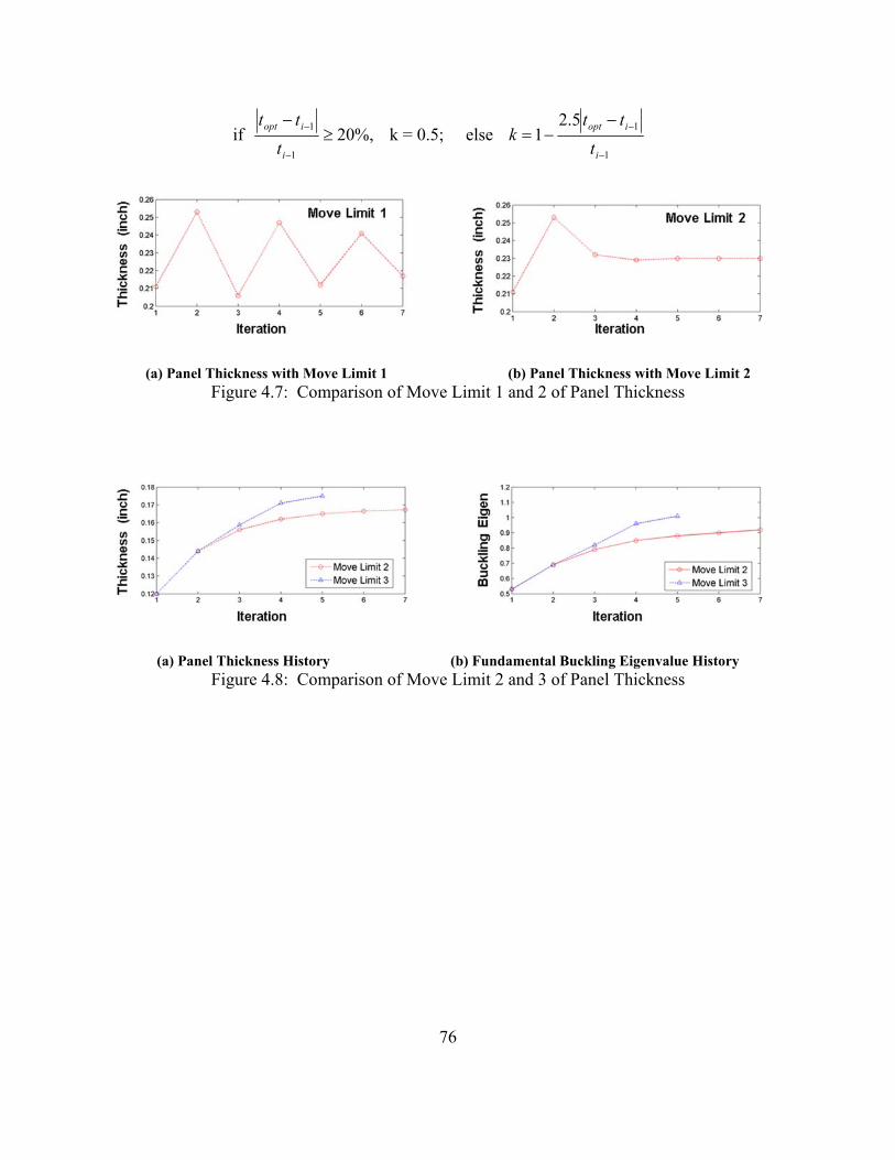
76

if %,201

1

i

iopt

t

tt k = 0.5; else

1

15.21

i

iopt

t

ttk

(a) Panel Thickness with Move Limit 1 (b) Panel Thickness with Move Limit 2 Figure 4.7: Comparison of Move Limit 1 and 2 of Panel Thickness

(a) Panel Thickness History (b) Fundamental Buckling Eigenvalue History Figure 4.8: Comparison of Move Limit 2 and 3 of Panel Thickness

77

4.4 Results of Un-Stiffened Panel Optimization

In the local panel optimization, stress and buckling constraints are applied on all the local panels.

The static, buckling and flutter analyses are carried out for the optimal CRM wing so as to check

the multidisciplinary constraints for the global wing. Figure 4.9 is a trace plot for the

convergence history of the un-stiffened panel optimization. The global wing weight, 1st buckling

eigenvalue of global wing, aerodynamic lift force, and the number of panels that violate the

buckling constraint are traced in all the optimization iterations. The results of un-stiffened panel

optimization are summarized in Table 4.2. It shows the optimal CRM design, which is obtained

in the seventh iteration, satisfies the buckling constraints. However, the wing weight increases

66.1% compared to the baseline CRM design.

Table 4.2: Results of Un-Stiffened Panel Optimization

Baseline Design Local Panel Optimized

Structural Weight of CRM Design (lbs) 11,599 19,269

1st Buckling Eigenvalue at AOA -2° 0.467 1.0009

1st Buckling Eigenvalue at AOA 6° 0.141 1.0002

Buckling eigenvalue is the dominant constraint as compared to the stress constraint for most

local panels. Figure 4.10 presents the fundamental buckling eigenvalues of the local panels in the

optimal CRM wing. Most of the buckling eigenvalues have been optimized to 1. Much greater

buckling eigenvalues are observed in some local panels, the reason is that the thicknesses of

those panels have approached 0.05 inch, which is the lower bound of panel thickness.

78

Figure 4.9: Convergence History of Un-Stiffened Panel Optimization of NASA CRM Wing

Figure 4.10: Fundamental Buckling Eigenvalues of Optimal Local Panels

79

The results in the Figure 4.9 show that the convergence criterion is satisfied in the sixth

optimization iteration. However, the fundamental buckling eigenvalues of the global wing in the

two load cases are around 0.9, which does not satisfy the buckling constraint. The panel

thickness modification process, which is described in Figure 4.4, is performed for the CRM

design obtained in the sixth iteration. The buckling eigenvectors of the first ten modes are

computed in the buckling analysis of the global CRM wing. The thicknesses of the buckled local

panels are modified using the formula shown in Eq. 4.4. An optimal wing design is obtained and

two selected buckling mode shapes of the un-stiffened panel optimized design are presented in

Figure 4.11. The corresponding buckling eigenvalues are 1.0066 and 1.0025 respectively. In the

ideal wing design which is dominated by the buckling constraint, most local panels should

buckle together, which also means most panels buckle in the same buckling mode. The buckling

eigenvalues of the first ten buckling modes of the optimal CRM wing are presented in Table 4.3.

In different global buckling mode shapes, the local buckling is observed in different regions. The

result shows that buckling eigenvalues of the first ten modes are very close to 1. It means the un-

stiffened CRM wing has been well optimized.

The distribution of optimal local panel thicknesses is shown in Figure 4.12. In the optimal

design of CRM wing, the thicknesses of local panels decrease from wing root to wing tip. The

results of von Mises stress distribution and displacement of the CRM wing are shown in Figure

4.13 and Figure 4.14, respectively. The maximum stress is observed in the region near the

junction between the outer wing and the inner wing. The maximum von Mises stress is much

higher than the yield stress of the material Aluminum alloy 2024-T3. The displacement

distribution shows that the unstiffened panel optimal CRM design can satisfy the max

displacement constraints defined in the Chapter 3.

80

(a) Angle of Attack -2 Degrees, Lower Skin (b) Angle of Attack 6 Degrees, Upper Skin

Buckling Eigenvalue 1.0066 Buckling Eigenvalue 1.0025

Figure 4.11: Buckling Mode Shapes of Un-Stiffened Panel Optimization Design

Table 4.3: Buckling Eigenvalues of the First Ten Modes

Mode AOA -2o AOA 6o

1 1.0009 1.0002

2 1.0016 1.0025

3 1.0055 1.0058

4 1.0066 1.0093

5 1.0083 1.0164

6 1.0093 1.0201

7 1.0098 1.0211

8 1.0123 1.0263

9 1.0199 1.0322

10 1.0289 1.0322

81

Figure 4.12: Optimal Thicknesses of Wing Panels

(a) Angle of Attack -2 Degrees, Lower Skin (b) Angle of Attack 6 Degrees, Upper Skin

Figure 4.13: von Mises Stress of Un-Stiffened Panel Optimization Design

82

(a) Angle of Attack -2 Degrees (b) Angle of Attack 6 Degrees

Figure 4.14: Displacement in Z Direction of Un-Stiffened Panel Optimization Design

4.5 Summary

The local panel optimization framework EBF3PanelOpt has been developed and applied to the

NASA CRM wing with un-stiffened panels. The thicknesses of un-stiffened local panels are

optimized subject to the stress and buckling constraints. The boundary condition of panel

buckling analysis is defined using the displacements of the grid points on the panel edges. An

iterative panel optimization framework is developed while considering the interaction between

the global wing model and the local panel model. The local panel optimization procedure has

been applied to the baseline CRM design with 3 spars and 37 ribs provided by NASA, which

does not satisfy the buckling constraint. The CRM has been optimized considering strength,

buckling, and displacement constraints by optimizing the panel thickness. The results show that

the buckling eigenvalue is the critical constraint for most of local panels. The un-stiffened panel

optimization procedure shows its efficiency in minimizing wing weight with stress and buckling

constraints.

83

Chapter 5

EBF3PanelOpt: Stiffened Panel Optimization

Optimization of stiffened panel with straight or curvilinear stiffeners has been implemented in

the EBF3PanelOpt framework. Stiffeners are added on the panels to increase the rigidity and

improve the buckling performance of local panels. The stiffened panel optimization is integrated

in the EBF3PanelOpt framework, and has been applied to the optimization of NASA CRM wing

considering stress and buckling constraints. The integration of global wing optimization and

local panel optimization is discussed in this chapter. An approximate method has been developed

for the stiffened panel optimization, in order to optimize both the global wing and local panel

design variables at an acceptable computational cost. An efficient method for optimizing the

curvilinear stiffeners is also presented in this Chapter.

84

5.1 Description of Stiffened Panel

The results of un-stiffened panel optimization show that buckling constraints are critical

constraints for most of local panels. Therefore, there is potential to reduce the panel thickness as

improving the buckling performance of panels using stiffeners. In the stiffened panel

optimization, the local panels are extracted from the finite element model of the global wing

structure. As shown in Figure 5.1, the blade stiffeners, which are modeled using shell elements,

are added on the panels along the spanwise direction to resist the in-plane compression in the

CRM wing skins. The geometry parameterization of stiffeners has been discussed in Chapter 2.

The geometry of each stiffener is defined by 4 shape design variables that define the location and

curvature, and 2 size design variables that define the height and thickness of the stiffener. The

stiffened panel is meshed using a fine grid instead of the coarse grid used in the global model.

The finite element model of panel and stiffeners is created using shell elements.

Figure 5.1: CRM Wing with Stiffened Panels

85

5.2 Interconnection between Global Wing and Stiffened Panel

In the stiffened panel optimization, the panel geometry is changed by adding the stiffeners on the

panels, and panel thickness is also optimized. Then the global wing model needs to be updated

using those optimized shape and size parameters of stiffened panels. The geometry of global

model is rebuilt in two steps using finite element models of local panels: firstly, create panel

surfaces using the local panel FE models; then create stiffener surfaces on the local panel using

the optimal design variables obtained from stiffened panel optimization.

In the local panel analysis, the boundary conditions of local panels are defined using the

displacements on the panel edges. Since the grid nodes of the stiffened panel model do not match

the grids in the global model, the displacements on the panel edges need to be calculated by

interpolation. Figure 5.2 illustrates the translational displacements that are applied on the panel

edges as boundary conditions for the static and buckling analyses. The translational

displacements are computed by interpolating the displacements of the coarse grid extracted from

the global wing model onto the finer grid in the stiffened panel model.

Figure 5.2: Boundary Condition of Stiffened Panel

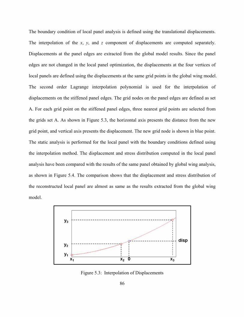
86

The boundary condition of local panel analysis is defined using the translational displacements.

The interpolation of the x, y, and z component of displacements are computed separately.

Displacements at the panel edges are extracted from the global model results. Since the panel

edges are not changed in the local panel optimization, the displacements at the four vertices of

local panels are defined using the displacements at the same grid points in the global wing model.

The second order Lagrange interpolation polynomial is used for the interpolation of

displacements on the stiffened panel edges. The grid nodes on the panel edges are defined as set

A. For each grid point on the stiffened panel edges, three nearest grid points are selected from

the grids set A. As shown in Figure 5.3, the horizontal axis presents the distance from the new

grid point, and vertical axis presents the displacement. The new grid node is shown in blue point.

The static analysis is performed for the local panel with the boundary conditions defined using

the interpolation method. The displacement and stress distribution computed in the local panel

analysis have been compared with the results of the same panel obtained by global wing analysis,

as shown in Figure 5.4. The comparison shows that the displacement and stress distribution of

the reconstructed local panel are almost as same as the results extracted from the global wing

model.

Figure 5.3: Interpolation of Displacements

87

(a) Interpolation Results (b) Results of Global Wing Analysis Figure 5.4: Comparison of Stress Distribution

88

5.3 Panel Thickness Optimization of Stiffened Panel

In the stiffened panel optimization, each local panel has a uniform thickness, which is optimized

considering buckling and stress constraints. Several different types of stiffeners, such as blade, T

shape and L shape stiffener, have been implemented in the EBF3PanelOpt. In the case that the

buckling eigenvalue is the critical constraint, the objective of stiffened panel optimization is to

find the minimum plate thickness that leads the buckling eigenvalue to be greater than 1. As we

have discussed in Chapter 1, the analytic solution of critical buckling stress of stiffened panel

with a thin plate is shown in following formula.

2

CR p=

skin

skin

b

t (5.1)

where tskin is the thickness of panel skin, and bskin is the spacing between two adjacent stiffeners,

p is a constant related to the panel dimension and material properties. This formula is only valid

in the thin plate condition, which means that the plate is very thin relative to the size of the

stiffeners. In that case, the buckling mode is constrained in the small region between the two

adjacent stiffeners, as shown in case (a) of Figure 5.5. If the plate is very thin, the formulas in Eq.

4.8 can be used in the panel thickness optimization.

The effect of plate thickness on the buckling behavior of stiffened panels has been studied. The

fundamental buckling mode shapes and eigenvalues of the stiffened panel with different panel

thicknesses are shown in Figure 5.5 and Figure 5.6. The panel geometry and boundary conditions

are the same in the buckling analyses, in other words the only difference is the plate thickness.

As shown in Figure 5.5, the plate thickness increases from 0.15 inch to 1.0 inch, meanwhile the

wavelength of the 1st buckling mode shape also increases from the spacing between two

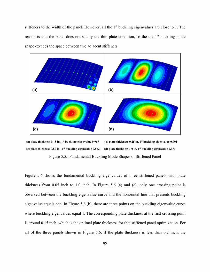
89

stiffeners to the width of the panel. However, all the 1st buckling eigenvalues are close to 1. The

reason is that the panel does not satisfy the thin plate condition, so the the 1st buckling mode

shape exceeds the space between two adjacent stiffeners.

(a) plate thickness 0.15 in, 1st buckling eigenvalue 0.967 (b) plate thickness 0.25 in, 1st buckling eigenvalue 0.991

(c) plate thickness 0.50 in, 1st buckling eigenvalue 0.892 (d) plate thickness 1.0 in, 1st buckling eigenvalue 0.973

Figure 5.5: Fundamental Buckling Mode Shapes of Stiffened Panel

Figure 5.6 shows the fundamental buckling eigenvalues of three stiffened panels with plate

thickness from 0.05 inch to 1.0 inch. In Figure 5.6 (a) and (c), only one crossing point is

observed between the buckling eigenvalue curve and the horizontal line that presents buckling

eigenvalue equals one. In Figure 5.6 (b), there are three points on the buckling eigenvalue curve

where buckling eigenvalues equal 1. The corresponding plate thickness at the first crossing point

is around 0.15 inch, which is the optimal plate thickness for that stiffened panel optimization. For

all of the three panels shown in Figure 5.6, if the plate thickness is less than 0.2 inch, the

90

fundamental buckling eigenvalue is approximately proportional to the square of plate thickness.

That means the thin plate condition is valid in that thin plate region, and the buckling mode

shape is localized in the small pocket between stiffeners. In Figure 5.6 (c), the buckling

eigenvalues in the thin plate region are much smaller than one. Therefore, in order to optimize

that stiffened panel, the stiffener size, such as stiffener height and thickness, should be increased

so as to constrain the buckling in the local pockets between adjacent stiffeners. In the stiffened

panel optimization procedure, a small value is selected as the initial trial plate thickness, then the

buckling analysis is carried out and the panel thickness optimization method discussed in

Chapter 4 is used to search for the optimal panel thickness subject to stress and buckling

constraints.

Figure 5.6: Fundamental Buckling Eigenvalues of Stiffened Panel

91

Figure 5.7 illustrates the searching process of the optimal thickness of stiffened panel. Firstly, a

small value is selected as the trial panel thickness to satisfy the thin plate requirement. For

instance, 0.1 inch is selected as the initial panel thickness in this optimization process. Then the

fundamental buckling eigenvalue is carried out for the stiffened panel with the corresponding

boundary conditions. If the 1st buckling eigenvalue satisfies the constraint, the searching process

is stopped and output the optimal panel thickness. If the buckling eigenvalue does not satisfy that

criterion, the panel thickness is optimized and the new buckling eigenvalue is computed again. A

move limit is applied to the panel thickness as the discussion about panel thickness optimization

in Chapter 4. That stiffened panel thickness optimization process has been implemented and

integrated into EBF3PanelOpt.

Figure 5.7: Process of Stiffened Panel Thickness Optimization

5.4 Effect of Stiffener Size in the Stiffened Panel Optimization

We know that the stiffeners can improve the buckling performance of stiffened panel by

restraining the local buckling mode in the small pockets between adjacent stiffeners. As shown

in Figure 5.8 (a), the panel is stiffened by evenly distributed stiffeners with a height of 3 inch and

a thickness of 0.3 inch. The panel thickness is optimized to be 0.24 inch. The corresponding

fundamental buckling eigenvalue of the stiffened panel is 1.01, which is calculated with a

boundary condition applied to the panel edges. Then reducing the stiffener height to 2 inch, we

92

performed the buckling analysis for the same panel. The fundamental buckling eigenvalue

becomes 0.67 and the buckling mode shape is presented in Figure 5.8 (b). The comparison shows

that the stiffener size has significant effect on the buckling performance of the stiffened panel. In

the stiffened panel optimization, proper stiffener height and thickness need to be found at an

acceptable computational cost.

Figure 5.8: Buckling Mode Shapes of Stiffened Panels with Different Stiffener Height

5.5 Number of Stiffeners

The number of stiffeners on the stiffened panel is an important factor for the buckling behavior

of the panel. As has been discussed in Chapter 1, for a thin plate, the critical buckling stress is

related to the ratio of plate thickness and the spacing between two adjacent stiffeners. That

means the buckling performance of stiffened panel can be improved by adding more stiffeners.

However, the total weight of stiffened panel may increase because of the increased weight of

stiffeners.

A study of a stiffened panel is performed to find the best number of stiffeners to minimize the

panel weight subject to stress and buckling constraints. As shown in Figure 5.9, the parallel

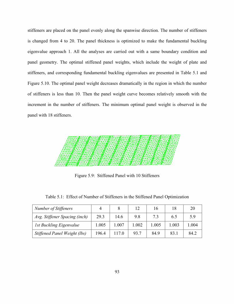
93

stiffeners are placed on the panel evenly along the spanwise direction. The number of stiffeners

is changed from 4 to 20. The panel thickness is optimized to make the fundamental buckling

eigenvalue approach 1. All the analyses are carried out with a same boundary condition and

panel geometry. The optimal stiffened panel weights, which include the weight of plate and

stiffeners, and corresponding fundamental buckling eigenvalues are presented in Table 5.1 and

Figure 5.10. The optimal panel weight decreases dramatically in the region in which the number

of stiffeners is less than 10. Then the panel weight curve becomes relatively smooth with the

increment in the number of stiffeners. The minimum optimal panel weight is observed in the

panel with 18 stiffeners.

Figure 5.9: Stiffened Panel with 10 Stiffeners

Table 5.1: Effect of Number of Stiffeners in the Stiffened Panel Optimization

Number of Stiffeners 4 8 12 16 18 20

Avg. Stiffener Spacing (inch) 29.3 14.6 9.8 7.3 6.5 5.9

1st Buckling Eigenvalue 1.005 1.007 1.002 1.005 1.003 1.004

Stiffened Panel Weight (lbs) 196.4 117.0 93.7 84.9 83.1 84.2

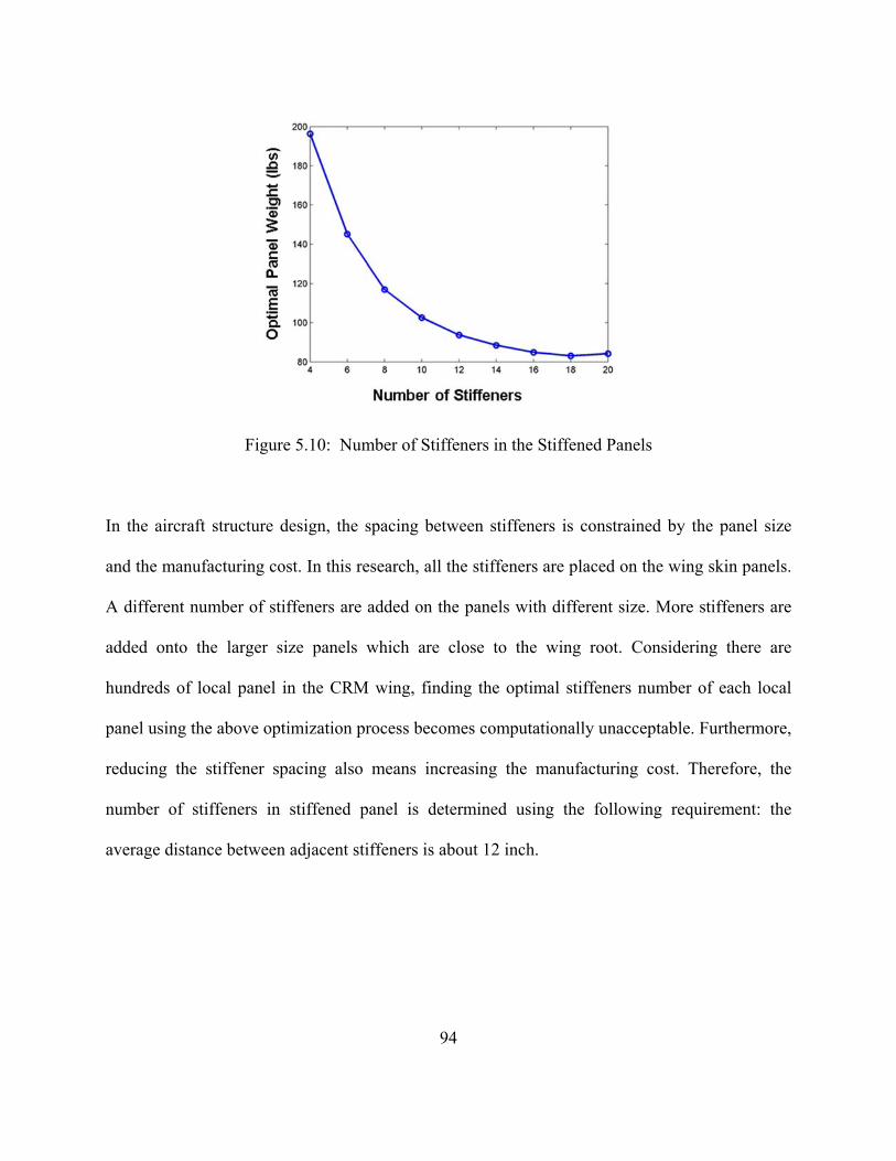
94

Figure 5.10: Number of Stiffeners in the Stiffened Panels

In the aircraft structure design, the spacing between stiffeners is constrained by the panel size

and the manufacturing cost. In this research, all the stiffeners are placed on the wing skin panels.

A different number of stiffeners are added on the panels with different size. More stiffeners are

added onto the larger size panels which are close to the wing root. Considering there are

hundreds of local panel in the CRM wing, finding the optimal stiffeners number of each local

panel using the above optimization process becomes computationally unacceptable. Furthermore,

reducing the stiffener spacing also means increasing the manufacturing cost. Therefore, the

number of stiffeners in stiffened panel is determined using the following requirement: the

average distance between adjacent stiffeners is about 12 inch.

95

5.6 Stiffened Panel Optimization Procedure

The global-local stiffened panel optimization has been performed for the CRM wing with 37

straight ribs, the wing has been presented in the un-stiffened panel optimization of Chapter 4.

Similar as the un-stiffened panel optimization, the stiffened panel optimization process consists

of global wing analysis, which calculates the aerodynamic loads and displacements of the global

CRM wing model, and the stiffened panel analysis, that carries out the static and buckling

analyses for each stiffened panel. The finite element model of stiffened CRM wing is constructed

using shell elements to present the wing panels and stiffeners. Blade stiffeners are added on the

wing skin panels to increase the axial stiffness and improve the buckling performance. In the

global wing analysis, the grid points at the wing root are fixed. Then as similar as the unstiffened

panel optimization, a global static and buckling analysis is carried out to check the stress and

buckling constraints, and generate the global displacement fields for the next iteration of the

stiffened panel optimization. In this research, the stiffened panel thickness is optimized to

minimize the stiffened panel weight using the similar approach of panel thickness optimization

that was discussed in Chapter 4. In each optimization cycle, the global CRM model is updated

using the optimal design variables obtained in local panel optimization. The boundary conditions

of stiffened panels are also updated in each optimization cycle. A minimum thickness

requirement of 0.05 inch is applied to all the local panels. As shown in Eq. 5.2, the convergence

criterion is defined using the number of panels that violate the stress or buckling constraint, and

the relative change of total wing weight in the optimization cycle.

Number of Panels Violate Constraint < 3

%2.01

i

ii

w

ww (5.2)

96

The thickness and height of the stiffeners in each panel are uniform. In order to find the proper

stiffener size without increasing too much computational time, only six stiffener height and

thickness combinations are considered in the stiffened panel optimization: (2, 0.1), (2, 0.2), (3,

0.2), (3, 0.3), (4, 0.3), (4, 0.4); the first and second values are the stiffener height and thickness in

inch, respectively. The proper stiffener size can be selected by the process illustrated in Figure

5.11. The initial stiffener height is given by the initial panel thickness. Then the panel thickness

optimization is carried out as the iterative optimization process discussed in Figure 5.7. If the

final fundamental buckling eigenvalue does not satisfy the buckling constraint, a higher or

thicker stiffener size combination will be selected to substitute for the previous values.

Figure 5.11: Optimization Process of Stiffener Size

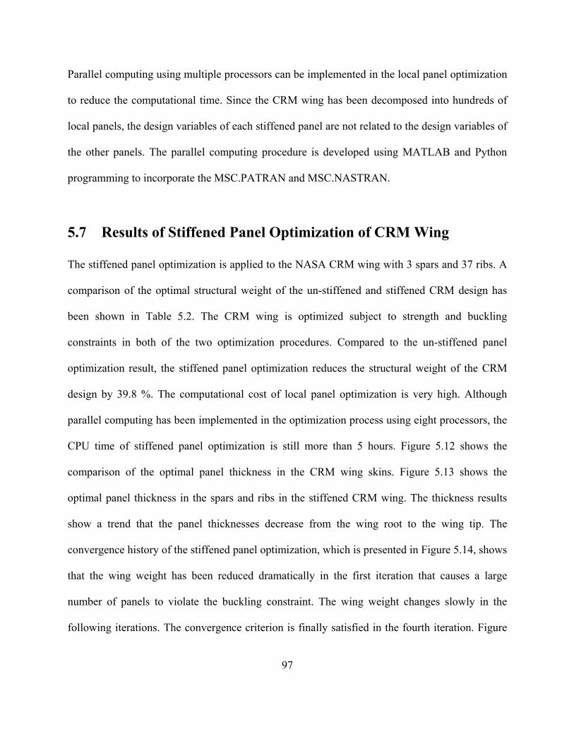
97

Parallel computing using multiple processors can be implemented in the local panel optimization

to reduce the computational time. Since the CRM wing has been decomposed into hundreds of

local panels, the design variables of each stiffened panel are not related to the design variables of

the other panels. The parallel computing procedure is developed using MATLAB and Python

programming to incorporate the MSC.PATRAN and MSC.NASTRAN.

5.7 Results of Stiffened Panel Optimization of CRM Wing

The stiffened panel optimization is applied to the NASA CRM wing with 3 spars and 37 ribs. A

comparison of the optimal structural weight of the un-stiffened and stiffened CRM design has

been shown in Table 5.2. The CRM wing is optimized subject to strength and buckling

constraints in both of the two optimization procedures. Compared to the un-stiffened panel

optimization result, the stiffened panel optimization reduces the structural weight of the CRM

design by 39.8 %. The computational cost of local panel optimization is very high. Although

parallel computing has been implemented in the optimization process using eight processors, the

CPU time of stiffened panel optimization is still more than 5 hours. Figure 5.12 shows the

comparison of the optimal panel thickness in the CRM wing skins. Figure 5.13 shows the

optimal panel thickness in the spars and ribs in the stiffened CRM wing. The thickness results

show a trend that the panel thicknesses decrease from the wing root to the wing tip. The

convergence history of the stiffened panel optimization, which is presented in Figure 5.14, shows

that the wing weight has been reduced dramatically in the first iteration that causes a large

number of panels to violate the buckling constraint. The wing weight changes slowly in the

following iterations. The convergence criterion is finally satisfied in the fourth iteration. Figure

98

5.15 shows that only one panel violates the buckling constraint in the design obtained in the

fourth iteration. The minimum thickness constraint is active in about 20 panels, which makes the

corresponding buckling eigenvalues to be greater than 1. The von Mises stress and displacement

distribution are shown in Figure 5.16 and Figure 5.17 respectively. The buckling analysis is

performed for the optimal CRM wing and the fundamental buckling mode shapes are presented

in Figure 5.18.

Table 5.2: Results of Local Panel Optimization

Un-Stiffened Design Stiffened Design

Optimal Weight (lbs) 19,269 11,593 (39.8% saving)

CPU Time (min) 140 340

(a) Thickness Distribution in Un-Stiffened CRM Wing Skins (b) Thickness Distribution in Stiffened CRM Wing Skins

Figure 5.12: Thickness Distribution of Un-Stiffened and Stiffened NASA CRM Wing

99

Figure 5.13: Optimal Thickness of Spars and Ribs of Stiffened NASA CRM Wing

Figure 5.14: Convergence History of Stiffened Panel Optimization of NASA CRM Wing

100

Figure 5.15: Fundamental Buckling Eigenvalues of Optimal Local Panels

(a) Angle of Attack -2 Degrees, Lower Skin (b) Angle of Attack 6 Degrees, Upper Skin

Figure 5.16: von Mises Stress of Stiffened Panel Optimization Design

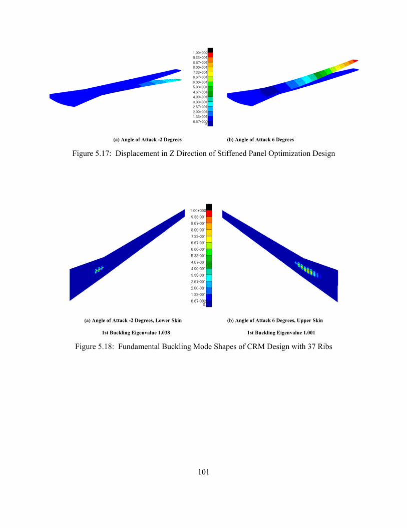
101

(a) Angle of Attack -2 Degrees (b) Angle of Attack 6 Degrees

Figure 5.17: Displacement in Z Direction of Stiffened Panel Optimization Design

(a) Angle of Attack -2 Degrees, Lower Skin (b) Angle of Attack 6 Degrees, Upper Skin

1st Buckling Eigenvalue 1.038 1st Buckling Eigenvalue 1.001

Figure 5.18: Fundamental Buckling Mode Shapes of CRM Design with 37 Ribs

102

5.8 Integration of Global Wing and Local Panel Optimization

5.8.1 Global-Local Optimization Framework

In the local panel optimization, the local panels are optimized by the EBF3PanelOpt and the

global wing model is updated using these optimal parameters of the local panels. However, the

global wing topology, such as the number and shape of spars and ribs, is not optimized by the

EBF3PanelOpt. In order to search the best combination of global wing design variables and

local panel design variables, both global wing optimization and local panel optimization should

be incorporated into an integrated optimization framework. The objective of the optimization is

to minimize the wing weight subject to stress, buckling and flutter constraints. The design

variables in the global-local optimization framework can be decomposed into topology variables

of global wing and local panel design variables. The global wing topology variables include the

design variables which determine the number of spars and ribs (termed numerical variables), and

the design variable which define the shape of spars and ribs (termed shape variables). The local

panel variables are optimized in local panel optimization with a set of fixed global wing design

variables. As illustrated in Figure 5.19, the optimal weight of stiffened wing can be computed

using a set of global variables which define the geometry of spars and ribs. The geometry of

global wing with curvilinear spars and ribs is created using a set of numerical variables and

topology design variables in the EBF3WingOpt. Then in the stiffened panel optimization, the

optimal weight of the wing structure is computed by optimizing the local panel design variables,

such as the panel thickness, height and thickness of stiffeners, and curvature of stiffeners.

103

Figure 5.19: Optimal Weight Calculation of Stiffened CRM Wing

In this research, the integration of global wing optimization and local panel optimization is

implemented using a two-step optimization approach, which is presented in Figure 5.20. In the

first step optimization, the number of the spars and ribs are optimized, and a set of global shape

variables of the spars and ribs are fixed. In this optimization stage, the ribs are distributed evenly

in each wing box. The local panel variables of the aircraft wing are optimized in the stiffened

panel optimization so as to minimize the structural weight. The optimal wing weight is sent to

the optimizer. Then the number of spars and ribs are optimized using particle swarm

optimization (PSO) to find the aircraft wing design with minimum weight. A convergence

criterion is defined for the iterative global-local optimization as the relative change of optimal

wing weight is less than 1% in two consecutive iterations.

104

Figure 5.20: Integrated Global-Local Optimization Framework

In the second optimization step, the shape variables of spars and ribs are optimized with the fixed

numerical variables of spars and ribs, which are obtained in the first step optimization. The shape

variables of spars and ribs are subjected to the constraints in Table 3.7. Similar to that in the first

step, the wing structure with curvilinear spars and ribs, which is constructed using the

EBF3WingOpt module, is optimized using EBF3PanelOpt to output the optimal weight of that

wing design to the optimizer. Compare to the numerical variables of global wing, the wing shape

variables have a much more complex design space, which means the computational cost of shape

optimization of spars and ribs is much higher. The parallel computing has been implemented for

105

the local panel optimization using MATLAB to reduce the CPU time. An optimal wing design

with straight stiffeners can be obtained through the first and second step optimization. Then the

stiffened panels are optimized using curvilinear stiffeners to improve the buckling performance

and minimizing the structural weight.

5.8.2 Approximate Stiffened Panel Optimization

The integration between global wing optimization and local panel optimization is

computationally expensive. A more efficient panel optimization approach needs to be developed

to reduce the computational cost. In the global-local optimization, the objective of stiffened

panel optimization is to find the optimal weight of the CRM design with fixed wing internal

topology. We are concerned about the optimal wing weight rather than the details of the stiffened

CRM wing, an approximate method can be used to find the approximate optimal wing weight

with a much less computational cost, compared to the stiffened panel optimization discussed

earlier in this chapter. In the previous thickness distribution results obtained by local panel

optimization, the panel thickness decreases from the wing root to the wing tip. This trend means

that the thickness of a certain panel can be guessed using the thicknesses of its nearby panels. In

other words, we do not need to run the static and buckling analyses for all the hundreds of local

panels in the CRM wing to optimize the thicknesses of the local panels. In this case, the

computational cost of stiffened panel optimization can be reduced dramatically. In this research,

an approximate method is developed so as to find the approximate stiffened panel design

variables in a more efficient way. In each optimization cycle of the local panel optimization, only

20% ~ 25% selected panels are optimized by the stiffened panel analysis. The approximate

106

thicknesses of other panels can be obtained using a third order polynomial curve that fits to those

optimized panel thicknesses.

Figure 5.21: Upper Skin Panels

The approximate optimization approach has been applied to optimize the thickness of the upper

skin panels in the CRM wing with 3 spars and 37 ribs. As shown in Figure 5.21, the upper skin

panels are divided into two groups: panels No. 1 to 37 in ‘Group 1’ are close to the trailing edge,

and panels No. 38 to 74 in ‘Group 2’ are close to the leading edge. Five evenly distributed panels

are selected in each panel group and optimized by stiffened panel analysis. Then a third order

polynomial curve is created by fitting to the five panel thicknesses in each group. The

thicknesses of other panels are computed using the third order polynomial. The comparison of

the actually optimized panel thickness and approximately optimized thickness calculated by the

polynomial curve fitting are shown in Figure 5.22. Compared to the results of stiffened panel

optimization, the errors of total weight of the two panel groups obtained using the approximate

approach are 1.2% and -2.3% respectively.

107

(a) Upper Skin Group 1, Error of Weight 1.2% (b) Upper Skin Group 2, Error of Weight -2.3%

Figure 5.22: Comparison of Optimal Thickness of Upper Skin Panels

Figure 5.23: Decomposition of CRM Wing Panels

In the approximate stiffened panel optimization approach, the panels of the CRM wing with 3

spars are decomposed into 9 groups as shown in Figure 5.23. The panels in each group locate

along the spanwise direction. The approximate panel optimization and the previous stiffened

panel optimization are carried out for each group of panels. The error of the approximate optimal

weight has been calculated and shown in Table 5.3. All the optimal weight errors of the panel

108

groups are less than 3%. Table 5.4 shows the computation time of the approximate optimization

is only 135 minutes compared to 340 minutes using the stiffened panel optimization. Parallel

computing are performed using eight processors in the two optimization cases. The error of

approximate optimal weight of the CRM wing is about 0.7%.

Table 5.3: Error of Approximate Stiffened Panel Optimization of Panel Groups

Panel Group 1 2 3 4 5 6 7 8 9

Approx. Optimal Weight(lb) 1585 2587 1181 1856 727 1922 305 942 408

Optimal Weight (lb) 1622 2556 1205 1885 738 1917 310 945 416

Relative Error(%) -2.3 1.2 -2.0 -1.5 -1.5 0.3 -1.6 -0.3 -0.2

Table 5.4: Comparison of Computation Time

Stiffened Panel Optimization Approximate Panel Optimization

Optimal Weight(lb) 11,593 11,514

CPU Time(min) 340 135

The approximate stiffened panel optimization has been applied to several CRM wing designs to

evaluate the errors of wing weight. Based on the results, the distribution of the weight errors of

panel groups can be considered as a random distribution between -3% and 3%. Since there are 9

groups in a CRM wing with 3 spars, the error of the total weight of CRM can be estimated using

Eq. (5.3).

(5.3)

where % %, is the weight of the ith group of panels. The cumulative probability

distribution of the wing weight error of approximate panel optimization is calculated using the

error ∑ / ∑

109

Equation 5.8. As presented in Figure 5.24, the error of the optimal weight of the CRM wing is

less than 1.04% with 90% confidence. This error of optimal wing weight is acceptable in the

global-local stiffened panel optimization.

Figure 5.24: Cumulative Probability Distribution of Weight Error

5.8.3 Initial Panel Thickness

Initial panel thicknesses should be defined in the local panel optimization. The computational

cost of the iterative optimization procedure can be saved by choosing proper panel thicknesses.

In the approximate panel optimization of stiffened CRM wing, initial panel thicknesses are

computed using the interpolation of panel thicknesses. The panel thickness interpolation is

illustrated in Figure 5.25. The CRM wing with 3 spars and 37 ribs has been optimized in

stiffened panel optimization and the optimal panel thicknesses are known. A new CRM design

with 20 ribs is created using given global wing design variables. The coordinates of the panel

110

centroids in the two CRM wings are calculated. A third order polynomial curve is created by

fitting to the optimized panel thicknesses and corresponding Y-coordinates of panel centroids of

the CRM wing with 37 ribs. Then the initial panel thickness in the CRM wing with 20 ribs can

be calculated using the corresponding Y-coordinates of panel centroids and the fitted polynomial.

Figure 5.25: Initial Panel Thickness Calculation of Stiffened Panel Design

5.8.4 Results of Integrated Global-Local Optimization

The integrated global-local optimization is performed for the CRM wing. In this optimization

case, the three spars of the CRM wing are fixed. Considering the relatively poor bucking

performance of large size local panels, the number of ribs in inner wing and outer wing are given

independently and subject to the following constraints:

6 ≤ Number of Ribs in Inner Wing ≤ 12

10 ≤ Number of Ribs in Outer Wing ≤ 30 (5.4)

The finite element model of CRM designs are created in global wing module EBF3WingOpt

using the global wing design variables, and are optimized by the approximate stiffened panel

optimization to evaluate the optimal weight of the CRM wing. As presented in Figure 5.20, the

integrated global-local optimization is organized using a two-step approach. The first step of the

111

global-local optimization procedure is performed for the CRM wing with three spars. The

number of ribs in each wing box is optimized using particle swarm method. Five design particles

are created and analyzed in each optimization cycle. A converged optimal design is obtained in

the fifth iteration. The minimum wing weight obtained in each iteration is presented in Figure

5.26.

Figure 5.26: Convergence History of Optimal Wing Weight

The optimal wing weights of the 25 CRM designs optimized by the approximate stiffened panel

optimization are shown in Figure 5.27. The CRM wing with less than 20 or more than 40 ribs are

much heavier than the optimal design. The reason is a wing structure with too less ribs also has

large size skin panels, which is usually relatively poor in buckling resistance. That means the

thicknesses of those large size panels have to be increased to resist the panel buckling.

The minimum wing weight 11,307 lb is observed in the CRM wing with 9 inner wing ribs and 17

outer wing ribs. The details of the optimal CRM wing, including the local panels and stiffeners,

are shown in Figure 5.28. Different numbers of blade stiffeners are placed on the wing skin

panels along the spanwise direction. Figure 5.29 presents the optimal panel thicknesses of the

wing skins, spars and ribs. The thicknesses of the panels close to wing tip have approached the

112

lower bound of 0.05 inch. The mid-spar panel that is close to the wing root has the highest

thickness which of 0.43 inch.

Figure 5.27: Approximate Optimal Weight of CRM Wing with Stiffened Panels

Figure 5.28: Geometry of CRM Wing with 9 Inner Wing Ribs and 17 Outer Wing Ribs

Figure 5.29: Thickness Distribution of Optimal CRM Design

113

The buckling and flutter analyses are performed for the optimal CRM design to check the

buckling and dynamic flutter constraints. The static aeroelastic stress is evaluated using

Kreisselmeier- Steinhauser (KS) criteria [85]. The dynamic pressure of the onset of flutter is also

calculated and presented in Table 5.5. The optimal CRM wing satisfies all the constraints.

Because of the complex design space of shape variables, the computational cost of the second

step optimization, which optimizes the shape variables of spars and ribs, is very expensive.

Currently, the second step optimization of the global-local framework is not performed for the

CRM wing. Parallel computing has been implemented in the stiffened panel optimization using

MATLAB programming. The drawback of the MATLAB parallel computing is only 12

processors can work simultaneously. In future, the parallel computing will be developed in

Python environment to improve the computational efficiency.

Table 5.5: Constraints of Optimal CRM Design

Constraints Optimal Design Low Bound Up Bound

M0.85 AOA -2 Degree KS 0.253 NA 1

M0.85 AOA 6 Degree KS 0.842 NA 1

1st Buckling Eigenvalue AOA -2 Degree 1.041 1.0 NA

1st Buckling Eigenvalue AOA 6 Degree 1.027 1.0 NA

Flutter Dynamic Pressure (psi) 9.68 2.1 NA

114

5.9 Optimization of Panel with Curvilinear Stiffeners

In the stiffened panel optimization described previously, the quasi-straight stiffeners are evenly

distributed on the wing panels. In order words, the shape of stiffeners is not optimized in the

optimization process. Most of the previous research studies about the stiffener topology

optimization focus on a single stiffened panel and typical load cases, such as uniform

compressive, tensile or shear loads, as shown in Figure 5.30. For the local panels in the CRM

wing, the actual loads applied on the panel edges are non-uniform and more complicated.

Computationally expensive evolution algorithms, such as genetic algorithm and particle swarm

optimization, are widely used in the shape optimization of stiffeners. The common situation is

that thousands of stiffened panel analyses are required to find the optimal design of the single

stiffened panel. Considering there are hundreds wing panels in the CRM wing, an efficient

optimization tool is needed to optimize the panel with curvilinear stiffeners at an acceptable

computational cost.

Figure 5.30: Typical Load Cases of Panels

115

In this section, the wing panels are optimized using curvilinear stiffeners to improve the buckling

performance and minimize panel weight. The curvilinear stiffeners are parameterized using

Linked Shape Method so as to reduce the number of design variables. As illustrated in Figure

5.31, three parameters are used to define a set of curvilinear stiffeners on a wing panel. The

locations of starting points are determined by the ratio of the two spacing Space_1_s and

Spar_9_s. The control point line is the mid-line between the top edge and the bottom edge of that

panel. The control points are determined by the ratio of Space_1_c and Spar_9_c. The locations

of ending points are computed using the end points ratio. As shown in Table 5.6, only five design

variables are required to define the curvilinear stiffeners on one panel. The height and thickness

of the stiffeners are uniform.

Table 5.6: Design Variables in Curvilinear Stiffener Optimization

DV1 Stiffener Height

DV2 Stiffener Thickness

DV3 Start Points Ratio

DV4 Control Points Ratio

DV5 End Points Ratio

Figure 5.31: Geometry Parameterization of Curvilinear Stiffeners

116

The optimization procedure for the curvilinear stiffener optimization is presented in Figure 5.32.

Two flight conditions are considered for the CRM wing: angle of attack is -2 degrees or 6

degrees. The shape design variables of curvilinear stiffeners are generated for creating the

geometry of stiffened panel. The size design variables of curvilinear stiffeners are created to

define the height and thickness of stiffeners. The panel thickness is optimized using the panel

thickness optimization process described earlier in this chapter. The response values, such as

panel weight, fundamental buckling eigenvalue, maximum von Mises stress are sent to the

optimizer for generating the new design variables for the next optimization cycle. The curvilinear

stiffened panel optimization is implemented using two optimization schemes: particle swarm

optimization, and a two-step gradient optimization method. The particle swarm optimization is

carried out with 20 particles. The convergence history of the first 200 iterations is shown in

Figure 5.33. The optimal weight of the stiffened panel is 157.4 lbs, which is much heavier than

the initial stiffened panel with evenly distributed quasi-straight stiffeners.

Figure 5.32: Optimization Procedure of Curvilinear Stiffeners

117

Figure 5.33: History of Curvilinear Stiffeners Optimization Using PSO

The stiffened panel is also optimized using a two-step method based on the initial design. In the

first step, the spacing between those stiffeners is optimized using gradient method to minimize

the panel weight subject to the stress and buckling constraints. The stiffener shape is not

optimized in this step. Then the shape variables of stiffeners are optimized in the second step to

obtain curvilinear stiffeners, also using gradient optimization method. The optimal panel weight

and computational time are presented in Table 5.7. It shows that the panel weight has been

reduced by the two-step method at about 10% computational cost compared to the PSO method.

Figure 5.34: Curvilinear Stiffener Optimization Using Two-Step Approach

118

Table 5.7: Optimization Results of Curvilinear Stiffened Panel

Initial Design PSO 1st Step Optimum 2nd Step Optimum

Panel Weight (lbs) 105.5 157.4 103.1 101.9

1st Buckling Eigenvalue 1.003 1.005 1.003 1.001

CPU Time(min) 615 37 26

In the optimal stiffened panel, it is observed that the stiffeners are not very curved. Some

stiffened panels obtain by PSO method have very curved stiffeners but much poorer buckling

performance. As we know, the optimal placement of stiffeners depends on the stress distribution

in the panel. In order to study this problem, a static analysis is carried out for an example local

panel with spanwise stiffeners. As shown in Figure 5.35, the X and Y stress components of the

stiffened panel are compressive, in which case the stress in the Y component is dominant. The Y

component dominant compressive stress distribution is also observed in most of other wing skin

panels. This phenomenon can explain the optimal curvilinear stiffeners locate along the spanwise

direction.

Figure 5.35: Stress Resultant of an Example Stiffened Panel

119

We have known that the optimal shapes and positions of curvilinear stiffeners depend on the

stress distribution in that stiffened panel. The stress distribution computed in the static analysis is

not used in the previous optimization process. There is potential to improve the efficiency of

stiffener optimization by incorporating the stress distribution in the optimization process. The

analytic solution of critical buckling stress of a rectangular stiffened plate has been described in

the previous chapters, as shown in Eq. 5.5. Therefore, the Eq. 5.6 can be derived to describe the

relation between the spacing between two adjacent stiffeners and the longitudinal compressive

stress in the pocket bordered by the two stiffeners.

(5.5)

/

(5.6)

Figure 5.36: Stiffener Optimization Using Y-Component Stress

120

Figure 5.37: Average Y-Component Stress in Panel Sections

A stiffened panel with five evenly distributed stiffeners, which is extracted from the upper wing

skin, is studied. As shown in Figure 5.36, the Y-component stress resultant distribution of the

stiffened panel is computed using MSC.NASTRAN. The stiffened panel is divided into six

sections by the five stiffeners. The average Y-component stress in each panel section is

calculated and presented in Figure 5.37. It shows that the Y-component compressive stress in the

left side of the panel is much less than the Y-component stress in the right side of the panel.

According to Eq. 5.10, the panel buckling performance can be improved by reducing the stiffener

spacing in the high compressive stress region. Therefore, the stiffener locations are updated using

the spacing calculated by the Eq. 5.11. The right picture in Figure 5.36 shows the Y-component

stress in the new stiffened panel. In that panel design, the spacing_1 is about 70% greater than the

spacing_6. The plate thicknesses of the two stiffened panel are optimized to minimize the panel

weight subject to the stress and buckling constraints. The optimal weight of the initial stiffened

panel with evenly distributed stiffeners is 59.2 lbs. The optimal weight of the panel with non-

uniform spacing is reduced to 53.7 lbs, or 9.3% weight reduction.

In order to compare the efficiency of different optimization schemes, three curvilinear stiffener

optimization methods are compared. In the optimization scheme 1, the stiffeners are optimized

121

using the Eq. 5.11 in the first step. In the second step, the gradient optimization method is used to

optimize the shape and size variables of the curvilinear stiffeners. The fundamental buckling

mode shape of optimal stiffened panel obtained by scheme 1 is shown in Figure 5.38. In the

optimization scheme 2, the stiffeners are optimized using the gradient method to minimize the

panel weight. Particle swarm optimization is used in the optimization scheme 3 to optimize the

shape and size variables of the stiffeners. The boundary conditions are the same in the three

optimization schemes. The three optimization schemes are compared in Table 5.8. The minimum

panel weight is obtained using scheme 1 at a much less computational time than the other two

optimization schemes. It shows the advantage of incorporating the stress information for the

stiffened panels into the optimization of curvilinear stiffeners.

(a) Initial Panel with Evenly Distributed Stiffeners (b) Optimized Panel using Scheme 1

Figure 5.38: Fundamental Buckling Mode Shape of Stiffened Panel

Table 5.8: Comparison of Stiffener Optimization Schemes

Initial Panel Scheme 1 Scheme 2 Scheme 3

Optimal Weight (lbs) 59.2 50.7 51.6 52.4

1st Buckling Eigenvalue 1.002 1.001 1.003 1.002

CPU Time (min) N.A. 23 65 331

122

5.10 Summary

A stiffened panel optimization procedure has been developed and applied to the structural design

of the subsonic NASA CRM wing. Local panel optimization has been carried out for un-

stiffened or stiffened panels to reduce the panel weight considering stress and buckling

constraints. The results of the stiffened panel optimization have shown that the structural weight

can be reduced by about 40%, compared to the results of un-stiffened panel optimization.

The interaction between global wing optimization and local panel optimization is studied to

integrate the EBF3WingOpt and EBF3PanelOpt into a global-local optimization framework.

The computational time of the stiffened panel optimization is reduced about 60% using an

approximate panel optimization technique.

The integrated global-local optimization is implemented using a two-step approach and parallel

computing. The optimization of global wing design variables and local panel design variables are

integrated in the integrated global-local optimization. The minimum wing weight is observed in a

CRM wing with 3 spars, 9 inner wing ribs and 17 outer wing ribs, subject to strength, buckling

and flutter constraints. The optimization of stiffened panel with curvilinear stiffeners is also

studied to exploit the advantage of curvilinear stiffening design. The comparison of three

different optimization schemes shows that the computational time can be significantly saved by

integrating the stress resultants information in the optimization process.

123

Chapter 6

Future Research

In this research, the optimization module EBF3WingOpt has been applied to the Boeing N+2

supersonic aircraft concept and NASA common research model. The fact that the optimal design

has a significant weight reduction and all the constraints are satisfied shows the efficiency of the

multidisciplinary optimization process and the advantage of the use of curvilinear SpaRibs and

non-linear thickness fields. However, some further improvements are still required for the wing

optimization. The aerodynamic loads calculation is implemented using the Doublet-Lattice

method or ZONA51 method, in which the influence of thickness and viscosity is neglected. High

fidelity aerodynamic and aeroelastic solutions can be obtained using CFD analysis. Considering

the large amount of computational time of CFD analysis, it is not recommended to incorporate it

in the computationally expensive optimization process. The CFD analysis can be used to check

the multidisciplinary constraints for the optimal aircraft wing.

In the local panel optimization software package EBF3PanelOpt, the size and shape design

variables, which determine the panel thickness, cross-section and curvature of stiffeners, are

124

optimized in the stiffened panel optimization. At present, all the local panels are perfect without

damages. In future, the damage tolerance of the panels with local damages (crack) will be

integrated in the EBF3PanelOpt.The interaction between local damages and stiffeners will be

studied.

For a complex structural model, such as the Boeing HSCT wing and the NASA CRM wing, the

computational cost of global-local multidisciplinary optimization is very high because of the

large number of design variables and complex finite element model. The integrated global-local

optimization is implemented using a two-step approach and parallel computing. The optimal

number of ribs of the CRM wing is obtained in the first step optimization. The shape

optimization of curvilinear spars and ribs will be carried in the second step optimization based on

the optimal CRM design obtained in the first step optimization. The optimization of curvilinear

stiffeners will be performed based on the optimal CRM wing with curvilinear SpaRibs which is

obtained in the second step optimization.

The complex design space of shape variables forces the computational cost of the second step

optimization to be very high. In this research, the optimization package of EBF3WingOpt and

EBF3PanelOpt is developed using MATLAB and Python programming. Parallel computing can

be implemented using MATLAB programming very easily. However, the maximum number of

processors in the MATLAB parallel computing toolbox currently is mere 12, which limits the

potential efficiency of the application of the global-local optimization. That problem can be

solved by implementing the parallel computing on multi-processor computers using Python

programming. Massively parallel processing architectures Graphics Processing Units (GPU) is

widely used in parallel computing. Improving the computational efficiency using GPU will also

be considered in future work.

125

Bibliography

[1] Schmit, L. A., "Structural Design by Systematic Synthesis", Second Conference on

Electronic Computation, ASCE, Pittsburg, 105-132, 1960.

[2] Schmit, L. A., and Ramanathan, R. K., “Multilevel Approach to Minimum Weight Design

including Buckling Constraints”, AIAA Journal, Vol. 16, No. 2, 1978, pp. 97-104.

[3] Schmit, L. A., “Structural Synthesis: Its Genesis and Development,” AIAA Journal, Vol.

19, No. 10, 1981, pp. 1249–1263.

[4] Haftka, R. T., Starnes, J. H., Jr., Barton, F. W., and Dixon, S. C., “Comparison of Two

Types of Optimization Procedures for Flutter Requirements,” AIAA Journal, Vol. 13, No.

10, 1975, pp. 1333–1339.

[5] Haftka, R. T., “Optimization of Flexible Wing Structures Subject to Strength and Induced

Drag Constraints,” AIAA Journal, Vol. 14, No. 8, 1977, pp. 1106–1977.

[6] Starnes, J. H, and Haftka, R. T., “Preliminary design of composite wings for buckling,

strength, and displacement constraints,” Journal of Aircraft, Vol. 16, No. 8, 1978, pp. 564-

570.

[7] Sobieszczanski-Sobieski, J., “Application of Computer-Aided Aircraft Design in a

Multidisciplinary Environment”, Journal of Aircraft, Vol. 11, No. 7, 1974, pp. 369-370.

126

[8] Miettinen, K., Nonlinear Multiobjective Optimization. Springer. 1999.

[9] Seeger, J. and Wolf, K., “Multi-objective Design of Complex Aircraft Structures Using

Evolutionary Algorithms,” Journal of Aerospace Engineering, October, 2011, vol. 225,

No.10, 1153-1164.

[10] Mastroddi, F. and Gemma, S., “Analysis of Pareto Frontiers for Multidisciplinary Design

Optimization of Aircraft”, Aerospace Science and Technology, Volume 28, Issue 1, July

2013, 40–55.

[11] Marin, L., Trisa, D. and Badallo, P., “Optimization of Composite Stiffened Panels Under

Mechanical and Hygrothermal Loads Using Neural Networks and Genetic Algorithms,”

Composite Structures, 2012, 3321-3326.

[12] Sobieszczanski-Sobieski, J., and Haftka, R. T., “Multidisciplinary Aerospace Design

Optimization: Survey of Recent Developments,” Structural Optimization, Vol. 14, 1997, pp.

1-23.

[13] Rabeau, S., Depince P., Bennis, F., and Janiaut, R., “Comparison of Global and Local

Treatment for Coupling Variables into Multidisciplinary Problems”, 11th AIAA/ISSMO

Multidisciplinary Analysis and Optimization Conference, No. AIAA 2006-7066,

Portsmouth, Virginia, 6 - 8 September 2006.

[14] Martins, J. R. R. A., and Lambe, A. B., “Multidisciplinary Design Optimization: A Survey

of Architectures”, AIAA Journal, Vol. 51, No. 9, 2013, pp. 2049-2075.

[15] Locatelli, D., Mulani, S. B. and Kapania, R. K., “Wing-Box Weight Optimization Using

Curvilinear Spars and Ribs (SpaRibs),” Journal of Aircraft, Vol. 48, No. 5, September-

October 2011, pp. 1671–1684.

127

[16] Liu, S., Hou, Y., Sun, X. and Zhang, Y., “A Two-step Optimization Scheme for Maximum

Stiffness Design of Laminated Plates Based on Lamination Parameters,” Composite

Structures, Vol. 94, June, 2012, pp. 3529-3537.

[17] Sobieszczanski-Sobieski, J., James, B. B., and Dovi, A. R., “Structural Optimization by

Multilevel Decomposition”, AIAA Journal, Vol. 23, No. 11, 1985, pp. 1775–1782.

[18] Sobieszczanski–Sobieski, J., “Optimization by Decomposition: A Step from Hierarchic to

Non- Hierarchic Systems,” NASA Langley Research Center TR-CP-3031, Hampton, VA,

September, 1988.

[19] Ragon, S. A., Gürdal, Z., and Starnes, J. H., “Optimization of Composite Box-Beam

Structures Including the Effects of Subcomponent Interaction”, AIAA/

ASME/ASCE/AHS/ASC 35th SDM Conference, Hilton Head, SC, April 18-20, 1994.

[20] Ciampa, P. D. and Nagel, B., “Global Local Structural Optimization of Transportation

Aircraft Wings,” 51st AIAA/ASME/ASCE/AHS/ASC Structures, Structural Dynamics and

Materials Conference, No. AIAA-2010-3098, Orlando, Florida, 12-15 April 2010.

[21] Castellini, F., Riccardi, A., Lavagna, M., and Buskens, C., “Global and Local

Multidisciplinary Design Optimization of Expendable Launch Vehicles,” 52nd

AIAA/ASME/ASCE/AHS/ASC Structures, Structural Dynamics and Materials Conference,

No. AIAA-2011-1901, Denver, Colorado, 4-7 April 2011.

[22] Haftka, R. T., and Watson, L. T., “Decomposition Theory for Multidisciplinary Design

Optimization Problems with Mixed Integer Quasiseparable Subsystems,” Optimization and

Engineering, Vol. 7, No. 2, 2006, pp. 135–149.

128

[23] Dillinger, J. K. S., Abdalla, M. M., Klimmek, T., and Gurdal, Z., “Stiffness Optimization of

Composite Wings with Aeroelastic Constraints”, Journal of Aircraft, Vol.50, No. 4, 2013,

pp. 1159-1168.

[24] Sobieski, I., and Kroo, I., "Aircraft Design Using Collaborative Optimization,” 34th

Aerospace Sciences Meeting and Exhibit, No. AIAA-96-0715, Jan. 15-18, 1996.

[25] Braun, R., Cage, P., Kroo, I., and Sobieski., I., “Implementation and Performance issues in

Collaborative Optimization,” 6th AIAA/NASA/ISSMO Symposium on Multidisciplinary

Analysis and Optimization, Vol. 1, 1996, pp. 295–305.

[26] Kuhn, H. W., and Tucker, A. W., “Nonlinear programming”. Proceedings of 2nd Berkeley

Symposium. Berkeley: University of California Press, 1951, pp. 481–492.

[27] Schmit, L. A., and Chang, K. J., “Optimum Design Sensitivity Based on Approximation

Concepts and Dual Methods,” International Journal for Numerical Methods in Engineering,

Vol. 20, Issue 1, pp. 39–75, January 1984

[28] Canfield, R. A., "High Quality Approximation of Eigenvalues in Structural Optimization,"

AIAA Journal, Vol. 28, No. 6, 1990, pp.1116-1122.

[29] Renner, G. and Ekárt, A., “Genetic algorithms in computer aided design,” Computer-Aided

Design, Vol. 35, Issue 8, July 2003, pp. 709-726.

[30] Venter, G. and Sobieszczanski-Sobieski, J., “Particle Swarm Optimization,” AIAA Journal,

Vol. 41, No. 8, 2003, pp. 1583–1589.

[31] Singh, G., Viana, F. A. C., Subramaniyan, A. K., Wang, L., DeCesare, D. G., Khan, G.,

and Wiggs, G., “Multimodal Particle Swarm Optimization: Enhancements and

Applications,” 12th AIAA Aviation Technology, Integration, and Operations (ATIO)

129

Conference and 14th AIAA/ISSMO Multidisciplinary Analysis and Optimization

Conference, No. AIAA 2012-5570, 17 - 19 September 2012, Indianapolis, Indiana

[32] Ahuja, V. and Hartfield, R. J., “Optimization of UAV Designs for Aerodynamic

Performance Using Genetic Algorithms,” 51st AIAA/ASME/ASCE/AHS/ASC Structures,

Structural Dynamics and Materials Conference, No. AIAA-2010-2759, Orlando, Florida,

12-15 April 2010.

[33] Venter, G. and Sobieszczanski-Sobieski, J., “Multidisciplinary Optimization of a Transport

Aircraft Wing Using Particle Swarm Optimization,” 9th AIAA/ISSMO Symposium on

Multidisciplinary Analysis and Optimization, No. AIAA-2002-644, Atlanta, Georgia, 4-6

Sep. 2002.

[34] Marin, L., Trisa, D., and Badallo, P., “Optimization of Composite Stiffened Panels Under

Mechanical and Hygrothermal Loads Using Neural Networks and Genetic Algorithms”,

Composite Structures, 2012, 3321-3326.

[35] Zingg, D. W., Nemec, M., and Pulliam, T. H., “A Comparative Evaluation of Genetic and

Gradient-Based Algorithms Applied to Aerodynamic Optimization,” European Journal of

Computational Mechanics, Vol. 17, Nos. 1–2, Jan. 2008, pp. 103–126.

[36] Plevris, V. and Papadrakakis, M., “A Hybrid Particle Swarm—Gradient Algorithm for

Global Structural Optimization,” Computer-Aided Civil and Infrastructure Engineering,

Vol. 26, Issue 1, 48–68, January 2011.

[37] Hajikolaei1, K. H., Safari, A., Wang, G. G., and Lemu, H. G., “Surrogate-assisted Self-

accelerated Particle Swarm Optimization”, 10th AIAA Multidisciplinary Design

Optimization Conference, January 2014, National Harbor, Maryland.

130

[38] Goel, T., Vaidyanathan, R., Haftka, R. T., Shyy, W, Queipo, N. V., and Tucker, K.,

“Response Surface Approximation of Pareto Optimal Front in Multi-objective

Optimization,” Computer Methods in Applied Mechanics and Engineering, Vol. 196,

Issues 4–6, 1 Jan. 2007, pp. 879-893

[39] Sunny, M. R., Mulani, S. B., Sanyal, S., Pant, R. S. and Kapania, R. K., “An Artificial

Neural Network Residual Kriging Based Surrogate Model for Shape and Size Optimization

of a Stiffened Panel,” 54th AIAA/ASME/ASCE/AHS/ASC Structures, Structural Dynamics

and Materials Conference, No. AIAA-2013-1689, Boston, Massachusetts, 8-11 April, 2013.

[40] Box, G. E. P. and Wilson, K.B., “On the Experimental Attainment of Optimum

Conditions”. Journal of the Royal Statistical Society Series B13 (1), pp. 1–45.

[41] Liu, B., Haftka, R. T., and Watson, L. T., “Global-local Structural Optimization Using

Response Surfaces of Local Optimization Margins”, Structural Multidisciplinary

Optimization, Volume 27, 2004, pp. 352–359.

[42] Paiva, R. M., Crawford, C., and Suleman, A., “Robust and Reliability-Based Design

Optimization Framework for Wing Design,” AIAA Journal, Vol. 52, No. 4, pp. 711-724.

[43] Jones, D. R., “A Taxonomy of Global Optimization Methods Based on Response Surfaces,”

Journal of Global Optimization, 21: 345–383, 2001

[44] Chandila, P. K., Agarwal, H., and Renaud, J. E., “An Effcient Strategy for Global

Optimization Using Local Kriging Approximations,” 45th AIAA/ASME/ASCE/AHS/ASC

Structures, Structural Dynamics & Materials Conference, 19 - 22 April 2004, Palm Springs,

California.

131

[45] Shimizu, Y. and Kawamoto, H., “An Implementation of Parallel Computing for

Hierarchical Logistic Network Design Optimization Using PSO,” Computer Aided

Chemical Engineering, Vol. 25, 2008, pp. 605-610.

[46] Mussi, L., Daolio, F., and Cagnoni, S., “Evaluation of Parallel Particle Swarm

Optimization Algorithms within the CUDA™ Architecture,” Information Sciences, Vol.

181, Issue 20, 15 October 2011, pp. 4642-4657.

[47] Lundquist, E. E. and Stowell, E. Z., “Critical Compressive Stress for Flat Rectangular

Plates Supported Along All Edges and Elastically Restrained Against Rotation Along the

Unloaded Edges”, Report 733, National Advisory Committee for Aeronautics.

[48] Timoshenko, S., Theory of Elastic Stability, McGraw-Hill Book Company, 1936.

[49] Vescovini, R. and Bisagni, C., “Buckling Analysis and Optimization of Stiffened

Composite Flat and Curved Panels”, AIAA Journal, Vol. 50, No. 4, April 2012, pp. 904-

915.

[50] Block, D., Card, M., and Mikulas, M., “Buckling of Eccentrically Stiffened Orthotropic

Cylinders”, NASA TN D-2960, Aug. 1965.

[51] Megson, T. H. G., Aircraft Structures for Engineering Students, Arnold, 1999.

[52] Ratzersdorfer, J., “Rectangular Plates with Stiffeners: The Buckling of Simply Supported

Plates under Compressive Stress”, Aircraft Engineering and Aerospace Technology,

Volume 14, Issue 9, 1942, pp. 260-264.

[53] Gerard, G., Introduction to Structural Stability Theory, McGraw-Hill Book Company, New

York, 1962.

132

[54] Mittelstedt, C., “Closed-form Analysis of the Buckling Loads of Uniaxially Loaded Blade

Stringer-stiffened Composite Plates Considering Periodic Boundary Conditions”, Thin-

Walled Structures, Vol. 45, No. 4, April 2007, pp. 371-382.

[55] Coburn, B. H., Wu, Z., and Weaver, P. M., “Local Buckling of Blade Stiffened Variable

Angle Tow Panels,” 55th AIAA/ASMe/ASCE/AHS/SC Structures, Structural Dynamics, and

Materials Conference, 13-17 January 2014, National Harbor, Maryland.

[56] Loos, A. C. and MacRae, J. D., “A Process Simulation Model for the Manufacture of a

Blade-Stiffened Panel by the Resin Film Infusion Process,” Composites Science and

Technology, Vol. 56, Issue 3, 1996, pp. 273–289.

[57] Herencia, J. E., Weaver, P. M., and Friswell, M. I., “Optimization of Long Anisotropic

Laminated Fiber Composite Panels with T-Shaped Stiffeners,” AIAA Journal, Vol. 45, No.

10, 2007, pp. 2497–2509.

[58] Williams, J. and Stein, M., “Buckling Behavior and Structural Efficiency of Open-section

Stiffened Composite Compression Panels," AIAA Journal, Vol. 14, May 1976, pp. 1618-

1626.

[59] Bisagni, C. and Vescovini, R., “Fast Tool for Buckling Analysis and Optimization of

Stiffened Panels,” Journal of Aircraft, Vol. 46, No. 6, 2009, pp. 2041–2053.

[60] Vitali, R., Park, O., Haftka, R. T., and Sankar, B. V., “Structural Optimization of a Hat-

Stiffened Panel Using Response Surfaces,” Journal of Aircraft, Vol. 39, No. 1, 2002.

[61] Bedair, O., “Analysis and Limit State Design of Stiffened Plates and Shells: A World

View,” Applied Mechanics Reviews, Vol. 62, No. 2, 2009, pp. 16.

133

[62] Jaunky, N., Knight, N. F., and Ambur, D. R., “Optimal Design of Grid-Stiffened

Composite Panels Using Global and Local Buckling Analyses,” Journal of Aircraft, Vol.

35, No. 3, 1998, pp. 478–486.

[63] Dang, T. D., Kapania, R. K., Slemp, W. C. H., Bhatia, M. and Gurav, S. P., “Optimization

and Postbuckling Analysis of Curvilinear-Stiffened Panels Under Multiple-Load Cases,”

Journal of Aircraft, Vol. 47, No. 5, September–October 2010, pp. 1656-1671.

[64] Zheng, Y. and Dasb, P. K., “Improved Response Surface Method and its Application to

Stiffened Plate Reliability Analysis,” Engineering Structures, Vol. 22, Issue 5, May 2000,

pp. 544–551.

[65] Walch, D., Tetreault, S. and Dervault, F., “Smeared Stiffeners in Panel for Mesh

Simplification at Conceptual Design Phase”, 54th AIAA/ASME/ASCE/AHS/ASC Structures,

Structural Dynamics and Materials Conference, No. AIAA-2013-1809, Boston,

Massachusetts, 8-11 April 2013.

[66] Locatelli, D., Mulani, S. B., and Kapania, R. K., “A Multidisciplinary Analysis

Optimization Environment for Wings Having SpaRibs”, 53rd AIAA/ASME/ASCE/AHS/ASC

Structures, Structural Dynamics and Materials Conference, Honolulu, Hawaii, 23 - 26

April 2012.

[67] Mulani, S. B., Locatelli, D., and Kapania, R. K., “Algorithm Development for Optimization

of Arbitrary Geometry Panels using Curvilinear Stiffeners," 51st

AIAA/ASME/ASCE/AHS/ASC Structures, Structural Dynamics and Materials Conference,

No. AIAA-2010-2674, Orlando, Florida, 12-15 April 2010.

[68] Nicholas, E. D., "Developments in the Friction-Stir Welding of Metals," ICAA-6: 6th

International Conference on Aluminium Alloys, 1998.

134

[69] Caseiro, J. F., Valente, R.A.F., Andrade-Campos, A. and Yoon, J. W., “On the elasto-

plastic buckling of Integrally Stiffened Panels (ISP) joined by Friction Stir Welding (FSW):

Numerical simulation and optimization algorithms,” International Journal of Mechanical

Sciences, Vol. 76, November 2013, pp. 49–59.

[70] Taminger, K. M. B. and Hafley, R. A., "Electron Beam Freeform Fabrication: A Rapid

Metal Deposition Process", Proceedings of 3rd Annual Automotive Composites Conference,

9-10 Sept. 2003, Troy, MI. Society of Plastics Engineers, 2003.

[71] Locatelli, D., Liu, Q., Tamijani, A. Y., Mulani, S., and Kapania, R. K., “Multidisciplinary

Optimization of Supersonic Wing Structures Using Curvilinear Spars and Ribs (SpaRibs)”,

54th AIAA/ASME/ASCE/AHS/ASC Structures Conference, Boston, Massachusetts, April 8-

11, 2013.

[72] Mulani, S. B., Slemp, W. C. H. and Kapania, R. K., “EBF3PanelOpt: An Optimization

Framework for Curvilinear Blade-Stiffened Panels”, Thin-Walled Structures, Vol. 63, 2013,

pp. 13-26

[73] Mulani, S. B., Locatelli, D. and Kapania, R. K., “Grid-Stiffened Panel Optimization using

Curvilinear Stiffeners”, 52th AIAA/ASME/ASCE/AHS/ASC Structures, Structural Dynamics

and Materials Conference, No. AIAA-2011-1895, Denver, Colorado, 4-7 April 2011.

[74] Bhatia, M. and Kapania, R. K., “Stiffener Effectiveness Approach for Optimal Stiffener

Placement on Curvilinear Stiffened Panel”, 50th AIAA/ASME/ASCE/AHS/ASC Structures,

Structural Dynamics and Materials Conference, No. AIAA-2009-2640, Palm Springs,

California, 4-7 April 2009.

135

[75] Albano, E. and Rodden, W. P., “A Doublet_Lattice Method for Calculating Lift

Distributions on Oscillating Surfaces in Subsonic Flows,” AIAA Journal, Vol. 7, NO. 2,

February 1969, pp. 279-285.

[76] Rodden, W. P., Giesing, J. P., and Kalman, T. P., “Refinement of the Nonplanar Aspects of

the Subsonic Doublet-Lattice Lifting Surface Method,” Journal of Aircraft, Vol. 9, NO. 1,

January 1972, pp. 69-73.

[77] Chen, P. C. and Liu, D. D., “A Harmonic Gradient Method for Unsteady Supersonic Flow

Calculations,” Journal of Aircraft, Vol. 22, No. 15, May 1985, pp. 371-379.

[78] MSC Nastran Version 68, Aeroelastic Analysis User’s Guide, MSC.Software Corporation,

2010.

[79] Strong, D. D., Kolonay, R. M., Huttsell, L. J., and Flick, P. M., “Flutter Analysis of Wing

Configurations Using Pre-Stressed Frequencies and Mode Shapes,” 46th

AIAA/ASME/ASCE/AHS/ASC Structures, Structural Dynamics & Materials Conference, No.

AIAA 2005-2173, Austin, Texas, 18 - 21 April 2005

[80] Locatelli, D., Mulani, S. B., and Kapania, R. K., “Parameterization of Curvilinear Spars

and Ribs (SpaRibs) for Optimium Wing Structural Design,” 53rd

AIAA/ASME/ASCE/AHS/ASC Structures, Structural Dynamics and Materials Conference,

Honolulu, Hawaii, April 23-26 2012.

[81] Schumaker, L. L., Spline Functions: Basic Theory, Cambridge Mathematical Library, 2007.

[82] “N+2 Supersonic Concept Development and System Integration”, Technical Report,

Contract NNL08AA16B, Submitted by Boeing Company, Final Draft, July 2009

[83] Chen, D., Britt, R. T., Roughen, K., and Stuewe, D. “Practical Application of

Multidisciplinary Optimization to Structural Design of Next Generation Supersonic

136

Transport”, 13th AIAA/ISSMO Multidisciplinary Analysis Optimization Conference, 13-15

September 2010, Fort Worth, Texas.

[84] Locatelli, D., Optimization of Supersonic Aircraft Wing-Box Using Curvilinear SpaRibs,

Ph.D. thesis, Virginia Polytechnic Institute and State University, 24061, Blacksburg, VA,

2012.

[85] Kreisselmeier, G. and Steinhauser, R., “Systematic Control Design by Optimizing a Vector

Performance Index,” Proceeding IFAC Symposium on Computer-aided Design of Control

Systems, Zurich, Switzerland; 1979. pp. 113–7.

[86] Vassberg, J., DeHaan, M., Rivers, S., and Wahls, R., “Development of a Common

Research Model for Applied CFD Studies”, AIAA Applied Aerodynamics Conference,

Honolulu, HI, August, 2008.