ec306 labour economics - tammy schirle · • monopoly producers and labour demand ... maximizing...

EC306 Labour Economics

Chapter 5" Labour Demand

1

Objectives • Labour demand in the short run - model, graph,

perfectly competitive market

• Labour demand in the long run - model, graph, scale and substitution effects

• Monopoly producers and labour demand

• Elasticity

• Global competition

2

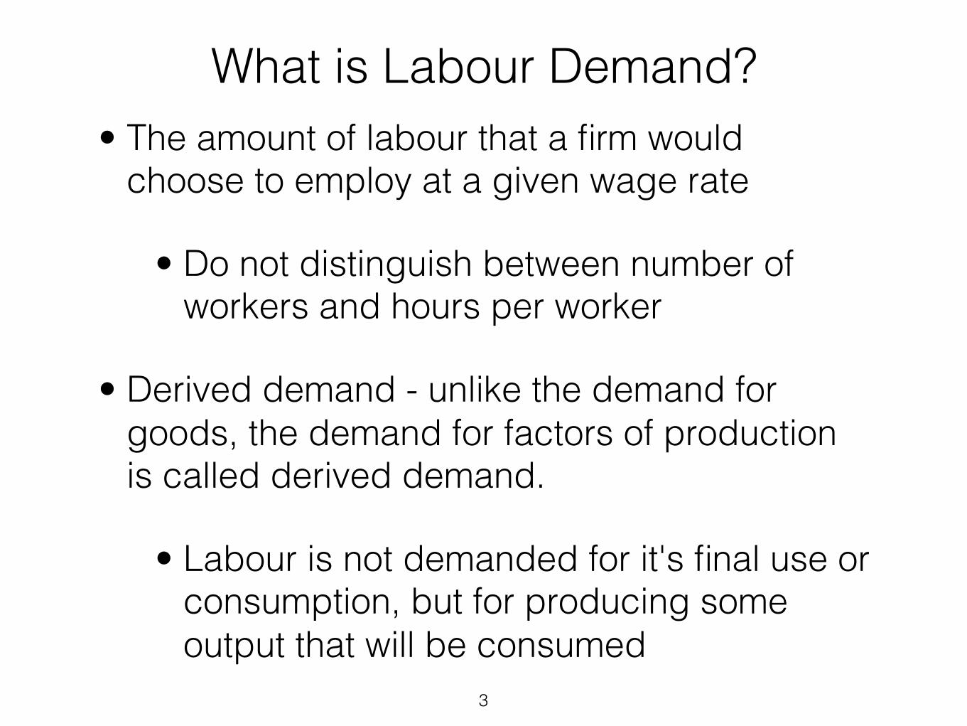
What is Labour Demand? • The amount of labour that a firm would

choose to employ at a given wage rate

• Do not distinguish between number of workers and hours per worker

• Derived demand - unlike the demand for goods, the demand for factors of production is called derived demand.

• Labour is not demanded for it's final use or consumption, but for producing some output that will be consumed

3

Labour demand in the short run

• Short run - period during which one or more factors are fixed ( cannot be adjusted )

• Long run - all factors can be adjusted

• Assume capital K is fixed in the short run

4

• Assume perfect competition in product and labour market

• Large number of firms and workers

• Firms produce homogeneous good

• Workers homogeneous

• Workers and firms are price takers

5


6

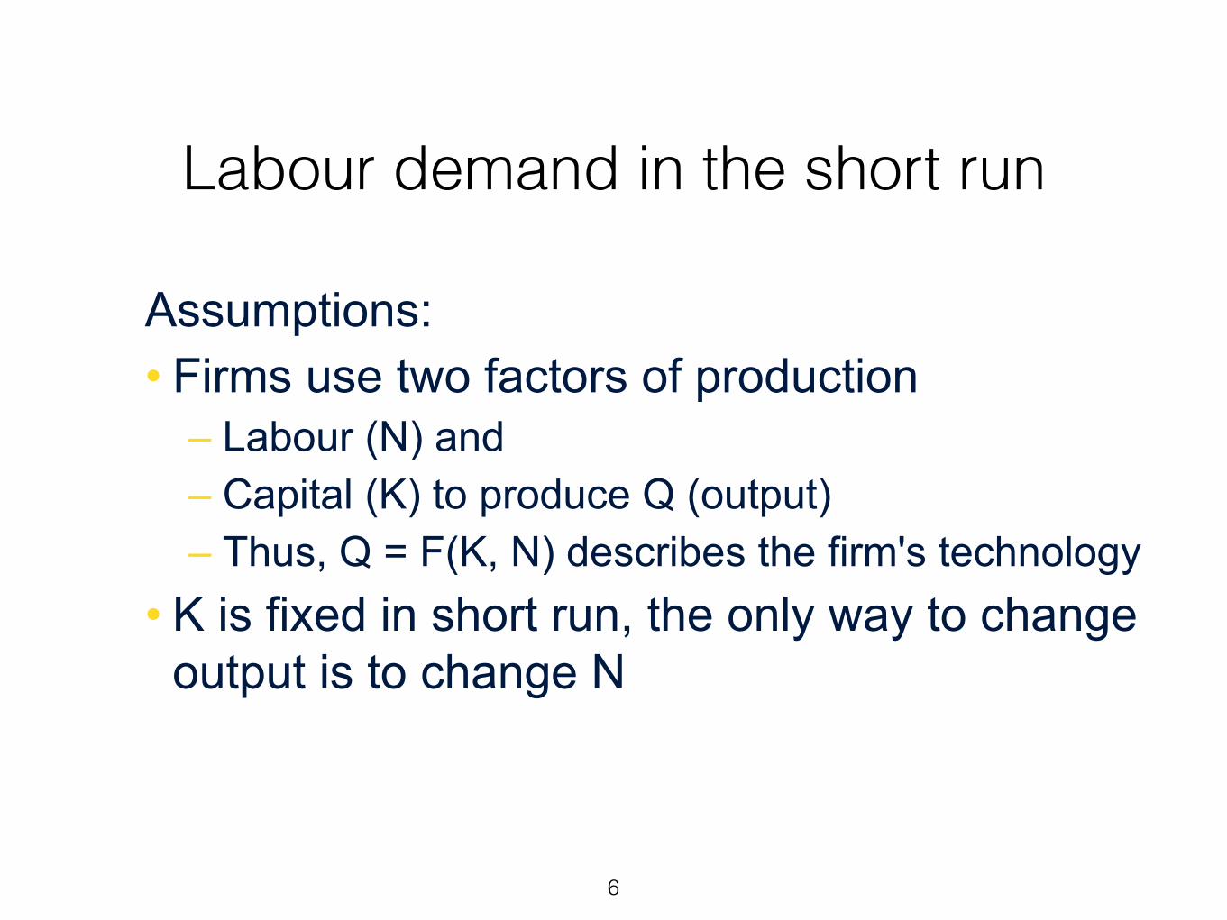
Assumptions: • Firms use two factors of production

– Labour (N) and – Capital (K) to produce Q (output) – Thus, Q = F(K, N) describes the firm's technology

• K is fixed in short run, the only way to change output is to change N


7

Firm is a profit maximizer. This implies two decision rules: 1. Shut Down: If total revenue is less than variable costs 2. How much to produce: If the firm does not shut down, it should produce where MC=MR.


8

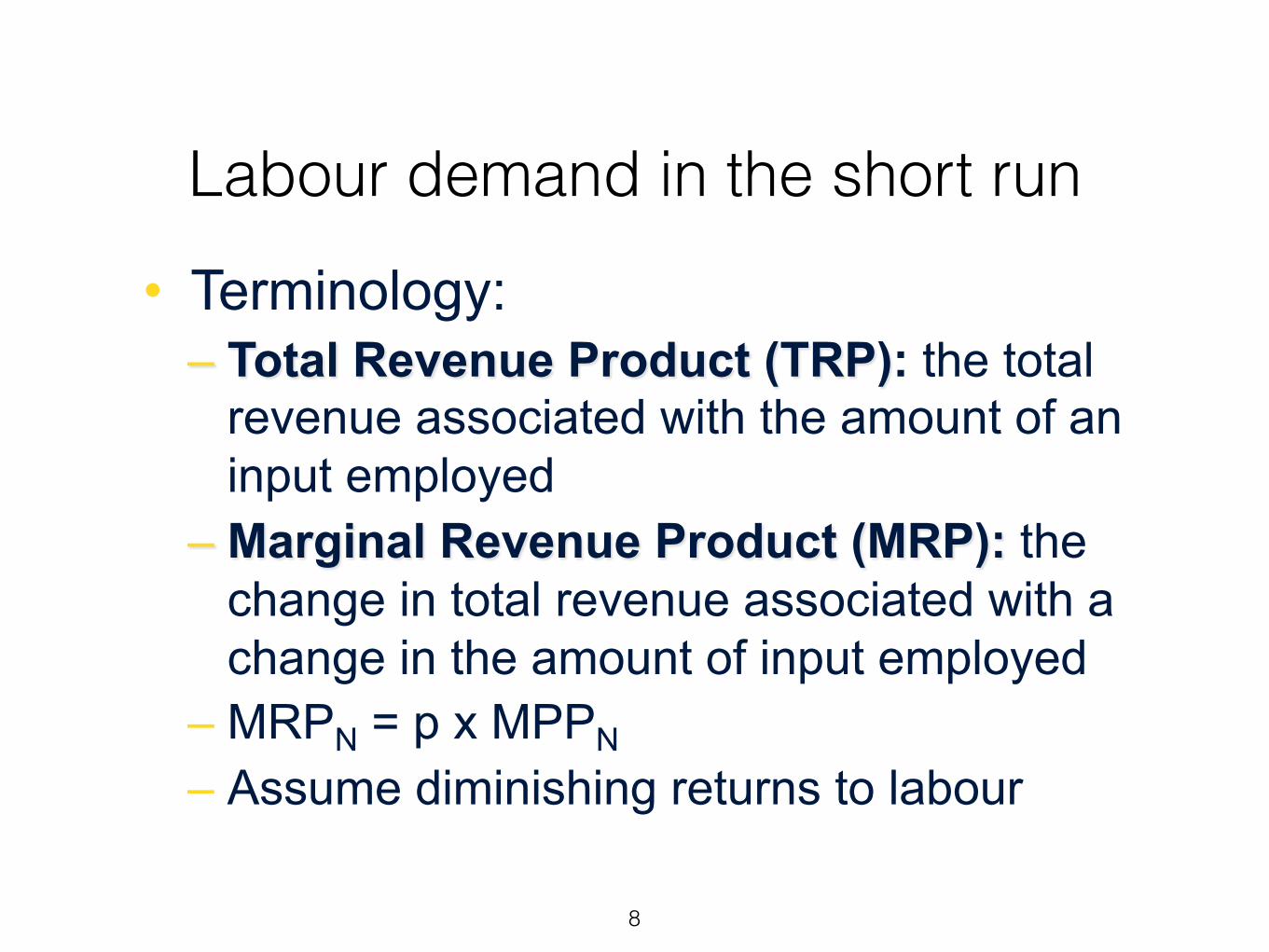
•  Terminology: – Total Revenue Product (TRP): the total

revenue associated with the amount of an input employed

– Marginal Revenue Product (MRP): the change in total revenue associated with a change in the amount of input employed

– MRPN = p x MPPN – Assume diminishing returns to labour


9

MRP N

N

Marginal Revenue Product of Labour

Average revenue product of labour

• Equals the total output (Q) divided by the total number of workers employed (N)

•  If the amount produced by adding an extra worker (MRP N) is greater than the average product (ARP N), then ARP N will rise

•  If MRP N < ARP N then ARP N falls

•  If MRP N = ARP N then no change

10

11

MRP N

N

MRP N ARP N

Finding the short run demand for labour

• A competitive firm will employ more labour until the value of the marginal product is just equal to the wage

• See handout 4

• A firm will shut down if the total revenue product of labour (ARPxN) is less than the total wage cost (w x N ) so that points on MRP N above the maximum ARP N will not be part of the demand schedule

12

14

•  Downward sloping because of diminishing marginal returns to labour

•  ↓ in wage rate will cause ↑ in demand for labour

•  ↑ in wage rate will cause ↓ in demand for labour


15

Labour Demand in the Long-Run All inputs are variable—no fixed costs

See handout 4

16

Labour Demand in the Long-Run

Isoquants:

•  “Equal quantity”

•  Combinations of labour and capital used to produce a given amount of a product (output)

•  Slope exhibits a diminishing marginal rate of technical substitution (MRTS)

17

Isoquants K

N 0

Q0

Q1

18

Labour Demand in the Long-Run

Isocost Line:

•  All combinations of capital and labour that can be bought for a given total cost

TC = rK + wN •  Where,

K = capital and N = labour r = price of capital w = wage

19

Isocost

N

K

c1/r0

C0 /r0

0 C0 /w0 c1/w0

Higher Cost

Lower Cost

20

Cost-Minimizing

N

K

0

K0

N1 N0

K1

Q0

E0

21

The long run labour demand is determined by the long run profit maximizing (cost minimizing) labour requirements such as point N0 in the previous diagram.

A Firm’s Labour Demand

22

The Impact of Wage Increases on Labour Demand

N

K C1/ r0

C0/ r0

0

Slope = -w0/r0

Slope = -w1/r0

Q1 Q0 K0

N0 C0/w0 C1/ w1 N1

●

E0

When wage rate changes from W0 to W1, E0 is no longer the profit maximizing equilibrium

The firm also re-evaluates output choices

23

Profit Maximizing Output and Derived Labour Demand

N

K

0 N0 NM

KM

Q0

E0

NM N1

E1

Q1

Slope = -w1/r0

Slope = -w0/r0

24

Derived Labour Demand Schedule

K

N 0

D

w1

w0

N1 N0

E0

E1

Points E0 and E1 correspond to profit maximizing long run equilibriums

25

The Effect of a Cost (Wage) Increase on Output Under Perfect Competition

•  ↑ wage rotates isocost line inwards •  The firm will maximize profit by reducing the

labour and substituting capital for labour •  ↑ wage also shifts up the firm's marginal and

average cost curves •  In a perfect competitive industry each firm

reduces output and raises the price of the product

26

The Effect of a Cost Increase on Output Under Perfect Competition

Price

Output

P1

P0

MC1 MC1

Q1 Q0

Firm

27

The Effect of a Cost Increase on Output Under Perfect Competition

Price

Output

P1

P0

S1 S0

q1 q0

D

Industry

28

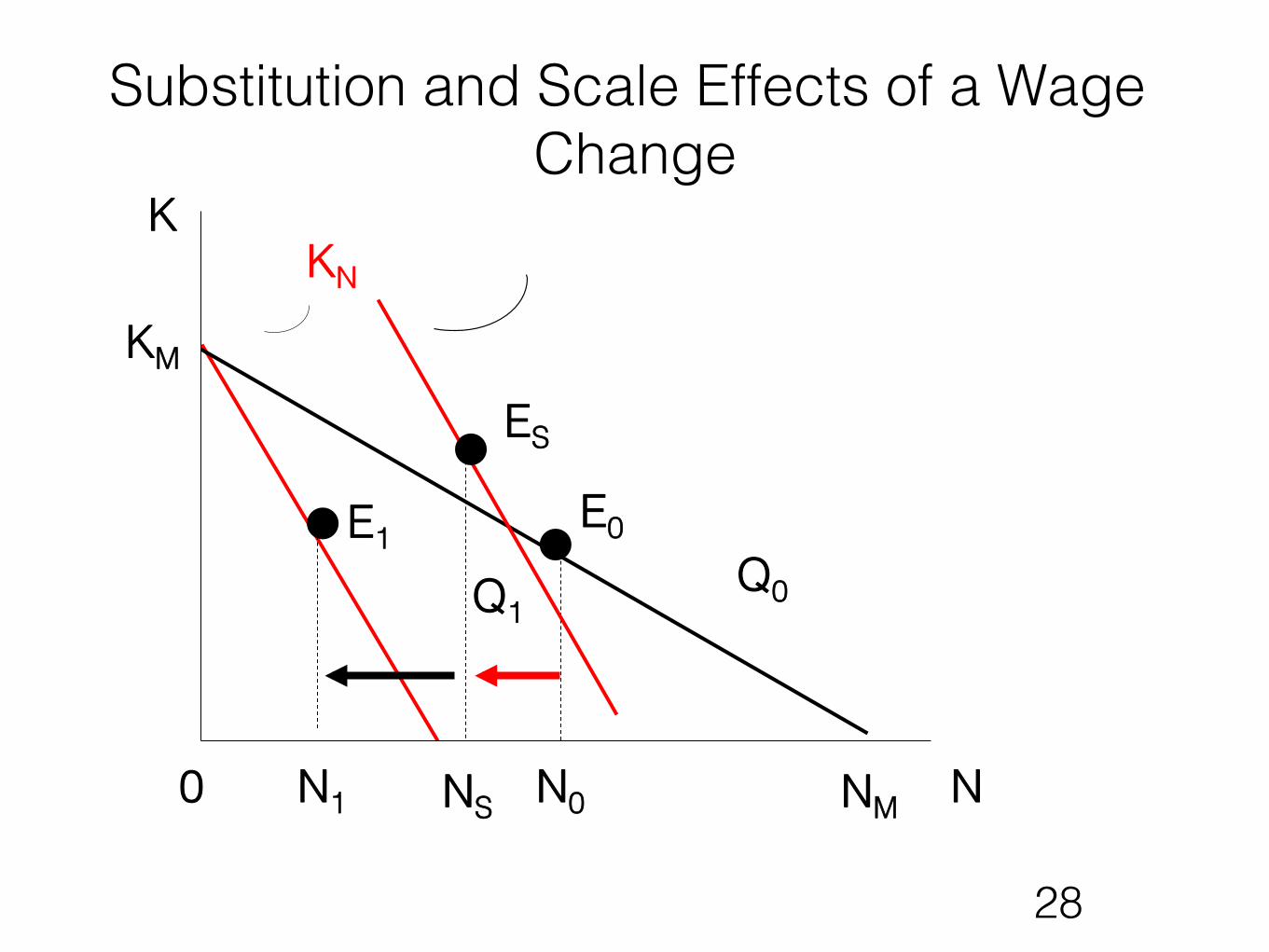
Substitution and Scale Effects of a Wage Change

N

K

0 NS N0 NM

KM

KN

Q0

E0

N1

E1

Q1

ES

29

Substitution and Scale Effects

•  Firm would substitute cheaper inputs for the more expensive labour:

•  SUBSITUTION EFFECT

•  Firm would reduce its scale of operations because of the cost increase associated with the increase in wage:

•  SCALE EFFECT

30

Short and Long Run

•  Short-Run •  amount of capital is fixed •  no substitution effect

•  Long-Run •  firm has flexibility by varying its capital stock •  response to a wage change will be larger in the long run

32

The Effect of a Cost Increase on Output Under Monopoly

Properties:

•  Single supplier •  No close substitute for the product •  Price setter •  Profit maximization conditions: MR = MC •  P > MC •  Firm and industry demands are the same •  When the monopolist hires more labour to

produce more output, both the marginal physical product of labour and the marginal revenue falls

•  MRPN = MR x MPPN = w

33

The Effect of a Cost Increase on Output Under Monopoly

Price

Output

P1

P0

MC1

MC0

q1 q0

D MR

34

Elasticity of Demand for Labour

• Demand for labour decreases as wages increase (negative function)

• Wage increases have an adverse effect on employment

• The magnitude of the effect can be seen by the elasticity of the derived demand for labour

35

Elasticity of Demand

• Measures the responsiveness of the quantity of labour demanded to the wage rate

• Equals the % change in the quantity of labour demanded divided by the % change in the wage rate

36

Elasticity of Demand for Labour

• Basic determinants of the elasticity of demand for labour:

• availability of substitute inputs

•  supply of substitute inputs

• demand for output

•  ratio of labour cost to total cost

37

Elasticity of Demand •  If inputs can not be easily substituted,

elasticity of labour demand decreases

•  If demand for output is not affected by a price increase (due to cost of wage increase) demand for labour will be inelastic

• Demand for labour will be inelastic if labour cost is small portion of total cost

38

Labour Demand and Globalization

• Outsourcing

• Trade

Outsourcing •  TC = WcNC + WFNF •  NC & NF substitutes •  Wc = 10 •  WF0 = 12.50 •  WF1 = 8 •  Substitution vs. scale

effects

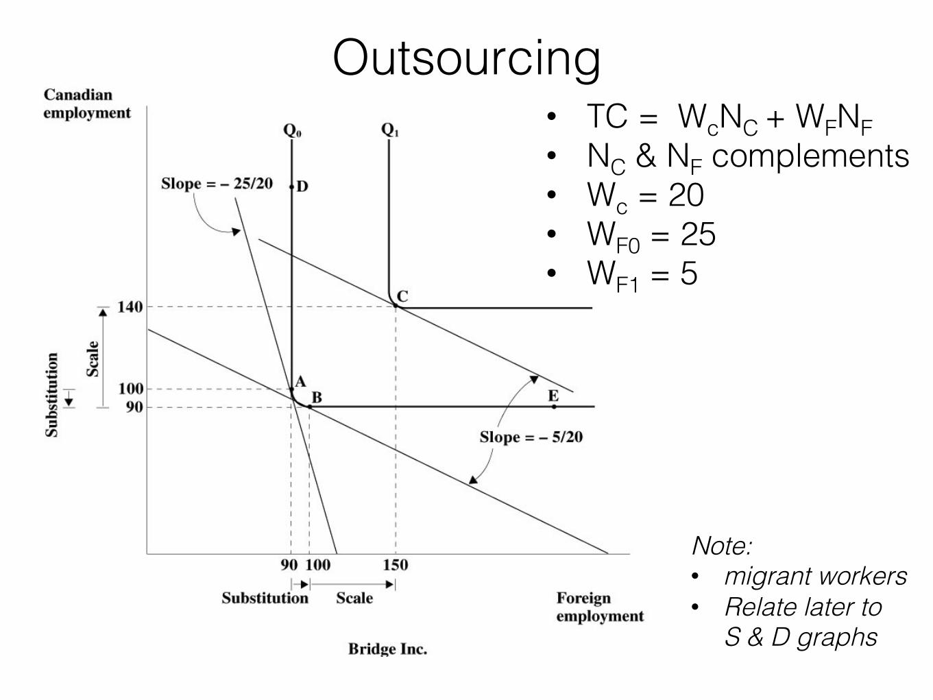
Outsourcing •  TC = WcNC + WFNF •  NC & NF complements •  Wc = 20 •  WF0 = 25 •  WF1 = 5

Note: •  migrant workers •  Relate later to

S & D graphs

Outsourcing •  Cost minimization implies

MRTS = MPPNC / MPPNF = WC / WF

•  Wage costs include trade barriers, WF reduced by ICTs

•  Both labour costs and productivity matter for the firms decisions

•  Consider isoquant for relatively productive Canadians (flat)

Source: ILC Tables, Productivity and Unit Labor Costs in Manufacturing, Data tables, 1950-2009, XLS file at http://www.bls.gov/fls/home.htm#productivity

Output per hour in manufacturing, average annual growth (%), 1979-2009


Hourly compensation in National currency (manufacturing), average annual growth (%), 1979-2009

Unit Labor Costs in National Currency (Mfg), average annual growth (%), 1979 - 2009


46

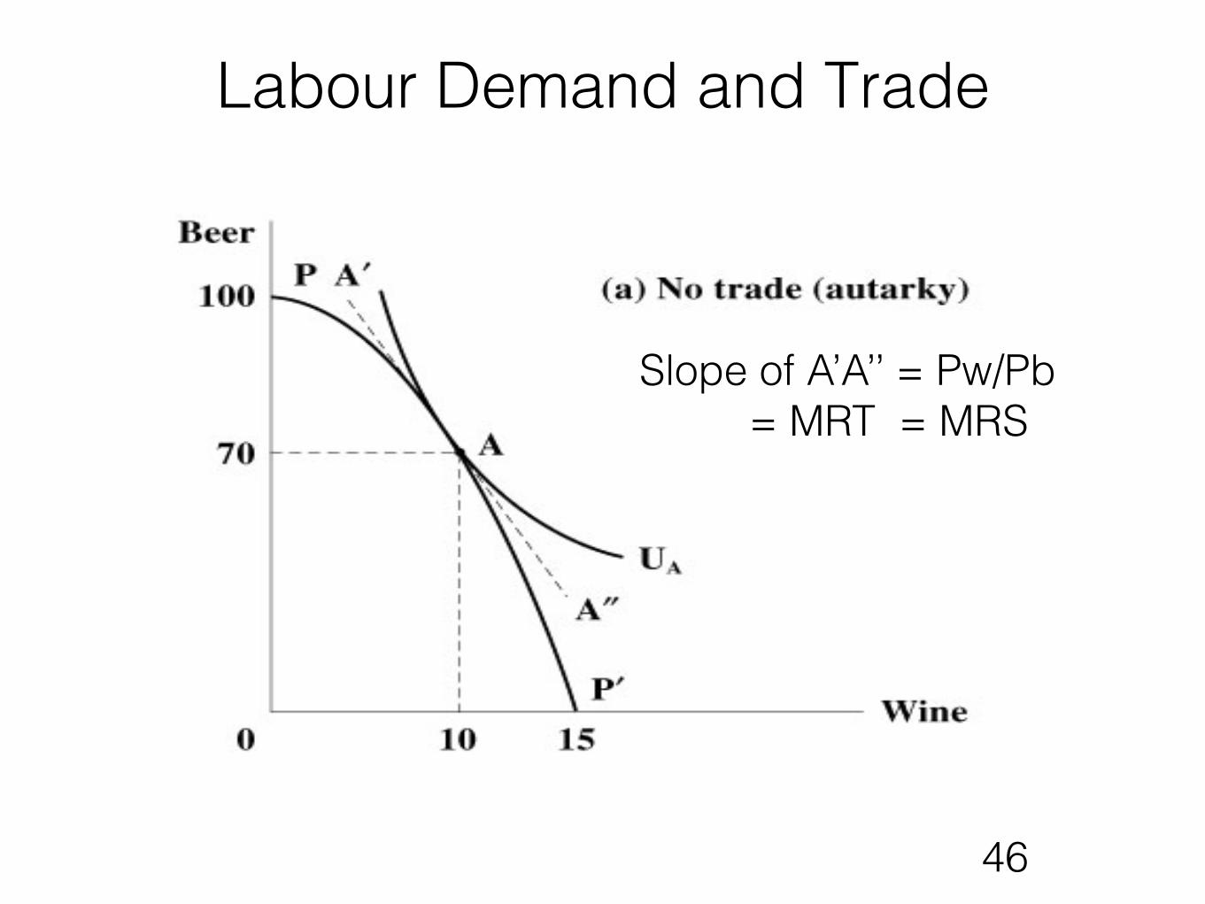
Labour Demand and Trade

Slope of A’A’’ = Pw/Pb = MRT = MRS

47


•  World prices matter, wine relatively cheaper

•  Sell beer to get wine •  Welfare improving

48



•  Increase in the overall welfare of the country

•  Distributional effects of globalization and trade:

•  What happens to the shrinking industry employees?

•  The case for wage insurance

49

Reading and references •  Required "

– BGLR Ch. 5"•  Suggested"

– The case for wage insurance by Robert J. Lalonde, http://www.cfr.org/economics/case-wage-insurance/p13661

50

ec306 labour economics - tammy schirle · • monopoly producers and labour demand ... maximizing...

Documents