1

EC3320 2016-2017 Michael Spagat

Lecture 6 For the Civilian Targeting Index (CTI) we merge together three datasets of the Uppsala Conflict Data Program:

1. UCDP Battle-Related Deaths Dataset – These are deaths in “battles” i.e., events where two armed groups fight each other. A quirk is that one of the armed groups has to be a state (i.e, a country) for deaths to qualify as battle deaths. Deaths from, for example, two tribes fighting get pushed into category 3 (below).

2. UCDP One-Sided Violence Dataset – These are deaths in events where one armed group does all the killing. These are intentional killings of civilians.

3. UCDP Non-State Conflict Dataset – These are basically the same as category 1 except that none of the groups involved in these incidents can be a state

2

The above descriptions are short and sweet. The reality of the coding is that it is complicated and there are many subtleties which I have to gloss over in this lecture. To go into more depth you can consult:

1. The “Materials and Methods” section of the CTI paper.

2. The “Crunching Corpse Counts…” blog post.

3

We organize everything by group. For each group in each year, 2002-2007 we have battle deaths, one-sided deaths (civilian targeting) and non-state deaths. There are also a few pieces of basic information such as where the group operates and whether or not it is a state group. There are 226 groups, of which 43 are state groups and 183 are non-state groups. The CTI for each group is defined as:

100xdeathsnonstatedeathsbattledeathssidedOne

deathssidedOne++−

−

In other words, the CTI for a group is simply the percentage of total deaths associated with the group that are one-sided deaths (i.e., intentional civilian targeting). So, for example, if a group has a CTI of 100 then this group has only one-sided deaths on its account. If the CTI is 0 then the group has only battle and/or non-state deaths. When the CTI is between 0 and 100 then there are both one-sided deaths and battle/non-state deaths.

4

5

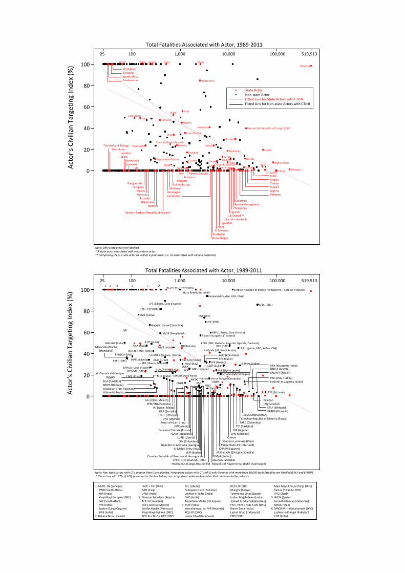
The picture on slide 4 plots the total number of direct fatalities associated with an actor (from battle-deaths and civilian targeting) against the proportion of total fatalities that was from the actor's civilian targeting, termed the Civilian Targeting Index (CTI). Lines show fitted linear regressions for state actors (in red) and non-state actors (in black) that carried out at least some civilian targeting (actor's CTI>0). Actors in the upper-right corner of the picture are isolated as the worst performers. You can inspect the graph in minute detail if you view it online at PLoSOne (click on “View all figures” and then down load the original image as a TIFF file). Or you can just magnify the pdf of these lecture notes.

6

Here are some key take-home points:

First, the majority (61%) of all formally organized actors in armed conflict during 2002-2007 refrained from killing civilians in deliberate, direct targeting. This comes straight from looking at the data.

Second, actors were more likely to have carried out some degree of civilian targeting (CTI >0), as opposed to none (CTI = 0), if they participated in armed conflict for three or more years rather than for one year. This comes from logistic regression (Table 4 in the paper), which, as we have seen, is basically like usual regression but adapted to the case for which the left-hand-side variable can take on just two possible values (in this case CTI > 0 or CTI = 0). Note that this result says nothing about the extent to which groups target civilians once they have done so at least once (i.e., “crossed the line” into civilian targeting).

Third, among actors that targeted civilians (there were 88 of them), those that engaged in greater scales of armed conflict concentrated less of their lethal behavior into civilian targeting and more into involvement with battle fatalities. Also, those engaged for more than three years tended to have lower CTI’s.

Fourth, an actor's likelihood and degree of targeting civilians was unaffected by whether it was a state or a non-state group.

7

These last two points just follow from the regression lines shown in figure 1 and spelled out in Table 6 of the paper. They suggest that there is a tradeoff between targeting civilians and engaging in battle. An armed group may attempt to control territory by terrorizing, and hence controlling the civilian population. Alternatively, an armed group may try to control the territory by dominating competing armed groups attempting to operate in the area.

As part of her PhD dissertation here at RHUL Uih Ran Lee updated the main picture and analysis for the PLoSOne paper (next slide).

Afghanistan

Burundi

Cameroon

Central African Republic

ChadCongo-Brazzaville

Cote d’Ivoire

Croatia

Democratic Republic of Congo (DRC)

Egypt

Guatemala

Guinea

Haiti

Indonesia

IraqIsrael

Laos

Liberia

Mali

Myanmar

Nepal

Niger

Nigeria

Papua New Guinea

Romania

Russia

Rwanda

Senegal

Serbia

Somalia

SudanThailand

US

Venezuela

Sierra LeoneEthiopia

Sri LankaEritrea

Brazil ChinaKenyaLibya Togo

0

20

40

60

80

100A

cto

r's

Civ

ilia

n T

arg

eti

ng

In

de

x (%

)

Total Fatalities Associated with Actor 1989-2011

ADF (Uganda)

AFDL (DRC)

Al-Qaida (US, Saudi Arabia)

AMB (Israel)

ATTF (India)DHD-BW (India)

FAPC (DRC)

FARF (Chad)

FDLR (DRC, Rwanda, Burundi, Uganda, Tanzania)FIAA (Mali)

FNI (DRC)

FNI + FRPI (DRC)

FPR (Rwanda)INPFL (Liberia)

ISI (Iraq, Jordan)

Janjaweed (Sudan, CAR, Chad)

JSS/SB (Bangladesh)

Khmer Rouge (Cambodia)

LPC (Liberia, Cote d'Ivoire)

LRA (Uganda, DRC, Sudan, CAR)

MCC (India)

Medellin Cartel (Colombia)

MPCI (Cote d’Ivoire)

MPIGO (Cote d'Ivoire)

NDFB (India)NLFT (India)

NPFL (Liberia, Cote d’Ivoire)

NSCN-IM (India)

PARECO (DRC)

Patani Insurgents (Thailand)

RCD (DRC)

RCD-ML (DRC)

RCD-N + MLC (DRC)

Renamo (Mozambique)

RUF (Sierra Leone)

SLDF (Kenya)

SLM/A-MM (Sudan)

SSDF (Sudan)ULIMO (Liberia, Guinea)

ULIMO-K (Guinea, Liberia)

UPC (DRC)

LTTE (Sri Lanka)

Serbian Republic of Bosnia-Herzegovina + Serbian IrregularsHutu Rebels (Burundi)

RCD-K-ML + FRPI (DRC)

0

20

40

60

80

100

Act

or'

s C

ivil

ian

Ta

rge

tin

g I

nd

ex

(%)

Total Fatalities Associated with Actor 1989-2011

Zimbabwe

Tanzania

South Africa

Madagascar

1. MFDC-FN (Senegal)

AWB (South Africa)

KRA (India)

Mayi Mayi Complet (DRC)

PAC (South Africa)

HPC (India)

Buxton Gang (Guyana)

SIMI (India)

2. Bakassi Boys (Nigeria)

India

Angola

Turkey

Kuwait

Algeria

Pakistan

Trinidad and Tobago

Mauritania

Bangladesh

Paraguay

Mexico

Morocco

Ecuador

Uzbekistan

Djibouti

Tajikistan

Peru

El Salvador

Azerbaijan

Mozambique

Serbia + Serbian Republic of Krajina*

Georgia

UIFSA (Afghanistan)

Chechen Republic of Ichkeria (Russia)

Colombia

Bosnia-Herzegovina

Philippines

Uganda

US Overall**

US + UK + Australia

25 100 1,000 10,000 100,000 519,513

Lesotho

Spain

Macedonia

Comoros

UK

Iran Yemen

Lebanon

Panama

Guinea-Bissau

Moldova

Nicaragua

Note: Only state actors are labelled.

* A state actor associated with a non-state actor

** Comprising US as a sole actor as well as a joint actor (i.e. US associated with UK and Australia)

Al-Gama'a al-Islamiyya

(Egypt)

Mara Salvatrucha

(Honduras)

JVP

Sikh Insurgents (India) Mayi Mayi

Los Zetas (Mexico)

SPM/SNA (Somalia)

PIJ (Israel, Malta)

RRA (Somalia)

ONLF (Ethiopia)

UPA (Uganda)

Ansar al-Islam (Iraq)

PWG (India)

Caucasus Emirate (Russia)

GAM (Indonesia)

LURD (Liberia)

ELN (Colombia)

Republic of Abkhazia (Georgia)

Al-Mahdi Army (Iraq)

JEM (Sudan)

Croatian Republic of Bosnia and Hercegovina

CNDD-FDD (Burundi, DRC)

Ntsiloulous (Congo-Brazzaville)

BLA (Pakistan)

NDFB-RD (India)

Jondullah (Iran, Pakistan)

Ulimo-J (Liberia)

CNDP

MFDC Hamas

ASG MILF

PKK (Iraq, Turkey)

Kashmir Insurgents (India)

ULFA

JVP

AUC (Colombia)

CPI-Maoist

FARC (Colombia)

TTP (Pakistan)

GIA (Algeria)

CPN-M (Nepal)

Cobras

Sendero Luminoso (Peru)

Palipenhutu-FNL (Burundi)

CPP (Philippines)

Al Shahaab (Ethiopia, Somalia)

SLM/A (Sudan)

USC/SSA (Somalia)

Republic of Nagorno-Karabakh (Azerbaijan)

KNU

Taleban

(Afghanistan)

EPLF (Ethiopia)

EPRDF (Ethiopia)

UNITA (Angola)

SPLM/A (Sudan)

AQIM

Cambodia

25 100 1,000 10,000 100,000 519,513

,

,

1 2 3 4 5 6*

Note: Non-state actors with CTIs greater than 0 are labelled. Among the actors with CTIs of 0, only the ones with more than 10,000 total fatalities are labelled (EPLF and EPRDF).

* The actors with CTIs of 100, presented in the box below, are categorised under each number that are bounded by red dots.

FAPC + FNI (DRC)

AAH (Iraq)

UPDS (India)

3. Gazotan Murdash (Russia)

ACCU (Colombia)

Paz y Justicia (Mexico)

Salafia Jihadia (Morocco)

Mayi Mayi-Ngilima (DRC)

RCD-N + MLC + UPC (DRC)

AFL (Liberia)

Fedayeen Islam (Pakistan)

Lashkar-e-Taiba (India)

DHD (India)

Ampatuan Militia (Philippines)

4. BLTF (India)

Interahamwe, ex-FAR (Rwanda)

RCD-CP (DRC)

Laskar Jihad (Indonesia)

RCD-LN (DRC)

Mungiki (Kenya)

Tawhid wal Jihad (Egypt)

Indian Mujahideen (India)

Jamaat Jund al-Sahaba (Iraq)

FNI + FRPI + RCD-K-ML (DRC)

Ranvir Sena (India)

Laskar Jihad (Indonesia)

FRPI (DRC)

Mayi Mayi-Chinja Chinja (DRC)

Rastas (Rwanda, DRC)

RTC (Chad)

5. GICM (Spain)

Jemaah Islamiya (Indonesia)

MPGK (Mali)

6. MAGRIVI + Interahamwe (DRC)

Lashkar-e-Jhangvi (Pakistan)

VHP (India)

• State Actor

• Non-state Actor

Fitted Line for State Actors with CTI>0

Fitted Line for Non-state Actors with CTI>0

9

More Insight into Logistic Regression

Recall that the standard linear regression framework is designed for cases where the left-hand-side variable can take any value. Logistic regression is for cases where the left-hand-side variable can take only two values, normally rendered as 0 and 1. Slide 6 referred to a logistic regression in which “0” corresponds to a CTI of 0 and “1” corresponds to a CTI > 0 which I referred to as “crossing the line” into doing at least some civilian targeting. Here I want to explore quickly the difference between a linear probability model, i.e., a linear regression approach, and a logistic regression approach for this “crossing-the-line” question.

10

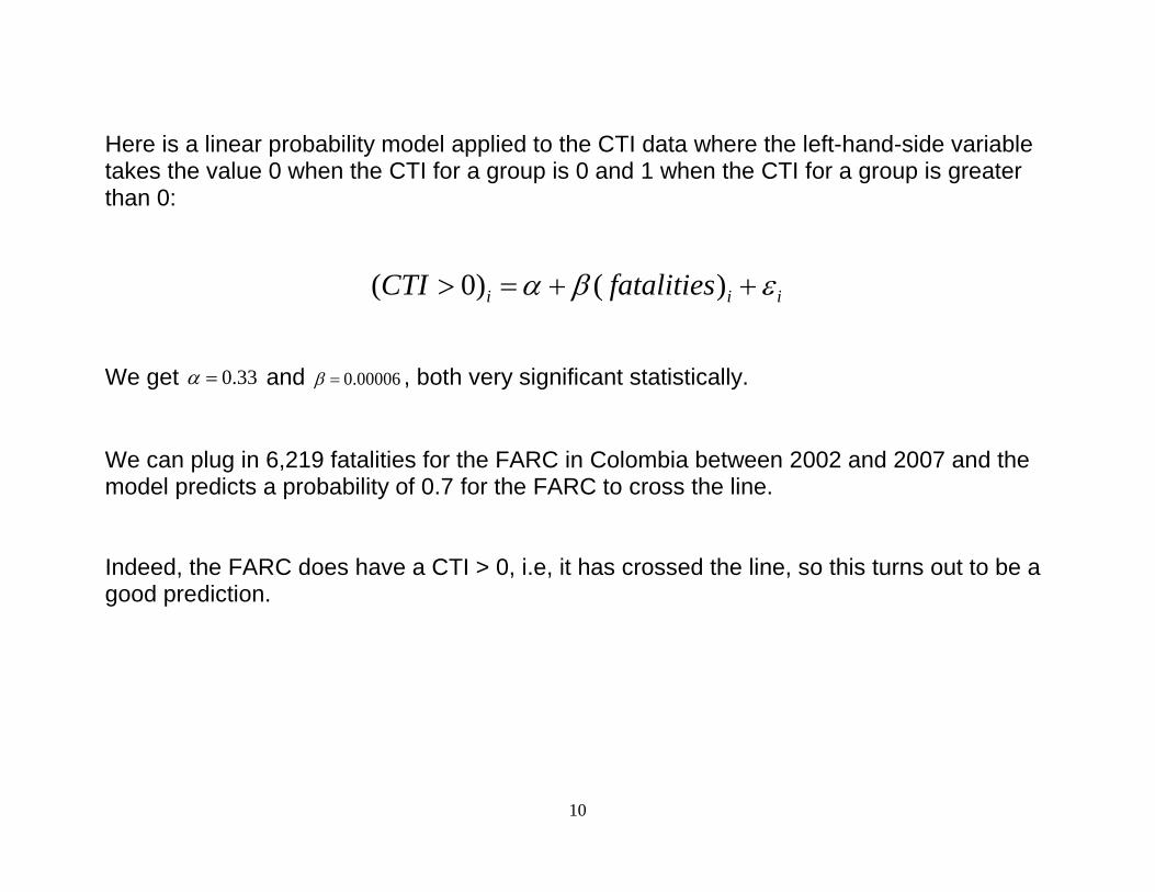
Here is a linear probability model applied to the CTI data where the left-hand-side variable takes the value 0 when the CTI for a group is 0 and 1 when the CTI for a group is greater than 0:

iii fatalitiesCTI eβa ++=> )()0( We get 33.0=a and 00006.0=β , both very significant statistically. We can plug in 6,219 fatalities for the FARC in Colombia between 2002 and 2007 and the model predicts a probability of 0.7 for the FARC to cross the line. Indeed, the FARC does have a CTI > 0, i.e, it has crossed the line, so this turns out to be a good prediction.

11

There are, however, some problems with this linear probability model. Consider, for example, our old friend Iraq. The government of Iraq has 19,956 fatalities associated with it in the data. Plugging this into the equation we end up predicting the probability that Iraq has targeted civilians is…..1.53…. Of course, this makes no sense because probabilities have to be between 0 and 1. We could, however, paper over this problem by resetting our prediction to 1 whenever the prediction exceeds 1. The adjustment would work in the present case since Iraq has, indeed, targeted civilians. The CTI data contain three more cases for which “probabilities” are above 1 and in each oneone the CTI is greater than 0. So this adjustment method works well in all these cases. In other linear probability models predicted “probabilities” can fall below 0 but this does not happen with the CTI data.

12

Of course the logistic model guarantees that predictions are between 0 and 1 so it does this work for us. Using the same CTI data as above we use logistic regression to estimate 82.0−=a and

00041.0=β . The prediction for the FARC, with 6,219, fatalities is:

85.01

1)621900041.082.0( =

+ +−− xe

This is noticeably higher than what we got before (0.7). Both predictions have to be considered good for a variable that turns out to be 1 although the higher number given by the logistic has to be considered a better prediction for this case. For Iraq the prediction comes out bang on 1.0. This is certainly an improvement although it is not clear that it is a big one, given that we were adjusting all the predictions above 1.0 so that they equal 1.0 anyway.

13

I did manage to find a slight advantage for logistic regression with these data. To understand the advantage we will apply a common and simple forecasting rule, using both models. 1. If a model gives a predicted probability of crossing the line that is bigger than 0.5 and the group actually does cross the line we will call that a successful prediction. If the probability is bigger than 0.5 and the group does not cross the line we will call that an unsuccessful prediction. 2. Predictions below 0.5 are successes if and only if the group does not cross the line. Using this prediction method the linear probability model (old fashioned regression) makes correct predictions for 152 out of the 229 groups. The logistic model makes correct predictions for 153 out of 229…..better but not exactly a spectacular triumph.

14

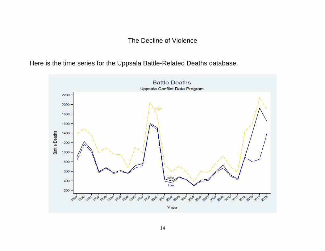
The Decline of Violence

Here is the time series for the Uppsala Battle-Related Deaths database.

15

I used to observe at this point in the lecture that there is an irregular downward trend. However, now that 2014-15 has been added in this is no longer true. Now I would say that there has been no real trend since 1989.

16

What about one-sided deaths?

This picture gives us an unexpected lesson in graphical displays. The Rwandan genocide is gigantic compared to all the other numbers. This stretches the y axis so much that the number of one-sided deaths in every year other than 1994 looks pretty much indistinguishable from 0. Our eyes are not good enough to spot a trend.

17

We address this visual issue by logging the y axis:

18

The point of logging the y axis is to make good use of all the space in the picture so that things are happening everywhere in the picture instead of just at the very bottom and at the very top of the picture. As with battle death you could see general movement down until 2013-14. The Rwandan genocide complicates this picture. Perhaps it is just a one off or perhaps there will, periodically, be major events like it in the future.

19

The PRIO Battle Deaths Dataset

There is an alternative to the Uppsala Battle Deaths dataset. It is called the PRIO Battle Deaths Dataset. Why do we need an alternative battle deaths dataset?

1. The PRIO dataset goes back to 1946. (Actually it goes back to World War 1 but the quality is lower before 1946 than it is after 1946 so we do not use it hear.) Uppsala only goes back to 1989 because they record incident level data and they cannot maintain what they view as a high enough standard going back any further than they do.

2. PRIO has much less stringent criteria than Uppsala has so it is interesting to have a

different set of numbers based on more flexible data gathering practices. (PRIO will accept things such as estimates [guestimates?] of historians or former military officers. Uppsala also excludes various types of incidents such as those with unknown perpetrators.)

20

The battle-deaths time series for the PRIO Battle Deaths Dataset is on the next slide. Researchers assemble these data by looking at all possible sources they can find on every conflict in the world. The sources are evaluated in each case and the researchers make their best estimates of battle deaths.

21

It is quite irregular but it still generally goes down over time. If we added World War II then the long-term decline would be more pronounced than what you see above.

22

So taking a longer view suggests that war is declining. The Obermeyer et al. paper (I will refer to it as “OMG” below) disputes the proposition that war is declining.

“War causes more deaths than previously estimated…” “…media estimates capture on average a third of the number of deaths estimated from population based surveys.”

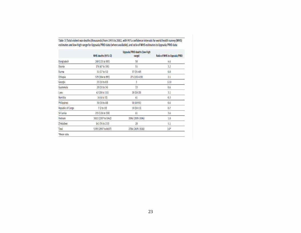
In particular, OMG claim that the PRIO battle deaths data underestimate deaths by a factor of three on average. The evidence for this claim in summarized in table 3 on the next slide with the key number being the 3.0 at the bottom-right of the table. Have a quick look at the table on the next slide and tell me if it triggers any memories.

23

24

The PRIO battle death figures are given in the column (incorrectly) called “Uppsala/PRIO deaths (low-high range). (The Uppsala/PRIO dataset is different from the PRIO battle deaths dataset.) The column called “WHS deaths” is based on surveys that were done in many countries called the “World Health Surveys”. These are similar to the types of surveys we discussed for measuring conflict deaths (lecture 3). (The only difference is that the WHS surveys try to measure deaths by asking people about their siblings, i.e., are they alive or dead and if they are dead were they killed violently? This means that calculations are done differently than are the calculations in the household surveys we discussed in lecture 3 and elsewhere but we will not discuss these calculations here. Instead, we will largely just assume that the measurements given in the table are accurate.)

25

Problems with the claims quoted on slide 22. 1. PRIO numbers are not actually media based. (Recall - “…media estimates capture on average a third of the number of deaths estimated from population based surveys.”) In some cases media surveillance underpins a source used by PRIO but, in general, these numbers have very little to do with media surveillance. So even if the PRIO figures are truly too low by a factor of three this in no way suggests that media surveillance tends to produce figures that are too low by a factor of 3.

26

2. The table above suggests that a ratio of 2 to 1 is more accurate than 3 to 1.

a. The 3.0 comes from taking the mean of the 13 ratios across the 13 countries. Some of these conflicts are much larger than others but they all get weighted equally in this averaging. In particular the small conflict in Georgia gets the same weight as the huge conflict in Viet Nam. If, instead, you weight each death (rather than each of the 13 ratios) equally then the ratio comes out 5393/2784 = 1.9, not 3.0 (table 3 above).

b. If you take the median of the 13 ratios, rather than the mean, then you get a ratio of 2.1 (table 3 above)

27

3. OMG use a “war deaths” concept which is wider than PRIO’s “battle deaths” concept. War deaths correspond roughly to battle deaths plus non-state deaths plus one-sided deaths. So, up to a point, it is not a deficiency of the PRIO data to be lower than the OMG data. 4. OMG throw away data from 23 further countries where the World Health Surveys measured essentially 0 deaths. In other words, they have a biased sample. So, in fact, most of the time the PRIO figures are actually higher than the OMG ones but OMG claim the opposite. I think these problems are terminal, i.e., the OMG claim is simply false.

28

The second key claim of OMG is that “there is no evidence to support a recent decline in war deaths.” This claim is based on a somewhat complicated transformation of the PRIO time series that was displayed in slide 21 (above). The basic idea is that the PRIO numbers are incomplete and so some upward adjustment is necessary to make them realistically represent the true situation.

29

This transformation cannot be to just multiply all PRIO numbers by a fixed constant (such as OMG’s factor of 3.0) because doing this would just shift all numbers up without changing any trends. To change the trends you need to do something more complicated than that. So what do OMG do? They run a regression using the data from columns 2 and 3 of table 3 above, getting:

WHS Deaths = 27,380 + 1.81 x PRIO Deaths

30

Because of the constant term (27,380) this transformation does have the potential to change time trends. Imagine for example that you have two years of data. In the first year there is one conflict with 10,000 battle deaths. In the second year there are two conflicts, each with 1,000 battle deaths. According to PRIO there would be a downward trend from 10,000 in the first year to 2,000 in the second year. According to OMG there would be an upward trend with 45, 480 in the first year (27,380 + 1.81 x 10,000) and 58, 380 in the second year (27,380 + 1.81 x 1,000 + 27, 380 + 1.81 x 1,000). So applying this regression transformation to the PRIO data completely reverses the trend.

31

OMG do this to a big piece of the PRIO data and get the following picture:

Source: Obermeyer et al. paper

32

They do not claim that this picture shows an upward trend but, rather, that there is no evidence of a downward trend. One thing is immediately very curious in this picture – the dates only cover 1955 – 94. Have a look at the picture on slide 21 and ask yourself about the implications of cutting the time series in this way.

33

Moreover, I do not agree with this transformation procedure. Recall from the last slide that the 27,380 constant is crucial for changing trends. But look at the following plot of the data that the regression is performed on.

34

Does the red regression line look like it hits the y axis at 27,300? It does actually hit there but you can’t see this with the naked eye due to the scale of the picture. In fact, this estimated coefficent is not statistically significant and isn’t even close to being statistically significant. The 95% confidence interval around it is about -19,000 to 73,616. Really, the whole idea of taking seriously a regression on just 13 points is silly and in this case it’s more like OMG have only 3 points: Vietnam, Ethiopia and a blob of points near the origin. The OMG transformation is not convincing. To summarize I would say that the whole OMG critique of the decline-of-war thesis is useless.