eccv deep dynamic neural networks for gesture … · previous works on video-based motion...
TRANSCRIPT

000
001
002
003
004
005
006
007
008
009
010
011
012
013
014
015
016
017
018
019
020
021
022
023
024
025
026
027
028
029
030
031
032
033
034
035
036
037
038
039
040
041
042
043
044
000
001
002
003
004
005
006
007
008
009
010
011
012
013
014
015
016
017
018
019
020
021
022
023
024
025
026
027
028
029
030
031
032
033
034
035
036
037
038
039
040
041
042
043
044
ECCV
#ECCV
#
Deep Dynamic Neural Networks for GestureSegmentation and Recognition
Di Wu, Ling Shao
The University of [email protected], [email protected]
Abstract. The purpose of this paper is to describe a novel methodcalled Deep Dynamic Neural Networks(DDNN) for the Track 3 of theChalearn Looking at People 2014 challenge [1]. A generalised semi-supervisedhierarchical dynamic framework is proposed for simultaneous gesturesegmentation and recognition taking both skeleton and depth images asinput modules. First, Deep Belief Networks(DBN) and 3D ConvolutionalNeural Networks (3DCNN) are adopted for skeletal and depth data ac-cordingly to extract high level spatio-temporal features. Then the learnedrepresentations are used for estimating emission probabilities of the Hid-den Markov Models to infer an action sequence. The framework can beeasily extended by including an ergodic state to segment and recognisevideo sequences by a frame-to-frame mechanism, rendering it possiblefor online segmentation and recognition for diverse input modules. Somenormalisation details pertaining to preprocessing raw features are alsodiscussed. This purely data-driven approach achieves 0.8162 score inthis gesture spotting challenge. The performance is on par with a varietyof the state-of-the-art hand-tuned-feature approaches and other learning-based methods, opening the doors for using deep learning techniques toexplore time series multimodal data.
Keywords: Deep Belief Networks, 3D Convolutional Neural Networks,Gesture Recognition, ChaLearn
1 Introduction
In recent years, human action recognition has drawn increasing attention ofresearchers, primarily due to its growing potential in areas such as video surveil-lance, robotics, human-computer interaction, user interface design, and multi-media video retrieval.
Previous works on video-based motion recognition focused on adapting hand-crafted features and low-level hand-designed features [2,3,4] have been heav-ily employed with much success. These methods usually have two stages: anoptional feature detection stage followed by a feature description stage. Well-known feature detection methods (“interest point detectors”) are Harris3D [5],Cuboids [6] and Hessian3D [7]. For descriptors, popular methods are Cuboid-s [8], HOG/HOF [5], HOG3D [9] and Extended SURF [7]. In a recent work of

045
046
047
048
049
050
051
052
053
054
055
056
057
058
059
060
061
062
063
064
065
066
067
068
069
070
071
072
073
074
075
076
077
078
079
080
081
082
083
084
085
086
087
088
089
045
046
047
048
049
050
051
052
053
054
055
056
057
058
059
060
061
062
063
064
065
066
067
068
069
070
071
072
073
074
075
076
077
078
079
080
081
082
083
084
085
086
087
088
089
ECCV
#ECCV
#
2 Di Wu, Ling Shao
Wang et al. [10], dense trajectories with improved motion-based descriptors epit-omized the pinnacle of handcrafted features and achieved state-of-the-art resultson a variety of “in the wild” datasets. Given the current trends, challenges andinterests in action recognition, this list would probably continue to spread outextensively. The very high-dimensional dense-trajectory features usually requireadvanced dimensionality reduction techniques [11,12] to make them applicable.
In the evaluation paper of Wang et al. [13], one interesting finding is thatthere is no universally best hand-engineered feature for all datasets, suggestingthat learning features directly from the dataset itself may be more advantageous.Albeit the dominant methodology for visual recognition from images and videosrelies on hand-crafted features, there has been a growing interest in methodsthat learn low-level and mid-level features, either in supervised, unsupervised,or semi-supervised settings [14,15,16].
With the recent resurgence of neural networks invoked by Hinton and oth-ers [17], deep neural architectures have been proposed as an effective solutionfor extracting high level features from data. Deep artificial neural networks (in-cluding the family of recurrent neural networks) have won numerous contestsin pattern recognition and representation learning. Schmidhuber [18] compileda historical survey compactly summarising relevant works with more than 850entries of credited works. Such models have been successfully applied to a pletho-ra of different domains: the GPU-based cuda-convnet [19] classifies 1.2 millionhigh-resolution images into 1000 different classes; multi-column Deep NeuralNetworks [20] achieve near-human performance on the handwritten digits andtraffic signs recognition benchmarks; 3D Convolutional Neural Networks [21,22]recognize human actions in surveillance videos; Deep Belief Networks combiningwith Hidden Markov Models [23,24] for acoustic and skeletal joints modeling out-perform the decade-dominating paradigm of Gaussian Mixture Models+HiddenMarkov Models. In these fields, deep architectures have shown great capacity todiscover and extract higher level relevant features.
However, direct and unconstrained learning of complex problems is difficult,since (i) the amount of required training data increases steeply with the com-plexity of the prediction model and (ii) training highly complex models withvery general learning algorithms is extremely difficult. It is therefore commonpractice to restrain the complexity of the model and this is generally done byoperating on small patches to reduce the input dimension and diversity [16], orby training the model in an unsupervised manner [15], or by forcing the mod-el parameters to be identical for different input locations (as in convolutionalneural networks [19,20,21]).
With the immense popularity of Kinect [25,26], there has been renewed in-terest in developing methods for human gesture and action recognition from 3Dskeletal data and depth images. A number of new datasets [27,28,29,30] haveprovided researchers with the opportunity to design novel representations andalgorithms and test them on a much larger number of sequences. It may seemthat the task of action recognition given 3D joint positions is trivial, but thisis not the case, largely due to the high dimensionality of the pose space. Fur-
090
091
092
093
094
095
096
097
098
099
100
101
102
103
104
105
106
107
108
109
110
111
112
113
114
115
116
117
118
119
120
121
122
123
124
125
126
127
128
129
130
131
132
133
134
090
091
092
093
094
095
096
097
098
099
100
101
102
103
104
105
106
107
108
109
110
111
112
113
114
115
116
117
118
119
120
121
122
123
124
125
126
127
128
129
130
131
132
133
134
ECCV
#ECCV
#
Deep Dynamic Neural Networks for Gesture Segmentation and Recognition 3
thermore, to achieve continuous action recognition, the sequence need to besegmented into contiguous action segments; such segmentation is as importantas recognition itself and is often neglected in action recognition research.
In this paper, a data driven framework is proposed, focusing on analysis ofacyclic video sequence labeling problems, i.e., video sequences are non-repetitiveas opposed to longer repetitive activities, e.g., jogging, walking and running.
2 Experiments and Analysis
2.1 Chalearn LAP Dataset & Evaluation Metrics
This dataset1 is on “multiple instance, user independent learning and continuousgesture spotting” [27] of gestures. And in the 3 track, there are more than 14,000gestures are drawn from a vocabulary of 20 Italian cultural/anthropological signgesture categories with 700 sample sequences for training and validation and 240sample sequences for testing.
The evaluation criteria for this track is the Jaccard index (overlap) on aframe-to-frame basis.
J(A,B) =A⋂B
A⋃B
(1)
2.2 Model Architecture: Deep Dynamic Neural Networks
Inspired by the framework successfully applied to the speech recognition [23],the proposed model borrows the idea of a data driven learning system, relyingon a pure learning approach in which all the knowledge in the model comes fromthe data without sophisticated pre-processing or dimensionality reduction. Theproposed Deep Dynamic Neural Networks(DDNN) can be seen as an extensionto [24] in that instead of only using the Restricted Boltzmann Machines to modelhuman motion, various connectivity layers, e.g., fully connected layers, convolu-tional layers, etc., are stacked together to learn higher level features justified bya variational bound [17] from different input modules.
A continuous-observation HMM with discrete hidden states is adopted formodelling higher level temporal relationships. At each time step t, we have onerandom observation variable Xt. Additionally we have an unobserved variableHt taking values of a finite set H = (
⋃a∈AHa),where Ha is a set of states
associated to an individual action a by force-alignment scheme defined in Sec.2.4. The intuition motivating this construction is that an action is composedof a sequence of poses where the relative duration of each pose may vary. Thisvariance is captured by allowing flexible forward transitions within the chain.With this definitions, the full probability model is now specified as HMM:
p(H1:T , X1:T ) = p(H1)p(X1|H1)
T∏t=2
p(Xt|Ht)p(Ht|Ht−1), (2)
1 http://gesture.chalearn.org/homewebsourcereferrals

135
136
137
138
139
140
141
142
143
144
145
146
147
148
149
150
151
152
153
154
155
156
157
158
159
160
161
162
163
164
165
166
167
168
169
170
171
172
173
174
175
176
177
178
179
135
136
137
138
139
140
141
142
143
144
145
146
147
148
149
150
151
152
153
154
155
156
157
158
159
160
161
162
163
164
165
166
167
168
169
170
171
172
173
174
175
176
177
178
179
ECCV
#ECCV
#
4 Di Wu, Ling Shao
Fig. 1: Per-action model: a forward-linked chain. Inputs (skeletal features or depth
image features) are first passed through Deep Neural Nets (Deep Belief Networks for
skeletal modality or 3D Convolutional Neural Networks for depth modality) to extract
high level features. The outputs are the emission probabilities of the hidden states.
where p(H1) is the prior on the first hidden state; p(Ht|Ht−1) is the transitiondynamics model and p(Xt|Ht) is the emission probability modelled by the deepneural nets.
The motivation for using deep neural nets to model marginal distributionis that by constructing multi-layer networks, semantically meaningful high levelfeatures will be extracted whilst learning the parametric prior of human posefrom mass pool of data. In the recent work of [31], a non-parametric bayesiannetwork is adopted for human pose prior estimation, whereas in the proposedframework, the parametric networks are incorporated. The graphical represen-tation of a per-action model is shown as Fig. 1.
2.3 ES-HMM : Simultaneous Segmentation and Recognition
The aforementioned framework can be easily adapted for simultaneous actionsegmentation and recognition by adding an ergodic states-ES which resemblesthe silence state for speech recognition. Hence, the unobserved variable Ht takesan extra finite set H = (
⋃a∈AHa)
⋃ES, where ES is the ergodic state as the
resting position between actions and we refer the model as ES-HMM.Since our goal is to capture the variation in speed of performing gestures, we
set the transitions in the following way: when being in a particular node n in timet, moving to time t+1, we can either stay in the same node (slower performance),move to node n+1 (the same speed of performance), or move to node n+2 (fasterperformance). From the ES we can move to the first three nodes of any gestureclass, and from the last three nodes of any gesture class we can move to the ES asshown in Fig. 2. The ES-HMM framework differs from the Firing Hidden MarkovModel of [32] in that we strictly follow the temporal independent assumption,forbidding inter-states transverse, preconditioned that a non-repetitive sequencewould maintain its unique states throughout its performing cycle.
The emission probability of the trained model is represented as a matrixof size NT C × NF where NF is the number of frames in a test sequence andoutput target class NT C = NA × NHa
+ 1 where NA is the number of actionclass and NHa
is the number of states associated to an individual action a and

180
181
182
183
184
185
186
187
188
189
190
191
192
193
194
195
196
197
198
199
200
201
202
203
204
205
206
207
208
209
210
211
212
213
214
215
216
217
218
219
220
221
222
223
224
180
181
182
183
184
185
186
187
188
189
190
191
192
193
194
195
196
197
198
199
200
201
202
203
204
205
206
207
208
209
210
211
212
213
214
215
216
217
218
219
220
221
222
223
224
ECCV
#ECCV
#
Deep Dynamic Neural Networks for Gesture Segmentation and Recognition 5
Fig. 2: State diagram of the ES-HMM model for low-latency action segmentation and
recognition. An ergodic states (ES) shows the resting position between action sequence.
Each node represents a single frame and each row represents a single action model. The
arrows indicate possible transitions between states.
one ES state. Once we have the trained model, we can use the normal onlineor offline smoothing, inferring the hidden marginal distributions p(Ht|Xt) ofevery node (frame) of the test video. Because the graph for the Hidden MarkovModel is a directed tree, this problem can be solved exactly using the max-sumalgorithm. The number of possible paths through the lattice grows exponentiallywith the length of the chain. The Viterbi algorithm searches this space of pathsefficiently to find the most probable path with a computational cost that growsonly linearly with the length of the chain [33]. We can infer the action presencein a new sequence by Viterbi decoding as:
Vt,H = P (Ht|Xt) + log( maxH∈Ha
(Vt−1,H)) (3)
where initial state V1,H = log(P (H1|X1)). From the inference results, we definethe probability of an action a ∈ A as p(yt = a|x1:t) = VT,H. Result of theViterbi algorithm is a path–sequence of nodes which correspond to hidden statesof gesture classes. From this path we can infer the class of the gesture (c.f. Fig.10). The overall algorithm for training and testing are presented in Algorithm 1and 4.
2.4 Experimental Setups
For input sequences, there are three modalities, i.e. skeleton, RGB and depth(with user segmentation) provided. However, only skeletal modality and thedepth modality are considered(c.f. Fig. 3). In the following experiments, thefirst 650 sample sequences are used for training, 50 for validation and the rest240 for testing where each sequence contains around 20 gestures with some noisynon-meaningful vocabulary tokens.

225
226
227
228
229
230
231
232
233
234
235
236
237
238
239
240
241
242
243
244
245
246
247
248
249
250
251
252
253
254
255
256
257
258
259
260
261
262
263
264
265
266
267
268
269
225
226
227
228
229
230
231
232
233
234
235
236
237
238
239
240
241
242
243
244
245
246
247
248
249
250
251
252
253
254
255
256
257
258
259
260
261
262
263
264
265
266
267
268
269
ECCV
#ECCV
#
6 Di Wu, Ling Shao
Algorithm 1: Multimodal Deep Dynamic Networks – training
Data:X1 = {x1
i }i∈[1...t] - raw input(skeletal) feature sequence.X2 = {x2
i }i∈[1...t] - raw input(depth) feature sequence in the form ofM1 ×M2 × T , where M1,M2 are the height and width of the inputimage and T is the number of contiguous frames of thespatio-temporal cuboid.Note that the GPU library cuda-convnet [19] used requires square size images and
T is a multiple of 4.Y = {yi}i∈[1...t] - frame based local label (achieved by semi-supervised
forced-aligment),where yi ∈ {C ∗ S + 1} with C is the number of class, S is thenumber of hidden states for each class, 1 as ergodic state.
1 for m← 1 to 2 do2 if m is 1 then3 Preprocessing the data X1 as in Eq.4.4 Normalizing(zero mean, unit variance per dimension) the above features
and feed to to Eq.6.5 Pre-training the networks using Contrastive Divergence.6 Supervised fine-tuning the Deep Belief Networks using Y by standard
mini-batch SGD backpropagation.
7 else8 Preprocessing the data X2 (normalizing, median filtering the depth
data) Algo.2 or Algo.3.9 Feeding the above features to Eq.9.
10 Supervised fine-tuning the Deep 3D Convolutional Neural Networksusing Y by standard mini-batch SGD Backpropagation.
Result:GDBN - a gaussian bernoulli visible layer Deep Belief Network to
generate the emission probabilities for hidden markov model.3DCNN - a 3D Deep Convolutional Neural Networks to generate the
emission probabilities for hidden markov model.p(H1) - prior probability for Y.p(Ht|Ht−1) - transition probability for Y, enforcing the beginning and
ending of a sequence can only start from the first or the last state.

270
271
272
273
274
275
276
277
278
279
280
281
282
283
284
285
286
287
288
289
290
291
292
293
294
295
296
297
298
299
300
301
302
303
304
305
306
307
308
309
310
311
312
313
314
270
271
272
273
274
275
276
277
278
279
280
281
282
283
284
285
286
287
288
289
290
291
292
293
294
295
296
297
298
299
300
301
302
303
304
305
306
307
308
309
310
311
312
313
314
ECCV
#ECCV
#
Deep Dynamic Neural Networks for Gesture Segmentation and Recognition 7
Fig. 3: Point cloud projection of depth image and the 3D positional features.
Hidden states(Ht): Force alignment is used to extract the hidden states, i.e.,if a gesture token is 100 frames, the first 10 frames are assigned as hiddenstate 1 and the 10-20 frames are assigned as hidden state 2 and so on andso forth.
Ergodic states: Neutral frames are extracted as 5 frames before or after agesture tokens labelled by ground truth.
2.5 Skeleton Module & DBN training
Only upper body joints are relevant to the discriminative gesture recognitiontasks. Therefore, only the 11 upper body joints are considered. The 11 upperbody joints used are “ElbowLeft, WristLeft, ShoulderLeft, HandLeft, ElbowRight,WristRight, ShoulderRight, HandRight, Head, Spine, HipCenter”.
The 3D coordinates ofN joints of frame c are given as:Xc = {xc1, xc2, . . . , xcN}.3D positional pairwise differences of joints [24] are deployed for observation do-main X . They capture posture features, motion features by direction concatena-tion: X = [fcc, fcp] as demonstrated in Eq 4. Note that offset features fci used in[24] depend on the first frame, if the initialization fails which is a very commonscenario, the feature descriptor will be generally very noisy. Hence, the offsetfeatures fci are discarded and only the two more robust features [fcc, fcp] (asshown in Fig. 3) are kept:
fcc = {xci − xcj |i, j = 1, 2, . . . , N ; i 6= j} (4)
fcp = {xci − xpj |x
ci ∈ Xc;x
pj ∈ Xp} (5)
This results in a raw dimension of NX = Njoints ∗ (Njoints − 1)/2 +N2joints) ∗ 3
where Njoints is the number of joints used. Therefore, in the experiment withNjoints = 11, NX = 528. Admittedly, we do not completely neglect human pri-or knowledge about information extraction for relevant static postures, velocityand offset overall dynamics of motion data. Nevertheless, the aforementionedthree attributes are all very crude pairwise features without any tweak into
315
316
317
318
319
320
321
322
323
324
325
326
327
328
329
330
331
332
333
334
335
336
337
338
339
340
341
342
343
344
345
346
347
348
349
350
351
352
353
354
355
356
357
358
359
315
316
317
318
319
320
321
322
323
324
325
326
327
328
329
330
331
332
333
334
335
336
337
338
339
340
341
342
343
344
345
346
347
348
349
350
351
352
353
354
355
356
357
358
359
ECCV
#ECCV
#
8 Di Wu, Ling Shao
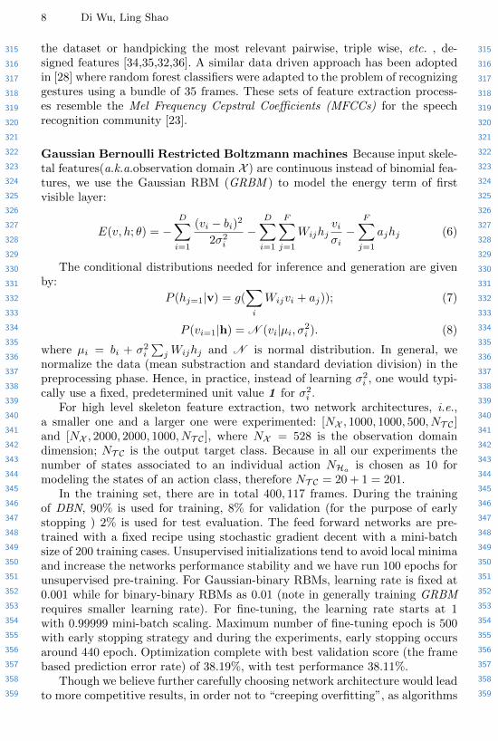
the dataset or handpicking the most relevant pairwise, triple wise, etc. , de-signed features [34,35,32,36]. A similar data driven approach has been adoptedin [28] where random forest classifiers were adapted to the problem of recognizinggestures using a bundle of 35 frames. These sets of feature extraction process-es resemble the Mel Frequency Cepstral Coefficients (MFCCs) for the speechrecognition community [23].
Gaussian Bernoulli Restricted Boltzmann machines Because input skele-tal features(a.k.a.observation domain X ) are continuous instead of binomial fea-tures, we use the Gaussian RBM (GRBM ) to model the energy term of firstvisible layer:
E(v, h; θ) = −D∑i=1
(vi − bi)2
2σ2i
−D∑i=1
F∑j=1
Wijhjviσi−
F∑j=1
ajhj (6)
The conditional distributions needed for inference and generation are givenby:
P (hj=1|v) = g(∑i
Wijvi + aj)); (7)
P (vi=1|h) = N (vi|µi, σ2i ). (8)
where µi = bi + σ2i
∑j Wijhj and N is normal distribution. In general, we
normalize the data (mean substraction and standard deviation division) in thepreprocessing phase. Hence, in practice, instead of learning σ2
i , one would typi-cally use a fixed, predetermined unit value 1 for σ2
i .For high level skeleton feature extraction, two network architectures, i.e.,
a smaller one and a larger one were experimented: [NX , 1000, 1000, 500, NT C ]and [NX , 2000, 2000, 1000, NT C ], where NX = 528 is the observation domaindimension; NT C is the output target class. Because in all our experiments thenumber of states associated to an individual action NHa is chosen as 10 formodeling the states of an action class, therefore NT C = 20 + 1 = 201.
In the training set, there are in total 400, 117 frames. During the trainingof DBN, 90% is used for training, 8% for validation (for the purpose of earlystopping ) 2% is used for test evaluation. The feed forward networks are pre-trained with a fixed recipe using stochastic gradient decent with a mini-batchsize of 200 training cases. Unsupervised initializations tend to avoid local minimaand increase the networks performance stability and we have run 100 epochs forunsupervised pre-training. For Gaussian-binary RBMs, learning rate is fixed at0.001 while for binary-binary RBMs as 0.01 (note in generally training GRBMrequires smaller learning rate). For fine-tuning, the learning rate starts at 1with 0.99999 mini-batch scaling. Maximum number of fine-tuning epoch is 500with early stopping strategy and during the experiments, early stopping occursaround 440 epoch. Optimization complete with best validation score (the framebased prediction error rate) of 38.19%, with test performance 38.11%.
Though we believe further carefully choosing network architecture would leadto more competitive results, in order not to “creeping overfitting”, as algorithms

360
361
362
363
364
365
366
367
368
369
370
371
372
373
374
375
376
377
378
379
380
381
382
383
384
385
386
387
388
389
390
391
392
393
394
395
396
397
398
399
400
401
402
403
404
360
361
362
363
364
365
366
367
368
369
370
371
372
373
374
375
376
377
378
379
380
381
382
383
384
385
386
387
388
389
390
391
392
393
394
395
396
397
398
399
400
401
402
403
404
ECCV
#ECCV
#
Deep Dynamic Neural Networks for Gesture Segmentation and Recognition 9
(a) template image (b) test image(c) template
response
(d) shift-resize im-
age
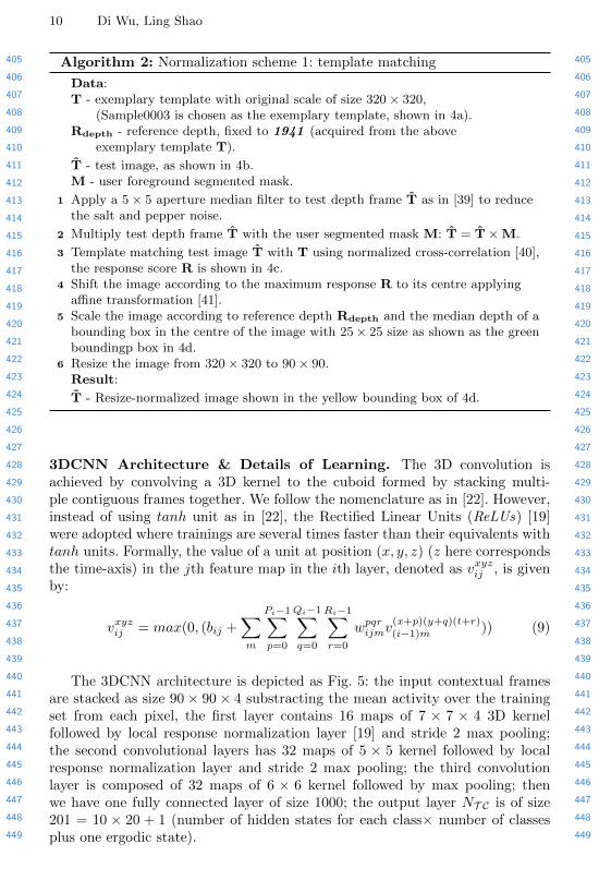
Fig. 4: Illustration of normalization scheme 1: template matching.
over time become too adapted to the dataset, essentially memorizing all itsidiosyncrasies, and losing ability to generalize [37], we would like to treat themodel as the aforementioned more generic approach. Since a completely newapproach will initially have a hard time competing against established, carefullyfine-tuned methods. More fundamentally, it may be that the right way to treatdataset performance numbers is not as a competition for the top place. This way,fundamentally new approaches will not be forced to compete for top performanceright away, but will have a chance to develop and mature.
The performance of skeleton module is shown in Tab 1. And it can be seenthat larger net (Net2) will generally perform better than smaller net (Net1),averaging multi-column nets almost will certainly further improve the perfor-mance [20]. Hence, in the following experiments, only the multi-column averagingresults are reported.
2.6 Depth 3D Module
Preprocessing & Normalizing: shifting, scaling and resizing. Workingdirectly with raw input Kinect recorded data frames, which are 480× 640 pixelimages, can be computationally demanding. Deepmind technology [38] presentedthe first deep learning model to successfully learn control policies directly fromhigh-dimensional sensory input using deep reinforcement learning. Similarly, ba-sic preprocessing steps are adopted aimed at reducing the input dimensionalityfrom the original 480 × 640 pixels to 90 × 90 pixels. The square-sized of thefinal image is required because the used GPU implementation from [19] expectssquare inputs and the input channel should be in the set of [1, 3, 4x]. There aretwo normalization schemes implemented as 2 using depth template matchingmethod and 3 using skeletal joins as assistant normalization. Note that thescheme 2 depends heavily on the provided maximum depth from the recordingscene and scheme 3 depends on the accurate detection of skeleton joins, andboth scheme require the performer remains a roughly static position (thoughthe max pooling scheme in 3DCNN to some extend overcome the problem ofposition shifting). Generally, scheme 3 is more robust than scheme 2 becausethe provided maximum depth can sometimes be very noisy, e.g., Sample0671,Sample0692, Sample0699, etc. After the normalization and resizing, a cuboid of4 frames, hence, size 90× 90× 4, is extracted as a spatio-temporal unit.
405
406
407
408
409
410
411
412
413
414
415
416
417
418
419
420
421
422
423
424
425
426
427
428
429
430
431
432
433
434
435
436
437
438
439
440
441
442
443
444
445
446
447
448
449
405
406
407
408
409
410
411
412
413
414
415
416
417
418
419
420
421
422
423
424
425
426
427
428
429
430
431
432
433
434
435
436
437
438
439
440
441
442
443
444
445
446
447
448
449
ECCV
#ECCV
#
10 Di Wu, Ling Shao
Algorithm 2: Normalization scheme 1: template matching
Data:T - exemplary template with original scale of size 320× 320,
(Sample0003 is chosen as the exemplary template, shown in 4a).Rdepth - reference depth, fixed to 1941 (acquired from the above
exemplary template T).
T - test image, as shown in 4b.M - user foreground segmented mask.
1 Apply a 5× 5 aperture median filter to test depth frame T as in [39] to reducethe salt and pepper noise.
2 Multiply test depth frame T with the user segmented mask M: T = T×M.
3 Template matching test image T with T using normalized cross-correlation [40],the response score R is shown in 4c.
4 Shift the image according to the maximum response R to its centre applyingaffine transformation [41].
5 Scale the image according to reference depth Rdepth and the median depth of abounding box in the centre of the image with 25× 25 size as shown as the greenboundingp box in 4d.
6 Resize the image from 320× 320 to 90× 90.Result:
T - Resize-normalized image shown in the yellow bounding box of 4d.
3DCNN Architecture & Details of Learning. The 3D convolution isachieved by convolving a 3D kernel to the cuboid formed by stacking multi-ple contiguous frames together. We follow the nomenclature as in [22]. However,instead of using tanh unit as in [22], the Rectified Linear Units (ReLUs) [19]were adopted where trainings are several times faster than their equivalents withtanh units. Formally, the value of a unit at position (x, y, z) (z here correspondsthe time-axis) in the jth feature map in the ith layer, denoted as vxyzij , is givenby:
vxyzij = max(0, (bij +∑m
Pi−1∑p=0
Qi−1∑q=0
Ri−1∑r=0
wpqrijmv
(x+p)(y+q)(t+r)(i−1)m )) (9)
The 3DCNN architecture is depicted as Fig. 5: the input contextual framesare stacked as size 90× 90× 4 substracting the mean activity over the trainingset from each pixel, the first layer contains 16 maps of 7 × 7 × 4 3D kernelfollowed by local response normalization layer [19] and stride 2 max pooling;the second convolutional layers has 32 maps of 5 × 5 kernel followed by localresponse normalization layer and stride 2 max pooling; the third convolutionlayer is composed of 32 maps of 6 × 6 kernel followed by max pooling; thenwe have one fully connected layer of size 1000; the output layer NT C is of size201 = 10 × 20 + 1 (number of hidden states for each class× number of classesplus one ergodic state).
450
451
452
453
454
455
456
457
458
459
460
461
462
463
464
465
466
467
468
469
470
471
472
473
474
475
476
477
478
479
480
481
482
483
484
485
486
487
488
489
490
491
492
493
494
450
451
452
453
454
455
456
457
458
459
460
461
462
463
464
465
466
467
468
469
470
471
472
473
474
475
476
477
478
479
480
481
482
483
484
485
486
487
488
489
490
491
492
493
494
ECCV
#ECCV
#
Deep Dynamic Neural Networks for Gesture Segmentation and Recognition 11
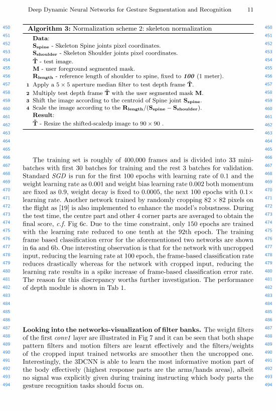
Algorithm 3: Normalization scheme 2: skeleton normalization
Data:Sspine - Skeleton Spine joints pixel coordinates.Sshoulder - Skeleton Shoulder joints pixel coordinates.
T - test image.M - user foreground segmented mask.Rlength - reference length of shoulder to spine, fixed to 100 (1 meter).
1 Apply a 5× 5 aperture median filter to test depth frame T.
2 Multiply test depth frame T with the user segmented mask M.3 Shift the image according to the centroid of Spine joint Sspine.4 Scale the image according to the Rlength/(Sspine − Sshoulder).
Result:
T - Resize the shifted-scaledp image to 90× 90 .
The training set is roughly of 400,000 frames and is divided into 33 mini-batches with first 30 batches for training and the rest 3 batches for validation.Standard SGD is run for the first 100 epochs with learning rate of 0.1 and theweight learning rate as 0.001 and weight bias learning rate 0.002 both momentumare fixed as 0.9, weight decay is fixed to 0.0005, the next 100 epochs with 0.1×learning rate. Another network trained by randomly cropping 82× 82 pixels onthe flight as [19] is also implemented to enhance the model’s robustness. Duringthe test time, the centre part and other 4 corner parts are averaged to obtain thefinal score, c.f. Fig 6c. Due to the time constraint, only 150 epochs are trainedwith the learning rate reduced to one tenth at the 92th epoch. The trainingframe based classification error for the aforementioned two networks are shownin 6a and 6b. One interesting observation is that for the network with uncroppedinput, reducing the learning rate at 100 epoch, the frame-based classification ratereduces drastically whereas for the network with cropped input, reducing thelearning rate results in a spike increase of frame-based classification error rate.The reason for this discrepancy worths further investigation. The performanceof depth module is shown in Tab 1.
Looking into the networks-visualization of filter banks. The weight filtersof the first conv1 layer are illustrated in Fig 7 and it can be seen that both shapepattern filters and motion filters are learnt effectively and the filters/weightsof the cropped input trained networks are smoother then the uncropped one.Interestingly, the 3DCNN is able to learn the most informative motion part ofthe body effectively (highest response parts are the arms/hands areas), albeitno signal was explicitly given during training instructing which body parts thegesture recognition tasks should focus on.

495
496
497
498
499
500
501
502
503
504
505
506
507
508
509
510
511
512
513
514
515
516
517
518
519
520
521
522
523
524
525
526
527
528
529
530
531
532
533
534
535
536
537
538
539
495
496
497
498
499
500
501
502
503
504
505
506
507
508
509
510
511
512
513
514
515
516
517
518
519
520
521
522
523
524
525
526
527
528
529
530
531
532
533
534
535
536
537
538
539
ECCV
#ECCV
#
12 Di Wu, Ling Shao
Fig. 5: An illustration of the architecture of the 3DCNN architecture.
(a) Frame based classifica-tion error with uncroppedinput.
(b) Frame based classifica-tion error with cropped in-put.
(c) Cropped imagesto enhance model’srobustness.
Fig. 6: Visualization of the first filters and training statistics for 3DCNN.
2.7 Post-Processing
The predicted token less than 20 frames are discarded as noisy tokens. Note thatthere are many noisy gesture tokens predicted by viterbi decoding. One way tosift through the noisy tokens is to discard the token path log probability smallthan certain threshold. However, because the metric of this challenge: Jaccardindex strongly penalizes false negatives, experiments show that it’s better tohave more false positives than to miss true positives. Effective ways to detectfalse positives should be an interesting aspect of future works.
2.8 Score Fusion
To fuse the dual model prediction, the strategy shown as Fig 8 is adopted.The complementary properties of both modules can be seen from the Viterbi

540
541
542
543
544
545
546
547
548
549
550
551
552
553
554
555
556
557
558
559
560
561
562
563
564
565
566
567
568
569
570
571
572
573
574
575
576
577
578
579
580
581
582
583
584
540
541
542
543
544
545
546
547
548
549
550
551
552
553
554
555
556
557
558
559
560
561
562
563
564
565
566
567
568
569
570
571
572
573
574
575
576
577
578
579
580
581
582
583
584
ECCV
#ECCV
#
Deep Dynamic Neural Networks for Gesture Segmentation and Recognition 13
Fig. 7: Top left: the conv1 weights of the 3DCNN learnt with uncropped input; top
right: the conv1 weights of the 3DCNN learnt with cropped input. It can be seen that
filters/weights of the cropped input trained networks are smoother. Bottom: visualiza-
tion of sample frames after conv1 layer (Sample0654, 264-296 frames, sampled every
8 frames). It can be seen that the filters of the first convolutional layer are able to
learn both shape pattern(red bounding box) and motion(yellow bounding box). Also
note that the high response maps correspond to the most informative part of the body,
even though during the training process, all local patches are learned indiscriminately
regardless of its location.
path decoding plot in Fig 10. Note that the skeleton module generally performsbetter than the depth module, one reason could be that the skeleton joints learntfrom [25] lie in success of utilizing huge and highly varied training data: fromboth realistic and synthetic depth images, a total number of 1 million imageswere used to train the deep randomized decision forest classifier in order to avoidoverfitting. Hence skeleton data are more robust.
2.9 Computational complexity
Though learning the Deep Neural Networks using stochastic gradient descent istediously lengthy, once the model finishes training, with a low inference cost, ourframework can perform real-time video sequence labeling. Specifically, a singlefeed forward neural network incurs trivial computational time (O(T )) and isfast because it requires only matrix products and convolution operations. Thecomplexity of Viterbi algorithm is O(T ∗ |S|2) with number of frames T andstate number S.

585
586
587
588
589
590
591
592
593
594
595
596
597
598
599
600
601
602
603
604
605
606
607
608
609
610
611
612
613
614
615
616
617
618
619
620
621
622
623
624
625
626
627
628
629
585
586
587
588
589
590
591
592
593
594
595
596
597
598
599
600
601
602
603
604
605
606
607
608
609
610
611
612
613
614
615
616
617
618
619
620
621
622
623
624
625
626
627
628
629
ECCV
#ECCV
#
14 Di Wu, Ling Shao
Fig. 8: Illustration of descriptor fusion.
```````````ModuleEvaluation Set
Validation Test
Skeleton–DBDN Net1 0.7468 -
Skeleton–DBDN Net2 0.8017 -
Skeleton–DBDN MultiNet 0.8236 0.7873
Depth–3DCNN Norm1 2 0.6378 -
Depth–3DCNN Norm2 3 0.6924 0.6371
Score Fusion 0.8045 0.8162
Table 1: Comparison of results in terms of Jaccard index between different network
structures and various modules. DBDN Net1 corresponds to network structure of
[528, 1000, 1000, 500, 201] and DBDN Net2 [528, 2000, 2000, 1000, 201], DBDN Multi-
Net is the average of 3 Nets (2 Net1 and 1 Net2 with different initializations). It can be
seen that larger net has better performance and multi-column net will further improve
the classification rate. Norm1 corresponds to the normalization scheme 2 and Norm2
corresponds to the scheme 3.
3 Conclusion and Discussion
Hand-engineered, task-specific features are often less adaptive and time-consumingto design. This difficulty is more pronounced with multimodal data as the fea-tures have to relate multiple data sources. In this paper, we presented a novelDeep Dynamic Neural Networks(DDNN) framework that utilizes Deep BeliefNetworks and 3D Convolutional Neural Networks for learning contextual frame-level representations and modeling emission probabilities for Markov Field. Theheterogeneous inputs from skeletal joints and depth images require different fea-ture learning methods and the late fusion scheme is adopted at the score level.The experimental results on bi-modal time series data show that the multimodalDDNN framework can learn a good model of the joint space of multiple sensoryinputs, and is consistently as good as/better than the unimodal input, openingthe door for exploring the complementary representation among multimodal in-puts. It also suggests that learning features directly from data is a very importantresearch direction and with more and more data and flops-free computationalpower, the learning-based methods are not only more generalizable to many do-mains, but also are powerful in combining with other well-studied probabilisticgraphical models for modeling and reasoning dynamic sequences. Future worksinclude learning the share representation amongst the heterogeneous inputs at

630
631
632
633
634
635
636
637
638
639
640
641
642
643
644
645
646
647
648
649
650
651
652
653
654
655
656
657
658
659
660
661
662
663
664
665
666
667
668
669
670
671
672
673
674
630
631
632
633
634
635
636
637
638
639
640
641
642
643
644
645
646
647
648
649
650
651
652
653
654
655
656
657
658
659
660
661
662
663
664
665
666
667
668
669
670
671
672
673
674
ECCV#
ECCV#
Deep Dynamic Neural Networks for Gesture Segmentation and Recognition 15
the penultimate layer and backpropagating the gradient in the share space in aunified representation.
References
1. Escalera, S., Bar, X., Gonzlez, J., Bautista, M., Madadi, M., Reyes, M., Ponce, V.,Escalante, H., Shotton, J., Guyon, I.: Chalearn looking at people challenge 2014:Dataset and results. In: European Conference on Computer Vision workshop.(2014)
2. Liu, L., Shao, L., Zheng, F., Li, X.: Realistic action recognitionvia sparsely-constructed gaussian processes. Pattern Recognition, doi:10.1016/j.patcog.2014.07.006. (2014)
3. Shao, L., Zhen, X., Li, X.: Spatio-temporal laplacian pyramid coding for actionrecognition. IEEE Transactions on Cybernetics, vol. 44, no. 6, pp. 817-827 (2014)
4. Wu, D., Shao, L.: Silhouette analysis-based action recognition via exploiting humanposes. IEEE Transactions on Circuits and Systems for Video Technology, vol. 23,no. 2, pp. 236-243 (2013)
5. Laptev, I.: On space-time interest points. International Journal of ComputerVision (2005)
6. Dollar, P., Rabaud, V., Cottrell, G., Belongie, S.: Behavior recognition via sparsespatio-temporal features. In: Visual Surveillance and Performance Evaluation ofTracking and Surveillance, IEEE (2005)
7. Willems, G., Tuytelaars, T., Gool, L.V.: An efficient dense and scale-invariantspatio-temporal interest point detector. In: European Conference on ComputerVision, Springer (2008)
8. Scovanner, P., Ali, S., Shah, M.: A 3-dimensional sift descriptor and its applicationto action recognition. In: International Conference on Multimedia, ACM (2007)
9. Klaser, A., Marszalek, M., Schmid, C.: A Spatio-Temporal Descriptor Based on3D-Gradients. In: British Machine Vision Conference. (2008)
10. Wang, H., Klaser, A., Schmid, C., Liu, C.L.: Dense trajectories and motion bound-ary descriptors for action recognition. International Journal of Computer Vision(2013)
11. Zhou, T., Tao, D.: Double shrinking sparse dimension reduction. IEEE Transac-tions on Image Processing 22(1): 244-257 (2013)
12. Xu, C., Tao, D.: Large-margin multi-view information bottleneck. IEEE Trans.Pattern Anal. Mach. Intell. 36(8): 1559-1572 (2014)
13. Wang, H., Ullah, M.M., Klaser, A., Laptev, I., Schmid, C., et al.: Evaluation oflocal spatio-temporal features for action recognition. In: British Machine VisionConference. (2009)
14. Taylor, G.W., Fergus, R., LeCun, Y., Bregler, C.: Convolutional learning of spatio-temporal features. In: European Conference on Computer Vision. Springer (2010)
15. Le, Q.V., Zou, W.Y., Yeung, S.Y., Ng, A.Y.: Learning hierarchical invariant spatio-temporal features for action recognition with independent subspace analysis. In:IEEE Conference on Computer Vision and Pattern Recognition. (2011)
16. Baccouche, M., Mamalet, F., Wolf, C., Garcia, C., Baskurt, A.: Spatio-temporalconvolutional sparse auto-encoder for sequence classification. In: British MachineVision Conference. (2012)
17. Hinton, G.E., Osindero, S., Teh, Y.W.: A fast learning algorithm for deep beliefnets. Neural computation (2006)

675
676
677
678
679
680
681
682
683
684
685
686
687
688
689
690
691
692
693
694
695
696
697
698
699
700
701
702
703
704
705
706
707
708
709
710
711
712
713
714
715
716
717
718
719
675
676
677
678
679
680
681
682
683
684
685
686
687
688
689
690
691
692
693
694
695
696
697
698
699
700
701
702
703
704
705
706
707
708
709
710
711
712
713
714
715
716
717
718
719
ECCV#
ECCV#
16 Di Wu, Ling Shao
18. Schmidhuber, J.: Deep learning in neural networks: An overview. arXiv preprintarXiv:1404.7828 (2014)
19. Krizhevsky, A., Sutskever, I., Hinton, G.E.: Imagenet classification with deepconvolutional neural networks. In: Neural Information Processing Systems. (2012)
20. Ciresan, D., Meier, U., Schmidhuber, J.: Multi-column deep neural networks forimage classification. In: IEEE Conference on Computer Vision and Pattern Recog-nition. (2012)
21. Shuiwang Ji, Wei Xu, M.Y., Yu, K.: 3d convolutional neural networks for humanaction recognition. In: International Conference on Machine Learning, IEEE (2010)
22. Ji, S., Xu, W., Yang, M., Yu, K.: 3d convolutional neural networks for humanaction recognition. Pattern Analysis and Machine Intelligence, IEEE Transactionson (2013)
23. Mohamed, A., Dahl, G.E., Hinton, G.: Acoustic modeling using deep belief net-works. Audio, Speech, and Language Processing, IEEE Transactions on (2012)
24. Wu, D., Shao, L.: Leveraging hierarchical parametric networks for skeletal jointsbased action segmentation and recognition. In: IEEE Conference on ComputerVision and Pattern Recognition. (2014)
25. Shotton, J., Fitzgibbon, A., Cook, M., Sharp, T., Finocchio, M., Moore, R., Kip-man, A., Blake, A.: Real-time human pose recognition in parts from single depthimages. In: IEEE Conference on Computer Vision and Pattern Recognition. (2011)
26. Han, J., Shao, L., Shotton, J.: Enhanced computer vision with microsoft kinectsensor: A review. IEEE Transactions on Cybernetics, vol. 43, no. 5, pp. 1317-1333(2013)
27. Escalera, S., Gonzlez, J., Bar, X., Reyes, M., Lops, O., Guyon, I., Athitsos, V.,Escalante, H.J.: Multi-modal gesture recognition challenge 2013: Dataset and re-sults. In: ACM ChaLearn Multi-Modal Gesture Recognition Grand Challenge andWorkshop. (2013)
28. Fothergill, S., Mentis, H.M., Kohli, P., Nowozin, S.: Instructing people for traininggestural interactive systems. In: ACM Computer Human Interaction. (2012)
29. Guyon, I., Athitsos, V., Jangyodsuk, P., Hamner, B., Escalante, H.J.: Chalearngesture challenge: Design and first results. In: IEEE Conference on ComputerVision and Pattern Recognition Workshops. (2012)
30. Wang, J., Liu, Z., Wu, Y., Yuan, J.: Mining actionlet ensemble for action recogni-tion with depth cameras. In: IEEE Conference on Computer Vision and PatternRecognition. (2012)
31. Lehrmann, A., Gehler, P., Nowozin, S.: A non-parametric bayesian network priorof human pose. In: International Conference on Computer Vision. (2013)
32. Nowozin, S., Shotton, J.: Action points: A representation for low-latency onlinehuman action recognition. Technical report (2012)
33. Bishop, C.: Pattern recognition and machine learning. Springer (2006)34. Chaudhry, R., Ofli, F., Kurillo, G., Bajcsy, R., Vidal, R.: Bio-inspired dynamic 3d
discriminative skeletal features for human action recognition. In: IEEE Conferenceon Computer Vision and Pattern Recognition Workshops. (2013)
35. Muller, M., Roder, T.: Motion templates for automatic classification and retrievalof motion capture data. In: SIGGRAPH/Eurographics symposium on Computeranimation, Eurographics Association (2006)
36. Ofli, F., Chaudhry, R., Kurillo, G., Vidal, R., Bajcsy, R.: Sequence of the most in-formative joints (smij): A new representation for human skeletal action recognition.Journal of Visual Communication and Image Representation (2013)
37. Torralba, A., Efros, A.A.: Unbiased look at dataset bias. In: IEEE Conference onComputer Vision and Pattern Recognition. (2011)

720
721
722
723
724
725
726
727
728
729
730
731
732
733
734
735
736
737
738
739
740
741
742
743
744
745
746
747
748
749
750
751
752
753
754
755
756
757
758
759
760
761
762
763
764
720
721
722
723
724
725
726
727
728
729
730
731
732
733
734
735
736
737
738
739
740
741
742
743
744
745
746
747
748
749
750
751
752
753
754
755
756
757
758
759
760
761
762
763
764
ECCV
#ECCV
#
Deep Dynamic Neural Networks for Gesture Segmentation and Recognition 17
38. Mnih, V., Kavukcuoglu, K., Silver, D., Graves, A., Antonoglou, I., Wierstra, D.,Riedmiller, M.: Playing atari with deep reinforcement learning. arXiv preprintarXiv:1312.5602 (2013)
39. Wu, D., Zhu, F., Shao, L.: One shot learning gesture recognition from rgbd im-ages. In: International Conference on Computer Vision and Pattern RecognitionWorkshops. (2012)
40. Lewis, J.: Fast normalized cross-correlation. In: Vision interface. Volume 10. (1995)120–123
41. Bradski, G. Dr. Dobb’s Journal of Software Tools42. Bergstra, J., Breuleux, O., Bastien, F., Lamblin, P., Pascanu, R., Desjardins, G.,
Turian, J., Warde-Farley, D., Bengio, Y.: Theano: a CPU and GPU math expres-sion compiler. In: Proceedings of the Python for Scientific Computing Conference(SciPy). (2010)
4 Supplementary materials
4.1 Deep Learning Library: Theano & cuda-convnet
Theano. The Deep Belief Network library used in this section is Theano [42]2 which is a Python library that allows you to define, optimize, and eval-uate mathematical expressions involving multi-dimensional arrays efficiently.
cuda-convnet. The GPU enabled blazing fast Convolutional Neural Networklibrary used in this section is cuda-convnet [19] 3 which is a fast C++/CUDAimplementation of convolutional (or more generally, feed-forward) neuralnetworks. It can model arbitrary layer connectivity and network depth. Anydirected acyclic graph of layers will do. Training is done using the back-propagation algorithm.
4.2 Details of the Code
Deep Belief Dynamic Networks The python project for “Leveraging Hierar-chical Parametric Network for Skeletal Joints Action Segmentation and Recog-nition” can be found at:https://github.com/stevenwudi/CVPR_2014_code
Deep 3D Convolutional Dynamic Networks The python project, C++/CUDAbackend for Deep 3D Convolutional Dynamic Network can be found at:https://github.com/stevenwudi/3DCNN_HMM
4.3 Extra Figures for Illustration
2 http://deeplearning.net/software/theano/3 https://code.google.com/p/cuda-convnet/

765
766
767
768
769
770
771
772
773
774
775
776
777
778
779
780
781
782
783
784
785
786
787
788
789
790
791
792
793
794
795
796
797
798
799
800
801
802
803
804
805
806
807
808
809
765
766
767
768
769
770
771
772
773
774
775
776
777
778
779
780
781
782
783
784
785
786
787
788
789
790
791
792
793
794
795
796
797
798
799
800
801
802
803
804
805
806
807
808
809
ECCV
#ECCV
#
18 Di Wu, Ling Shao
Fig. 9: More illustrations of the middle level features from the activation images after
first convolutional layer. High response arms and hands areas are learnt automatically
without explicit learning signal in term of location information.
Fig. 10: Viterbi decoding of two modules and their fusion result of sample sequence
704. Top to bottom: skeleton, depth, score fusion with x-axis representing the time and
y-axis representing the hidden states of all the classes with the ergodic state at the
bottom. Red lines are the ground truth label, cyan lines are the viterbi shortest path
and yellow lines are the predicted label. There are some complementary information
of the two modules and generally skeletal module outperforms the depth module. The
fusion of the two could exploit the uncertainty, e.g. light green dashed box indicates
that depth module makes the correct prediction whereas the skeletal module fails, the
combined module is still making the correct prediction.
810
811
812
813
814
815
816
817
818
819
820
821
822
823
824
825
826
827
828
829
830
831
832
833
834
835
836
837
838
839
840
841
842
843
844
845
846
847
848
849
850
851
852
853
854
810
811
812
813
814
815
816
817
818
819
820
821
822
823
824
825
826
827
828
829
830
831
832
833
834
835
836
837
838
839
840
841
842
843
844
845
846
847
848
849
850
851
852
853
854
ECCV
#ECCV
#
Deep Dynamic Neural Networks for Gesture Segmentation and Recognition 19
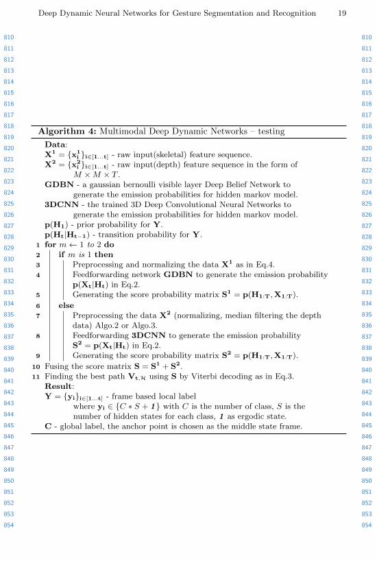
Algorithm 4: Multimodal Deep Dynamic Networks – testing
Data:X1 = {x1
i }i∈[1...t] - raw input(skeletal) feature sequence.X2 = {x2
i }i∈[1...t] - raw input(depth) feature sequence in the form ofM ×M × T .
GDBN - a gaussian bernoulli visible layer Deep Belief Network togenerate the emission probabilities for hidden markov model.
3DCNN - the trained 3D Deep Convolutional Neural Networks togenerate the emission probabilities for hidden markov model.
p(H1) - prior probability for Y.p(Ht|Ht−1) - transition probability for Y.
1 for m← 1 to 2 do2 if m is 1 then3 Preprocessing and normalizing the data X1 as in Eq.4.4 Feedforwarding network GDBN to generate the emission probability
p(Xt|Ht) in Eq.2.5 Generating the score probability matrix S1 = p(H1:T,X1:T).
6 else7 Preprocessing the data X2 (normalizing, median filtering the depth
data) Algo.2 or Algo.3.8 Feedforwarding 3DCNN to generate the emission probability
S2 = p(Xt|Ht) in Eq.2.9 Generating the score probability matrix S2 = p(H1:T,X1:T).
10 Fusing the score matrix S = S1 + S2.11 Finding the best path Vt,H using S by Viterbi decoding as in Eq.3.
Result:Y = {yi}i∈[1...t] - frame based local label
where yi ∈ {C ∗ S + 1} with C is the number of class, S is thenumber of hidden states for each class, 1 as ergodic state.
C - global label, the anchor point is chosen as the middle state frame.