ECE 6310Spring 2012Assignment 4 Solutions

Balanis 7.13

The far-field approximation replaces the distance from the source point to the observation point by the distance from the source point to a plane containing to the observation point (where the plane is perpendicular to the observation point vector, r.)

R ≈ r − r ⋅ ′r

The approximation is used in the phase factors, so that the array factor, which adds up the complex contribution of the various array elements, can be written as

F θ,φ( ) = ane− jβ r ⋅ ′rn

n=0

N −1

∑

where the common phase factor due to r has been dropped, since the absolute phase is not important. For the geometry of the set of images, see the demonstration and ray tracing figure in the resources section of the class website. The equivalent set of sources are arranged in a polygon around the origin.

′rn = xscos nα( ) + yssin nα( ) N =2πα

The observation point unit vector in spherical coordinates is

r = xsinθ cosφ + ysinθ sinφ + z cosθ

The array factor them becomes

F θ,φ( ) = −1( )n e− jβs sinθ cos nα( ) cosφ+sin nα( )sinφ⎡⎣ ⎤⎦

n=0

N −1

∑ N even

where the sign of the array factor terms alternates around the polygon. (Recall the sign of the image required for parallel electric dipoles above a PEC.) The angles that lead to odd vertex polygons do not work out since the sign cannot alternate consistently around the polygon. Some images land on a reflecting plane and thus have zero amplitude.

When the include angle α is 60 degrees we have a hexagon.

cos nα( ) = 1, 12, − 12, −1, − 1

2, 12

⎛⎝⎜

⎞⎠⎟

sin nα( ) = 0, 32, 32, 0, − 3

2, − 3

2⎛

⎝⎜⎞

⎠⎟

and the six-term array factor is

F θ,φ( ) = e− jβs sinθ cosφ[ ] − e− j 12βs sinθ cosφ+ 3 sinφ⎡⎣ ⎤⎦ + e

− j 12βs sinθ − cosφ+ 3 sinφ⎡⎣ ⎤⎦ − e− jβs sinθ − cosφ[ ] + e

− j 12βs sinθ − cosφ− 3 sinφ⎡⎣ ⎤⎦ − e

− j 12βs sinθ cosφ− 3 sinφ⎡⎣ ⎤⎦

The exponentials can be combined into trigonometric functions

F θ,φ( ) = −2 j sin βssinθ cosφ[ ] + 2 j sin 12βssinθ cosφ + 3sinφ( )⎡

⎣⎢⎤⎦⎥+ 2 j sin 1

2βssinθ cosφ − 3sinφ( )⎡

⎣⎢⎤⎦⎥

Making a substitution with the dimensionless variables

X = βssinθ cosφY = βssinθ sinφ

and dropping a common phase factor yields

F θ,φ( ) = 2sin X − 2sin X2+ 3Y

2⎛⎝⎜

⎞⎠⎟− 2sin X

2− 3Y

2⎛⎝⎜

⎞⎠⎟

Then using the trigonometric identities

sin2a = 2sinacosasin a + b( ) + sin a − b( ) = 2sinacosb

gives

F θ,φ( ) = 4sin X2

⎛⎝⎜

⎞⎠⎟cos X

2⎛⎝⎜

⎞⎠⎟− 4sin X

2⎛⎝⎜

⎞⎠⎟cos 3Y

2⎛⎝⎜

⎞⎠⎟

and finally, factoring, we have the desired result.

F θ,φ( ) = 4sin X2

⎛⎝⎜

⎞⎠⎟cos X

2⎛⎝⎜

⎞⎠⎟− cos 3Y

2⎛⎝⎜

⎞⎠⎟

⎡⎣⎢

⎤⎦⎥

When the include angle α is 45 degrees we have an octagon.

cos nα( ) = 1, 12, 0, − 1

2, −1, − 1

2, 0, 1

2⎛⎝⎜

⎞⎠⎟

sin nα( ) = 0, 12, 1, 1

2, 0, − 1

2, −1, − 1

2⎛⎝⎜

⎞⎠⎟

and an eight-term array factor

F θ,φ( ) = e− jβs sinθ cosφ[ ] − e−12jβs sinθ cosφ+sinφ[ ]

+ e− jβs sinθ sinφ[ ] − e−12jβs sinθ − cosφ+sinφ[ ]

+ e− jβs sinθ − cosφ[ ] − e−12jβs sinθ − cosφ−sinφ[ ]

+ e− jβs sinθ − sinφ[ ] − e−12jβs sinθ cosφ−sinφ[ ]

Combine into trigonometric functions.

F θ,φ( ) = 2cos βssinθ cosφ[ ]− 2cos 12βssinθ cosφ + sinφ( )⎡

⎣⎢⎤⎦⎥+ 2cos βssinθ sinφ[ ]− 2cos 1

2βssinθ cosφ − sinφ( )⎡

⎣⎢⎤⎦⎥

Perform the substitutions.

F θ,φ( ) = 2cosX − 2cos X2+Y2

⎛⎝⎜

⎞⎠⎟+ 2cosY − 2cos X

2−Y2

⎛⎝⎜

⎞⎠⎟

Apply the trigonometric identity

cos a + b( ) + cos a − b( ) = 2cosacosb

to obtain

F θ,φ( ) = 2 cos X( ) + cos Y( ) − 2cos X2

⎛⎝⎜

⎞⎠⎟cos X

2⎛⎝⎜

⎞⎠⎟

⎡

⎣⎢

⎤

⎦⎥

When the include angle α is 30 degrees we have a dodecagon.

cos nα( ) = 1, 32, 12, 0, − 1

2, − 3

2, −1, − 3

2−12, 0, 1

2, 32

⎛

⎝⎜⎞

⎠⎟

sin nα( ) = 0, 12, 32, 1, 3

2, 12, 0, − 1

2,− 3

2, −1, − 3

2, − 12

⎛

⎝⎜⎞

⎠⎟

and a twelve term array factor.

F θ,φ( ) = e− jβs sinθ cosφ[ ] − e− jβs sinθ 3

2cosφ+ 1

2sinφ

⎡

⎣⎢

⎤

⎦⎥+ e

− jβs sinθ 12cosφ+ 3

2sinφ

⎡

⎣⎢

⎤

⎦⎥− e− jβs sinθ sinφ[ ] + e

− jβs sinθ −12cosφ+ 3

2sinφ

⎡

⎣⎢

⎤

⎦⎥− e

− jβs sinθ −32cosφ+ 1

2sinφ

⎡

⎣⎢

⎤

⎦⎥

+ e− jβs sinθ − cosφ[ ] − e− jβs sinθ −

32cosφ− 1

2sinφ

⎡

⎣⎢

⎤

⎦⎥+ e

− jβs sinθ −12cosφ− 3

2sinφ

⎡

⎣⎢

⎤

⎦⎥− e− jβs sinθ − sinφ[ ] + e

− jβs sinθ 12cosφ− 3

2sinφ

⎡

⎣⎢

⎤

⎦⎥− e

− jβs sinθ 32cosφ− 1

2sinφ

⎡

⎣⎢

⎤

⎦⎥

F θ,φ( ) = 2cos βssinθ cosφ[ ]− 2cos βssinθ 32cosφ +

12sinφ

⎛

⎝⎜⎞

⎠⎟⎡

⎣⎢⎢

⎤

⎦⎥⎥+ 2cos βssinθ 1

2cosφ +

32sinφ

⎛

⎝⎜⎞

⎠⎟⎡

⎣⎢⎢

⎤

⎦⎥⎥− 2cos βssinθ sinφ[ ] + 2cos βssinθ 1

2cosφ −

32sinφ

⎛

⎝⎜⎞

⎠⎟⎡

⎣⎢⎢

⎤

⎦⎥⎥− 2cos βssinθ 3

2cosφ −

12sinφ

⎛

⎝⎜⎞

⎠⎟⎡

⎣⎢⎢

⎤

⎦⎥⎥

Combine into trigonometric functions.

F θ,φ( ) = 2cos X( ) − 2cos 32X +

12Y

⎛

⎝⎜⎞

⎠⎟+ 2cos 1

2X +

32Y

⎛

⎝⎜⎞

⎠⎟− 2cos Y( ) + 2cos 1

2X −

32Y

⎛

⎝⎜⎞

⎠⎟− 2cos 3

2X −

12Y

⎛

⎝⎜⎞

⎠⎟

Apply the trigonometric identity above.

F θ,φ( ) = 2 cos X( ) − cos Y( ) − 2cos 3 X2

⎛⎝⎜

⎞⎠⎟cos Y

2⎛⎝⎜

⎞⎠⎟+ 2cos X

2⎛⎝⎜

⎞⎠⎟cos 3Y

2⎛⎝⎜

⎞⎠⎟

⎡⎣⎢

⎤⎦⎥

Balanis 7.17

(a) An electric current loop gives fields approximately the same as a pair of separated magnetic charges with opposite sign, i.e. a magnetic dipole. The image of a magnetic charge in a perfect magnetic conductor (PMC) is a magnetic charge of opposite sign and equal distance below the plane of the PMC. Thus the images of magnetic dipole charges have opposite sign, but also opposite relative position. Thus the magnetic dipole image has the same magnitude and orientation as the magnetic dipole itself. Thus the image of an electric current loop has the same magnitude and phase as the actual loop,

(b) and thus the direction of current must be CCW as in the actual loop.

Balanis 7.43

Just as in Example 7-3, the equivalent problem has surface currents in free space

Ms = −2n × Ea

Js = 0

With the given aperture field

Ea =ρE0J1

′χ11a

ρ⎛⎝⎜

⎞⎠⎟sinφρ

+ φE0 ′J1′χ11a

ρ⎛⎝⎜

⎞⎠⎟cosφ ρ ≤ a

0 ρ > a

⎧

⎨⎪

⎩⎪

and using the right-hand relationship for the cylindrical coordinate unit vectors

z × ρ = φ

z × φ = −ρ

we find

Ms = 2−φE0J1

′χ11a

ρ⎛⎝⎜

⎞⎠⎟sinφρ

+ ρE0 ′J1′χ11a

ρ⎛⎝⎜

⎞⎠⎟cosφ ρ ≤ a

0 ρ > a

⎧

⎨⎪

⎩⎪

Balanis 8.2

(a) The cut-off frequency, equation 8-16, can be written in terms of relative material properties and speed of light in vacuum.

fc( )mn =1

2π εµmπa

⎛⎝⎜

⎞⎠⎟2

+nπb

⎛⎝⎜

⎞⎠⎟2

=c

2π εrµr

mπa

⎛⎝⎜

⎞⎠⎟2

+nπb

⎛⎝⎜

⎞⎠⎟2

For this guide the lowest order mode, TE10, the cut-off is

a = 2.286 cmεr = 2.56µr = 1c = 2.9979 ×108 m/sfc( )10 4.10 GHz

(b) The guide wavelength

λz =λ

1− fcf

⎛⎝⎜

⎞⎠⎟

2

is given in terms of the wavelength in the medium

λ =vf=

cf εrµr

with value

λz 2.05 cm

(c) The wave impedance

Zw =η

1− fcf

⎛⎝⎜

⎞⎠⎟

2

is given in terms of the medium impedance

η = η0µr

εr

with value

η0 376.73 ΩZw = 258.1 Ω

(d) The phase velocity

vp =v

1− fcf

⎛⎝⎜

⎞⎠⎟

2

is given in terms of the medium velocity

v = cεrµr

with value

vp 2.05 ×108 m/s

(e) The group velocity is inversely related to the phase velocity.

vg =

v2

vp 1.71×108 m/s

Balanis 8.12

Start with the TE modes. A form for the general solution for the electric vector potential for waves traveling in the positive z-direction.

Fz+ x, y, z( ) = C1 cos βxx( ) + D1 sin βxx( )⎡⎣ ⎤⎦ C2 cos βyy( ) + D2 sin βyy( )⎡⎣ ⎤⎦e

− jβz z

The electric field is found from the definition of electric vector potential, and the magnetic field from the electric field, using Maxwell’s equations. See equation 8-1. First we find two field components necessary for enforcing the boundary conditions.

Ex = −1ε∂Fz∂y

= −βy

εC1 cos βxx( ) + D1 sin βxx( )⎡⎣ ⎤⎦ −C2 sin βyy( ) + D2 cos βyy( )⎡⎣ ⎤⎦e

− jβz z

Hy = − j 1ωεµ

∂2Fz∂y∂z

= −βyβz

ωεµC1 cos βxx( ) + D1 sin βxx( )⎡⎣ ⎤⎦ −C2 sin βyy( ) + D2 cos βyy( )⎡⎣ ⎤⎦e

− jβz z

The boundary conditions require tangential components of the electric field to be zero on the horizontal boundaries and tangential components of the magnetic field to be zero on the vertical boundaries.

Ex x,0, z( ) = Ex x,b, z( ) = 0Hy 0, y, z( ) = Hy a, y, z( ) = 0Hz 0, y, z( ) = Hz a, y, z( ) = 0

Enforcing the condition on the x-component of the electric field

Ex x,0, z( ) = −βy

εC1 cos βxx( ) + D1 sin βxx( )⎡⎣ ⎤⎦ D2[ ]e− jβz z = 0 ⇒ D2 = 0

Ex x,b, z( ) = −βy

εC1 cos βxx( ) + D1 sin βxx( )⎡⎣ ⎤⎦ sin βyb( )⎡⎣ ⎤⎦e

− jβz z = 0 ⇒ sin βyb( ) = 0 ⇒ βy =nπb

we find the D2 is zero and βy must have a discrete set of values. Enforcing the condition on the y-component of the magnetic field

Hy 0, y, z( ) = −βyβz

ωεµC1[ ] sin βyy( )⎡⎣ ⎤⎦e

− jβz z = 0 ⇒ C1 = 0

Hy a, y, z( ) = −βyβz

ωεµsin βxa( )⎡⎣ ⎤⎦ sin βyy( )⎡⎣ ⎤⎦e

− jβz z = 0 ⇒ sin βxa( ) = 0 ⇒ βx =mπa

we find that C1 is zero and βx must have a discrete set of values. One can check that the condition on the z-component of the magnetic field does not add any further constraint on the general solution. The electric vector potential with the remaining terms is.

Fz+ x, y, z( ) = sin βxx( )cos βyy( )e− jβz z

From equation 8-1 the complete set of fields is

Ex =βy

εsin βxx( )sin βyy( )e− jβz z Hx = −

βxβz

ωεµcos βxx( )cos βyy( )e− jβz z

Ey =βx

εcos βxx( )cos βyy( )e− jβz z Hy =

βyβz

ωεµsin βxx( )sin βyy( )e− jβz z

Ez = 0 Hz = − j βc2

ωεµsin βxx( )cos βyy( )e− jβz z

βx =mπa

βy =nπb

m = 1,2,3,... n = 0,1,2,3,...

with the eigenvalues (βx and βy) given as shown. The mode for m = 0 has zero field and is omitted. I have left off an overall scaling factor as Balanis uses.

For the TM modes, a form for the general solution for the magnetic vector potential for waves traveling in the positive z-direction.

Az+ x, y, z( ) = C1 cos βxx( ) + D1 sin βxx( )⎡⎣ ⎤⎦ C2 cos βyy( ) + D2 sin βyy( )⎡⎣ ⎤⎦e

− jβz z

As above, we first find the two field components necessary for enforcing the boundary conditions.

Ex = − j 1ωεµ

∂2Az∂x∂z

= −βxβz

ωεµ−C1 sin βxx( ) + D1 cos βxx( )⎡⎣ ⎤⎦ C2 cos βyy( ) + D2 sin βyy( )⎡⎣ ⎤⎦e

− jβz z

Hy = −1µ∂Az∂x

= −βx

µ−C1 sin βxx( ) + D1 cos βxx( )⎡⎣ ⎤⎦ C2 cos βyy( ) + D2 sin βyy( )⎡⎣ ⎤⎦e

− jβz z

Enforcing the condition on the y-component of the magnetic field

Hy 0, y, z( ) = −βx

µD1[ ] C2 cos βyy( ) + D2 sin βyy( )⎡⎣ ⎤⎦e

− jβz z = 0 ⇒ D1 = 0

Hy a, y, z( ) = −βx

µsin βxa( )⎡⎣ ⎤⎦ C2 cos βyy( ) + D2 sin βyy( )⎡⎣ ⎤⎦e

− jβz z = 0 ⇒ sin βxa( ) = 0 ⇒ βx =mπa

we find that D1 is zero and βx must have a discrete set of values. Enforcing the condition on the y-component of the magnetic field

Ex x,0, z( ) = −βxβz

ωεµsin βxx( )⎡⎣ ⎤⎦ C2[ ]e− jβz z = 0 ⇒ C2 = 0

Ex x,b, z( ) = −βxβz

ωεµsin βxx( )⎡⎣ ⎤⎦ sin βyb( )⎡⎣ ⎤⎦e

− jβz z = 0 ⇒ sin βyb( ) = 0 ⇒ βy =nπb

we find the C2 is zero and βy must have a discrete set of values. As above, the condition on the z-component of the magnetic field does not add any further constraint on the general solution. The magnetic vector potential with the remaining terms is.

Az+ x, y, z( ) = cos βxx( )sin βyy( )e− jβz z

From equation 8-1 the complete set of fields is

Ex =βxβz

ωεµsin βxx( )sin βyy( )e− jβz z Hx =

βy

µcos βxx( )cos βyy( )e− jβz z

Ey = −βyβz

ωεµcos βxx( )cos βyy( )e− jβz z Hy =

βx

µsin βxx( )sin βyy( )e− jβz z

Ez = − j βc2

ωεµcos βxx( )sin βyy( )e− jβz z Hz = 0

βx =mπa

βy =nπb

m = 0,1,2,3,... n = 1,2,3,...

with the eigenvalues (βx and βy) given as shown. The mode for n = 0 has zero field and is omitted.

The cutoff frequency expression is the same as for standard (all PEC walled) waveguides since it just depends on the transverse components of β, which are the same as the in that case.

fc( )mn =1

2π εµmπa

⎛⎝⎜

⎞⎠⎟2

+nπb

⎛⎝⎜

⎞⎠⎟2

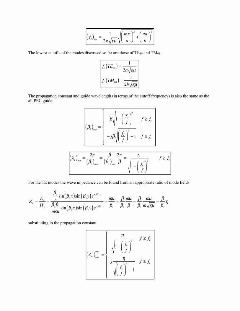
The lowest cutoffs of the modes discussed so far are those of TE10 and TM01.

fc TE10( ) = 12a εµ

fc TM 01( ) = 12b εµ

The propagation constant and guide wavelength (in terms of the cutoff frequency) is also the same as the all PEC guide.

βz( )mn =β 1− fc

f⎛⎝⎜

⎞⎠⎟

2

f ≥ fc

− jβ fcf

⎛⎝⎜

⎞⎠⎟

2

−1 f ≤ fc

⎧

⎨

⎪⎪⎪

⎩

⎪⎪⎪

λz( )mn =2πβz( )mn

=β

βz( )mn2πβ

=λ

1− fcf

⎛⎝⎜

⎞⎠⎟

2f ≥ fc

For the TE modes the wave impedance can be found from an appropriate ratio of mode fields

Zw =Ex

Hy

=

βy

εsin βxx( )sin βyy( )e− jβz z

βyβz

ωεµsin βxx( )sin βyy( )e− jβz z

=ωµβz

=ββz

ωµβ

=ββz

ωµω εµ

=ββz

η

substituting in the propagation constant

Zw( )mnTEz =

η

1− fcf

⎛⎝⎜

⎞⎠⎟

2f ≥ fc

j η

fcf

⎛⎝⎜

⎞⎠⎟

2

−1

f ≤ fc

⎧

⎨

⎪⎪⎪⎪

⎩

⎪⎪⎪⎪

which again is the same as the all PEC guide. For TM modes we have

Zw =Ex

Hy

=

βxβz

ωεµsin βxx( )sin βyy( )e− jβz z

βx

µsin βxx( )sin βyy( )e− jβz z

=βz

ωε=βz

ββωε

=βz

βω εµωε

=βz

βη

Zw( )mnTM z

=

η 1− fcf

⎛⎝⎜

⎞⎠⎟

2

f ≥ fc

− jη fcf

⎛⎝⎜

⎞⎠⎟

2

−1 f ≤ fc

⎧

⎨

⎪⎪⎪

⎩

⎪⎪⎪

While all the modes discussed above are valid, none of them is the dominant mode (i.e. has the lowest cutoff). The procedure above misses the fact that a simple plane wave also satisfies the boundary conditions as can be seen by inspection. This mode is not cutoff and has the properties of the medium. If you missed this mode, note that the Balanis solutions manual also missed it.

E = yE0e− jβz

H = −x E0ηe− jβz

fc = 0 βz = β λz = λ Zw = η

This TEM waveguide is frequently used in simulations where one wants to see the response to a plane wave.