ECE 720T5 Fall 2011 Cyber-Physical Systems

Rodolfo Pellizzoni

2 / 47

Topic Today: End-To-End Analysis• HW platform comprises multiple resources

– Processing Elements– Communication Links

• SW model consists of multiple independent flows or transactions– Each flow traverses a fixed sequence of resources– Task = flow execution on one resource– We are interested in computing its end-to-end delay

R1 R2 R3 R4

f1

3 / 47

Analyses: Model

Analysis Task Model Resource Model

Arbitration Deadlines

Network Calculus / Real-Time Calculus

General arrival model

General service model

Any; works better for independent policies

No assumption

Holistic Analysis

Periodic / Sporadic Transactions

Fixed times per-task

Independent (TDMA), FP, EDF

Any deadline

Delay Analysis Aperiodic (can be extended to periodic but it works worse)

Fixed times per-task

Independent, FP

Any; for periodic, works better for D <= period

Flow-based latency analysis

Periodic / Sporadic Transactions

Fixed per-transaction time; uni-directional

FP <= period (could be extended)

4 / 47

Pipeline Delay

• f1 and f2 share more than one contiguous resources.

• Can the analysis take advantage of this information?

– If f2 “gets ahead” of f1 on R2, it is likely to cause less interference on R3.

R1 R2 R3 R4

f1

f2

5 / 47

Transitive Delay

• f2 and f3 both interfere with f1, but only one at a time.

• Can the analysis take advantage of this information?

R1 R2 R3 R4

f1

f2f3

6 / 47

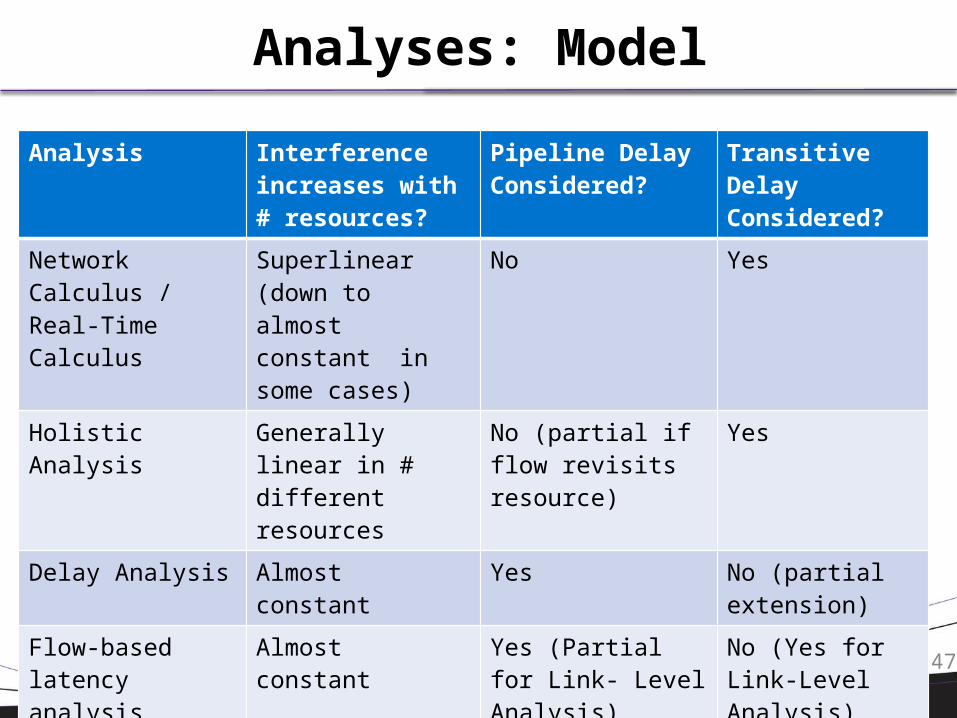
Analyses: Model

Analysis Interference increases with # resources?

Pipeline Delay Considered?

Transitive Delay Considered?

Network Calculus / Real-Time Calculus

Superlinear (down to almost constant in some cases)

No Yes

Holistic Analysis Generally linear in # different resources

No (partial if flow revisits resource)

Yes

Delay Analysis Almost constant Yes No (partial extension)

Flow-based latency analysis

Almost constant Yes (Partial for Link- Level Analysis)

No (Yes for Link-Level Analysis)

7

Holistic Analysis

8 / 47

Transaction Model (Tasks with Offsets)• Fast and Tight Response-Times for Tasks with Offsets• Schedulability Analysis for Tasks with Static and Dynamic

Offsets. • Improved Schedulability Analysis of Real-Time

Transactions with Earliest Deadline Scheduling

9 / 47

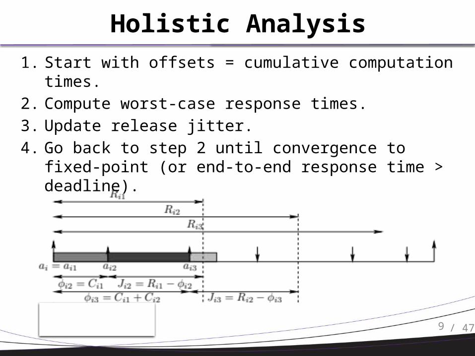
Holistic Analysis

1. Start with offsets = cumulative computation times.

2. Compute worst-case response times.

3. Update release jitter.

4. Go back to step 2 until convergence to fixed-point (or end-to-end response time > deadline).

10 / 47

Can you model Wormhole Routing?• Sure you can!

• For a flow with K flits, simply assume there are K transactions– Assign artificially decreasing priorities to the K transactions

to best model the precedence constraint among flits.

• The problem is that response time analysis for transaction models do not take into account relations among different resources – can not take advantage of pipeline delay.

11 / 47

Response Time Analysis• Let’s focus on a single resource – note a flow might visit a

resource multiple times.• The worst-case is produced when a task for each interfering

transaction is released at the critical instant after suffering worst-case jitter.– Tasks activated before the critical instant are delayed (by jitter)

until the critical instant if feasible– Tasks activated after the critical instant suffer no jitter

• EDF: the task under analysis has deadline = to the deadline of any interfering task in the busy period

• RM: a task of the transaction under analysis is released at the critical instant– Same assumptions for all other tasks of the transactions– In both cases, we need to try out all possibilities

12 / 47

Response Time Analysis• Problem: the number of possible activation patterns is

exponential– For each interfering transaction, we can pick any task– Hence the number of combinations is exponential in the

number of transactions.• Solution: compute a worst-case interference pattern over all

possible starting tasks for a given interfering transaction.• For the transaction under analysis we still analyze all

possible patterns.

13 / 47

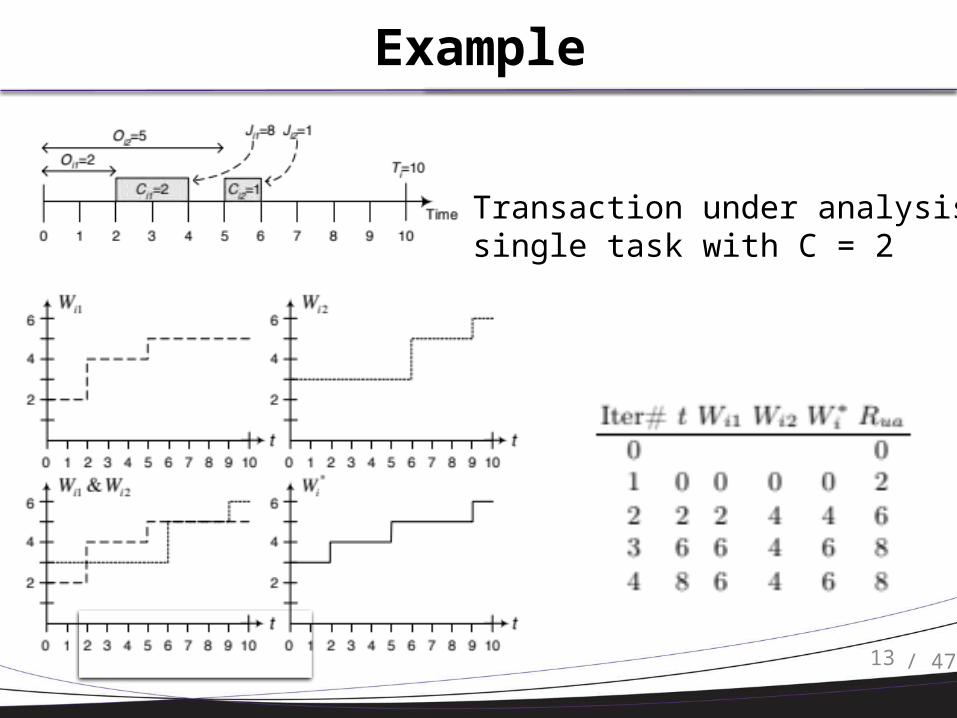
Example

Transaction under analysis: single task with C = 2

14 / 47

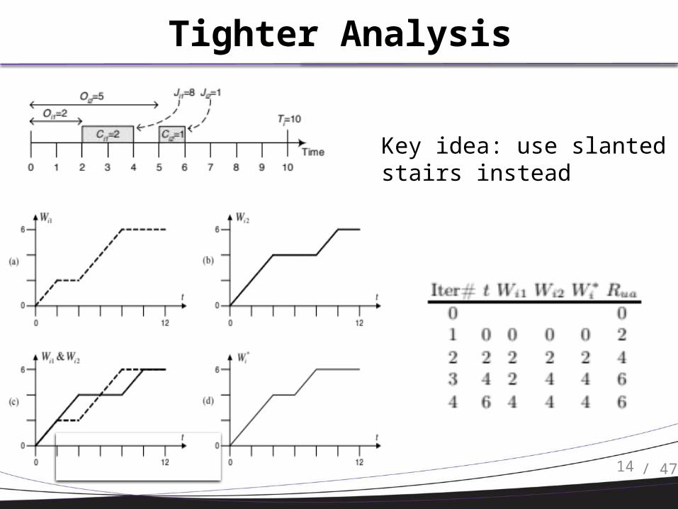
Tighter Analysis

Key idea: use slanted stairs instead

15 / 47

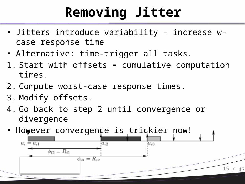
Removing Jitter• Jitters introduce variability – increase w-case response time• Alternative: time-trigger all tasks.

1. Start with offsets = cumulative computation times.

2. Compute worst-case response times.

3. Modify offsets.

4. Go back to step 2 until convergence or divergence• However convergence is trickier now!

16 / 47

Cyclic-Dynamic Offsets• Response time can decrease as a result of modifying offsets.

– Always increasing as jitter increases• We can prove that it is sufficient to check for limit cycles.

17 / 47

Pipeline Delay

• T2 higher priority. All Ctime = 1. With Jitter…

O = 0 R = 2 J = 0

O = 2 R = 7!J = 2

O = 1 R = 4J = 1

O = 4 R = 11J = 5

O = 5 R = 13J = 6

O = 6 R = 15J = 7

O = 3 R = 9J = 4

18 / 47

Pipeline Delay

• T2 higher priority. All Ctime = 1. With Offsets…

O = 0 R = 2

O = 4 R = 6

O = 2 R = 4

O = 8 R = 10

O = 10 R = 12

O = 12 R = 14

O = 6 R = 8

19

Delay Calculus

20 / 47

Delay Calculus• End-To-End Delay Analysis of Distributed Systems with Cycles

in the Task Graph• System Model:

– Aperiodic flows (each called a job)– Each job has the same fixed priority on all resources (nodes)– Arbitrary path through nodes (stages) – can include cycles– Each stage can have a different computation time

• How to model worm-hole routing– Use one job for each flit

21 / 47

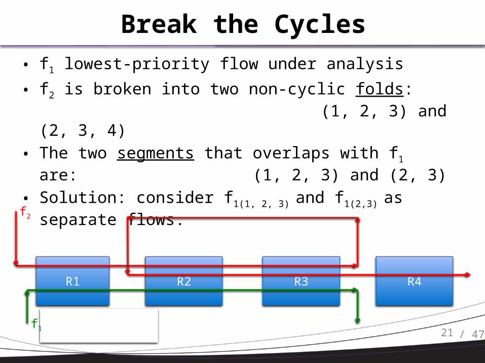
Break the Cycles

• f1 lowest-priority flow under analysis

• f2 is broken into two non-cyclic folds: (1, 2, 3) and (2, 3, 4)

• The two segments that overlaps with f1 are: (1, 2, 3) and (2, 3)

• Solution: consider f1(1, 2, 3) and f1(2,3) as separate flows.

R1 R2 R3 R4

f2

f1

22 / 47

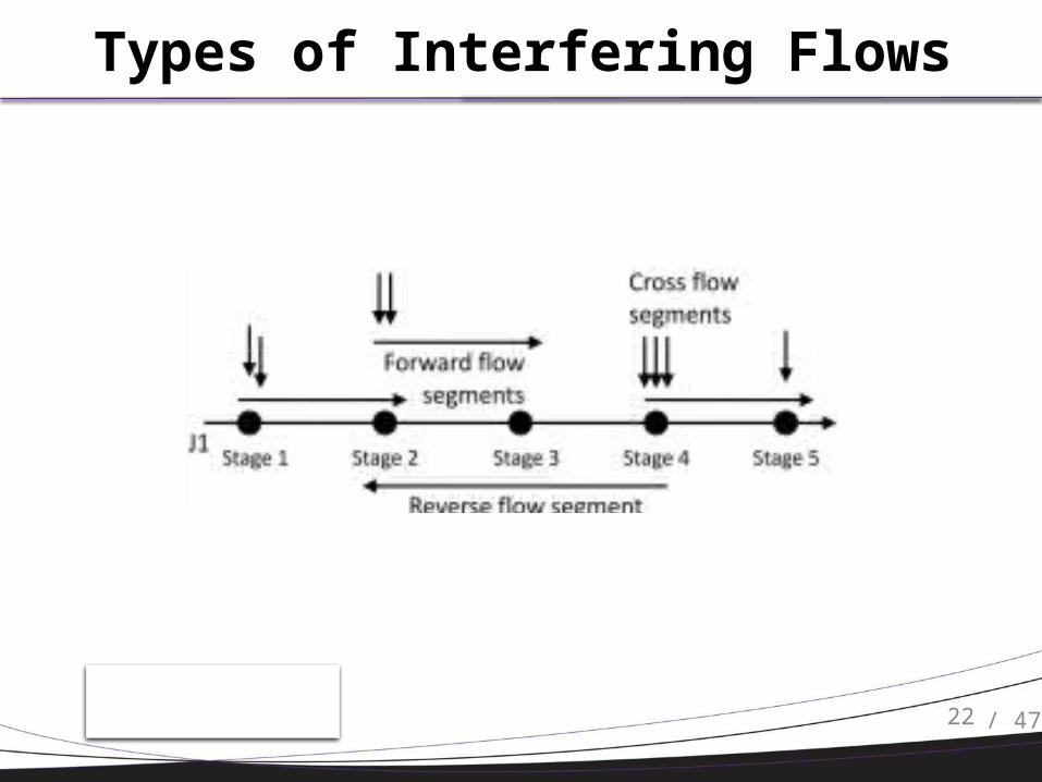
Types of Interfering Flows

23 / 47

Execution Trace• Earliest trace: earliest job finishing time on each stage such

that there is no idle time at the end.

24 / 47

Delay Bounds• Each cross-flow segment and reserve-flow segment

contributes one stage computation time to the earliest trace• What about forward flows?

S1 f1 f2

S2 f1f2

S3 f2

S4 f2

f1

f1

f2 on the last stage it delays f1

f2 preempting lower-priority job one execution of the longestjob on each stage

25 / 47

Delay Bounds

• Preemptive Case:

• Non-Preemptive Case:

2 max executions for each higher priority segment Max exec time

for each stage

No preemption meansone max execution forhigher priority segment…

… but we have to pay onemax execution of blocking time on each stage

26 / 47

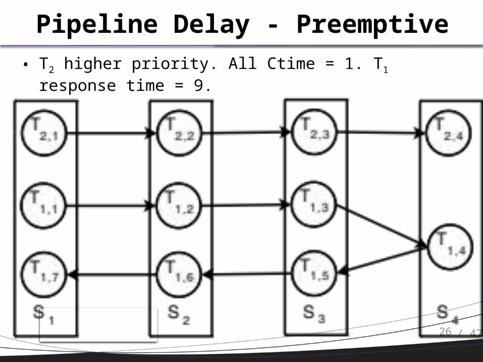
Pipeline Delay - Preemptive

• T2 higher priority. All Ctime = 1. T1 response time = 9.

27 / 47

The Periodic Case • Now assume jobs are produced by periodic activations…• Trick: reduce cyclic system to an equivalent uniprocessor

system. For preemptive case:– Replace each segment with a periodic task with ctime =

– Replace the flow under analysis with a task with ctime =

• Schedulability can then be checked with any uniprocessor test (utilization bound, response time analysis).

28 / 47

Transitive Delay

• All Ctime = 1, non-preemptive.

• Let’s assume T2 = T3 = 2, deadline = period.

• Then U2 = ½, U3 = ½ and the system is not schedulable…

• In reality the worst-case response time of f1 is 4.

S1 S2

f1

f2f3

29 / 47

Other issues…• What happens if deadline > period?

– Add an addition floor(deadline/period) instances of the higher priority job.

– Self blocking: the flow under analysis can block itself. Hence, consider its previous instances as another, higher priority flow.

• What happens if a flow suffers jitter (i.e., indirect blocking)?– Add an additional ceil(jitter/period) instances.– Note: all reverse flows have this issue…

• Lots of added terms -> bad analysis for low number of stages.

30 / 47

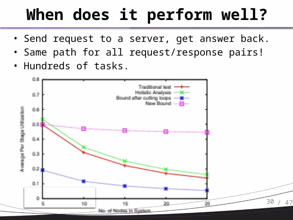
When does it perform well?• Send request to a server, get answer back.• Same path for all request/response pairs!• Hundreds of tasks.

31

Network Calculus

32 / 47

Aggregate Traffic• Assumption: we do not know the arbitration employed by

the router.• Solution: consider each flow as the lowest-priority one.

33 / 47

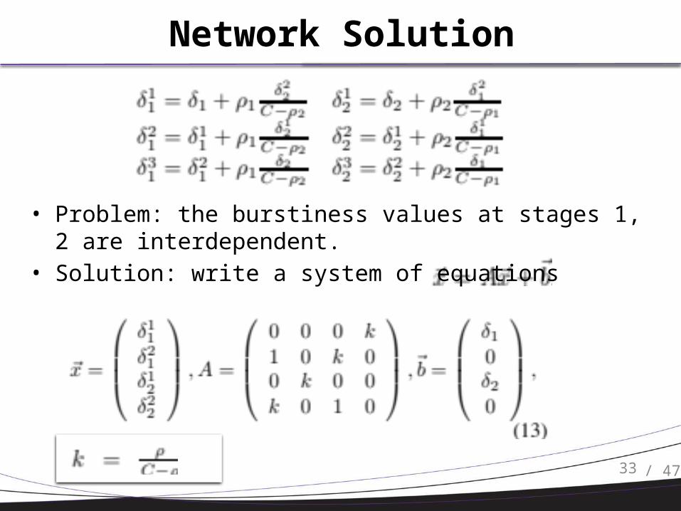
Network Solution

• Problem: the burstiness values at stages 1, 2 are interdependent.

• Solution: write a system of equations

34 / 47

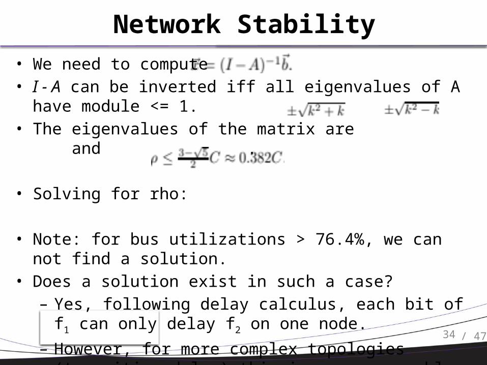
Network Stability• We need to compute • I - A can be inverted iff all eigenvalues of A have module <= 1.• The eigenvalues of the matrix are and .

• Solving for rho:

• Note: for bus utilizations > 76.4%, we can not find a solution.• Does a solution exist in such a case?

– Yes, following delay calculus, each bit of f1 can only delay f2 on one node.

– However, for more complex topologies (transitive delay) this is an open problem.

35

Modular performance analysis

36 / 47

Modular Performance Analysis• System Architecture evaluation using modular performance

analysis: a case study

• An application of network calculus to early system performance analysis and design exploration.

• Real-time calculus: extension to network-calculus.– Introduces lower arrival curves and upper service curves– A more structured approach to system description and

multiple flows analysis

37 / 47

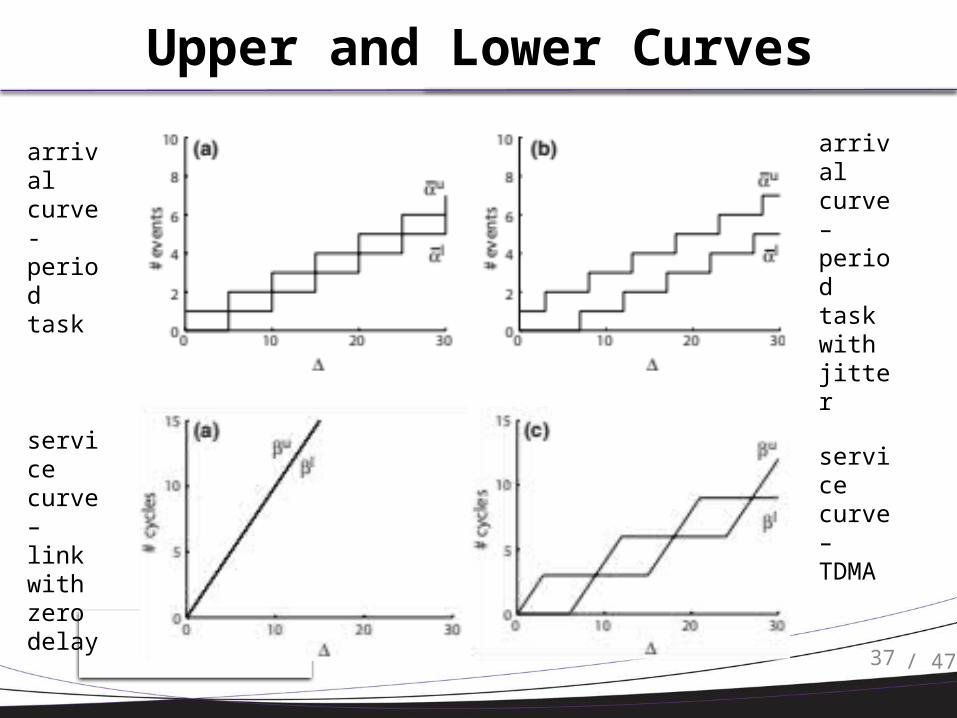
Upper and Lower Curves

arrival curve - periodtask

arrival curve – periodtaskwith jitter

service curve – link with zero delay

service curve – TDMA

38 / 47

Abstract Component

39 / 47

Network of Components

40 / 47

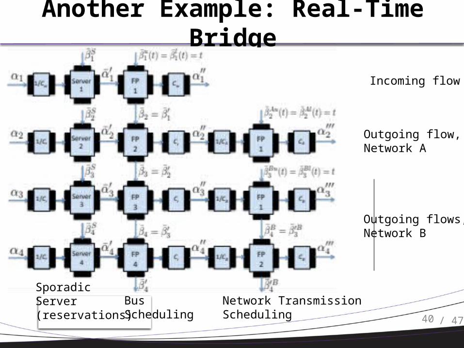
Another Example: Real-Time Bridge

Incoming flow

Outgoing flow, Network A

Outgoing flows, Network B

SporadicServer(reservations)

Bus Scheduling

Network TransmissionScheduling

41 / 47

Design Flow

42 / 47

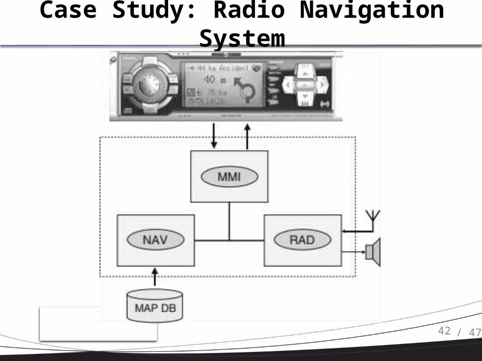
Case Study: Radio Navigation System

43 / 47

Example: Change Volume Sequence Diagram

44 / 47

Architectural Alternatives

45 / 47

Model: Architecture A

46 / 47

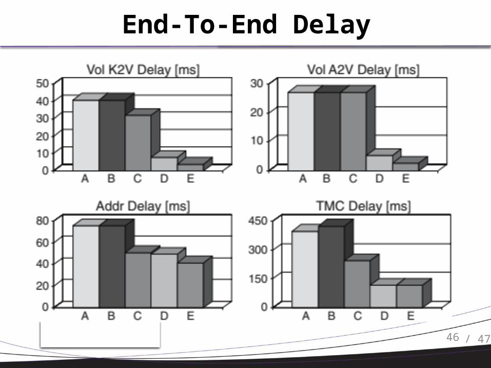
End-To-End Delay

47 / 47

Sensitivity to Resource Capacity