ece257 numerical methods and scientific computingchandy/courses/257f04/257ln01.pdf ·...
TRANSCRIPT

ECE257ECE257 NumericalNumerical Methods Methods andandScientificScientific ComputingComputing
John A. ChandyJohn A. Chandy

ECE 257 Numerical Methods and Scientific Computing
Fall 2004
Lecture 1
John A. Chandy
Dept. of Electrical and Computer Engineering
University of Connecticut
TodayToday’’s class:s class:
•• Introduction to numerical methodsIntroduction to numerical methods
•• Basic content of course and classBasic content of course and classexpectationsexpectations
•• Mathematical modelingMathematical modeling

ECE 257 Numerical Methods and Scientific Computing
Fall 2004
Lecture 1
John A. Chandy
Dept. of Electrical and Computer Engineering
University of Connecticut
IntroductionIntroduction•• What are numerical methods?What are numerical methods?
–– ““…… techniques by which mathematical problems are techniques by which mathematical problems areformulated so that they can be solved with arithmeticformulated so that they can be solved with arithmeticoperations.operations.”” (Chopra and Canale) (Chopra and Canale)
•• What type of mathematical problems?What type of mathematical problems?
–– RootsRoots
–– IntegrationIntegration
–– OptimizationOptimization
–– Curve FittingCurve Fitting
–– Differential EquationsDifferential Equations
–– Linear SystemsLinear Systems

ECE 257 Numerical Methods and Scientific Computing
Fall 2004
Lecture 1
John A. Chandy
Dept. of Electrical and Computer Engineering
University of Connecticut
IntroductionIntroduction
•• How do you solve these difficult mathematicalHow do you solve these difficult mathematicalproblems?problems?
•• Example: What are the roots of xExample: What are the roots of x22-7x+12?-7x+12?
•• Three general non-computer methodsThree general non-computer methods
–– AnalyticalAnalytical
–– GraphicalGraphical
–– ManualManual
ECE 257 Numerical Methods and Scientific Computing
Fall 2004
Lecture 1
John A. Chandy
Dept. of Electrical and Computer Engineering
University of Connecticut
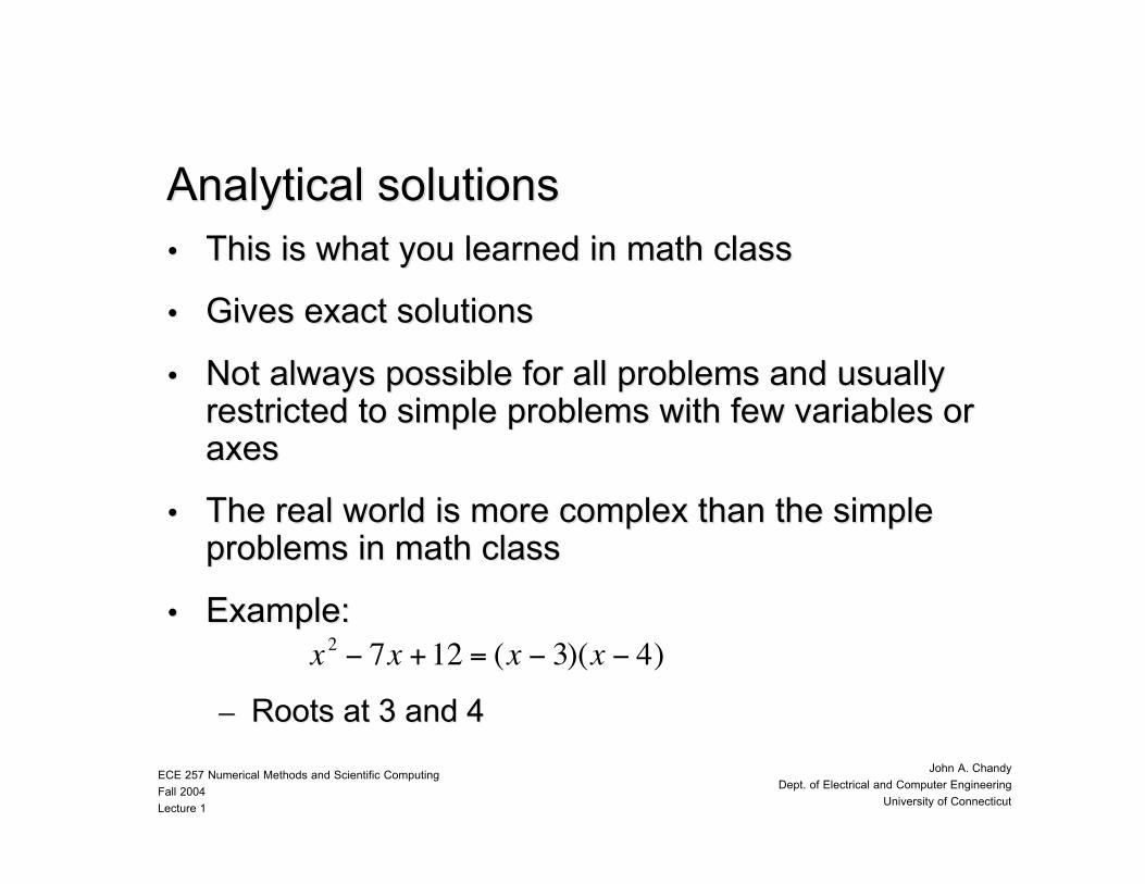
Analytical solutionsAnalytical solutions•• This is what you learned in math classThis is what you learned in math class
•• Gives exact solutionsGives exact solutions
•• Not always possible for all problems and usuallyNot always possible for all problems and usuallyrestricted to simple problems with few variables orrestricted to simple problems with few variables oraxesaxes
•• The real world is more complex than the simpleThe real world is more complex than the simpleproblems in math classproblems in math class
•• Example:Example:
–– Roots at 3 and 4Roots at 3 and 4
€
x 2 − 7x +12 = (x − 3)(x − 4)

ECE 257 Numerical Methods and Scientific Computing
Fall 2004
Lecture 1
John A. Chandy
Dept. of Electrical and Computer Engineering
University of Connecticut
Graphical SolutionGraphical Solution
-10
0
10
20
30
40
50
60
70
80
-6 -4 -2 0 2 4 6

ECE 257 Numerical Methods and Scientific Computing
Fall 2004
Lecture 1
John A. Chandy
Dept. of Electrical and Computer Engineering
University of Connecticut
Manual SolutionManual Solution
•• Using pen and paper, calculators, slideUsing pen and paper, calculators, sliderules, etc. to solve an engineering problemrules, etc. to solve an engineering problem
•• Very time consumingVery time consuming
•• Error-proneError-prone

ECE 257 Numerical Methods and Scientific Computing
Fall 2004
Lecture 1
John A. Chandy
Dept. of Electrical and Computer Engineering
University of Connecticut
IntroductionIntroduction
•• What are numerical methods?What are numerical methods?
–– ““…… techniques by which mathematical problems are techniques by which mathematical problems areformulated so that they can be solved with arithmeticformulated so that they can be solved with arithmeticoperations.operations.”” (Chopra and Canale) (Chopra and Canale)
•• Arithmetic operations map into computer arithmeticArithmetic operations map into computer arithmeticinstructionsinstructions
•• Numerical methods allow us to formulateNumerical methods allow us to formulatemathematical problems so they can be solved bymathematical problems so they can be solved bycomputercomputer
ECE 257 Numerical Methods and Scientific Computing
Fall 2004
Lecture 1
John A. Chandy
Dept. of Electrical and Computer Engineering
University of Connecticut
Course OverviewCourse Overview
•• What is this course about?What is this course about?
–– Using computers and numerical methods toUsing computers and numerical methods tosolve mathematical problems that arise insolve mathematical problems that arise inengineeringengineering
–– Most of the focus will be on electricalMost of the focus will be on electricalengineering problemsengineering problems

ECE 257 Numerical Methods and Scientific Computing
Fall 2004
Lecture 1
John A. Chandy
Dept. of Electrical and Computer Engineering
University of Connecticut
Class meetings:Class meetings:
•• Lectures are Lectures are Tuesday and Thursday,Tuesday and Thursday,1111––12:1512:15
•• No specific lab time, but significantNo specific lab time, but significantcomputer time expected.computer time expected.
•• Computers are available in C25 and C27.Computers are available in C25 and C27.

ECE 257 Numerical Methods and Scientific Computing
Fall 2004
Lecture 1
John A. Chandy
Dept. of Electrical and Computer Engineering
University of Connecticut
Class Class assignmentsassignments
•• Homework will be Homework will be assignedassigned once every once every week or twoweek or twoand due usually the following week.and due usually the following week.
•• You may collaborate on the homework, but yourYou may collaborate on the homework, but yoursubmissions should be your own work.submissions should be your own work.
•• Grading:Grading:
–– HomeworksHomeworks 40%40%
–– Exam 1 and 2Exam 1 and 2 40%40%
–– Final ExamFinal Exam 20%20%
ECE 257 Numerical Methods and Scientific Computing
Fall 2004
Lecture 1
John A. Chandy
Dept. of Electrical and Computer Engineering
University of Connecticut
Mathematical BackgroundMathematical Background
•• MATH 210Q/211QMATH 210Q/211Q
•• Taylor seriesTaylor series
•• Differentiation/IntegrationDifferentiation/Integration
•• Linear AlgebraLinear Algebra
ECE 257 Numerical Methods and Scientific Computing
Fall 2004
Lecture 1
John A. Chandy
Dept. of Electrical and Computer Engineering
University of Connecticut
Computer BackgroundComputer Background
•• Languages toLanguages to be covered: be covered:
–– C, C++, Fortran, C, C++, Fortran, MatlabMatlab
•• CSE 123/124 programming experienceCSE 123/124 programming experience
•• Any OS is acceptableAny OS is acceptable
ECE 257 Numerical Methods and Scientific Computing
Fall 2004
Lecture 1
John A. Chandy
Dept. of Electrical and Computer Engineering
University of Connecticut
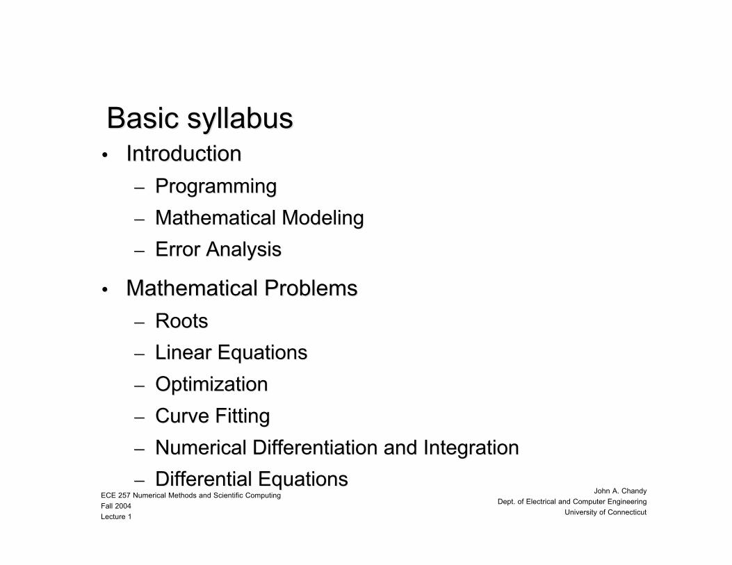
Basic syllabusBasic syllabus•• IntroductionIntroduction
–– ProgrammingProgramming
–– Mathematical ModelingMathematical Modeling
–– Error AnalysisError Analysis
•• Mathematical ProblemsMathematical Problems
–– RootsRoots
–– Linear EquationsLinear Equations
–– OptimizationOptimization
–– Curve FittingCurve Fitting
–– Numerical Differentiation and IntegrationNumerical Differentiation and Integration
–– Differential EquationsDifferential Equations

ECE 257 Numerical Methods and Scientific Computing
Fall 2004
Lecture 1
John A. Chandy
Dept. of Electrical and Computer Engineering
University of Connecticut
Mathematical ModelingMathematical Modeling
A A mathematical modelmathematical modelis the formulation of ais the formulation of aphysical or engineeringphysical or engineeringsystem in mathematicalsystem in mathematicalterms.terms.
EmpiricalEmpirical
TheoreticalTheoretical

ECE 257 Numerical Methods and Scientific Computing
Fall 2004
Lecture 1
John A. Chandy
Dept. of Electrical and Computer Engineering
University of Connecticut
Mathematical ModelingMathematical Modeling
•• Dependent variable = Dependent variable = f f (( independent variables, independent variables, parameters, parameters, forcing functions )forcing functions )
•• In an electrical circuit, I = V/R; The current, I, isIn an electrical circuit, I = V/R; The current, I, isdependent on resistance parameter, R, and forcingdependent on resistance parameter, R, and forcingvoltage function, V.voltage function, V.

ECE 257 Numerical Methods and Scientific Computing
Fall 2004
Lecture 1
John A. Chandy
Dept. of Electrical and Computer Engineering
University of Connecticut
Example 1Example 1
•• What is the velocity of a falling object?What is the velocity of a falling object?
–– First step is to model the systemFirst step is to model the system
–– NewtonNewton’’s second laws second law
–– Total force is gravity and air resistanceTotal force is gravity and air resistance
€
F = ma⇒ a =Fm⇒
dvdt
=Fm
€
F = FGravity + FAir = mg− cv

ECE 257 Numerical Methods and Scientific Computing
Fall 2004
Lecture 1
John A. Chandy
Dept. of Electrical and Computer Engineering
University of Connecticut
Example 1Example 1
–– First order differential equationFirst order differential equation
–– Analytical solutionAnalytical solution€
dvdt
=Fm
=mg− cvm
= g − cmv
€
v(t) =gmc1− e
−cmt

ECE 257 Numerical Methods and Scientific Computing
Fall 2004
Lecture 1
John A. Chandy
Dept. of Electrical and Computer Engineering
University of Connecticut
Example 1Example 1
•• m=68.1kg, c=12.5 kg/sm=68.1kg, c=12.5 kg/s

ECE 257 Numerical Methods and Scientific Computing
Fall 2004
Lecture 1
John A. Chandy
Dept. of Electrical and Computer Engineering
University of Connecticut
Example 1Example 1
•• What if we canWhat if we can’’t find an analytical solution?t find an analytical solution?
•• How do you get a computer to solve theHow do you get a computer to solve thedifferential equation?differential equation?
•• Use numerical methodsUse numerical methods

ECE 257 Numerical Methods and Scientific Computing
Fall 2004
Lecture 1
John A. Chandy
Dept. of Electrical and Computer Engineering
University of Connecticut
EulerEuler’’s Methods Method
•• Use the Use the finite divided differencefinite divided difference approximation approximationof the derivativeof the derivative
•• The approximation becomes exact as The approximation becomes exact as ∆∆t t →→ 00
€
dvdt
≅v ti+1( ) − v ti( )ti+1 − ti
ECE 257 Numerical Methods and Scientific Computing
Fall 2004
Lecture 1
John A. Chandy
Dept. of Electrical and Computer Engineering
University of Connecticut
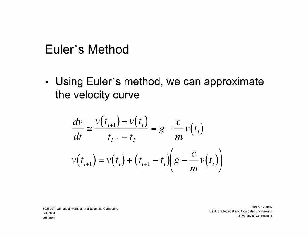
EulerEuler’’s Methods Method
•• Using EulerUsing Euler’’s method, we can approximates method, we can approximatethe velocity curvethe velocity curve
€
dvdt
≅v ti+1( ) − v ti( )ti+1 − ti
= g − cmv ti( )
v ti+1( ) = v ti( ) + ti+1 − ti( ) g − cmv ti( )

ECE 257 Numerical Methods and Scientific Computing
Fall 2004
Lecture 1
John A. Chandy
Dept. of Electrical and Computer Engineering
University of Connecticut
EulerEuler’’s Methods Method
•• Assume Assume ∆∆t=2t=2
€
v 0( ) = 0
v 2( ) = v 0( ) + 2 g − cmv 0( )
=19.6
v 4( ) = v 2( ) + 2 g − cmv 2( )
= 32.0
M

ECE 257 Numerical Methods and Scientific Computing
Fall 2004
Lecture 1
John A. Chandy
Dept. of Electrical and Computer Engineering
University of Connecticut
EulerEuler’’s methods method
ECE 257 Numerical Methods and Scientific Computing
Fall 2004
Lecture 1
John A. Chandy
Dept. of Electrical and Computer Engineering
University of Connecticut
EulerEuler’’s methods method
•• Avoids solving differential equationAvoids solving differential equation
•• Not an exact approximation of the functionNot an exact approximation of the function
•• Gets more exact as Gets more exact as ∆∆tt→→00
•• How do we choose How do we choose ∆∆t? Dependent on ourt? Dependent on ourtolerance of error.tolerance of error.
•• How do we estimate the error?How do we estimate the error?

ECE 257 Numerical Methods and Scientific Computing
Fall 2004
Lecture 1
John A. Chandy
Dept. of Electrical and Computer Engineering
University of Connecticut
Mathematical ModelingMathematical Modeling
•• Conservation LawsConservation Laws
–– Change = increases - decreasesChange = increases - decreases
•• In steady state, change = 0In steady state, change = 0
•• Increases = decreasesIncreases = decreases
–– Examples:Examples:
•• KirchoffKirchoff’’s Current and Voltage Lawss Current and Voltage Laws
•• Fluid flow (flow in = flow out)Fluid flow (flow in = flow out)

ECE 257 Numerical Methods and Scientific Computing
Fall 2004
Lecture 1
John A. Chandy
Dept. of Electrical and Computer Engineering
University of Connecticut
Example 2Example 2
+-
i(t)C
t=0
V
Find vC(t)
R

ECE 257 Numerical Methods and Scientific Computing
Fall 2004
Lecture 1
John A. Chandy
Dept. of Electrical and Computer Engineering
University of Connecticut
Example 2Example 2
•• Analytical solutionAnalytical solution
€
V = Ri(t) + vC (t)
i(t) = C dvCdt
dvCdt
=1RC
V − vC (t)( )
€
vC (t) =V 1− e−
tRC
i(t) = C dvCdt
=VRe−
tRC

ECE 257 Numerical Methods and Scientific Computing
Fall 2004
Lecture 1
John A. Chandy
Dept. of Electrical and Computer Engineering
University of Connecticut
Example 2Example 2
•• Numerical solutionNumerical solution
€
V = Ri(t) + vC (t)
0 = R didt
+dvCdt
0 = R didt
+i(t)C
didt
= −1RC
i(t)

ECE 257 Numerical Methods and Scientific Computing
Fall 2004
Lecture 1
John A. Chandy
Dept. of Electrical and Computer Engineering
University of Connecticut
Example 2Example 2
•• Intial value of i(t)=V/RIntial value of i(t)=V/R
€
didt
= −1RC
i(t j ) =i t j+1( ) − i t j( )t j+1 − t j
i t j+1( ) = i t j( ) − t j+1 − t j( )i t j( )RC
i(0) =V R
i(2) = i(0) − 2 i 0( )RC
=VR1− 2
RC
M

ECE 257 Numerical Methods and Scientific Computing
Fall 2004
Lecture 1
John A. Chandy
Dept. of Electrical and Computer Engineering
University of Connecticut
Next classNext class
•• Programming and SoftwareProgramming and Software
•• Read Chapters 1 & 2Read Chapters 1 & 2