ECE295,  Data  Assimila0on  and  Inverse  Problems,  Spring  2015  Peter  Gersto),  534-­‐7768,  gersto)@ucsd.edu  We  meet  Wednesday  from  5  to  6:20pm  in  HHS  2305A  Text  for  first  5  classes:  Parameter  EsGmaGon  and  Inverse  Problems  (2nd  EdiGon)    here  under  UCSD  license  Grading    S  Classes  1  April,  Intro;  Linear  discrete  Inverse  problems    (Aster  Ch  1,  2)      8  April,    SVD  (Aster  ch  2  and  3)    15  April,  RegularizaGon  (ch  4)                                                                                                            Numerical  Example:  Beamforming  22  April,  Sparse  methods  (ch  7.2-­‐7.3)    29  April,  Sparse  methods  6  May,    Bayesian  methods  and  Monte  Carlo  methods  (ch  11)                                          Numerical  Example:  Ice–flow  from  GPS  13  May,  IntroducGon  to  sequenGal  Bayesian  methods,  Kalman  Filter    20  May,    Data  assimilaGon,  EnKF    27  May,      EnKF,    Data  assimilaGon    3  June,      Markov  Chain  Monte  Carlo,  PF      Homework:  Call  the  files  LastName_ExXX.    Homework  is  due  8am  on  Wednesday.  That  way  we  can  discuss  in  class.  Hw  1:  Download  the  matlab  codes  for  the  book  (cd_5.3).  Run  the  3  examples  for  chapter  2.  Come  to  class  with  one  quesGon  about  the  examples  Hw2:  Based  on  Example  3.3.  Adapt  it  to  a  complex  valued  beamforming  example.  %  Parameters  c  =  1500;              %  speed  of  sound  f  =  200;                %  frequency  lambda  =  c/f;      %  wavelength  k  =  2*pi/lambda;%  wavenumber      %  ULA-­‐horizontal  N  =  20;                  %  number  of  sensors  d  =  1/2*lambda;  %  intersensor  spacing  q  =  [0:1:(N-­‐1)];%  sensor  numbering  xq  =  (q-­‐(N-­‐1)/2)*d;  %  sensor  locaGons      

Beamforming  example  %  Parameters  c  =  1500;              %  speed  of  sound  f  =  200;                %  frequency  lambda  =  c/f;      %  wavelength  k  =  2*pi/lambda;%  wavenumber      %  ULA-­‐horizontal  N  =  20;                  %  number  of  sensors  d  =  1/2*lambda;  %  intersensor  spacing  q  =  [0:1:(N-­‐1)];%  sensor  numbering  xq  =  (q-­‐(N-­‐1)/2)*d;  %  sensor  locaGons  %  Bearing  grid  theta  =  [-­‐90:0.5:90];  u  =  sind(theta);      %  RepresenaGon  matrix  (steering  matrix)  A  =  exp(-­‐1i*2*pi/lambda*xq'*u)/sqrt(N);          

•  REVIEW  

4  

EsGmaGon  and  Appraisal  

 

5

Over-determined: Linear discrete inverse problem

We seek the model vector m which minimizes

Note that this is a quadratic function of the model vector.Solution: Differentiate with respect to m and solve for the model vector which gives a zero gradient in

This is the least-squares solution.

A solution to the normal equations:

This gives…

3

Compare with maximum likelihood

6

Over-determined: Linear discrete inverse problem

How does the Least-squares solution compare to the standard equations of linear regression ?

Given N data yi with independent normally distributed errors and standard deviations Vi what are the expressions for the model parameters m = [a,b]T ?

7

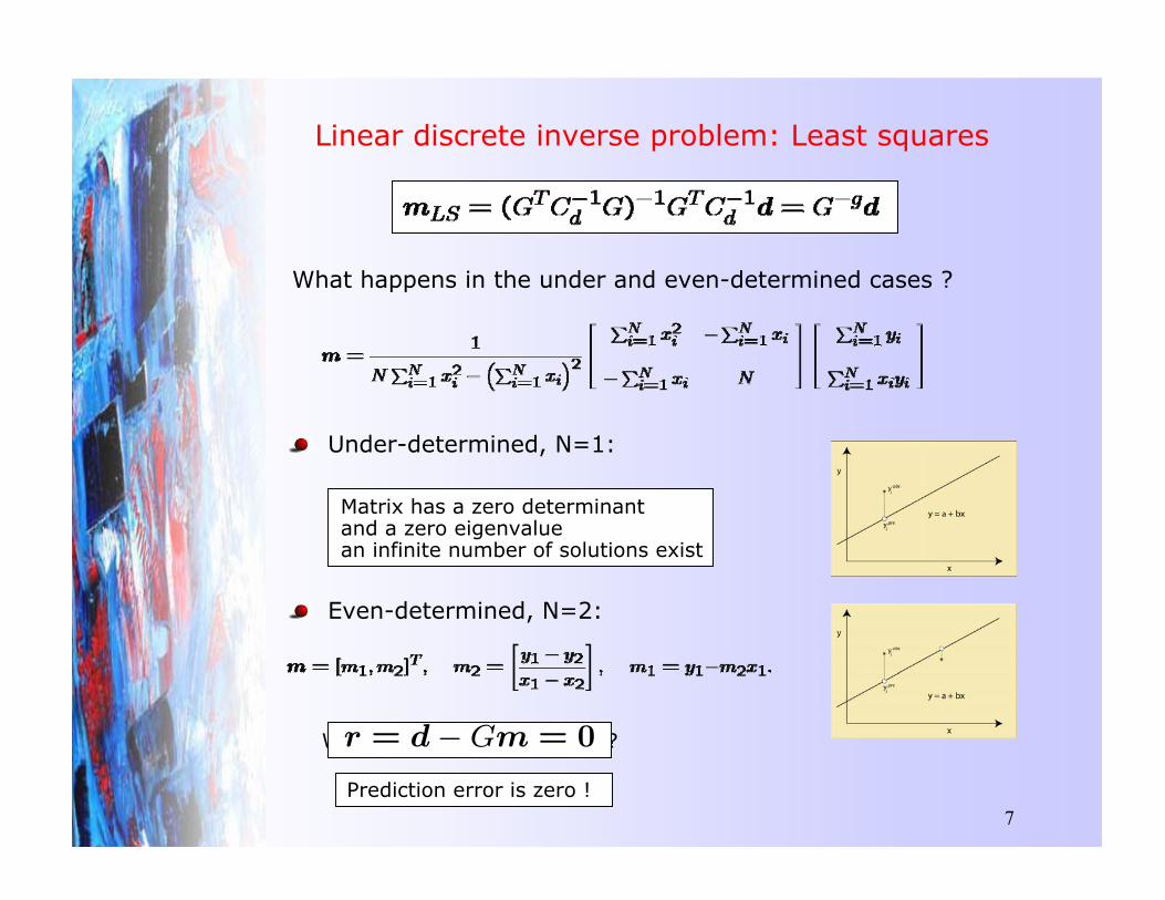
What is m ?

What is the prediction error ?

Linear discrete inverse problem: Least squares

What happens in the under and even-determined cases ?

Matrix has a zero determinant and a zero eigenvaluean infinite number of solutions exist

Under-determined, N=1:

Even-determined, N=2:

Prediction error is zero !

r = dcGm= 0

8

Example: Over-determined, Linear discrete inverse problem

Given data and noise

The Ballistics example

Calculate G

Is the data fit good enough ?

And how to errors in data propagateinto the solution ?

9

The two questions in parameter estimation

We need to:Assess the quality of the data fit.

Estimate how errors in the data propagate into the model

We have our fitted model parameters

…but we are far from finished !

Goodness of fit: Does the model fit the data to within the statistical uncertainty of the noise ?

What are the errors on the model parameters ?

10

Goodness of fit

Once we have our least squares solution mLS how do we know whether the fit is good enough given the errors in the data ?

Use the prediction error at the least squares solution !

If data errors are Gaussian this as a chi-square statistic

16

Goodness of fit

For Gaussian data errors the data prediction error is the square of a Gaussian random variable hence it has a chi-square probability density function with N-M degrees of freedom.

ndf �2(5%) �2(50%) �2(95%)5 1.15 4.35 11.0710 3.94 9.34 18.3120 10.85 19.34 31.4150 34.76 49.33 67.50100 77.93 99.33 124.34

The test provides a means to testing the assumptions that went into producing the least squares solution. It gives the likelihood that the fit actually achieved is reasonable.

p = 0.05p = 0.95

17

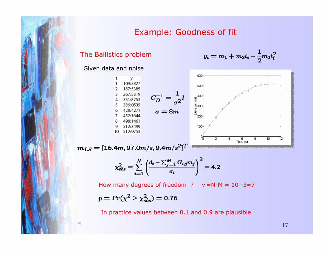
Example: Goodness of fit

Given data and noise

The Ballistics problem

How many degrees of freedom ? Q =N-M = 10 -3=7

In practice values between 0.1 and 0.9 are plausible

4

19

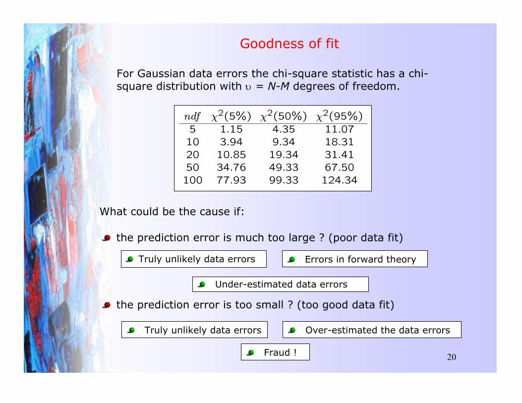
Goodness of fit

For Gaussian data errors the chi-square statistic has a chi-square distribution with X = N-M degrees of freedom.

ndf �2(5%) �2(50%) �2(95%)5 1.15 4.35 11.0710 3.94 9.34 18.3120 10.85 19.34 31.4150 34.76 49.33 67.50100 77.93 99.33 124.34

If I fit 7 data points with a straight line and getwhat would you conclude ?

If I fit 102 data points with a straight line and getwhat would you conclude ?

If I fit 52 data points with a straight line and getwhat would you conclude ?

Exercise:

20

Goodness of fit

For Gaussian data errors the chi-square statistic has a chi-square distribution with X = N-M degrees of freedom.

ndf �2(5%) �2(50%) �2(95%)5 1.15 4.35 11.0710 3.94 9.34 18.3120 10.85 19.34 31.4150 34.76 49.33 67.50100 77.93 99.33 124.34

the prediction error is too small ? (too good data fit)

the prediction error is much too large ? (poor data fit)

Truly unlikely data errors Errors in forward theory

What could be the cause if:

Truly unlikely data errors Over-estimated the data errors

Fraud !

Under-estimated data errors

SoluGon  Appraisal  

21

Solution error Once we have our least squares solution mLS and we know that the data fit is acceptable, how do we find the likely errors in the model parameters arising from errors in the data ?

d0 � d+ ²

The data set we actually observed is only one realization of the many that could have been observed

mLS + ²m = Gcg(d+ ²)

²m = Gcg²

The effect of adding noise to the data is to add noise to the solution

mLS = Gcgd

The model noise is a linear combination of the data noise !

m0LS �mLS + ²m

m0LS = Gcgd0

22

Solution error: Model Covariance

Multivariate Gaussian data error distribution

How to turn this into a probability distribution for the model errors ?

We know that the solution error is a linear combination of the data error

The covariance of any linear combination Ad of Gaussian distributed random variables d is

So we have the covariance of the model parameters

²m = Gcg²

23

Solution error: Model Covariance

The data error distribution gives a model error distribution !

is the least squares solution

The model covariance for a least squares problem depends on data errors and not the data itself ! G is controlled by the design of the experiment.

24

Solution error: Model Covariance

For the special case of independent data errors

For linear regression problem

Independent data errors Correlated model errors

26

Example: Model Covariance and confidence intervals

For Ballistics problem

95% confidence interval for parameter i

27

Confidence intervals by projection The M-dimensional confidence ellipsoid can be projected onto any subset (or

combination) of ' parameters to obtain the corresponding confidence ellipsoid.

Full M-dimensional ellipsoid

Projected Q dimension ellipsoid

Projected model vectorProjected covariance matrix

Chosen percentage point of the F2

Q distribution

To find the 90% confidence ellipse for (x,y) from a 3-D (x,y,z) ellipsoid

Can you see that this procedure gives the same formula for the 1-D case obtained previously ?

32

What if we do not know the errors on the data ?

Both Chi-square goodness of fit tests and model covariance Calculations require knowledge of the variance of the data.

What can we do if we do not know V ?

Consider the case of

CD = ~2IIndependent data errors

Calculated from least squares solution

So we can still estimate model errors using the calculated data errorsbut we can no long claim anything about goodness of fit.

34

Model Resolution matrix

If we obtain a solution to an inverse problem we can ask what its relationship is to the true solution

mest = Gcgd

d = Gmtrue

But we knowBut we know

and henceand hence

mest = GcgGmtrue = Rmtrue

The matrix R measures how `good an inverse’ GThe matrix R measures how `good an inverse’ G--gg is.is.

The matrix R shows how the elements of The matrix R shows how the elements of mmestest are built from are built from linear combination of the true model, linear combination of the true model, mmtruetrue. Hence matrix R . Hence matrix R measures the amount of measures the amount of blurringblurring produced by the inverse produced by the inverse operator.operator.

For the least squares solution we haveFor the least squares solution we have

� R = IGcg = (GTCc1D G)c1GTCc1D5

36

Data Resolution matrix

If we obtain a solution to an inverse problem we can If we obtain a solution to an inverse problem we can ask what how it compares to the dataask what how it compares to the data

dpre = Gmest

mest = Gcgdobs

But we knowBut we know

and henceand hence

dpre = GGcgdobs = Ddobs

The matrix D is analogous to the model resolution matrix R The matrix D is analogous to the model resolution matrix R but measures how independently the model produced by Gbut measures how independently the model produced by G--gg

can reproduce the data. If D = I then the data is fit exactly can reproduce the data. If D = I then the data is fit exactly and the prediction error and the prediction error dd--GGmm is zero.is zero.

28

Once a best fit solution has been obtained we test goodness of fit with a chi-square test (assuming Gaussian statistics)

If the model passes the goodness of fit test we may proceed to evaluating model covariance (if not then your data errors are probably too small)

Evaluate model covariance matrix

Plot model or projections of it onto chosen subsets of parameters

Calculate confidence intervals using projected equation

Recap: Goodness of fit and model covariance

Where '2 follows a F21 distribution

37

Recap: Linear discrete inverse problems

The Least squares solution minimizes the prediction error.

The covariance matrix describes how noise propagates from the data to the estimated model

Goodness of fit criteria tells us whether the least squares model adequately fits the data, given the level of noise.

Chi-square with N-M degrees of freedom

Chi-square with M degrees of freedom

Gives confidence intervals

The resolution matrix describes how the estimated model relates to the true model

Beamforming  

Beamforming  frequency  p( f ) = p(t)∫ e−i2π ftdt FFT

p(t) = p( f )∫ ei2π ftdf IFFT

Pressure field is a sum of plane waves

p( f ,r) = p( f ,k)∫ ei(kTr)dk

p( f ,k) = p( f ,r)∫ e−i(kTr)dr

Based of the observed field p( f ,rk ) at discrete ranges rk the p( f ,k j ) is estimated

p( f ,k j ) = p( f ,rk )k∑ e−i(k j

Trk ) =wHp

Where

w =ei(k j

Tr1 )

!

ei(k jTrN )

$

%

&&&&

'

(

))))

p =p( f ,r1)!

p( f ,rN )

$

%

&&&&

'

(

))))

Beamforming  p( f ) = p(t)∫ e−i2π ftdt FFT

p(t) = p( f )∫ ei2π ftdf IFFT

Pressure field is a sum of plane waves

B(t,m) =k∑ pk (t −τ km )

= [ ∫∫k∑ pk (t −τ km )e−i2π ftdt]ei2π ftdf

= e−i2π fτ km [ ∫∫k∑ pk (t)e

−i2π ftdt]ei2π ftdf

= e−i2π fτ km∫k∑ pk ( f )ei2π ftdf

B( f ,m) = e−i2π fτ km pk ( f )k∑ =wHp

Where

w =ei2π fτ km!

ei2π fτ km

$

%

&&&

'

(

)))

p =p( f ,r1)!

p( f ,rN )

$

%

&&&&

'

(

))))

Time (s)

Ran

ge (k

m)

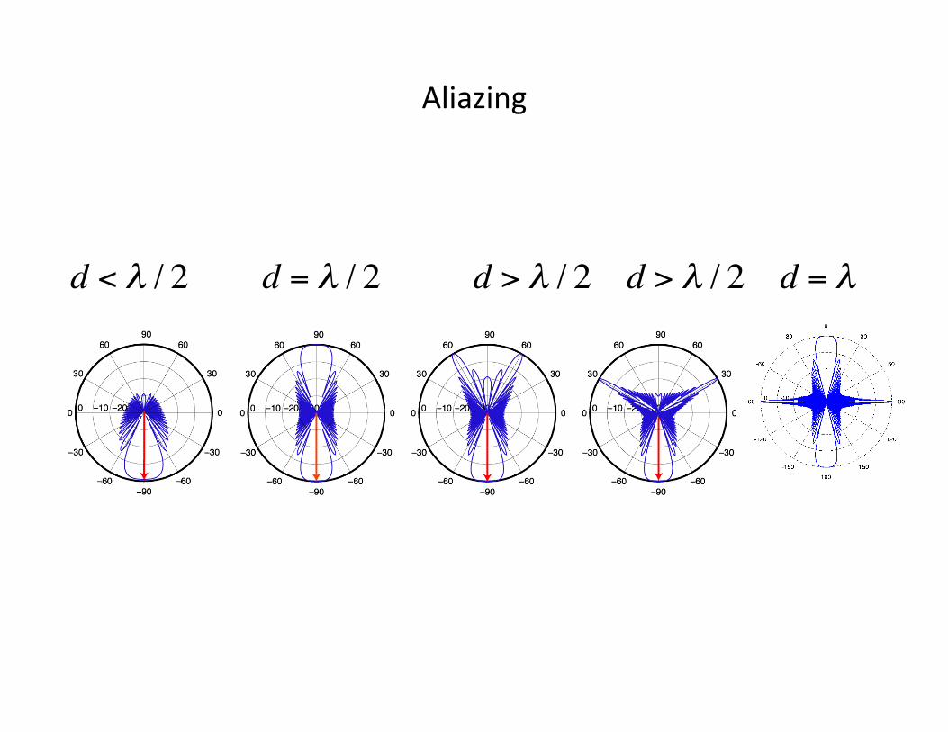
Aliazing  

d < λ / 2 d = λ / 2 d > λ / 2 d > λ / 2 d = λ

SVD  

101

Proof: Minimum Length solution

Min L(m) =mTm : d = Gm

�(m,x) =mTm+ xT (dcGm)

Lagrange multipliers leads to unconstrained minimization of

#�

#m= 2mcGTx = 0

Constrained minimization

#�

#x= dcGm = 0

�m =1

2GTx

� d = Gm =1

2GGTx

� x = 2 (GGT )c1d

�m = GT (GGT)c1d

=MX

j=1

m2j +NX

i=1

xi(di cGi,jmj)

#�

#mj= 2mj c

NX

i=1

xiGi,j

#�

#xi=

NX

i=1

(di cGi,jmj)

102

Minimum Length and least squares solutions

mML = GT (GGT )c1d

Data resolution matrix

mLS = (GTG)c1GTd

mest = Gcgd

D = GGcgdpre = Ddobs

D = G(GTG)c1GT 6= I

Least squaresMinimum length

D = GGT (GGT )c1 = I

There is symmetry between the least squares and minimum length solutions.Least squares complete solves the over-determined problem and has perfect model resolution, while the minimum length solves the completely under-determined problem and has perfect data resolution. For mix-determined problems all solutions will be between these two extremes.

R = (GTG)c1GTG = IR = GT(GGT)c1G 6= I

103

Singular value decomposition

SVD is a method of analyzing and solving linear discrete illSVD is a method of analyzing and solving linear discrete ill--posed problems. posed problems.

At its heart is the Lanczos decomposition of the matrix G

G = USV T

For a discussion see Ch. 4 of Aster et al. (2004)

G = [u1,u2, . . . ,uN ]S[v1, v2, . . . ,vM ]T

U is an N x N ortho-normal matrix with columns that span the data space

d = Gm

V is an M x M ortho-normal matrix with columns that span the model space

S is an N x M diagonal matrix with non-negative elements � singular values

UUT = UTU = IN

V V T = V TV = IM

N ×M N ×N M ×M

Ill-posed problems arise when some of the singular values are zero

Lanczos (1977)

104

S =

�

��������������

s1 0 · · · 00 s2 0 0... . . . 00 0 0 sM

0 0 0 0... ... ... ...0 0 0 0

�

��������������

It can be shown that the columns of U are the eigenvectors of the matrix GGT

Singular value decomposition

Given G, how do we calculate the matrices U, V and S ?

G = USV T

GGTui = s2i ui

It can be shown that the columns of V are the eigenvectors of the matrix GTG

GTGvi = s2i vi

The eigenvalues, si2, are the square of the elements in diagonal of the

N x M matrix S.

Try and prove this !

Try and prove this !

U = [u1|u2| . . . |uN ]

V = [v1|v2| . . . |vM ]

If N > M

S =

�

����

s1 0 · · · 0 0 · · · 00 s2 0 0 0 · · · 0... . . . 0 0 · · · 00 0 0 sN 0 · · · 0

�

����

If M > N

105

S =

�

����

s1 0 · · · 0 0 · · · 00 s2 0 0 0 · · · 0... . . . 0 0 · · · 00 0 0 sN 0 · · · 0

�

����

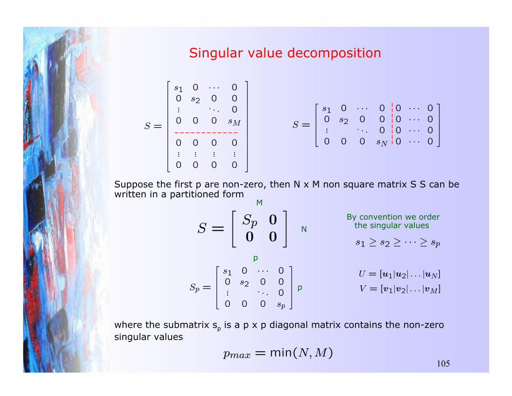
Singular value decomposition

Suppose the first p are non-zero, then N x M non square matrix S S can be written in a partitioned form

Sp =

�

����

s1 0 · · · 00 s2 0 0... . . . 00 0 0 sp

�

����

S =

"Sp 00 0

#

pmax = min(N,M)

S =

�

��������������

s1 0 · · · 00 s2 0 0... . . . 00 0 0 sM

0 0 0 0... ... ... ...0 0 0 0

�

��������������

where the submatrix sp is a p x p diagonal matrix contains the non-zero singular values

U = [u1|u2| . . . |uN ]

V = [v1|v2| . . . |vM ]

By convention we order the singular values

s1 x s2 x · · · x spN

M

p

p

106

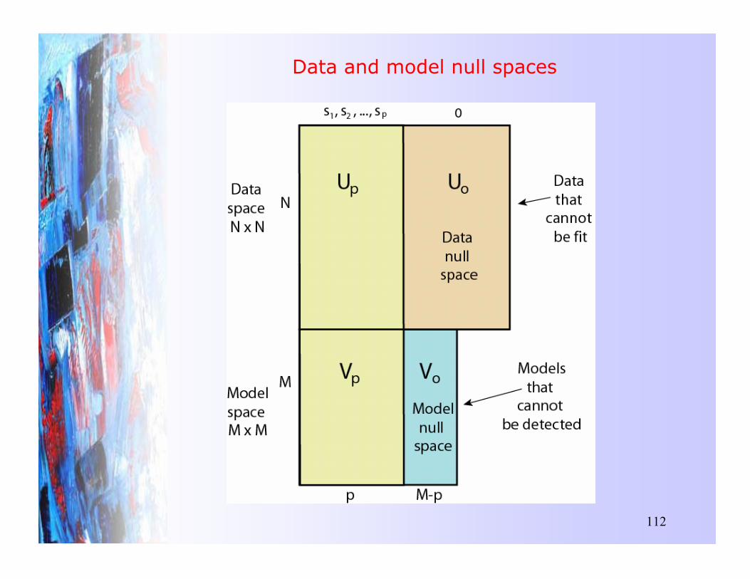
Singular value decomposition

G = [Up | Uo]"Sp 00 0

#

[Vp | Vo]T

If only the first p singular values are nonzero we write

Up represents the first p columns of UUo represents the last N-p columns ofU

Vp represents the first p columns of V

Vo represents the last M-p columns ofV

Since the columns of Vo and Uo multiply by zeros we get the compact form for G

G = UpSpVTp

� A data null space is created

� A model null space is created

Properties

UTp Uo = 0 V Tp Vo = 0 V To Vp = 0UTo Up = 0

UTp Up = I UTo Uo = I V To Vo = I V Tp Vp = I

107

Model null space

mv =MX

i=p+1

xivi

So any model of this type has no affect on the data. It lies in the model null space !

Consider a vector made up of a linear combination of the columns of Vo

Gmv =MX

i=p+1

xiUpSpVTp vi = 0

The model m lies in the space spanned by columns of Vo

Consequence: If any solution exists to the inverse problem then an infinite number will

Gmls = dobsAssume the model mls fits the data

G(mls+mv) = Gmls+Gmv

= dobs+ 0

The data can not constrain models in the model null space

Uniqueness question of Backus and Gilbert

Where have we seen this before ?

108

Example: tomography

Idealized Idealized tomographictomographic experimentexperiment

qd = Gqm

G =

�

����

G1,1 G1,2 G1,3 G1,4... ... ... ...... ... ... ...... ... ... ...

�

����

What are the entries of G ?

109

Example: tomography

Using rays 1-4

G =

�

�����

1 0 1 00 1 0 1

0S2S2 0S

2 0 0S2

�

�����

GTG =

�

����

3 0 1 20 3 2 11 2 3 02 1 0 3

�

����

This has eigenvalues 6,4,2,0.

Vp =

�

����

0.5 c0.5 c0.50.5 0.5 0.50.5 0.5 c0.50.5 c0.5 0.5

�

���� Vo =

�

����

0.50.5

c0.5c0.5

�

����

qd = Gqm

What type of change does the null space vector correspond to ?

Gvo = 0

110

Worked example: Eigenvectors

Vp =

�

����

0.5 c0.5 c0.50.5 0.5 0.50.5 0.5 c0.50.5 c0.5 0.5

�

����

Vo =

�

����

0.50.5

c0.5c0.5

�

����

S12=6 S2

2=4

S32=2 S4

2=0

112

Data and model null spaces