Efficient sampling techniques for uncertainty1

quantification in history matching using nonlinear error2

models and ensemble level upscaling techniques3

Y. Efendiev∗ A. Datta-Gupta† X. Ma‡ B. Mallick§4

Abstract5

The Markov Chain Monte Carlo (MCMC) is a rigorous sampling method to quan-6

tify uncertainty in subsurface characterization. However, the MCMC usually requires7

many flow and transport simulations in evaluating the posterior distribution and can be8

computationally expensive for fine-scale geological models. We propose a methodology9

that combines coarse- and fine-scale information to improve the efficiency of MCMC10

methods. The proposed method employs offline computations for modeling the relation11

between coarse- and fine-scale error responses. This relation is modeled using nonlinear12

statistical maps which are used in efficient sampling within MCMC framework. We13

propose two-stage MCMC where inexpensive coarse-scale simulations are performed14

to determine whether or not to run the fine-scale (resolved) simulations. The latter15

is determined based on a statistical model developed offline. The proposed method16

is an extension of the approaches considered earlier (e.g., [10]) where linear relations17

are used for modeling the response between coarse-scale and fine-scale models. The18

∗Department of Mathematics, Texas A&M University, College Station, TX 77843†Department of Petroleum Engineering, Texas A&M University, College Station, TX 77843‡Department of Petroleum Engineering, Texas A&M University, College Station, TX 77843§Department of Statistics, Texas A&M University, College Station, TX 77843

1

approach considered here does not rely on the proximity of approximate and resolved19

models and can employ much coarser and inexpensive models to guide the fine-scale20

simulations. Numerical results for three-phase flow and transport demonstrate the ad-21

vantages, efficiency and utility of the method for uncertainty assessment in the history22

matching.23

1 Introduction24

Uncertainties on the detailed description of reservoir lithofacies, porosity, and permeability25

are major contributors to uncertainty in reservoir performance forecasting. Reducing this26

uncertainty can be achieved by integrating additional data in subsurface modeling. With the27

increasing interest in accurate prediction of subsurface properties, subsurface characteriza-28

tion based on dynamic data, such as production data including gas/oil ratio becomes more29

important.30

To predict future reservoir performance, the reservoir properties, such as porosity and31

permeability, need to be conditioned to production data. It is essential that the permeability32

(and porosity) realizations adequately reflect the uncertainty in the reservoir properties, i.e.,33

the probability distribution is sampled correctly. The uncertainty quantification is typically34

carried out in a Bayesian framework where multiple realizations are sampled from a posterior35

distribution that incorporates the prior information (e.g., [18]). This problem is challenging36

because the permeability field is a function defined on a large number of grid blocks and37

the production data nonlinearly depends on permeability. The Markov Chain Monte Carlo38

(MCMC) method and its modifications have been used in previous findings to sample the39

posterior distribution (e.g., [24]).40

The direct MCMC simulations are generally very CPU demanding because each proposal41

requires solving a forward coupled nonlinear partial differential equations over a large time42

interval. The forward fine-scale problem is usually formulated on a large number of grid43

2

blocks, which makes it prohibitively expensive to perform sufficient number of MCMC sim-44

ulations. There have been a few attempts to propose MCMC methods with high acceptance45

rate (e.g., [18, 24, 25]). For example, the randomized maximum likelihood method uses46

unconditional realizations of the production and permeability data and solves a determin-47

istic gradient-based inverse problem. The solution of this minimization problem is taken48

as a proposal, and is accepted with probability one, because the rigorous acceptance prob-49

ability is very difficult to estimate. Though efficient in many cases, this method may not50

properly sample the posterior distribution [22]. Thus, developing efficient rigorous MCMC51

calculations with high acceptance rate remains a challenging problem.52

In this paper, we extend two-stage MCMC methods considered before (e.g., [10, 11]).53

The two-stage MCMC involves a pre-screening stage where the proposals are screened using54

approximate models. If the proposal is accepted in the first stage (screening stage), then the55

resolved computations are performed to compute the acceptance probability. The novelty56

of the proposed approach is two-fold. First, we employ error modeling ([16, 28, 15, 4,57

26, 20]) which allows mapping the coarse-scale data to the fine-scale data via a nonlinear58

map. The main goal of the error modeling is to construct a map from the coarse-scale59

errors between computed and observed data to the fine-scale errors based on some prior60

(offline) computations. The mapping between these low dimensional quantities is often61

easy to construct based on fewer samples. Secondly, we consider inexpensive ensemble level62

upscaling type methods for coarse-scale modeling (cf. [2]). To our best knowledge the error63

models have not yet been used in rigorous sampling methods. Previous approaches within64

two-stage MCMC methods [11, 10] have used only linear relation between coarse- and fine-65

scale responses. Though it is found to be effective in many cases, linear relations may not be66

very reliable when coarse-scale models both across spatial scales and uncertainties (in highly67

nonlinear equations) are considered. In particular, for the examples presented here we have68

found poor performance when linear models are used.69

3

Ensemble level upscaling methods compute upscaled quantities which represent not only70

subgrid variations, but also variations across the ensemble. These approaches compute71

upscaled coefficients based on some sampled realizations. In this paper, we use some se-72

lected realizations based on the idea of sparse interpolation techniques to compute reference73

points for upscaled permeabilities. Furthermore, for an arbitrary realization, the upscaled74

permeability is interpolated using the pre-computed values of upscaled permeabilities at ref-75

erence points. This procedure saves the computational time by avoiding the computation76

of upscaled quantities. Though for upscaled permeabilities such a saving may not be very77

important, for the computations of pseudo relative permeabilities or when using global up-78

scaling methods, these computational saving is important. We note that one can consider79

more general ensemble level upscaling methods such as those presented in [2].80

Two-stage MCMC methods considered here modifies the instrumental probability dis-81

tribution by filtering the proposals via simplified models. Our numerical results show that82

using inexpensive coarse-scale computations one can increase the acceptance rate of MCMC83

calculations. Here the acceptance rate refers to the ratio between the number of accepted84

permeability samples and the number of times of solving the fine-scale nonlinear PDE system.85

In offline computational stage, we use several hundreds realizations of the permeability field86

to construct an error model and develop ensemble level upscaling. For the error modeling,87

we use piece-wise linear functions to fit the scattered data representing coarse-scale errors vs.88

fine-scale errors. At the first stage, using coarse-scale runs we determine whether or not to89

run the fine-scale simulations. To compute the approximation of the fine-scale error, offline90

statistical models are used. If the proposal is accepted at the first-stage, then a fine-scale91

simulation is performed at the second stage to determine the acceptance probability of the92

proposal. The first stage of the MCMC method modifies the proposal distribution. It is easy93

to show that the modified Markov chain satisfies the detailed balance condition for the cor-94

rect distribution. In the paper, we also discuss the efficiency of two-stage MCMC methods.95

4

We would like to note that two-stage MCMC algorithms have been used previously (e.g.,96

[3, 19, 26, 17]) in different situations.97

Numerical results for permeability fields generated using two-point geostatistics are pre-98

sented in the paper. Using the Karhunen-Loeve expansion, we can represent the high dimen-99

sional permeability field by a number of parameters. Furthermore, static data (the values of100

permeability field at some sparse locations) can be easily incorporated into the Karhunen-101

Loeve expansion to further reduce the dimension of the parameter space. Numerical results102

are presented for black oil model (three phase flow and transport) with 8 production wells103

and 1 injection well. In all the simulations, we observe nearly two times increase in the104

acceptance rate. In other words, the preconditioned MCMC method can accept the same105

number of samples with much less fine-scale runs.106

The paper is organized in the following way. In the next section, we briefly describe107

the model equations and their upscaling. Section 3 is devoted to the description of MCMC108

methods. Numerical results are presented in Section 4.109

2 Fine and coarse models110

In this section we briefly introduce the fine- and coarse-scale models used in the simulations.111

We consider black oil model in a subsurface formation (denoted by Ω) under the assumption112

that the displacement is dominated by viscous effects. We neglect the effects of gravity and113

capillary pressure, although our proposed approach is independent of the choice of physical114

mechanisms. Porosity will be considered to be constant. The phases will be referred to as115

water, oil and gas, designated by subscripts w, o, and g, respectively. Simultaneous flow of116

three phases is governed by the following three equations (e.g., [5])117

∂

∂t

(

Sj

Bj

)

+ ∇ ·(

k(x)krj

µjBj∇pj

)

= qsj , j = w, o, (1)

5

∂

∂t

(

Sg

Bg+

SoRso

Bo

)

+ ∇ ·(

k(x)kroRso

µoBo∇po +

k(x)krg

µgBg∇pg

)

= qsg, (2)

where Bj (j = w, o) is the formation volume factor of phase j, k(x) is heterogeneous absolute118

permeability field, qs is the source terms, pj is the pressure of the phase j, krj is the relative119

permeabilities, Sj is the saturation of the phase j and Rso is the solubility of gas in oil.120

Next, we will briefly describe single-phase flow upscaling procedure. These types of121

approaches for upscaling are discussed by many authors; see e.g., [9]. The main idea of this122

approach is to upscale the absolute permeability field k(x) on the coarse-grid (see Figure 1),123

then solve the original system on the coarse-grid with upscaled permeability field. Below, we124

discuss briefly the upscaling of absolute permeability and ensemble level upscaling methods125

used in our simulations.126

Consider the fine-scale permeability that is defined in the domain with underlying fine127

grid as shown in Figure 1. On the same graph we illustrate a coarse-scale partition of the128

domain. To calculate the upscaled permeability field at the coarse-level, we use the solutions129

of local pressure equations. The main idea of the calculation of a coarse-scale permeability130

is that it delivers the same average response as that of the underlying fine-scale problem131

locally. For each coarse domain K, we solve the local problems132

div(k(x)∇φj) = 0, (3)

with some coarse-scale boundary conditions. Here k(x) denotes the fine-scale permeability133

field. We will use the boundary conditions which are given by φj = 1 and φj = 0 on the134

opposite sides along the direction ej and no flow boundary conditions on all other sides. For135

these boundary conditions, the coarse-scale permeability tensor is given by136

(k∗ej , el) =1

|K|

∫

K

(k(x)∇φj(x), el)dx, (4)

6

where φj is the solution of (3) with prescribed boundary conditions. Various boundary137

condition can have some influence on the accuracy of the calculations, including periodic,138

Dirichlet and etc. These issues have been discussed in e.g., [30]. In particular, for determining139

the coarse-scale permeability field one can choose the local domains that are larger than140

the target coarse block, K, for (3). Once the upscaled absolute permeability is computed,141

the original equation is solved on the coarse-grid, without changing the form of relative142

permeability curves.143

Ensemble level upscaling methods compute the upscaled permeabilities based on values144

of upscaled permeability fields for some realizations which are computed offline. To demon-145

strate the concept, we assume that the permeability field is computed for realizations ω1,146

..., ωN and the values are k∗(x, ω1), ..., k∗(x, ωN). In general, ω is infinite dimensional,147

though in applications considered in this paper, the permeability fields are characterized by148

two-point correlation functions on a fine grid and ω will be taken to be finite dimensional.149

Ensemble level upscaling attempts to approximate k(x, ω) for any value of ω using k∗(x, ω1),150

..., k∗(x, ωN). First work in this direction ([2]) uses statistical approach for this approxima-151

tion. In this paper, we employ deterministic interpolation theory to approximate k∗(x, ω)152

given k∗(x, ω1), ..., k∗(x, ωN). In our simulations, we will be using linear relations for log of153

permeabilities and sparse interpolation techniques in high dimensional space (e.g., [31]) to154

approximate k∗(x, ω). In particular,155

log(k∗(x, ω)) =∑

i

Li(ω) log(k∗(x, ωi)),

where Li(ω) are interpolation weights which are readily available for interpolations considered156

here.157

As for the quantities which will be used to condition the permeability field, we take158

gas/oil ratio (commonly abbreviated GOR). When oil is brought to surface conditions it is159

7

usual for some gas to come out of solution. GOR is the ratio of the gas that comes out of the160

solution, to the volume of oil. Our goal in this paper, is to sample the fine-scale permeability161

field based on GOR which is a function of time in each producing well. The relation between162

GOR and the permeability field is highly nonlinear and can not be accurately described via163

linear relations.164

3 Methodology165

To find the permeability field given GOR information, we assume that an observed GOR,166

F ref(t), is given. Consequently, one can consider this problem as a sampling from the167

conditional distribution P (k|F ref). Using Bayes theorem we can write168

P (k|F ref) ∝ P (F ref |k)P (k). (5)

The normalizing constant in this expression is not important, because we use iterative updat-169

ing procedure. In (5), P (F ref |k) represents the likelihood function and requires the forward170

solution of black oil model. We will be using Metropolis-Hasting MCMC (see [27]) to sample171

from the posterior distribution P (k|F ). The main idea of MCMC is to generate a Markov172

chain whose stationary distribution is given by P (k|F ref). At each iteration, a permeability173

field, k, is proposed using instrumental distribution q(k|kn) (where kn is previously accepted174

permeability field), and then forward problem is solved to determine the acceptance proba-175

bility,176

Pr(kn, k) = min

(

1,q(kn|k)P (k|F ref)

q(k|kn)P (kn|F ref)

)

, (6)

i.e. kn+1 = k with probability Pr(kn, k), and kn+1 = kn with probability 1 − Pr(kn, k).177

Since each proposal requires the fine-scale computation, direct (full) MCMC is expensive.178

Typically, direct MCMC requires many iterations for the convergence to a steady state, where179

8

each iteration involves the computation of the fine-scale solution over a large time interval.180

One way to achieve efficiency is to propose an algorithm that increases the acceptance rate of181

MCMC. This minimizes rejection of proposals after detailed flow and transport calculations.182

In this paper, we use coarse-scale solutions based on single-phase upscaling to increase the183

acceptance rate. The main idea of this algorithm is to compare GOR that correspond to the184

coarse-scale models to determine whether or not to run fine-scale simulations.185

To formulate the algorithm, we introduce several notations. For our numerical results,186

we will sample the likelihood187

π(k) = P (F ref |k) ∝ exp(−‖F ref − Fk‖2

σf), (7)

where F ref is GOR, Fk is GOR that is obtained from the simulations with permeability k,188

and Σ = σfI is covariance matrix representing the measurement errors. Here ‖F ref −Fk‖ =189

(

∫ T

0|F ref − Fk|2dt

)1/2

is the fine-scale error between the simulated and the observed data.190

We note that GOR is a function of time at producing wells. In our simulations, we start191

with a number of realizations (usually 100-200) of the permeability field and construct the192

error model between ‖Fk − F ref‖ and ‖Fk∗ − F ref‖ (see Figure 7). Using known statistical193

methods we derive nonlinear relation between these quantities194

‖Fk − F ref‖ ≈ G(‖Fk∗ − F ref‖),

where G is a nonlinear function which is estimated based on a limited number of realizations195

of the permeability field. G can be assumed to be random as it is done in our simulations.196

In our simulations, we use piece-wise Gaussian processes to fit the relation ‖Fk − F ref‖ vs.197

‖Fk∗ − F ref‖. In this case, the surrogate probability distribution used in the simulations is198

π∗(k) = P (F ref |k∗) ∝ exp(− 1

σf

G0(‖Fk∗ − F ref‖)σk∗

),

9

where G0 and σk∗ are the mean and the variance of the piece-wise Gaussian for a given k∗199

(see Figure 7). The subscript k∗ is used in σ to indicate that the variance of piece-wise200

Gaussian model is a function of k∗. We note that one can use more general probabilistic201

models to model error relations and also use the full covariance matrix corresponding to the202

measurement errors.203

Algorithm (two-stage MCMC with nonlinear error model)204

• Offline: Start with offline computations of GOR cross-plot by computing ‖Fk −F ref‖205

and ‖Fk∗ −F ref‖. Estimate the operator G, such that ‖Fk −F ref‖ ≈ G(‖Fk∗ −F ref‖).206

• Offline: Compute k∗(x, ωi) for some realizations ωi.207

• Step 1. At kn generate k from q(k|kn).208

• Step 2. Accept k for the fine-scale run with probability209

g(kn, k) = min

(

1,q(kn|k)π∗(k)

q(k|kn)π∗(kn)

)

, (8)

i.e. kn+1 = k (conditionally) with probability h(kn, k), and kn+1 = kn (conditionally)210

with probability 1 − g(kn, k). If rejected go to step 1.211

• Step 3. Accept k with probability212

Pr(kn, k) = min

(

1,Q(kn|k)π(k)

Q(k|kn)π(kn)

)

, (9)

i.e. kn+1 = k with probability Pr(kn, k), and kn+1 = kn with probability 1−Pr(kn, k).213

The proposal function Q(k|kn) satisfies214

Q(k|kn) = g(kn, k)q(k|kn) +

(

1 −∫

g(kn, k)q(k|kn)dk

)

δkn(k). (10)

10

The expression for Q can be simplified (e.g., [11])215

Pr(kn, k) = min

(

1,π(k)π∗(kn)

π(kn)π∗(k)

)

. (11)

One can also add new data to improve the estimates; however, this can introduce bias and216

will be avoided in our simulations.217

In [11], it was shown that the detailed balance condition holds and MCMC converges to218

the correct distribution. This proof applies here. We would like to note that from (11) one219

obtains (see [10, 11]) that220

Pr(kn, k) > exp

−‖Fk − F ref‖ − G0(‖Fk∗−F ref‖)

σk∗

σf

+‖Fkn

− F ref‖ − G0(‖Fk∗n−F ref‖)

σk∗

σf

.

It is clear from this expression that if the error in ‖Fk − F ref‖ − G0(‖Fk∗ − F ref‖)/σk∗ is221

small for a generic k, the acceptance probability is close to 1. Thus, if the approximation222

with G is accurate and the spread of this approximation is low, then one can achieve high223

acceptance rate. Clearly, if the coarse-scale model approximates the results of the fine-scale224

simulations, then one can achieve high acceptance rate. However, in general, single-phase225

upscaling techniques do not provide accurate approximations of the fine-scale results for226

three-phase systems and thus modeling the relation between coarse- and fine-scale models227

are needed. The errors associated with this modeling will affect the efficiency of two-stage228

MCMC methods. In this paper, we explore this via numerical simulations.229

We again note this approach extends previous approaches within two-stage MCMC meth-230

ods [11, 10] where linear relations between coarse- and fine-scale responses are used. In the231

numerical examples considered in this paper, we have found poor performance when linear232

models are used.233

11

4 Numerical results234

For our numerical tests, we use the Karhunen-Loeve expansion (KLE) [21, 29] to obtain the

permeability field in terms of an optimal L2 basis. By truncating KLE, we can represent

the permeability matrix by a small number of random parameters. To impose the hard

constraints (the values of the permeability at prescribed locations), one can find a linear

subspace of our parameter space (a hyperplane) which yields the corresponding values of

the permeability field. First, we briefly recall the facts of the KLE. Denote Y (x, ω) =

log[k(x, ω)], where the random element ω is included to remind us that k is a random field.

We assume that E[Y (x, ω)] = 0. Suppose Y (x, ω) is a second order stochastic process with

E∫

ΩY 2(x, ω)dx < ∞, where E is the expectation operator. Given an orthonormal basis

φk in L2(Ω), we can expand Y (x, ω) as

Y (x, ω) =∞

∑

k=1

Yk(ω)φk(x), Yk(ω) =

∫

Ω

Y (x, ω)φk(x)dx.

We are interested in the special L2 basis φk which makes the random variables Yk un-

correlated. That is, E(YiYj) = 0 for all i 6= j. Denote the covariance function of Y as

R(x, y) = E [Y (x)Y (y)]. Then such basis functions φk satisfy

E[YiYj] =

∫

Ω

φi(x)dx

∫

Ω

R(x, y)φj(y)dy = 0, i 6= j.

Since φk is a complete basis in L2(Ω), it follows that φk(x) are eigenfunctions of R(x, y):235

∫

Ω

R(x, y)φk(y)dy = λkφk(x), k = 1, 2, . . . , (12)

12

where λk = E[Y 2k ] > 0. Furthermore, we have236

R(x, y) =∞

∑

k=1

λkφk(x)φk(y). (13)

Denote ηk = Yk/√

λk, then ηk satisfy E(ηk) = 0 and E(ηiηj) = δij . It follows that237

Y (x, ω) =∞

∑

k=1

√

λkηk(ω)φk(x), (14)

where φk and λk satisfy (12). We assume that the eigenvalues λk are ordered as λ1 ≥ λ2 ≥ . . ..238

The expansion (14) is called the Karhunen-Loeve expansion. In the KLE (14), the L2 basis239

functions φk(x) are deterministic and resolve the spatial dependence of the permeability field.240

The randomness is represented by the scalar random variables ηk.241

After we discretize the domain Ω by a rectangular mesh, the continuous KLE (14) is

reduced to a finite number of terms. In our paper, we work with finite dimensional covariance

matrices defined over the square domain with 50 × 50 resolution. As a consequence, the

covariance matrix is 2500 × 2500. Note that we only need to keep the leading order terms

(quantified by the magnitude of λk) and still capture most of the energy of the stochastic

process Y (x, ω). For an N -term KLE approximation YN =∑N

k=1

√λkηkφk, define the energy

ratio of the approximation as

e(N) :=E‖YN‖2

E‖Y ‖2=

∑Nk=1 λk

∑∞k=1 λk

.

If λk, k = 1, 2, . . . , decay very fast, then the truncated KLE would be a good approximation242

of the stochastic process in the L2 sense.243

It is common to use variogram instead of covariance functions for stochastic permeability244

fields. The relation between them can be easily written as γ(x, y) = C − R(x, y), where245

C = E(Y (x, ω)2) is constant for stationary processes and γ(x, y) denotes the variogram.246

13

Typical variograms used in the modeling of subsurface processes are exponential, normal,247

and spherical [6]. In this paper, we will use spherical variogram and denote correlation248

lengths by l1, l2 and the variance of log(k) by σlog(k). We first solve the eigenvalue problem249

(12) numerically on the rectangular mesh and obtain the eigenpairs λk, φk. Further, we250

can sample Y (x, ω) from the truncated KLE (14) by generating Gaussian random variables251

ηk.252

In all numerical simulations, we will assume that the reservoir is filled with oil and water253

is injected to displace the oil. We consider 9 spot pattern of water flooding. There is one254

water injector, and 8 producers (see Figure 2). The domain is taken to be square with255

50× 50 fine grid resolution with dimensions 50× 50. The coarse grid is taken to be uniform256

5×5 in all cases. As for ensemble level upscaling, we use lowest order Smolyak interpolation257

which provides 2d + 1 nodes in d-dimensional space. We refer to [31] for the description of258

Smolyak interpolation and to [7] the results on upscaling using Smolyak interpolation. As259

we mentioned earlier that ensemble level upscaling techniques used here simply interpolate260

the log of upscaled permeability based on the values of log of upscaled permeability at some261

regularly spaced points in high dimensions. Because the points are regularly spaced the262

interpolation formula and interpolation weights can be easily derived (see [31]).263

Solution gas/oil ratio and gas formation volume factor are shown in Figure 3 (left) and264

Figure 3 (right). From right top figure, the bubble point pressure of the reservoir is 3000265

psia. Relative permeability of water, oil, and gas are shown in Figure 4 (left) and in Figure266

4 (right). Modified Stones II second three-phase relative permeability model was used to267

compute oil relative permeability [1]. We note that if reservoir pressure is above the bubble268

point pressure, the flow is two-phase (water and oil); if the pressure drops below the bubble269

point pressure, then the gas evolves into a liquid phase and a gas phase. The flow is three-270

phases: water, oil and gas. There are maximum of three components, water, oil and gas.271

In the black oil model, it is assumed that no mass transfer occurs between the water phase272

14

and other two phases. Moreover, the mass fractions of the oil and gas components in the oil273

phase can be determined by gas solubility.274

In the first example, we use a reference permeability field with the correlation lengths275

lx = 30, ly = 2, and the variance of log(k) is 2. A realization of this permeability field is276

used to generate a reference permeability field. In the sampling procedure, we choose the277

permeability fields with different correlation lengths (still on 50 × 50 fine grid resolution).278

In particular, we choose lx = 18, ly = 3 and keep only 50 eigenvalues/eigenvectors in KLE.279

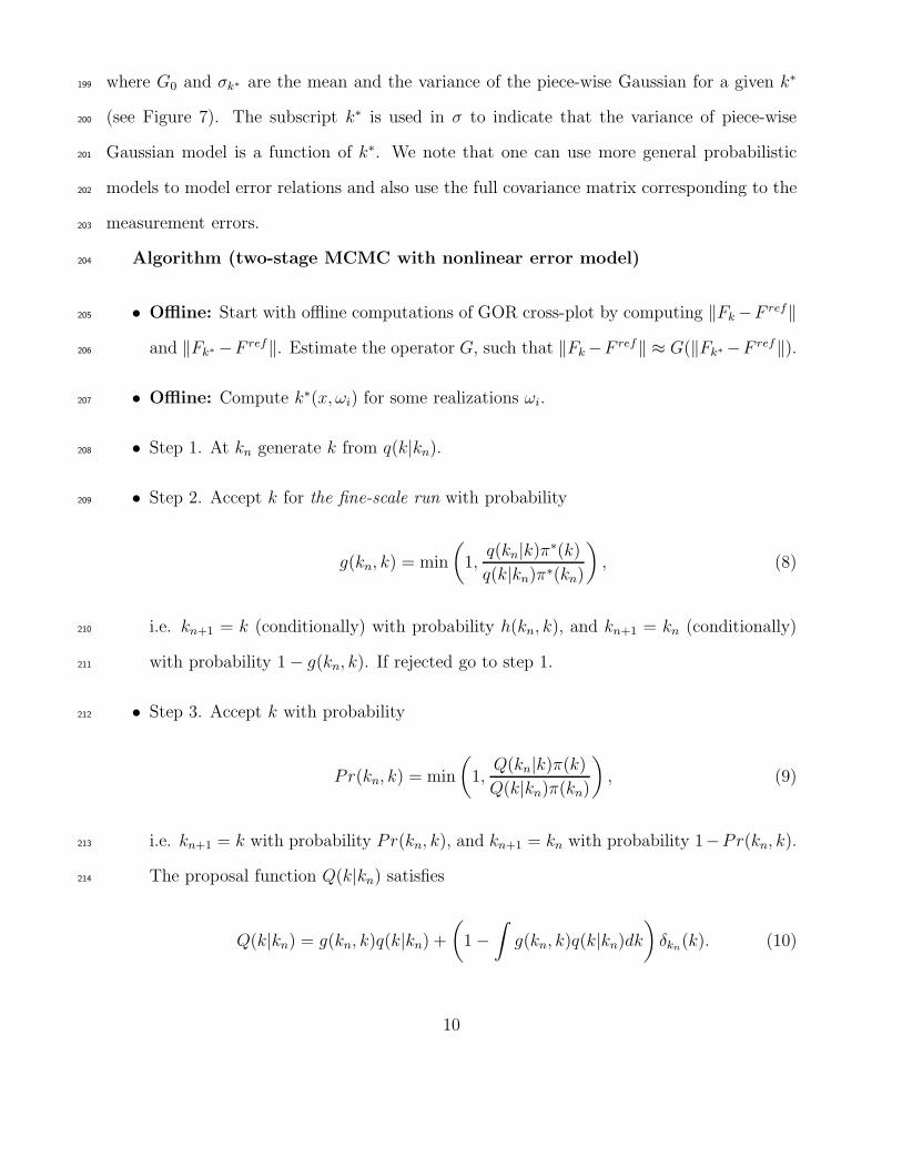
In Figure 5, GOR misfit vs. iterations are plotted. We compare the use of two coarse scale280

models. In the first case, we use the coarse-scale model where no approximation is made in281

computing upscaled permeabilities. In the second example, we use ensemble level upscaled282

permeability which is computed based on offline computations. We note that the second283

case is less accurate though less expensive to compute. We observe from this figure that284

all three curves show that the two-stage MCMC methods have similar convergence as the285

full MCMC. These results are based on 1000 proposals. The acceptance rates are given286

as following, full MCMC - 8.8 %, two-stage MCMC with upscaling is 22 %, and two-stage287

MCMC with ensemble level upscaling is 17 %. We observe that two-stage MCMC methods288

provide nearly two times higher acceptance rates. Since the computational cost associated289

with coarse-scale simulations is negligble, two-stage MCMC methods improve CPU required290

for sampling the posterior distribution by nearly two-fold. In all simulations, random walk291

instrumental distribution for q(k|kn) is used, where k = kn + ǫn with ǫn being a random292

perturbation with prescribed distribution. The formal convergence diagnosis can performed293

using multiple chains method based convergence diagnosis ([14]). In this paper, our goal is294

to compare modified chain with the chain obtained via direct MCMC, and thus we restrict295

ourselves to only showing RMS vs. the number of iterations. We note that the convergence296

diagnostics has nothing to do with the rate of convergence, which depends on the second297

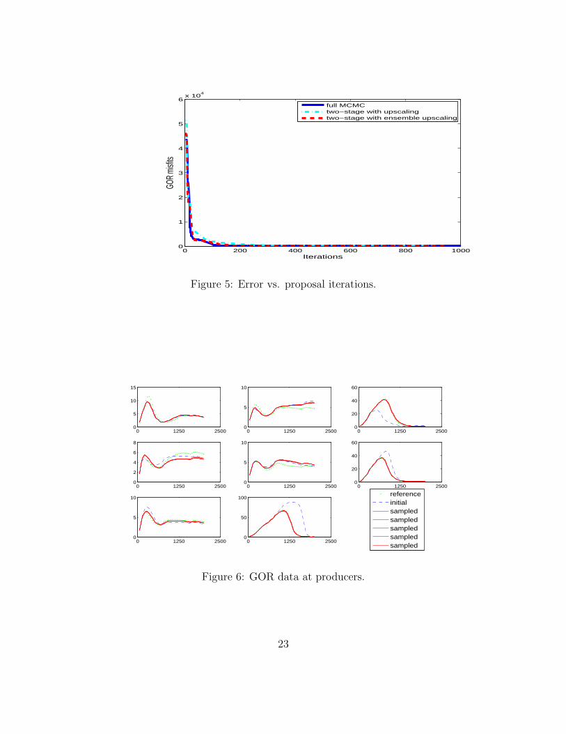
largest eigenvalue of the transition matrix of the Markov chain. Figure 6 shows the GOR298

15

matches of the producers. As we see that the sampled realizations match GOR very well.299

In these figures, reference GOR is designated by green color, and initial GOR is designated300

by blue, and the sampled GORs are designated by red color. The data which is used to301

model the error is presented in Figure 7. We plot both mean as well as mean plus/minus302

standard deviation. In our simulations, we have used piecewise linear relation to model the303

mean behavior and constant variation within each bin. Furthermore, Gaussian distribution304

is used for each bin. In Figure 8, the samples of the permeability field are depicted. One305

can observe that the initial model does not have the high flow channel located at upper side306

of the domain, while the corrected permeability models have this high conductivity region.307

In the second example, the reference permeability field is chosen with the correlation308

lengths lx = 25 and ly = 6 and 100 eigenvalues/eigenvectors are kept in KLE. For sampling309

purposes, the permeability fields are generated with 50× 50 fine resolution and with lx = 20310

and lz = 4 and 40 eigenvalues/eigenvectors are kept in KLE. In Figure 9, GOR misfit vs.311

iterations are plotted. As before, we compare the use of two coarse scale models. In the312

first case, we use coarse-scale model where no approximation is made in computing upscaled313

permeabilities. In the second example, we use ensemble level upscaled permeability which is314

computed based on offline computations. We observe from this figure that all three curves315

show that the two-stage MCMC has similar convergence as the full MCMC. These results316

are based on 1000 proposals. The acceptance rates are given as following, full MCMC -317

12 %, two-stage MCMC with upscaling is 24 %, and two-stage MCMC with ensemble level318

upscaling is 20 %. Figure 10 shows the GOR matches of the producers. As we see that319

the sampled realizations match GOR very well. As before, reference GOR is designated by320

green color, and initial GOR is designated by blue, and the sampled GORs are designated321

by red color. The data which is used to model the error is presented in Figure 11. In our322

simulations, we have used piecewise linear relation to model the mean behavior and constant323

variation within each segment.324

16

5 Conclusions325

In this paper, we study two-stage MCMC methods which use simplified and inexpensive326

upscaled models to speed-up the sampling of the posterior distribution. Our underlying327

equations describe the flow and transport of three-phase flow system in heterogeneous porous328

media. We employ single-phase upscaling methods for coarsening the flow and transport329

equations. Because single-phase upscaling techniques are not very accurate for complex black330

oil models (see e.g., Figure 11), the proposed algorithm requires offline computations where331

a nonlinear relation between the coarse- and fine-scale models are constructed. This relation332

is used within the context of two-stage MCMC to perform rigorous sampling. The proposed333

method generalizes the existing multi-stage MCMC methods where a linear relation between334

coarse- and fine-scale models are used. In our coarse-scale models, we also use ensemble level335

upscaling techniques for inexpensive coarse-scale computations. The efficiency of two-stage336

MCMC methods depends on the accuracy of the nonlinear approximation and the spread in337

this approximation. The modeling errors in this approximation affect the efficiency of two-338

stage MCMC methods. In this paper, we explore this via numerical simulations. Numerical339

results study the advantages, efficiency and utility of the method for uncertainty assessment340

in the history matching. We show that two-stage MCMC methods provide two times higher341

acceptance rates, and thus improve CPU required for sampling the posterior distribution by342

nearly two-fold.343

References

[1] K. Aziz, Petroleum reservoir simulation, Chapman & Hall, 1979.

[2] Y. Chen and L. Durlofsky, An ensemble level upscaling approach for efficient

estimation of fine-scale production statistics using coarse-scale simulations, SPE paper

17

106086, presented at the SPE Reservoir Simulation Symposium, Houston, Feb. 26-28

(2007).

[3] A. Christen and C. Fox, MCMC using an approximation, Technical report, Depart-

ment of Mathematics, The University of Auckland, New Zealand.

[4] M. Christie, J. Glimm, J. Grive, D. Highon, D. Sharp, and M. Wood-

Schultz, Error analysis ans simulations of complex phenomena, Los Alamos Sci. 29

(2005) 625.

[5] A. Datta-Gupta and M.J. King, Streamline Simulation: Theory and Practice, Pub-

lisher: Society of Petroleum Engineers, 2007

[6] C. V. Deutsch and A. G. Journel, GSLIB: Geostatistical software library and

user’s guide, 2nd edition, Oxford University Press, New York, 1998.

[7] P. Dostert, Uncertainty Quantification Using Multiscale Methods for Porous Media

Flows, Ph.D. thesis, Texas A&M University, 2007

[8] P. Dostert, Y. Efendiev, T. Hou, and W. Luo, Coarse-gradient Langevin algo-

rithms for dynamic data integration and uncertainty quantification, 217 (1), pp.123-142,

2006

[9] L. J. Durlofsky, Numerical calculation of equivalent grid block permeability tensors

for heterogeneous porous media, Water Resour. Res., 27 (1991), pp. 699–708.

[10] Y. Efendiev, A. Datta-Gupta, V. Ginting, X. Ma, and B. Mallick, An

efficient two-stage Markov chain Monte Carlo method for dynamic data integration, 41,

W12423, doi:=10.1029/2004WR003764

[11] Y. Efendiev, T. Hou and W. Luo, Preconditioning Markov chain Monte Carlo

simulations using coarse-scale models, SIAM. Sci. Comp. 28(2), pp. 776-803.

18

[12] V. Ginting, Analysis of two-scale finite volume element method for elliptic problem,

Journal of Numerical Mathematics, 12(2) (2004), pp. 119–142.

[13] P. Frauenfelder, C. Schwab and R. A. Todor, Finite elements for elliptic

problems with stochastic coefficients, Comput. Methods Appl. Mech. Engrg., 194 (2005),

pp. 205–228.

[14] Gelman, A., and Rubin, B., 1992, Inference from iterative simulation using multiple

sequences , Statistical Science, 7, pp. 457-511.

[15] J. Glimm and D. H. Sharp, Prediction and the quantification of uncertainty, Phys. D,

133 (1999), pp. 152–170. Predictability: quantifying uncertainty in models of complex

phenomena (Los Alamos, NM, 1998).

[16] J. Glimm, S. Hou, Y.H. Yee, D.H. Sharp and K. Ye, Solution error models for

uncertainty quantification, AMS Advances in Differential Equations and Mathematical

Physics (2002).

[17] D. Higdon, H. Lee and Z. Bi, A Bayesian approach to characterizing uncertainty in

inverse problems using coarse and fine-scale information, IEEE Transactions on Signal

Processing, 50(2) (2002), pp. 388-399.

[18] P. Kitanidis, Quasi-linear geostatistical theory for inversing, Water Resour. Res., 31

(1995), pp. 2411–2419.

[19] J. S. Liu, Monte Carlo Strategies in Scientific Computing, Springer, New-York, 2001.

[20] O. Lodoen, H. Omre, L. Durlofsky, and Y. Chen, Assessment of uncertainty

in reservoir production forecasts using upscaled models, in proceedings of the 7th Inter-

national Geostatistics Congress, Banff, Canada, September 26 - October 1, 2004.

[21] M. Loeve, Probability Theory, 4th ed., Springer, Berlin, 1977.

19

[22] X. Ma, M. Al-Harbi, A. Datta-Gupta, and Y. Efendiev An Efficient Two-

Stage Sampling Method for Uncertainty Quantification in History Matching Geological

Models, to appear in SPEJ.

[23] S. P. Meyn, R. L. Tweedie, Markov Chains and Stochastic Stability, Springer-Verlag,

London, 1996.

[24] D. Oliver, L. Cunha, and A. Reynolds, Markov chain Monte Carlo methods for

conditioning a permeability field to pressure data, Mathematical Geology, 29 (1997).

[25] D. Oliver, N. He, and A. Reynolds, Conditioning permeability fields to pressure

data, 5th European conference on the mathematics of oil recovery, Leoben, Austria, 3-6

September, 1996.

[26] H. Omre and O. P. Lodoen, Improved production forecasts and history matching

using approximate fluid flow simulators, SPE Journal, September 2004, pp. 339-351.

[27] C. Robert and G. Casella, Monte Carlo Statistical Methods, Springer-Verlag, New-

York, 1999.

[28] A. O′Sullivan, Modelling Simulation Error For Improved Reservoir Prediction, PhD

Thesis, (Heriot Watt University, 2004).

[29] E. Wong, Stochastic Processes in Information and Dynamical Systems, MCGraw-Hill,

1971.

[30] X. H. Wu, Y. Efendiev, and T. Y. Hou, Analysis of upscaling absolute permeabil-

ity, Discrete and Continuous Dynamical Systems, Series B, 2 (2002), pp. 185–204.

[31] D. Xiu and J. Hesthaven, High-Order Collocation Methods for Differential Equations

with Random Inputs, SIAM J. Sci. Comput. Wol. 27, No. 3, 2007, pp. 1118-1139.

20

Coarse−grid Fine−grid

K

Figure 1: Schematic description of fine- and coarse-grids. Bold lines illustrate a coarse-scalepartitioning, while thin lines show a fine-scale partitioning within coarse-grid cells.

injectorproducer

Figure 2: Well configuration used in the simulations.

21

0 2000 4000 6000 8000 100000

20

40

60

80

100

120

140

160

180

Pressure, psia

Ga

s F

VF

RB

/Mscf

0 2000 4000 6000 8000 100000

0.2

0.4

0.6

0.8

1

1.2

1.4

Pressure, psia

So

lutio

n G

as/O

il R

atio

Mscf/

ST

B

Figure 3: Solution gas/oil ratio and gas formation volume factor.

0 0.2 0.4 0.6 0.80

0.1

0.2

0.3

0.4

0.5

0.6

0.7

0.8

0.9

1

Sw

Re

lative

Pe

rme

ab

ility

krwkrow

0 0.1 0.2 0.3 0.4 0.50

0.1

0.2

0.3

0.4

0.5

0.6

0.7

0.8

0.9

1

Sg

Re

lative

Pe

rme

ab

ility

krgkrog

Figure 4: Relative permeabilities used in the simulations.

22

0 200 400 600 800 10000

1

2

3

4

5

6x 10

4

Iterations

GOR

misfi

ts

full MCMCtwo−stage with upscalingtwo−stage with ensemble upscaling

Figure 5: Error vs. proposal iterations.

0 1250 25000

5

10

15

0 1250 25000

5

10

0 1250 25000

20

40

60

0 1250 25000

2

4

6

8

0 1250 25000

5

10

0 1250 25000

20

40

60

0 1250 25000

5

10

0 1250 25000

50

100

referenceinitialsampledsampledsampledsampledsampled

Figure 6: GOR data at producers.

23

0 2 4 6 8 10

x 104

−0.5

0

0.5

1

1.5

2

2.5

3x 10

5

Coarse

Fine

mean+stdmean−stdmeandata

Figure 7: Error model.

Reference Initial Sample 1

Sample 2 Sample 3 Sample 4

200

400

600

800

1000

Figure 8: Permeability realizations.

24

0 200 400 600 800 10000

1000

2000

3000

4000

5000

6000

7000

8000

9000

full MCMCtwo−stage with upscalingtwo−stage with ensemble upscaling

Figure 9: Error vs. proposal iterations.

0 1250 25000

5

10

0 1250 25000

5

10

0 1250 25000

5

10

15

0 1250 25000

5

10

15

0 1250 25000

10

20

0 1250 25000

5

10

0 1250 25000

5

10

0 1250 25000

10

20

30

referenceinitialsampledsampledsampledsampled

Figure 10: GOR data at producers.

25

0 1000 2000 3000 4000 5000 6000 7000 8000

0

2000

4000

6000

8000

10000

12000

14000

coarse

fine

mean+stdmean−stdmeandata

Figure 11: Error model.

26