eco 209y macroeconomic theory and policy 03 - eco 209... · assumptions we will assume that: there...

ECO 209YMACROECONOMIC

THEORY AND POLICY

LECTURE 3:AGGREGATE EXPENDITURE ANDEQUILIBRIUM INCOME

© Gustavo Indart Slide 1

ASSUMPTIONS

We will assume that: There is no depreciation

There are no indirect taxes Net payment to foreign factors of production is nil

Therefore, GDP, Net Domestic Income , and Gross National Product are all equal

In other words, the values of output and income are assumed to be equal and we will use the notation Y to refer to both



GRAPHICAL REPRESENTATION OFGDP = NATIONAL INCOME (Y)

GDP

Y

GDP = Y

Slope = 1

45°


ASSUMPTIONS (CONT’D)

We will also assume that the price level (P) is fixed

Therefore, this model applies to a situation where the economy is in a deep recession characterized by excess capacity and high unemployment

That is, we will consider the so-called short-run Keynesian model

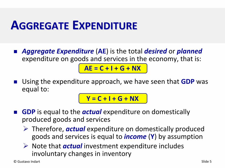
Aggregate Expenditure (AE) is the total desired or plannedexpenditure on goods and services in the economy, that is:

AE = C + I + G + NX

Using the expenditure approach, we have seen that GDP was equal to:

Y = C + I + G + NX

GDP is equal to the actual expenditure on domestically produced goods and services Therefore, actual expenditure on domestically produced

goods and services is equal to income (Y) by assumption Note that actual investment expenditure includes

involuntary changes in inventory© Gustavo Indart Slide 5

AGGREGATE EXPENDITURE


AGGREGATE EXPENDITURE (CONT’D)

The Aggregate Expenditure function indicates the desired level of expenditure at each level of income (Y) The Aggregate Expenditure function is an increasing

function of Y

Therefore, there must be a level of income at which desired aggregate expenditure (AE) is equal to actual aggregate expenditure (GDP = Y)

This level of income at which Y = AE is the equilibrium level of output or income (Y*) At Y* the goods market is in equilibrium The economy has produced (Y) exactly what economic

agents were planning to purchase (AE)


AGGREGATE EXPENDITURE (CONT’D)

If Y ≠ AE, then the economy is not in equilibrium If Y > AE excess supply in the goods market If Y < AE excess demand in the goods market

Since P is assumed fixed, then the implicit assumption is that aggregate expenditure determines the amount of goods produced in the economy

That is, Y must change in order to match AE and restore equilibrium in the economy Y must increase to eliminate an excess demand Y must decrease to eliminate an excess supply


A SIMPLE MODEL

Consider a simple model of an economy without government sector (G = 0) and without external sector (X = Q = 0)

Therefore, AE = C + I

How is equilibrium income (Y*) determined in this economy?


THE PLANNED (OR DESIRED) CONSUMPTION FUNCTION

The planned consumption function is a description of the total planned personal consumption expenditure by all households in the economy

Planned consumption expenditure depends on variables such as: Disposable income Wealth Interest rates Expectations about the future

Assumption: With the exception of disposable income, all the variables that determine planned consumption will be assumed constant

Assumption: Therefore, planned consumption will be assumed to be a function of disposable income (YD):

C = C + c YD

This equation indicates that planned consumption is equal to some constant (C) plus another constant (c) times disposable income (YD)


THE PLANNED CONSUMPTION FUNCTION


THE CONSUMPTION FUNCTION (CONT’D)

The constant C describes the elements of consumption which are independent of disposable income The constant C is called autonomous consumption and

captures the impact on C of all the constant variables

The constant c describes the rate of change of consumption as disposable income changes, that is, it indicates the increase in consumption per unit increase in disposable income:

∆Cc = ∆YD The constant c is called the marginal propensity to

consume out of disposable income (MPCYD)


MARGINAL PROPENSITY TO CONSUME

Since we are assuming that there is no government sector, taxes (TA) and transfer payments (TR) are nil Therefore, YD = Y This means that consumption is assumed to depend on

income (Y) alone:C = C + cY

Note that since Y = YD, then MPCY = MPCYD

However, as we will soon see, when YD differs from Y, MPCYalso differs from MPCYD

THE CONSUMPTION CURVE


C

YD

C

CSlope = c

C = C + cYD

●


14000

16000

18000

20000

22000

24000

26000

1981 1986 1991 1996 2001

2005

Dol

lars

Real Per Capita Disposable Income

Real Per Capita Expenditure

CANADA: PER CAPITA CONSUMPTIONAND DISPOSABLE INCOME (1981-2005)


MARGINAL PROPENSITY TO SAVE

The MPCYD is positive but less than 1, thus implying that a $1 increase in disposable income does not increase consumptionby $1

A fraction c is spent on consumption and the rest is saved (i.e., a fraction s = 1 − c is saved)

The constant s is the marginal propensity to save out of disposable income (MPSYD)

Therefore, c + s = 1


THE PLANNED SAVINGS FUNCTION

Since YD = C + S, the savings function is given by:S = YD − C

= YD − (C + cYD)= − C + (1 − c)YD= − C + sYD

Note that the MPSYD is also positive and less than 1 since s = 1 − c

The savings function is sort of the mirror image of the consumption function


CONSUMPTION AND SAVINGS FUNCTIONS

C, S

YD

C

S

C = C + c YDS = − C + (1 – c) YD

At the level of YD at which the C curve intersects the 45°line, C = YD and thus S = 0.

C

− C

When YD = 0, then C = C and S = – CC0 = YD0

For YD < YD0, C > YD and thus S < 0. For YD > YD0, C < YD and thus S > 0.

YD0

45°

•

•


THE PLANNED INVESTMENT FUNCTION

The investment function is a description of the total (desired or planned) investment expenditure by all private economic agents in the economy

In general, planned investment expenditure depends on: The real rate of interest The level of economic activity (Y) Businesses’ expectations about the behaviour of these

variables during the lifetime of the investment

I would argue that expectation about Y (and therefore about future demand) is the most relevant variable determining investment


THE PLANNED INVESTMENT FUNCTION

Assumption: For simplicity, we will assume that the rate of interest and expectations about the future are constant

Assumption: For simplicity, we will further assume that planned investment is independent of the level of income (Y)

Assumption: Therefore, planned investment will not change as the level of income (Y) changes

I is equal to autonomous investment: I = I

THE INVESTMENT CURVE


I

Y

II

I = I

●


THE AGGREGATE EXPENDITURE FUNCTION

In this very simple model, the aggregate expenditurefunction is:

AE = C + I= (C + cY) + I= (C + I) + cY= AE + cY

where AE = C + I is autonomous aggregate expenditure and cYis induced aggregate expenditure

AE is the vertical intercept of the AE function, and c is the slope of the AE function (or the marginal propensity to spend)

AGGREGATE EXPENDITURE FUNCTION


AECI

Y

C

C = C + cYI = IAE = AE + cY

C

Slope = cI

AE

AE = C + I

I

I

●

●

●

We have seen that in equilibrium, output (GDP) or income (Y) is equal to aggregate expenditure (AE):

Y = AE= AE + cY

Therefore, Y – cY = AE(1 – c)Y = AE

and equilibrium income is:1

Y* = AE1 – c

EQUILIBRIUM INCOME AND OUTPUT


AGGREGATE EXPENDITURE FUNCTION


Y

AE = AE + cY

Slope = cAE

AEGDP

AE

45°Y*

At Y = Y*, Y = AE and thus actual investment is equal to desired investment There is no involuntary change in inventories.

At Y = Y1, Y > AE and thus actual investment is greater than desired investment There is an involuntary increase in inventories.

At Y = Y2, Y < AE and thus actual investment is smaller than desired investment There is an involuntary decrease in inventories.Y1Y2

Actual Expenditure

CONSUMPTION AND SAVING

The implicit assumption is that actual consumption is always equal to desired consumption as a result of involuntarychanges in inventory

If AE > Y, there is an involuntary decrease in inventory to satisfy the level of desired consumption

If AE < Y, there is an involuntary increase in inventory because desired consumption is not enough (i.e., saving is too large)

Therefore, since actual consumption and desiredconsumption are always equal, then actual saving and desired saving are always equal as well


By definition, savings is equal to actual investment Output (GDP) is equal to income (Y) by assumption Income not spend on consumption is saved Output not used for consumption is used for investment

Y = C + S and Y = C + actual I S = actual I In equilibrium, when Y = AE, there is no involuntary change in

inventory Therefore, desired and actual investment are equal

Therefore, in a closed economy with no government sector, If Y = AE, then S = desired I If Y < AE, then S < desired I If Y > AE, then S > desired I

SAVINGS AND INVESTMENT


TWO WAYS OF EXPRESSING EQUILIBRIUMINCOME IN THE ECONOMY


AEGDP

SY

Y

AE

S

S = − C + (1 – c)YI = IAE = AE + cY

Y = AE at Y = Y*, and thus Y* is the equilibrium level of income.

Y*

45°

I

− C

AE

Y*

I S = I at Y = Y*, and thus Y* is the equilibrium level of income.

Actual Expenditure

SAVINGS AND INVESTMENT

By definition, savings is always equal to actual investment Question: If high rates of investment are desirable, are high

rates of savings also desirable? If savings determine productive investment, then high

rates of savings might be desirable But high desired savings is the result of low desired

consumption expenditure Therefore, actual investment is large because firms are

experiencing involuntary increases in inventory Therefore, higher desired savings does not translate into

higher productive capacity of the economy But higher desired investment does translate into higher Y

and thus into higher desired savings© Gustavo Indart Slide 28

SAVINGS AND INVESTMENT (CONT’D)


AEGDP

SY

Y

AE

S

S = − C + (1 – c)YI = IAE = AE + cY

Initially the economy is in equilibrium at Y1.Y1

45°

I

− C1

AE1

Y1

I

As desired savings increases to S’ and aggregate expenditure decreases to AE’, Y > AE and Y falls.

AE’

AE2

Y2

Y2− C2

S’

•

•

How does a change in autonomous expenditure (AE) affect equilibrium income (Y*)?

The equation for equilibrium income shows that a ∆AE will affect Y* in the following way:

1∆Y* = ∆AE

1 – c The expression

∆Y* 1 1αAE = = =

∆AE 1 – c 1 – slope of AE curveis called the autonomous expenditure multiplier or just the multiplier

THE MULTIPLIER


1Y* = AE

1 – c

THE MULTIPLIER (CONT’D)

A change in autonomous expenditure (ΔAE) causes equilibrium income (Y*) to change by the initial change in AEtimes the multiplier (αAE)

This change in Y*, αAE ΔAE, is the final result and does not show the process leading to it

Let’s have a look at the process leading to this final outcome

Suppose that autonomous expenditure increases by ∆AE


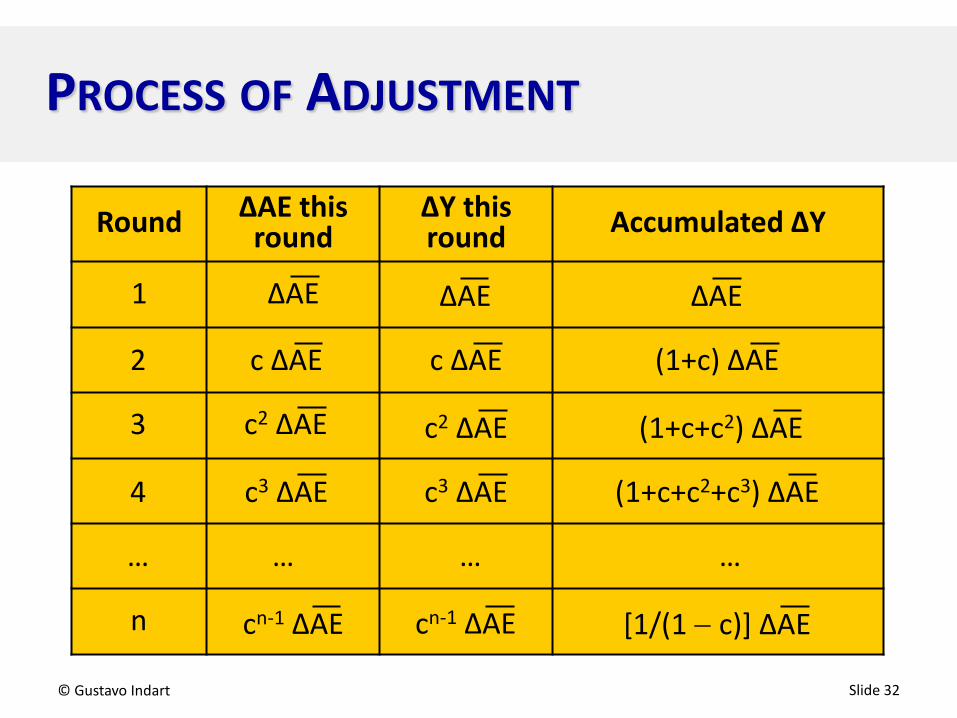
PROCESS OF ADJUSTMENT


Round ∆AE this round

∆Y this round Accumulated ∆Y

1 ∆AE ∆AE ∆AE

2

3

4

c ∆AE c ∆AE (1+c) ∆AE

c2 ∆AE c2 ∆AE (1+c+c2) ∆AE

… … … …

n [1/(1 − c)] ∆AE

c3 ∆AE c3 ∆AE (1+c+c2+c3) ∆AE

cn-1 ∆AE cn-1 ∆AE

After n rounds, the series 1 + c + c2 + c3+… converges to αAE = 1/(1 – c)

Let’s call a = 1 + c + c2 + c3 + …

Multiply a by c ca = c + c2 + c3 + …

Now subtract ca from a: a – ca = (1 + c + c2 + c3 +…) – (c + c2 + c3 +…) = 1

Therefore, a (1 – c) = 1 a = 1/(1 – c)

PROCESS OF ADJUSTMENT (CONT’D)


INTRODUCTION OF THE GOVERNMENTSECTOR

Disposable income (YD) changes: Households pay taxes Households receive transfer payments

Equation for AE changes: AE = C + I + G

We will assume that government expenditure on goods and services is independent of the level of income, that is, G is fixed G = G



DISPOSABLE INCOME AND THECONSUMPTION FUNCTION

We have seen that consumption is a function of disposable income (YD):

C = C + cYDwhere C is autonomous consumption and c is the marginal propensity to consume out of disposable income (MPCYD)

Disposable income (YD) is equal to:YD = Y + TR – TA

where TR are government transfer payments and TA are direct taxes

DISPOSABLE INCOME AND THECONSUMPTION FUNCTION (CONT’D)

Let’s assume that taxes are a function of income and that transfer payments are independent of income: TA = T + tY TR = TR

Therefore, disposable income is equal to:YD = Y + TR – (T + tY)

= TR – T + (1 – t)Y


THE CONSUMPTION FUNCTION AS AFUNCTION OF INCOME

As a function of income, the consumption function is:C = C + cYD

= C + c [ TR – T + (1 – t)Y ] = (C + cTR – cT) + c(1 – t)Y

That is, (C + cTR – cT) is the vertical intercept and c(1 – t) is the slope

Note that c(1 – t) is the marginal propensity to consume out of income (MPCY)

Also note that MPCY < MPCYD if t > 0


YD = TR − T + (1 − t)Y

THE AGGREGATE EXPENDITURE FUNCTION

The aggregate expenditure function is:AE = C + I + G

= [ C + cTR – cT + c(1 – t)Y ] + I + G= AE + c(1 – t)Y

where AE = C + cTR – cT + I + G

The vertical intercept is AE and the slope is c(1 – t)

Recall that the slope of the AE curve is the marginal propensity to spend


Equilibrium income is determined where Y = AE:Y = AE + c (1 – t)Y[ 1 – c (1 – t) ] Y = AE

Therefore,1

Y* = AE1 – c (1 – t)

EQUILIBRIUM OUTPUT AND INCOME


The autonomous expenditure multiplier becomes:1

αAE = 1 – c(1 – t)

Note that as before, the multiplier is equal to 1 over 1 minus the slope of the AE curve

Also note that, as t increases, αAE becomes smaller (the AEcurve becomes flatter)

What’s the economic explanation?© Gustavo Indart Slide 40

THE MULTIPLIER

THE INTRODUCTION OF THEFOREIGN SECTOR

We will assume that the equations for exports (X) and imports (Q) are as follows:

X = XQ = Q + mY

where m is the marginal propensity to import

Therefore, the equation for net exports (NX) is:NX = X – Q

= X – Q – mY


THE EQUATION FOR THE AE CURVE

In a closed economy, the equation for AE was:AE = C + I + G

= AE + c(1 – t)Ywhere AE = C – cT + cTR + I + G

In an open economy, the equation for AE is:AE = C + I + G + NX

= AE + [c(1 – t) – m]Ywhere AE = C – cT + cTR + I + G + X – Q


NX = X – Q − mY

In equilibrium, Y = AE, that is,Y = AE + [c(1 – t) – m]Y

{1 – [c(1 – t) – m]}Y = AE

Therefore, equilibrium income is:

1Y* = AE

1 – c(1 – t) + m

where AE = C – cT + cTR + I + G + X – Q

EQUILIBRIUM INCOME


THE MULTIPLIER

The multiplier is:1

αAE =1 – c(1 – t) + m

1=

1 – slope of the AE curve

Where the slope of the AE curve (i.e., the marginal propensity to spend) is the fraction of each additional dollar of income which is spent on domestically produced goods


eco 209y macroeconomic theory and policy 03 - eco 209... · assumptions we will assume that: there...

Documents