eco-drive experiment on rolling terrain for fuel consumption optimization … · 2018-03-28 ·...
TRANSCRIPT

ECO-DRIVE EXPERIMENT ON ROLLING TERRAIN FOR FUEL CONSUMPTION OPTIMIZATION SUMMARY REPORT Publication No. FHWA-HRT-18-037
HRDO-20/04-18(WEB)E
March 2018
Turner-Fairbank Highway Research Center6300 Georgetown PikeMcLean, VA 22101-2296

FOREWORD The Turner-Fairbank Highway Research Center (TFHRC) performs advanced research into several areas of transportation technology for the Federal Highway Administration (FHWA). The Office of Operations Research and Development (HRDO) focuses on improving operations-related technology through research, development, and testing. This report summarizes a research project sponsored by HRDO to evaluate the ability of a longitudinal control algorithm to improve the fuel economy of a vehicle on rolling terrain. These promising results provide an excellent justification for the implementation of vehicle-to-infrastructure (V2I) technology that would appeal to roadway owners, roadway users, and original equipment manufacturers (OEMs).
Brian Cronin, Director, Office of Operations Research and Development
Notice
This document is disseminated under the sponsorship of the U.S. Department of Transportation (USDOT) in the interest of information exchange. The U.S. Government assumes no liability for the use of the information contained in this document. The U.S. Government does not endorse products or manufacturers. Trademarks or manufacturers’ names appear in this report only because they are considered essential to the objective of the document.
Quality Assurance Statement
The Federal Highway Administration (FHWA) provides high-quality information to serve Government, industry, and the public in a manner that promotes public understanding. Standards and policies are used to ensure and maximize the quality, objectivity, utility, and integrity of its information. FHWA periodically reviews quality issues and adjusts its programs and processes to ensure continuous quality improvement.

TECHNICAL REPORT DOCUMENTATION PAGE 1. Report No. FHWA-HRT-18-037
2. Government Accession No. 3 Recipient's Catalog No.
4. Title and Subtitle Eco-Drive Experiment on Rolling Terrain for Fuel Consumption Optimization – Summary Report
5. Report Date September 26, 2017
6. Performing Organization Code
7. Author(s) Jiaqi Ma, Ph.D.; Jia Hu, Ph.D.; Ed Leslie; Fang Zhou; Zhitong Huang, Ph.D.
8. Performing Organization Report No.
9. Performing Organization Name and Address Leidos Inc. 11251 Freedom Dr. Reston, VA
10. Work Unit No. (TRAIS)
11. Contract or Grant No. DTFH6116D00030 Task Order 07
12. Sponsoring Agency Name and Address Office of Highway Operations Research and Development Federal Highway Administration 6300 Georgetown Pike McLean, VA 22101-2296
13. Type of Report and Period Covered
14. Sponsoring Agency Code Code HRDO-20
15. Supplementary Notes Peter Huang, Ph.D.; Joe Bared, Ph.D. – FHWA Task Managers
16. Abstract Eco-drive is one of the many theoretical concepts that have been developed to increase vehicle fuel efficiency and improve the sustainability of the entire transportation system within the connected vehicle paradigm. This study proposes an eco-drive algorithm for vehicle fuel consumption optimization on rolling terrains, which frequently cause additional fuel waste because of inefficient transformation between kinetic and potential energy. The algorithm uses the Relaxed Pontryagin’s Minimum Principle (RPMP), is computationally efficient, and is applicable in real time. While similar algorithms have proven effective in simulation with many assumptions, it is necessary to test these algorithms in the field to better understand the algorithm’s performance and thus enable optimal vehicle control in support of eco-driving. Therefore, this study further tested and verified the newly developed algorithms on an innovative connected and automated vehicle (CAV) platform and quantified the fuel saving benefits of eco-drive. The proposed eco-drive system is compared against conventional constant-speed cruise control on a total of 7 road segments over 47 miles. Experimental data show that more than 20 percent of fuel consumption can be avoided on certain terrains. Detailed analysis through linear models also reveals the main geometrical contributors to eco-drive fuel savings. This conclusion can enable a rough estimate of fuel saving potential on given roadways and help State departments of transportation to identify roadways where eco-drive should be implemented. The algorithm and the experiment can also support original equipment manufacturers in developing and marketing this technology to reduce fuel consumption and emissions in the future.
17. Key Words Eco-Drive, Fuel Economy, Connected Automated Vehicle, Fuel Optimization
18. Distribution Statement No restrictions. This document is available to the public through the National Technical Information Service, Springfield, VA 22161. http://www.ntis.gov
19. Security Classification (of this report) Unclassified
20. Security Classification (of this page) Unclassified
21. No. of Pages 49
22. Price
Form DOT F 1700.7 (8-72) Reproduction of completed page authorized

ii

iii
TABLE OF CONTENTS
EXECUTIVE SUMMARY ........................................................................................................... 1
CHAPTER 1. INTRODUCTION ................................................................................................ 3
CHAPTER 2. RESEARCH OBJECTIVE .................................................................................. 7
CHAPTER 3. VEHICLE CONTROL FORMULATION AND DESIGN ............................... 9
UPPER-LEVEL CONTROLLER – TRAJECTORY PLANNING FOR OPTIMAL SPEED PROFILES ...................................................................................................................................... 9
State Explanation ................................................................................................................ 9 Cost Function ...................................................................................................................... 9 Vehicle Dynamic Model ....................................................................................................11 Constraints and Initial Conditions .....................................................................................11 Solution Based on Pontryagin’s Minimum Principle (PMP) ............................................ 12 Iterative PMP Solving Process .......................................................................................... 13
SECONDARY SPEED CONTROLLER ...................................................................................... 14 Brake Reduction................................................................................................................ 14 Speed Limit ....................................................................................................................... 14 PID Control ....................................................................................................................... 15
CHAPTER 4. EXPERIMENTAL VEHICLE PLATFORM ................................................... 17
CHAPTER 5. FIELD EXPERIMENT AND RESULTS ......................................................... 21
EXPERIMENT DESIGN .............................................................................................................. 21 ROADWAY PROFILE DATA VALIDATION ............................................................................. 22 ANALYSIS METHODOLOGY AND RESULTS ........................................................................ 22
Segment Data Analysis ..................................................................................................... 22 Subsegment Data Analysis ................................................................................................ 27
CHAPTER 6. CONCLUSIONS AND FUTURE RESEARCH............................................... 31
APPENDIX .................................................................................................................................. 33
ACKNOWLEDGMENTS .......................................................................................................... 37
REFERENCES ............................................................................................................................ 39

iv
LIST OF FIGURES Figure 1. Concept of V2I-based eco-drive on rolling terrains. ....................................................... 4 Figure 2. Vehicle secondary speed controller diagram. ................................................................ 14 Figure 3. Data flow of the vehicle control systems (Ma, Leslie, and Zhou, 2018). ..................... 18 Figure 4. Installation of the fuel flowmeter. ................................................................................. 19 Figure 5. CAV vehicle fleet. .......................................................................................................... 19 Figure 6. Vehicle control devices. ................................................................................................. 20 Figure 7. Fuel meter installed at vehicle fuel line. ........................................................................ 20 Figure 8. Speed Profile results at the segmental level for example runs (Source: FHWA). ......... 23 Figure 9. Experimental results at segmental level for example runs (Source: FHWA). ............... 25 Figure 10. Illustration of subsegments of River Road NB profile. ............................................... 27 Figure 11. Road data for Georgetown Pike from Colonial Farm Road to I–495. ......................... 33 Figure 12. Road data for George Washington Parkway Northbound from Key Bridge to I–495. 34 Figure 13. Road data for George Washington Parkway Southbound from I–495 to Key Bridge. 34 Figure 14. Road data for River Road from Seven Locks Road to Seneca Road. ......................... 35 Figure 15. Road data for River Road from Seneca Road to Seven Locks Road. ......................... 35 Figure 16. Road data for US–17 from US–17 Business to I–66. .................................................. 36 Figure 17. Road data for US–17 from I–66 to US–17 Business. .................................................. 36
LIST OF TABLES
Table 1. Segment level Results of eco-drive benefits. .................................................................. 26 Table 2. Subsegment level Results of eco-drive benefits. ............................................................ 29

1
EXECUTIVE SUMMARY Eco-drive is one of the many research topics that address the issue of increasing vehicle fuel efficiency and improving the sustainability of the entire transportation system. Connected and automated vehicle (CAV) data are now being used to allow vehicles to cooperate better with current and future environments, including traffic conditions, signal timing, and terrain information. This study proposes an eco-drive algorithm for vehicle fuel consumption optimization on rolling terrains, which frequently cause additional fuel waste because of inefficient transformation between kinetic and potential energy. The proposed algorithm uses the Relaxed Pontryagin’s Minimum Principle (RPMP); it is computationally efficient and applicable in real time. While similar algorithms have proven effective in simulation with many assumptions, it is necessary to test these algorithms in the field to better understand the algorithm’s performance and thus enable optimal vehicle control in support of eco-driving. Therefore, this study further tested and verified the newly developed algorithms on an innovative CAV platform and quantified the fuel saving benefits of eco-drive. The proposed eco-drive system is compared against conventional constant-speed cruise control on a total of seven road segments over 47 miles. Experimental data show that more than 20 percent of fuel consumption can be avoided on certain terrains. Detailed analysis through linear models also reveals the main geometrical contributors to the eco-drive fuel savings. This conclusion can enable a rough estimate of fuel saving potential on given roadways and help State departments of transportation to identify roadways where eco-drive could be beneficial. The algorithm and the experiment can also support original equipment manufacturers in developing and marketing this technology to reduce fuel consumption and emissions in the future. Further research is still needed to study the impact of this univariate finding on following traffic, including automated and nonautomated vehicles.


3
CHAPTER 1. INTRODUCTION Accomplishments in individual vehicle control have laid the foundation for more advanced control that governs interactions among multiple connected vehicles (CVs) and can produce resultant effects on highway traffic performance. Efforts have been made to extend adaptive cruise control (ACC) to cooperative adaptive cruise control (CACC) to further improve vehicle-following efficiency through multivehicle communication that takes stability (Vugts, 2010), traffic throughput (Van Arem, 2005), and energy and environmental impacts (Malakorn & Park, 2010; Ma et al., 2016) into account. Limited attempts have been made to extend these developments to other, more complex infrastructure geometries, such as ramp merges (Park & Smith, 2012) and intersections (Drenser & Stone, 2012; Zhou et al., 2016; Hu et al., 2015). However, most of these studies apply simulation to evaluate the effectiveness and benefits of control algorithms. Field experiments must now be undertaken to show that new technologies function as expected in practice and to collect data on control system performance under nontheoretical conditions (e.g., mixed traffic, system delay, or inaccurate input data) as basis for further system improvement. Eco-drive is one of the many research topics that address the issue of vehicle fuel efficiency. CV data are now being leveraged to allow vehicles to cooperate better within the current and future environments in terms of traffic conditions, signal timing, and terrain information. This study investigates the use of vehicle automation and mobile communication technology to derive the maximum benefits from eco-drive. The concept of vehicle-to-infrastructure (V2I)-based eco-drive is illustrated in figure 1. Traffic management centers (TMCs) maintain databases of all roadway profiles (i.e., location, horizontal and vertical curves, work zones, etc.). In this concept, TMCs predefine a list of roadway segments on which automated eco-drive is recommended or enforced. These segments are selected because of their potential for significant fuel savings according to segment characteristics. Once the eco-drive vehicle receives information from the TMC, an onboard computer equipped with a preloaded algorithm will design a recommended trajectory (i.e., speed profile) for the vehicle to traverse the entire rolling segment. This algorithm should also account for other factors such as vehicle operating capability, driver comfort, safety, and speed limits. Advanced algorithms may also account for the existence of a front vehicle (via vehicle-to-vehicle (V2V) communication) and downstream traffic congestion through the addition of speed harmonization (Ma et al., 2016) components to the algorithm. But these advancements are out of the scope of this study and will be left for future exploration. In this paper, the term “eco-drive” is used to refer to this specific concept of V2I-based eco-drive on rolling terrains. Note that this roadway profile information is usually collected through roadway survey and design documents from State department of transportation (DOT) construction divisions, which are generally only available for newly constructed, major roads. In the future, with increasingly accurate and prevailing vehicular onboard sensors, CVs (eco-drive or not) can potentially send real-time information related to roadway geometry (e.g., latitude, longitude, altitude) to TMCs to update roadway profile databases, particularly in cases where changes in geometry occur, or to collect information on roadways where no profile data are available. This study also explores advanced Global Position System (GPS) service to extract roadway profile data.

4
Source: FHWA
Figure 1. Concept of V2I-based eco-drive on rolling terrains.
Given that roadway geometry data collected via connected vehicle technologies are much more accessible than those from design/survey documents, researchers believe that CV geometry data are more likely than survey data to be used as input for potential eco-drive applications. Therefore, this experiment purposefully used CV geometry data as input. It is one of the many very important designs this experiment adopts to ensure the eco-drive application is tested under the most realistic environment. Past research validated that a 6 percent increase in roadway grade resulted in a 40 to 94 percent increase in fuel consumption (Park & Rakha, 2006). Another study confirmed that fuel economy on flat routes is superior to that on rolling or mountainous routes by approximately 15 to 20 percent (Boriboonsomsin & Barth, 2009). However, in theory, if no energy is wasted, vehicles driving on rolling terrain should consume the same amount of fuel as vehicles driving on flat roads. The only difference between the two is the fact that the vehicles on rolling terrain constantly have energy transferring between potential energy and kinetic energy. Therefore, these studies concluded, the increase in fuel consumption resulted in additional unnecessary waste, which can be avoided or reduced by optimizing vehicle states. Some studies have investigated vehicle speed and powertrain optimization (Hellström, et al., 2010), but these approaches are over simplified or are not yet ready for real world implementation. For example, these particular approaches only consider constant slope scenarios. Further, the algorithms used—such as dynamic programming—are computationally intensive and difficult to apply in real time. A recent study shows that using CV technology on a hybrid electric vehicle (with speed and powertrain optimization algorithms) could gain up to 17 percent fuel savings on rolling terrain (Hu et al., 2016). Further research for regular gasoline engines shows the benefit of the proposed optimal controller is significant compared to cruising on rolling terrain at a constant speed, with fuel saving ranging from 11.7 to 16.3 percent (Hu et al., 2016). Both studies show great potential in significantly reducing fuel consumption for a stretch of roadway with changing terrain, and

5
the proposed algorithms using the Relaxed Pontryagin’s Minimum Principle (RPMP) are computationally efficient and applicable in real time. While these new algorithms prove effective in simulation with many assumptions, it is necessary to test these algorithms in real-world scenarios to better understand the algorithm performance, and thus improve them to optimally control vehicles for eco-drive. Following this introduction, this report provides a brief review of the innovative vehicle control platform, including algorithm design and system logic. Then the experimental design for the field experiment and testing environment is described, followed by a discussion of the experiment. The last section discusses conclusions and future research.


7
CHAPTER 2. RESEARCH OBJECTIVE The objective of this study is to propose an efficient algorithm and test it on a vehicle platform such that the potential benefit of eco-drive can be quantified in a real-world environment. The experiment was conducted on various vertical alignments using a Federal Highway Administration (FHWA) Saxton Transportation Operations Laboratory (STOL) research vehicle (2013 Cadillac SRX with a regular gasoline engine) and by controlling the speed only as estimated by the given algorithm. It is hoped that the algorithm and the experiment will support State DOTs and original equipment manufacturers (OEMs) in developing and marketing this technology to reduce fuel consumption and emissions. The contributions made by this research include:
1. Developing and enhancing the eco-drive algorithm (Hu et al., 2016) using the RPMP that is computationally efficient and applicable in real time.
2. Executing field experiments with an innovative vehicle control platform that includes recent vehicular and communication technologies.
3. Quantifying eco-drive benefits in a real-world environment and providing decisionmakers with data and tools for better management strategies.


9
CHAPTER 3. VEHICLE CONTROL FORMULATION AND DESIGN This section introduces the two speed controllers used in our experiment. The first is an upper-level controller that is responsible for trajectory planning to generate optimal speed profiles. The other is a secondary controller that adjusts speed commands in real time for enhanced performance and contains a classic proportional-integral-derivative (PID) controller for vehicle speed following. The recommended speed profiles generated from the upper-level controller will be filtered by the secondary controller and sent to the vehicle for execution. UPPER-LEVEL CONTROLLER – TRAJECTORY PLANNING FOR OPTIMAL SPEED PROFILES This section describes the formulation of the vehicle upper-level controller. The controller optimizes vehicle fuel efficiency, mobility, and comfort. The inputs for this controller are the vehicle’s current speed and location together with the future road’s altitude and dynamic speed limit. The output of this controller is an optimal acceleration/speed trajectory. State Explanation In this experiment, a system of one single vehicle is considered. The system’s state vector 𝒙𝒙 is defined as a vector consisting of the distance from the trip origin and the vehicle’s instant speed, as seen in equation 1.
(1)
Where: 𝑥𝑥1(𝑡𝑡) = the distance from the origin (m). 𝑥𝑥2(𝑡𝑡) = the vehicle’s instant speed (m/s).
The state dynamics are defined in equation 2.
(2)
Where
𝑢𝑢1(𝑡𝑡) = the controlled acceleration for the test vehicle. Cost Function The cost function J is defined in equation 3.
(3)
𝒙𝒙(𝑡𝑡) = [𝑥𝑥1(𝑡𝑡) 𝑥𝑥2(𝑡𝑡)]𝑇𝑇
�̇�𝒙(𝑡𝑡) = 𝑓𝑓(𝒙𝒙,𝑢𝑢1) = [𝑥𝑥2(𝑡𝑡) 𝑢𝑢1(𝑡𝑡)]𝑇𝑇
𝐽𝐽 = 𝜓𝜓(𝒙𝒙(𝑇𝑇)) + � 𝐿𝐿(𝒙𝒙,𝑢𝑢1)𝑡𝑡0+𝑇𝑇
𝑡𝑡0
𝑑𝑑𝑡𝑡
10
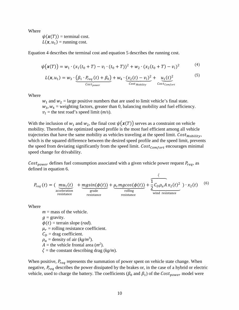
Where 𝜓𝜓(𝒙𝒙(𝑇𝑇)) = terminal cost. 𝐿𝐿(𝒙𝒙,𝑢𝑢1) = running cost.
Equation 4 describes the terminal cost and equation 5 describes the running cost.
(4)
(5)
Where
𝑤𝑤1 and 𝑤𝑤2 = large positive numbers that are used to limit vehicle’s final state. 𝑤𝑤3,𝑤𝑤4 = weighting factors, greater than 0, balancing mobility and fuel efficiency. 𝑣𝑣𝑙𝑙 = the test road’s speed limit (m/s).
With the inclusion of 𝑤𝑤1 and 𝑤𝑤2, the final cost 𝜓𝜓�𝒙𝒙(𝑇𝑇)� serves as a constraint on vehicle mobility. Therefore, the optimized speed profile is the most fuel efficient among all vehicle trajectories that have the same mobility as vehicles traveling at the speed limit. 𝐶𝐶𝐶𝐶𝐶𝐶𝑡𝑡𝑀𝑀𝑀𝑀𝑀𝑀𝑀𝑀𝑙𝑙𝑀𝑀𝑀𝑀𝑀𝑀, which is the squared difference between the desired speed profile and the speed limit, prevents the speed from deviating significantly from the speed limit. 𝐶𝐶𝐶𝐶𝐶𝐶𝑡𝑡𝐶𝐶𝑀𝑀𝐶𝐶𝐶𝐶𝑀𝑀𝐶𝐶𝑀𝑀 encourages minimal speed change for drivability. 𝐶𝐶𝐶𝐶𝐶𝐶𝑡𝑡𝑝𝑝𝑀𝑀𝑝𝑝𝑝𝑝𝐶𝐶 defines fuel consumption associated with a given vehicle power request 𝑃𝑃𝐶𝐶𝑝𝑝𝑟𝑟, as defined in equation 6.
(6)
Where
m = mass of the vehicle. 𝑔𝑔 = gravity. 𝜙𝜙(𝑡𝑡) = terrain slope (rad). 𝜇𝜇𝐶𝐶 = rolling resistance coefficient. 𝐶𝐶𝐷𝐷 = drag coefficient. 𝜌𝜌𝑎𝑎 = density of air (kg/m3). 𝐴𝐴 = the vehicle frontal area (m2). 𝜁𝜁 = the constant describing drag (kg/m).
When positive, 𝑃𝑃𝐶𝐶𝑝𝑝𝑟𝑟 represents the summation of power spent on vehicle state change. When negative, 𝑃𝑃𝐶𝐶𝑝𝑝𝑟𝑟 describes the power dissipated by the brakes or, in the case of a hybrid or electric vehicle, used to charge the battery. The coefficients (𝛽𝛽0 and 𝛽𝛽1) of the 𝐶𝐶𝐶𝐶𝐶𝐶𝑡𝑡𝑝𝑝𝑀𝑀𝑝𝑝𝑝𝑝𝐶𝐶 model were
𝜓𝜓�𝒙𝒙(𝑇𝑇)� = 𝑤𝑤1 ∙ (𝑥𝑥1(𝑡𝑡0 + 𝑇𝑇) − 𝑣𝑣𝑙𝑙 ∙ (𝑡𝑡0 + 𝑇𝑇))2 + 𝑤𝑤2 ∙ (𝑥𝑥2(𝑡𝑡0 + 𝑇𝑇) − 𝑣𝑣𝑙𝑙)2
𝐿𝐿(𝒙𝒙,𝑢𝑢1) = 𝑤𝑤3 ∙ �𝛽𝛽1 ∙ 𝑃𝑃𝑟𝑟𝑟𝑟𝑟𝑟 (𝑡𝑡) + 𝛽𝛽0��������������𝐶𝐶𝐶𝐶𝐶𝐶𝑡𝑡𝑝𝑝𝐶𝐶𝑤𝑤𝑟𝑟𝑟𝑟
+ 𝑤𝑤4 ∙ (𝑥𝑥2(𝑡𝑡) − 𝑣𝑣𝑙𝑙)2���������𝐶𝐶𝐶𝐶𝐶𝐶𝑡𝑡𝑀𝑀𝐶𝐶𝑀𝑀𝑀𝑀𝑙𝑙𝑀𝑀𝑡𝑡𝑀𝑀
+ 𝑢𝑢1(𝑡𝑡)2���𝐶𝐶𝐶𝐶𝐶𝐶𝑡𝑡𝐶𝐶𝐶𝐶𝐶𝐶𝑓𝑓𝐶𝐶𝑟𝑟𝑡𝑡
𝑃𝑃𝑟𝑟𝑟𝑟𝑟𝑟 (𝑡𝑡) = ( 𝐶𝐶𝑢𝑢1(𝑡𝑡)�����acceleration
resistance
+ 𝐶𝐶𝑔𝑔𝐶𝐶𝑀𝑀𝑚𝑚(𝜙𝜙(𝑡𝑡))���������grade
resistance
+ 𝜇𝜇𝑟𝑟𝐶𝐶𝑔𝑔𝑚𝑚𝐶𝐶𝐶𝐶(𝜙𝜙(𝑡𝑡))����������� rolling
resistance
+12𝐶𝐶𝐷𝐷𝜌𝜌𝑎𝑎𝐴𝐴
�����𝜁𝜁
𝑥𝑥2(𝑡𝑡)2�����������
wind resistance
) ∙ 𝑥𝑥2(𝑡𝑡)

11
acquired by fitting a linear equation representing power request against fuel consumption (Hu et al., 2016). Vehicle Dynamic Model The longitudinal vehicle dynamics model is shown in equation 7.
(7)
Where
𝐹𝐹𝑀𝑀 is the thrust force. Constraints and Initial Conditions Acceleration constraint: To ensure the feasibility of acceleration commands given the brake condition and engine maximum power constraints, the maximum acceleration is set as (Fmax- FR)/m m/s2, and maximum deceleration is set as -5 m/s2. Fmax is the maximum thrust force of the powertrain and FR is the summation of the three resistant forces (see equation 7). Note that this acceleration constraint is solely for the eco-drive controller. When a safety hazard arises, collision prevention applications can overrule this constraint and provide much greater deceleration. This constraint can be expressed as a permissible set of acceleration, shown in equation 8.
(8)
Speed constraint: Due to safety considerations, the speed change range is predetermined. In this study, maximum speed is 4.48 m/s (10 mph) above the speed limit and minimum speed is 4.48 m/s (10 mph) below the speed limit. This constraint is specified in equation 9.
(9)
Vehicle dynamic constraints: The dynamics of the vehicle should follow the laws of physics, specifically those defined in equation 2. The initial conditions are shown in equations 10 and 11.
(10)
(11)
𝐶𝐶𝑢𝑢1(𝑡𝑡)���vehicle
acceleration
= 𝐹𝐹𝑡𝑡 − (𝐶𝐶𝑔𝑔𝐶𝐶𝑀𝑀𝑚𝑚�𝜙𝜙(𝑡𝑡)����������grade
resistance
+ 𝜇𝜇𝑟𝑟𝐶𝐶𝑔𝑔𝑚𝑚𝐶𝐶𝐶𝐶�𝜙𝜙(𝑡𝑡)������������ rolling
resistance
+12𝐶𝐶𝐷𝐷𝜌𝜌𝑎𝑎𝐴𝐴𝑥𝑥2(𝑡𝑡)2
���������wind resistance
)
𝒰𝒰𝑣𝑣 = {𝑢𝑢1|𝑢𝑢min ≤ 𝑢𝑢1(𝑡𝑡) ≤ 𝑢𝑢max ,∀𝑡𝑡 ∈ [𝑡𝑡0, 𝑡𝑡0 + 𝑇𝑇]}
𝒱𝒱𝑣𝑣 = {𝑥𝑥2|𝑣𝑣min ≤ 𝑥𝑥2(𝑡𝑡) ≤ 𝑣𝑣max ,∀𝑡𝑡 ∈ [𝑡𝑡0, 𝑡𝑡0 + 𝑇𝑇]}
𝑥𝑥1(𝑡𝑡0) = 𝑥𝑥0
𝑥𝑥2(𝑡𝑡0) = 𝑣𝑣0

12
Solution Based on Pontryagin’s Minimum Principle (PMP) In general, PMP entails defining the Hamiltonian ℋ as shown in equation 12.
(12)
Where
𝝀𝝀 = the gradient of the total cost-to-go of the state 𝒙𝒙.
In other words, 𝜆𝜆 is the extra cost of 𝐽𝐽 caused by a small change ∂𝒙𝒙 on the state 𝒙𝒙. 𝝀𝝀 is also known as the co-state. According to PMP, for all control values that fall within the parameters of permissible controls set 𝒰𝒰, the optimal control 𝒖𝒖∗ must satisfy the requirements in equation 13.
(13)
The above Hamiltonian law could be expressed alternatively as the necessary conditions in equation 14.
(14)
Equation 14(iii) is equivalent to the vehicle dynamics. Equations 14(i) and 14(ii) serve to solve for optimal control. For vehicle-level optimization, substitute Hamiltonian ℋ with the cost function of this study, shown in equation 15.
(15)
Applying the condition in equation 14(i) to the cost function gives equation 16.
(16)
Equation 16 can be rearranged to provide the control law in equation 17.
(17)
Applying the condition in equation 14(ii) to the cost function gives equations 18 and 19.
ℋ(𝒙𝒙,𝒖𝒖,𝝀𝝀, 𝑡𝑡) = 𝝀𝝀𝑇𝑇 ∙ 𝑓𝑓(𝒙𝒙,𝒖𝒖, 𝑡𝑡) + 𝐿𝐿(𝒙𝒙,𝒖𝒖, 𝑡𝑡)
ℋ(𝒙𝒙∗,𝒖𝒖∗,𝝀𝝀∗, 𝑡𝑡) ≤ ℋ(𝒙𝒙∗,𝒖𝒖,𝝀𝝀∗, 𝑡𝑡), ∀𝒖𝒖 ∈ 𝒰𝒰, 𝑡𝑡 ∈ [𝑡𝑡0, 𝑡𝑡0 + 𝑇𝑇]
(i) 0 = ∂ℋ∂𝒖𝒖
, (ii) �̇�𝝀 = −𝜕𝜕ℋ𝜕𝜕𝒙𝒙
, (iii) �̇�𝒙 = 𝜕𝜕ℋ𝜕𝜕𝝀𝝀
𝜕𝜕ℋ𝜕𝜕𝑢𝑢
(𝒙𝒙,𝑢𝑢1,𝝀𝝀) = 𝜆𝜆2(𝑡𝑡) + 𝑤𝑤3 ∙ [𝐶𝐶 ∙ 𝛽𝛽1 ∙ 𝑥𝑥2(𝑡𝑡)] + 2 ∙ 𝑢𝑢1(𝑡𝑡) = 0
𝑢𝑢1(𝑡𝑡) =𝜆𝜆2(𝑡𝑡) + 𝑤𝑤3 ∙ [𝐶𝐶 ∙ 𝛽𝛽1 ∙ 𝑥𝑥2(𝑡𝑡)]
−2

13
(18)
(19)
To enforce the desired final state 𝒙𝒙(𝑡𝑡0 + 𝑇𝑇) to ensure the mobility of the optimized vehicle, the final condition for 𝝀𝝀 (defined in equation 20) needs to be met.
(20)
Expanding equation 20 gives equations 21 and 22.
(21)
(22)
Iterative PMP Solving Process To solve the aforementioned problem for optimal vehicle speed control, a numerical solution is adopted here (Hoogendoorn et al., 2012). The main idea is to find state 𝒙𝒙 in a forward pass (utilizing the 𝝀𝝀 from the previous iteration) and then find 𝝀𝝀 in a backward pass. The procedure is summarized in the following:
1. Assume the initial state of co-state 𝚲𝚲(0)(𝑡𝑡) = 0 for t ∈ [𝑡𝑡𝑀𝑀, 𝑡𝑡𝑀𝑀+1]. 2. Start the iteration loop.
3. Solve the state dynamic equations forward in time for 𝒙𝒙(𝑛𝑛)(𝑡𝑡) using 𝚲𝚲(𝑛𝑛−1) computed from the previous iteration. All constraints apply. Altitude and speed limit are updated according to the vehicle’s actual speed and position.
4. Solve for the co-state 𝝀𝝀(𝑛𝑛)(𝑡𝑡) backward in time utilizing 𝒙𝒙(𝑛𝑛)(𝑡𝑡) from the previous step.
5. Update the co-state 𝚲𝚲(𝑛𝑛), given in equation 23, based on the co-state 𝝀𝝀(𝑛𝑛)(𝑡𝑡) and the prior co-state 𝚲𝚲(𝑛𝑛−1) from the previous iteration. α is a weighting factor that smooth the co-state updating process.
(23)
6. Check for error magnitude. Stop the iteration until �𝚲𝚲(𝑛𝑛) − 𝝀𝝀(𝑛𝑛)� < ϵ𝐶𝐶𝑎𝑎𝑚𝑚, otherwise loop back to step 3. ϵ𝐶𝐶𝑎𝑎𝑚𝑚 is a preset error tolerance level.
�̇�𝜆1 = 𝜆𝜆1(𝑡𝑡 + 𝑑𝑑𝑡𝑡) − 𝜆𝜆1(𝑡𝑡) = −𝜕𝜕ℋ𝜕𝜕𝑥𝑥1
(𝒙𝒙,𝑢𝑢1,𝝀𝝀)𝑑𝑑𝑡𝑡 = 0
𝝀𝝀(𝑡𝑡0 + 𝑇𝑇) =𝜕𝜕𝜕𝜕𝒙𝒙
𝜓𝜓(𝒙𝒙(𝑡𝑡0 + 𝑇𝑇))
𝜆𝜆1(𝑡𝑡0 + 𝑇𝑇) = 2 ∙ 𝑤𝑤1 ∙ (𝑥𝑥1(𝑡𝑡0 + 𝑇𝑇) − 𝑣𝑣𝑙𝑙 ∙ (𝑡𝑡0 + 𝑇𝑇))
𝜆𝜆2(𝑡𝑡0 + 𝑇𝑇) = 2 ∙ 𝑤𝑤2 ∙ (𝑥𝑥2(𝑡𝑡0 + 𝑇𝑇) − 𝑣𝑣𝑙𝑙)
𝚲𝚲(𝑚𝑚) = (1 − α) ∙ 𝚲𝚲(𝑚𝑚−1) + α ∙ 𝝀𝝀(𝑚𝑚)
14
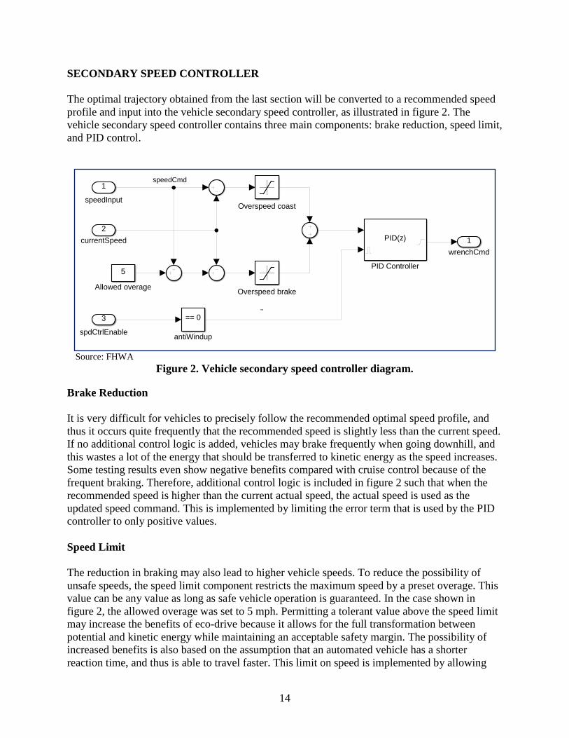
SECONDARY SPEED CONTROLLER The optimal trajectory obtained from the last section will be converted to a recommended speed profile and input into the vehicle secondary speed controller, as illustrated in figure 2. The vehicle secondary speed controller contains three main components: brake reduction, speed limit, and PID control.
Source: FHWA
Figure 2. Vehicle secondary speed controller diagram.
Brake Reduction It is very difficult for vehicles to precisely follow the recommended optimal speed profile, and thus it occurs quite frequently that the recommended speed is slightly less than the current speed. If no additional control logic is added, vehicles may brake frequently when going downhill, and this wastes a lot of the energy that should be transferred to kinetic energy as the speed increases. Some testing results even show negative benefits compared with cruise control because of the frequent braking. Therefore, additional control logic is included in figure 2 such that when the recommended speed is higher than the current actual speed, the actual speed is used as the updated speed command. This is implemented by limiting the error term that is used by the PID controller to only positive values. Speed Limit The reduction in braking may also lead to higher vehicle speeds. To reduce the possibility of unsafe speeds, the speed limit component restricts the maximum speed by a preset overage. This value can be any value as long as safe vehicle operation is guaranteed. In the case shown in figure 2, the allowed overage was set to 5 mph. Permitting a tolerant value above the speed limit may increase the benefits of eco-drive because it allows for the full transformation between potential and kinetic energy while maintaining an acceptable safety margin. The possibility of increased benefits is also based on the assumption that an automated vehicle has a shorter reaction time, and thus is able to travel faster. This limit on speed is implemented by allowing
1
speedInput
PID(z)
PID Controller
1wrenchCmd
2currentSpeed
3
spdCtrlEnable
== 0
antiWindup
Overspeed brake
5
Allowed overage
Overspeed coast
speedCmd

15
negative values for the error term that is used by the PID controller, but only if those values are more than the allowed overage below zero.
PID Control Initial testing revealed that a badly tuned PID controller is detrimental to eco-drive effectiveness, and even consumes more fuel than cruise control in some cases. This is because poorly tuned PID parameters may cause frequent acceleration and deceleration as the controller attempts to drive the vehicle at the target speed. Energy is wasted while braking and more fuel is wasted during accelerations. The parameters to be tuned are the proportional, integral, and derivative gains set in the Simulink PID block. The PID controller uses an error term that is the difference between the actual vehicle speed and the desired vehicle speed. The PID gains—kP, kI, and kD—are applied within the PID control block and a wrench effort command is generated. This command is applied to the lower-level vehicle controller. The wrench effort is a percentage between -100 and +100, where -100 to 0 percent loosely relates to braking in the range of -2.5 to 0 m/s2 and 0 to +100 percent loosely relates to acceleration in the range of 0 to 2.5 m/s2. To estimate the PID gains, a Simulink model is constructed and used to develop an initial set of values. Further PID tuning is performed through a manual tuning process during the field experiment. The first step is to gradually increase kP until an oscillation is observed in the output, then this value of kP is halved. Next, kI is increased enough to minimize the steady-state output error. Finally, kD is increased until the step response of the loop is acceptable. These parameters are usually particular to the dynamics of the experimental vehicle system, and different studies need to tune their own PID gains because of different vehicular dynamics. In a PID controller with nonzero kI, errors can accumulate while the PID controller is inactive, but the error signal is nonzero. This integrator windup is eliminated with an enable signal that is applied to the PID block. While the vehicle controller is inactive, the PID block is disabled and the output remains at zero. When the vehicle controller is activated, the PID operates normally. During the field experiment, each speed command is associated with a GPS coordinate and corresponding circular geofence along the roadway. The vehicle PC constantly checks to see if the current location is within a geofence. If so, the vehicle will execute the new speed command. If not, the vehicle will keep following the last speed command. The interval between these commands and the size of the geofence need to be predetermined. Also, there is delay between the time when GPS data are received by the antenna and the time when the vehicle finishes executing the speed command (including vehicle response delay). It is necessary to account for this delay by advancing the time at which commands are sent to the vehicle. The question is how far in advance a speed command should be given to the vehicle such that the vehicle’s speed can be close to the optimal speed (i.e. speed command) when arriving at certain location. Another parameter that needs to be determined is maximum acceleration (a required input for the vehicle control system). Initial experiments were conducted, and multiple scenarios with combinations of these parameters were tested.


17
CHAPTER 4. EXPERIMENTAL VEHICLE PLATFORM The CAV used in the field experiment is a part of FHWA’s automated vehicle fleet. Each vehicle was designed to be a complete research platform. (Please refer to Raboy and Ma (2017) for detailed introduction of the experimental vehicle platform.) Each research platform is outfitted with the following components:
• A proprietary longitudinal controller – a set of custom electronic control units (ECUs) that enable fully automatic control of vehicle acceleration and braking by integrating directly with the existing vehicle ACC system.
• A dSPACE MicroAutoBox (MAB) II controller – a specialized real-time computing platform that provides commands to the longitudinal controller (dSPACE, Inc., 2018). This is accessed via dSPACE ControlDesk through a MATLAB/Simulink library (MathWorks, 2018).
• An Arada LocoMate – a dedicated short-range communications (DSRC) onboard unit (OBU) that enables the transmission and reception of Basic Safety Messages (BSMs) (Arada Systems, 2018).
• A Linux-based, in-vehicle, secondary computer that integrates with the MAB. This computer gathers vehicle measures, operates the algorithms, and communicates with the human machine interface (HMI).
• PinPointTM – a special GPS device that fuses data from multiple sensors—including GPS—to create far more reliable positioning, velocity, orientation, and time metrics (Torc, 2018). This suite of sensors is always active, weighing all data to ensure accurate positioning even if GPS data are unavailable or inaccurate.
• TerraStar Service – a data services provider that enables accurate and efficient positioning solutions (TerraStar, 2018). The service uses a satellite-based positioning technique known as precise point positioning (PPP) that delivers an accuracy of a few centimeters globally using just a single receiver and without the need for a dedicated communications channel.
The base system configuration for the FHWA CAVs is shown in figure 3. At the center of the vehicle control system is the in-vehicle Linux PC. PinPoint™ transmits real-time, high-accuracy GPS data to the in-vehicle computer. The DSRC OBU broadcasts BSMs and receives other vehicles’ BSMs and transmits this information through the Linux PC. The long-range radar transmits object data to the Linux PC. The MAB receives data from Linux PC, including BSMs from other vehicles, roadside units (RSUs), and radar data. The MAB control commands are speed recommendations from the control algorithm embedded in Matlab Simulink, which are then injected into the vehicle CAN bus.

18
Source: FHWA Figure 3. Data flow of the vehicle control systems (Ma, Leslie, and Zhou, 2018).
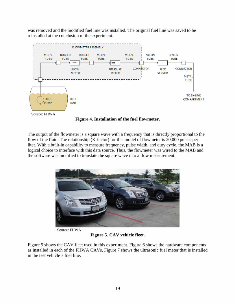
To enable the accurate measurement of fuel consumption, a fuel flow meter was installed to measure the amount of fuel delivered to the engine as a function of time. This flowmeter is accurate to better than ±1.0 percent over the whole 250:1 flow range, and repeatability is less than ±0.1 percent. The location was chosen based on the characteristics of the fuel system. This section of the fuel line is easily accessible, relatively low pressure (<100 psi), and away from the heat of the engine. The fuel system operates as a returnless system, meaning the in-tank fuel pump delivers the fuel required by the engine, and no fuel is returned to the tank. This simplifies the fuel flow measurement, but places additional restrictions on the location of the flowmeter. To ensure sufficient fuel pressure at the engine, the flowmeter was inserted upstream of the inline pressure sensor that is used to regulate the fuel pump. This would allow the vehicle’s closed-loop fuel pump controller to provide the appropriate fuel pressure at the engine. The modified fuel system is shown in figure 4. To simplify modifications to the vehicle, a replacement fuel line was purchased and modified with the flowmeter. Then the original fuel line
PID
Precision GNSS Receiver
Control Realtime Processor
GNSS: Global Navigation Satellite System
BSM: Basic Safety Message CAN: Controller Area
The vehicle’s data (e.g., speed, acceleration)
Radar
Radio In-Vehicle Computer
Vehicle CAN Bus System
The vehicle’s data (e.g., GPS) and other data (e.g., other vehicles’ BSM, RSU data)
19
was removed and the modified fuel line was installed. The original fuel line was saved to be reinstalled at the conclusion of the experiment.
Source: FHWA
Figure 4. Installation of the fuel flowmeter.
The output of the flowmeter is a square wave with a frequency that is directly proportional to the flow of the fluid. The relationship (K-factor) for this model of flowmeter is 20,000 pulses per liter. With a built-in capability to measure frequency, pulse width, and duty cycle, the MAB is a logical choice to interface with this data source. Thus, the flowmeter was wired to the MAB and the software was modified to translate the square wave into a flow measurement.
Source: FHWA
Figure 5. CAV vehicle fleet.
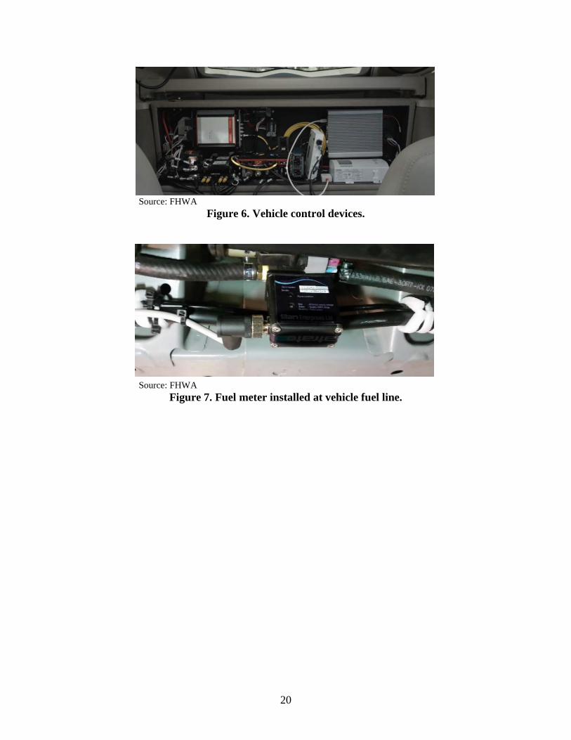
Figure 5 shows the CAV fleet used in this experiment. Figure 6 shows the hardware components as installed in each of the FHWA CAVs. Figure 7 shows the ultrasonic fuel meter that is installed in the test vehicle’s fuel line.
20
Source: FHWA
Figure 6. Vehicle control devices.
Source: FHWA
Figure 7. Fuel meter installed at vehicle fuel line.

21
CHAPTER 5. FIELD EXPERIMENT AND RESULTS EXPERIMENT DESIGN The experiment was conducted on seven rolling roadway segments in the States of Virginia and Maryland, with a total experimental mileage of around 47 miles. The types of terrain characterizing these segments vary from mildly rolling to very hilly. Power analyses were conducted on initial testing data using GPower statistical software (Faul et al., 2007) to determine the required number of runs. Twenty runs of data were collected by running a preset speed profile on one of the experimental segments. Corresponding fuel consumption data were recorded. The analysis results show that four, three, and two samples are needed for segment lengths of 2, 6, and 10 miles, respectively. Therefore, based on the segment length, four runs of data were collected and averaged in our experiment to account for certain random factors. Additionally, experimental runs on the same segment were collected on the same day to avoid confounding factors such as temperature, wind speed, and pavement condition that vary from day to day. Detailed roadway elevation profile data are not widely available for all roads. This study attempts to use the PinPoint device and PPP GPS service to collect elevation data. This method is preferred in the future, especially when all vehicles can be equipped with such advanced sensors. Note that this roadway profile information is usually collected through roadway survey and design documents from State DOT construction divisions, and are usually only available for newly constructed, major roads. However, given that roadway geometry data collected via connected vehicle technology are much more accessible than those from design/survey documents, it is believed that CV geometry data are more likely to be used as input for future eco-drive applications than survey data. Therefore, this experiment purposefully uses CV geometry data as inputs. It is one of the many design elements this experiment adopts to ensure the eco-drive application is tested under the most realistic environment. In the experiment, two scenarios are tested:
Baseline: The benchmark is regular cruise control with cruising speeds set to corresponding roadway speed limits. Eco-Drive: For eco-drive scenarios, vehicles will be given an optimal speed profile and will be controlled by the secondary speed controller in real time to follow the recommended speeds.
Fuel consumption was recorded, and the set of parameters that yield the lowest fuel consumption were selected (speed commands are given 13 meters (45 feet) in advance, geofence size/radius = 2 meters, maximum acceleration = 1 meter/sec,2 and speed command interval = 10 meters).

22
ROADWAY PROFILE DATA VALIDATION Detailed roadway elevation profile data are not widely available for all roads. This study attempts to use the PinPoint device and PPP GPS service to collect elevation data. This method is anticipated to be preferred in the future, especially when all vehicles can be equipped with such advanced sensors. Vehicle elevation data were compared with the ground truth elevation profile obtained from construction design and survey. The accuracy of the enhanced GPS data was then validated. The absolute value of elevation generally stays within a 3 percent error. Notably, this inaccuracy is mostly because of systematic errors, and the relative error reach is within 1 percent after a certain level of data smoothing. This confirms the validity of using such advanced GPS services for roadway profile data collection. ANALYSIS METHODOLOGY AND RESULTS Experimental data were analyzed at the segment and subsegment level to derive insights into the effectiveness of eco-drive. The subsegment level analysis compared average fuel consumption of baseline and eco-drive runs at each of the seven sites. Understanding of general eco-drive performance was obtained through close examination of vehicle speed, acceleration, brake status, brake percentages, and instantaneous fuel consumption profiles. The segment-level analysis, however, does not reveal actual contributors to differences in fuel saving. Therefore, subsegment-level analysis was performed by applying linear models. Variables describing the subsegment characteristics were extracted, and a linear model was established to reveal the impacts of different characteristics on fuel saving potential. Segment Data Analysis Figures 8(a) and (b) demonstrate actual speed data collected from two experimental runs (eco-drive and baseline) on Georgetown Pike as compared to commanded speed. The blue solid line shows the actual speed profile and the red dotted line shows the modified speed commands from the real-time secondary controller. The yellow dashed line is the actual speed profile when the vehicle tried to follow the speed commands (red dotted line). It can be seen from figure 8(a) that the vehicle can generally follow the speed commands closely even on this rolling terrain. At 1500 meters, the data between two black bars are removed from the fuel consumption calculation because there is a traffic light at which the vehicle stops during some runs. Figure 8(b) shows the baseline scenario in which speed commands were set to the speed limit of 35 mph (15.6 m/s). The actual speed profile (yellow dashed line) is compared with optimal speed commands. It shows that (adaptive) cruise control always tries to maintain the target speed, and thus it brakes frequently on downhill segments and applies the gas frequently on uphill segments. It is easy to predict that this behavior may result in extra fuel consumption. A closer look at the data in figure 8(a) reveals the smoothness of the vehicle trajectory, which is mostly because of a well-tuned PID control.

23
(a) Georgetown Pike example speed profile for eco-drive.
(b) Georgetown Pike example speed profile for baseline.
Figure 8. Speed Profile results at the segmental level for example runs (Source: FHWA).
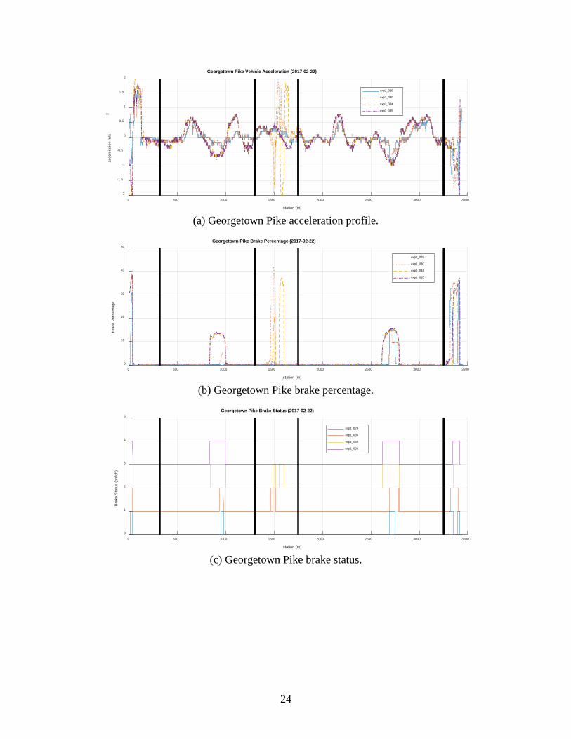
Figures 9(a) through (d) plot data from four experimental runs on vehicle acceleration, brake percentage, and brake status. Among these data, runs with labels of “exp1_029” and “exp1_030” are eco-drive runs, and those labeled “exp1_034” and “exp1_035” are baseline scenarios. The vehicle acceleration value and brake percentage of eco-drive runs are usually lower than the baseline runs. This is because the algorithm considers vehicle dynamics when generating the speed profile and the additional logic in the secondary real-time controller eliminates unnecessary braking relative to the baseline runs. The resulting fuel consumption benefits are reflected in figure 9(d). In many locations where acceleration was avoided, eco-drive runs consume much less fuel. Less braking and smaller brake percentages translate to a more effective transformation between potential and kinetic energy, thus less additional fuel is needed to provide the extra kinetic energy.
0 500 1000 1500 2000 2500 3000 3500
station (m)
0
5
10
15
20
Spee
d (m
/s)
Georgetown Pike Speeds for exp1_029 (2017-02-22)
Speed (profile)
Speed (to veh)
Speed (actual)
0 500 1000 1500 2000 2500 3000 3500
station (m)
0
5
10
15
20
Spee
d (m
/s)
Georgetown Pike Speeds for exp1_035 (2017-02-22)
Speed (profile)
Speed (to veh)
Speed (actual)
24
(a) Georgetown Pike acceleration profile.
(b) Georgetown Pike brake percentage.
(c) Georgetown Pike brake status.
0 500 1000 1500 2000 2500 3000 3500
station (m)
-2
-1.5
-1
-0.5
0
0.5
1
1.5
2
acce
lera
tion
m/s
2
Georgetown Pike Vehicle Acceleration (2017-02-22)
exp1_029
exp1_030
exp1_034
exp1_035
0 500 1000 1500 2000 2500 3000 3500
station (m)
0
10
20
30
40
50
Brak
e Pe
rcen
tage
Georgetown Pike Brake Percentage (2017-02-22)
exp1_029
exp1_030
exp1_034
exp1_035
0 500 1000 1500 2000 2500 3000 3500
station (m)
0
1
2
3
4
5
Brak
e St
atus
(on/
off)
Georgetown Pike Brake Status (2017-02-22)
exp1_029
exp1_030
exp1_034
exp1_035

25
(d) Georgetown Pike fuel consumption for multiple runs.
Note: exp1_029 and exp1_030 are eco-drive runs, and exp1_034 and exp1_035 are baseline runs. Figure 9. Experimental results at segmental level for example runs (Source: FHWA).
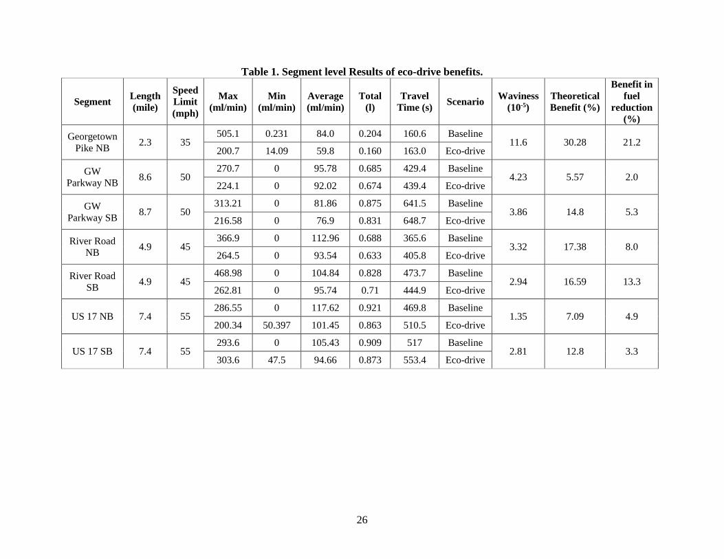
Table 1 details average results from each experimental site. Note that the travel times for the baseline and eco-drive scenarios are quite similar (mostly within a range of 5 percent) because the trajectory planning algorithm aims to maintain the same level of mobility while improving fuel consumption. The table also shows basic statistics as to instant fuel consumption throughout the experimental runs. As shown, the maximum instantaneous fuel consumption (mL/min) of the baseline runs is usually much larger than that of the eco-drive runs. The total fuel consumption savings vary significantly, ranging from 2 percent to more than 20 percent. This result is expected because fuel use is highly dependent on attributes of the terrain, such as hill length and slope. The roadway profile of Georgetown Pike NB consists of constant, continuous uphill and downhill segments with steep grades (4–8 percent), and thus, logically, there is greater room for improvement. For roadway segments like GW Parkway NB, the savings are relatively small because the roadway vertical profile is mild and it includes a flat subsegment that generates very small fuel consumption differences between the baseline and eco-drive scenarios. Additional analysis at the subsegment level is needed to understand exactly what impacts fuel consumption benefits. The algorithm speed commands are generated offline using a vehicle model and then fed to the vehicle longitudinal controller. To account for differences between the vehicle model and the actual vehicle (load, engine wear, transmission state, etc.) the actual vehicle speed was allowed to vary by 10 mph over or under the commanded speed. These differences, particularly the lack of direct control over transmission state, led to significant differences between the theoretical and measured fuel savings.
0 500 1000 1500 2000 2500 3000 3500
station (m)
0
50
100
150
200
250
300
350
400
450
fuel
con
sum
ptio
n (m
l/min
)
Georgetown Pike Fuel Consumption (2017-02-22)
exp1_029
exp1_030
exp1_034
exp1_035
26
Table 1. Segment level Results of eco-drive benefits.
Segment Length (mile)
Speed Limit (mph)
Max (ml/min)
Min (ml/min)
Average (ml/min)
Total (l)
Travel Time (s) Scenario Waviness
(10-5) Theoretical Benefit (%)
Benefit in fuel
reduction (%)
Georgetown Pike NB 2.3 35
505.1 0.231 84.0 0.204 160.6 Baseline 11.6 30.28 21.2
200.7 14.09 59.8 0.160 163.0 Eco-drive
GW Parkway NB 8.6 50
270.7 0 95.78 0.685 429.4 Baseline 4.23 5.57 2.0
224.1 0 92.02 0.674 439.4 Eco-drive
GW Parkway SB 8.7 50
313.21 0 81.86 0.875 641.5 Baseline 3.86 14.8 5.3
216.58 0 76.9 0.831 648.7 Eco-drive
River Road NB 4.9 45
366.9 0 112.96 0.688 365.6 Baseline 3.32 17.38 8.0
264.5 0 93.54 0.633 405.8 Eco-drive
River Road SB 4.9 45
468.98 0 104.84 0.828 473.7 Baseline 2.94 16.59 13.3
262.81 0 95.74 0.71 444.9 Eco-drive
US 17 NB 7.4 55 286.55 0 117.62 0.921 469.8 Baseline
1.35 7.09 4.9 200.34 50.397 101.45 0.863 510.5 Eco-drive
US 17 SB 7.4 55 293.6 0 105.43 0.909 517 Baseline
2.81 12.8 3.3 303.6 47.5 94.66 0.873 553.4 Eco-drive

27
Subsegment Data Analysis The subsegment-level analysis breaks down seven long segments listed in table 1 into many short subsegments, as illustrated in figure 10. The portion between two circles (one downhill and one uphill segment) is considered to be one subsegment. Fuel consumption savings were calculated as eco-drive fuel ÷ baseline fuel −1. In order to understand what attributes contribute the most to fuel consumption savings, the following subsegment characteristics were extracted for each subsegment: subsegment fuel consumption; uphill length (length of the uphill subsegment); uphill rise (elevation change of the uphill subsegment); uphill average slope (average slope along the uphill subsegment); downhill length (length of the downhill subsegment); downhill rise (elevation change of the downhill subsegment); downhill average slope (average slope along the downhill subsegment); and speed limit (distance-based average speed limit of the subsegment). To simplify the analysis, the uphill and downhill slopes were approximated using a straight line between the high point and low point. This slope is shown in the figure as black dotted lines.
Source: FHWA
Figure 10. Illustration of subsegments of River Road NB profile.
Linear models were built to understand which roadway attributes contribute the most to fuel savings. Therefore, subsegment fuel consumption is the response variable, and others are used as predictors. In addition, attributes of the prior and following subsegments were also used as predictors. This is because the algorithm tends to consider the future rolling terrain profile and the remaining kinetic energy at the beginning of the current subsegment (or end of the prior subsegment). This is directly related to how much additional energy the vehicle needs to traverse the current subsegment. Many of these predictors can be correlated; therefore, careful variable selection was conducted using a stepwise method and trial-and-error model construction (by removing highly correlated variables as measured by the Pearson correlation coefficient). The model with the best Akaike information criterion (AIC) value and prediction accuracy on test datasets was selected. Also, the

28
final model presented below has been diagnosed and the response variable has been transformed using the box-cox method to ensure the assumptions of the linear models are satisfied. Table 2 shows the results of the linear models. Note that interaction effects are considered in the original model, but those effects were neither significant nor selected in this final model. The R-squared value of the overall model is 0.705, indicating that 70 percent of the variance of fuel consumption saving variation can be captured by this model. The fuel saving is calculated as eco-drive fuel ÷ baseline fuel −1, and therefore negative coefficients indicate more fuel saving. Uphill lengths of the current subsegment positively impact the fuel saving benefits, mostly because the secondary controller limits the acceleration value to 1 meter/sec2, and the baseline manufacturer (adaptive) cruise control usually uses large acceleration values on long hills to maintain cruising speed. Subsegment waviness, as calculated using equation 24, is introduced to quantify the extent of waviness of a subsegment. Equation 25 adds waviness of all subsegments together to calculate overall waviness of a road segment, and table 1 shows these values for each experimental segment. The correlation between waviness and savings is generally minimal, except data for Georgetown Pike, where a large waviness value accompanies a large fuel savings. Otherwise, waviness cannot be directly correlated to fuel savings when the waviness values are similar, and this indicates that more complex relationship between the geometry and fuel savings may exist that are not captured in the linear model used in this paper to describe that relationship.
(24)
(25)
Where 𝑤𝑤𝑀𝑀 = the waviness of subsegment 𝑀𝑀. 𝑔𝑔𝑀𝑀𝑢𝑢 = average slope uphill. 𝑔𝑔𝑀𝑀𝑑𝑑 = average slope downhill. 𝑙𝑙𝑀𝑀 = subsegment length. 𝑊𝑊 = overall segment waviness. L = the overall length of the route.
Uphill length and average slope of the prior subsegment negatively impact savings. This result is expected because the large values of these two attributes mean that the vehicle can retain less kinetic energy when it climbs to the beginning of current subsegment. Meanwhile, the longer downhill length of the prior subsegment clearly results in larger benefits because the vehicle can accumulate more kinetic energy. Both the downhill and the uphill length of the next subsegment also significantly impact the actual saving of the current subsegment. It is difficult to obtain an intuitive explanation of the positive or negative impacts because, logically, the downstream subsegment should not impact upstream fuel consumption. This result, however, proves that the algorithm considers future rolling terrain when optimizing the speed profile, and it confirms the predictive nature of the algorithm.
𝑤𝑤𝑀𝑀 = (𝑔𝑔𝑀𝑀𝑢𝑢 − 𝑔𝑔𝑀𝑀𝑑𝑑)
𝑊𝑊 =1𝐿𝐿�𝑤𝑤𝑀𝑀𝑀𝑀

29
The linear model can also be used to roughly estimate the benefits of eco-drive for any roadway segment. This is a useful tool for traffic management centers because they would only want to control vehicle speeds or provide recommended speed profiles for eco-drive on roadways where large benefits can be generated. Traffic management centers can initially use this model to identify all these potential roadway segments where eco-drive is desired, and the list of these segments can always be updated later when real fuel data are collected.
Table 2. Subsegment level Results of eco-drive benefits. Variable Name Coefficient
Estimate Standard
Error t-Value p-Value
(Intercept) 4.87E+00 8.38E-01 5.809 1.35E-05 ***
Uphill length (1) -2.07E-04 4.64E-05 -4.454 0.000272 ***
Uphill average slope (1) -4.60E+00 2.86E+00 -1.612 0.123507
Downhill length (1) -9.91E-05 6.93E-05 -1.431 0.168774
Downhill average slope (1) 3.55E+00 3.01E+00 1.18 0.25241
Speed limit (1) -7.83E-02 1.76E-02 -4.445 0.000278 ***
Uphill length (0) 9.69E-05 4.48E-05 2.162 0.043586 *
Uphill average slope (0) 7.94E+00 3.09E+00 2.572 0.018649 *
Downhill length (0) -1.72E-04 6.36E-05 -2.708 0.013959 *
Uphill length (2) -1.66E-04 4.86E-05 -3.421 0.002868 **
Downhill length (2) 2.03E-04 1.03E-04 1.967 0.063947 .
R-squared = 0.69; F test p-value = 0.0035 a (1), (0) and (2) indicates ego, prior, and next subsegments. b Significance codes: 0: ‘***’; 0.001: ‘**’; 0.01: ‘*’; 0.05: ‘.’; 0.1; ‘ ’: 1. The linear regression model is expressed in equation 26.
(26)
Where βi = the coefficient estimate. xi = the corresponding variable. i ranges from 1 to the number of variables (in this case, i = {1, …, 10}).
%𝐶𝐶𝑎𝑎𝑣𝑣𝑀𝑀𝑚𝑚𝑔𝑔𝐶𝐶 = 𝛽𝛽0 + �𝛽𝛽𝑀𝑀𝑥𝑥𝑀𝑀𝑀𝑀


31
CHAPTER 6. CONCLUSIONS AND FUTURE RESEARCH This study proposes an eco-drive approach that consists of two speed controllers used in our experiment. The first is an upper-level controller that is responsible for trajectory planning to generate optimal speed profiles. The algorithm using the RPMP is computationally efficient and applicable in real time. The secondary controller adjusts speed commands in real time for enhanced performance and contains a typical PID controller for vehicle speed following. This study further tests these controllers and algorithms in real-world scenarios using an innovative CAV platform to better understand the algorithm performance. The proposed eco-drive system is compared against conventional constant speed cruise control on a total of seven road segments over 47 miles. The number of repetitions for each test is confirmed by statistical tests. The results confirm the fuel saving benefits of eco-drive. Experimental data show that more than 20 percent of fuel consumption can be saved on certain terrains. This research also breaks down test segments into shorter subsegments for further statistical analysis. Detailed investigation reveals the following major findings:
• The benefit of the proposed eco-drive system ranges from 3.3 percent to 21.2 percent. The magnitude of benefit is affected by hill length and slope grade.
• Conventional constant speed cruise control is fuel inefficient. It tends to apply gas on the uphill segment and then brake on the downhill segment. Hence, the replacement of conventional cruise control with the proposed eco-drive system on rolling terrains is very beneficial.
• Eco-drive reduces the amount of acceleration, leading to less braking. Less braking and smaller brake percentages translate to a more effective transformation between potential and kinetic energy, thus less additional fuel is needed to provide the extra kinetic energy.
• Detailed analysis through linear models also reveals the main contributors to the fuel savings potentially obtained from eco-drive. This conclusion can enable a rough estimate of the fuel saving potential of given roadways and help State DOTs to identify roadways where V2I-enabled eco-drive should be implemented.
The linear model can also be used to roughly estimate the benefits of eco-drive for any roadway segments. This model can enable rough estimation of the fuel saving potential of given roadways and help State DOTs to identify locations where eco-drive should be implemented. The algorithm and the experiment can also support OEMs in developing and marketing this technology to reduce fuel consumption and emissions in the future. In terms of suggested future studies, there are many directions in which to build from this study.
1. Field data on more experimental sites can be collected to examine eco-drive performance on a wide range of terrain conditions, and then more detailed subsegment analysis can be conducted.

32
2. Advanced algorithms may also consider the existence of a front vehicle (via vehicle-to-vehicle information) and downstream traffic congestion through addition of a speed harmonization component to the algorithm (Ma et al., 2016).
3. The proposed algorithm used speed commands to control the vehicle and did not exert control over the vehicle transmission. The experiment may be repeated with algorithm output that controls the transmission in addition to speed or throttle and an experimental vehicle with the capability of accepting commands for transmission state.
4. The current optimization method for synthesizing the optimal vehicle speed doesn't consider the gear shift schedule. This will cause some inaccuracy in estimating the fuel efficiency improvement since engines can only work at the speed dictated by the transmission gear shift schedule. One suggestion is to include the nonlinear gear shift schedule in the optimization method.
5. To further improve the energy efficiency, co-optimization of the vehicle speed and the transmission gear shift schedule could be conducted simultaneously. This is different than the previous approach, where only the existing gear shift schedule was included in the optimization method.
6. The proposed algorithm relies on an approximate vehicle dynamics model, and thus actual vehicles may not follow the commanded speed profiles well. Incorporating machine learning and artificial intelligence components in future algorithms will allow vehicles to plan the most suitable trajectories for themselves by using data from earlier operations.
7. This study focused on the benefits to a single vehicle running the experimental eco-drive algorithm. Further research is still needed to study the impact that the subject vehicle has on the traffic following it, including automated and nonautomated vehicles.
33
APPENDIX
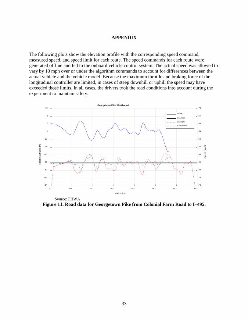
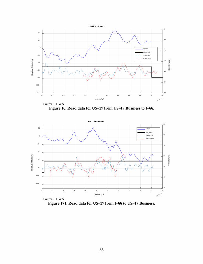
The following plots show the elevation profile with the corresponding speed command, measured speed, and speed limit for each route. The speed commands for each route were generated offline and fed to the onboard vehicle control system. The actual speed was allowed to vary by 10 mph over or under the algorithm commands to account for differences between the actual vehicle and the vehicle model. Because the maximum throttle and braking force of the longitudinal controller are limited, in cases of steep downhill or uphill the speed may have exceeded those limits. In all cases, the drivers took the road conditions into account during the experiment to maintain safety.
Source: FHWA
Figure 11. Road data for Georgetown Pike from Colonial Farm Road to I–495.
0 500 1000 1500 2000 2500 3000 3500
station (m)
-40
-35
-30
-25
-20
-15
-10
-5
0
5
10
Rel
ativ
e Al
titud
e (m
)
20
25
30
35
40
45
50
55
60
65
70
Spee
d (m
ph)
Georgetown Pike Westbound
altitude
speed limit
speed cmd
actual speed

34
Source: FHWA
Figure 12. Road data for George Washington Parkway Northbound from Key Bridge to I–495.
Source: FHWA
Figure 13. Road data for George Washington Parkway Southbound from I–495 to Key Bridge.
0 2000 4000 6000 8000 10000 12000 14000 16000
station (m)
-80
-60
-40
-20
0
20
40
60
80
Rel
ativ
e Al
titud
e (m
)
20
30
40
50
60
70
80
Spee
d (m
ph)
GW Pkwy Northbound
altitude
speed limit
speed cmd
actual speed
0 2000 4000 6000 8000 10000 12000 14000 16000
station (m)
-140
-120
-100
-80
-60
-40
-20
0
20
Rel
ativ
e Al
titud
e (m
)
20
30
40
50
60
70
80
Spee
d (m
ph)
GW Pkwy Southbound
altitude
speed limit
speed cmd
actual speed

35
Source: FHWA
Figure 14. Road data for River Road from Seven Locks Road to Seneca Road.
Source: FHWA
Figure 15. Road data for River Road from Seneca Road to Seven Locks Road.
0 2000 4000 6000 8000 10000 12000 14000 16000
station (m)
-80
-60
-40
-20
0
20
40
60
80
Rel
ativ
e Al
titud
e (m
)
20
30
40
50
60
70
80
Spee
d (m
ph)
River Rd Northbound
altitude
speed limit
speed cmd
actual speed
0 2000 4000 6000 8000 10000 12000 14000 16000
station (m)
-120
-100
-80
-60
-40
-20
0
20
40
Rel
ativ
e Al
titud
e (m
)
20
30
40
50
60
70
80
Spee
d (m
ph)
River Rd Southbound
altitude
speed limit
speed cmd
actual speed
36
Source: FHWA
Figure 16. Road data for US–17 from US–17 Business to I–66.
Source: FHWA
Figure 171. Road data for US–17 from I–66 to US–17 Business.
0 0.2 0.4 0.6 0.8 1 1.2 1.4 1.6 1.8 2 2.2
station (m) 10 4
-120
-100
-80
-60
-40
-20
0
20
40R
elat
ive
Altit
ude
(m)
30
40
50
60
70
80
90
Spee
d (m
ph)
US-17 Northbound
altitude
speed limit
speed cmd
actual speed
0 0.2 0.4 0.6 0.8 1 1.2 1.4 1.6 1.8 2 2.2
station (m) 10 4
-120
-100
-80
-60
-40
-20
0
20
Rel
ativ
e Al
titud
e (m
)
30
40
50
60
70
80
90
Spee
d (m
ph)
US-17 Southbound
altitude
speed limit
speed cmd
actual speed

37
ACKNOWLEDGMENTS This study is funded by the U.S. Department of Transportation (Project Number: DTFH61-12-D-00030/007). The work was conducted using the vehicle fleet and connected vehicle facility at the FHWA’s Turner-Fairbank Highway Research Center.


39
REFERENCES Arada Systems (2018). “LocoMate Classic On Board Unit OBU-200” (website). Available
online: http://www.aradasystems.com/locomate-obu/, last accessed January 25, 2018.
Boriboonsomsin, Kanok, and Matthew Barth (2009). "Impacts of road grade on fuel consumption and carbon dioxide emissions evidenced by use of advanced navigation systems." Transportation Research Record: Journal of the Transportation Research Board 2139: 21–30.
Dresner, K. and P. Stone (2008). “A multiagent approach to autonomous intersection management.” Journal of Artificial Intelligence Research, vol. 31: 591–656.
dSPACE, Inc (2018. “What’s new in the dSPACE products world.” (website). Available online: https://www.dspace.com/en/inc/home.cfm, last accessed January 25, 2018.
Faul, F., Erdfelder, E., Lang, A.G., and Buchner, A (2007). “G*Power 3: A flexible statistical power analysis program for the social, behavioral, and biomedical sciences.” Behavior Research Methods, 39: 175–191.
Hellström, Erik, Jan Åslund, and Lars Nielsen (2010). "Design of an efficient algorithm for fuel-optimal look-ahead control." Control Engineering Practice 18.11: 1318–1327.
Hu, Jia, et al. (2016). “Integrated optimal eco-driving on rolling terrain for hybrid electric vehicle with vehicle-infrastructure communication reference.” Transportation Research Part C, Vol. 68: 228–244.
Hu, J., Park, B. B., and Lee, Y. J (2015). “Coordinated transit signal priority supporting transit progression under connected vehicle technology.” Transportation Research Part C: Emerging Technologies, 55: 393–408.
Hu, S. R. and J.P. Lin (2013). “Effects of Three Advanced Devices on Crash and Gate Breaking Prevention at Highway-Railroad Grade Crossings.” Transportation Research Record: Journal of the Transportation Research Board: 109–117.
Ma, J., Leslie, E. and Zhou, F (2018). “Eco-Drive Experiment on Rolling Terrain for Fuel Consumption Optimization,” Report No. FHWA-HRT-18-010, FHWA, Washington, DC. Obtained from https://www.fhwa.dot.gov/publications/research/operations/18010/18010.pdf, last accessed January 23, 2018.
Ma, J., Li, X., Shladover, S., Rakha, H., Xiao-Yun, LU, Jagannathan, R., and Dailey, D (2016). “Freeway Speed Harmonization.” IEEE Transactions on Intelligent Vehicles, vol. 1, issue 1: 1–11.
40
Ma, J., Li, X., Zhou, F., Hu, J., and Park, B. B (2017). “Parsimonious shooting heuristic for trajectory design of connected automated traffic, part II: Computational issues and optimization.” Transportation Research Part B: Methodological, 95: 421–441.
Malakorn, K. J. and B. Park (2010). “Assessment of mobility, energy, and environment impacts of intellidrive-based Cooperative Adaptive Cruise Control and Intelligent Traffic Signal control,” Proc. 2010 IEEE International Symposium on Sustainable Systems and Technology (ISSST), Arlington, VA.
MathWorks (2018). “Simulation and Model-Based Design” (website). Available online: https://www.mathworks.com/products/simulink.html, last accessed January 25, 2018.
Park, H. and B. Smith (2012). “Investigating Benefits of IntellidriveSM in Freeway Operations-Lane Changing Advisory Case Study,” Journal of Transportation Engineering, vol 138, issue 9: 1113–1122.
Park, Sangjun, and Hesham Rakha (2006). "Energy and environmental impacts of roadway grades." Transportation Research Record: Journal of the Transportation Research Board 1987: 148–160.
Raboy, K., Ma, J., Stark, J., Zhou, F., Rush, K., and Leslie, E. (2017). “Cooperative Control for Lane Change Maneuvers with Connected Automated Vehicles: A Field Experiment.” Presentation, Transportation Research Board 96th Annual Meeting, Washington, DC, January 8–12, 2017. Paper no. 17-05142.
Sivaraman, S., M. M. Trivedi, M. Tippelhofer, and T. Shannon (2013). “Merge recommendations for driver assistance: A cross-modal, cost-sensitive approach,” in Proceedings of IEEE Intelligent Vehicles Symposium (IV): 411–416.
TerraStar (2018). “TerraStar” (website). Available online: http://www.terrastar.net, last accessed January 25, 2018.
Torc (2018). “Pinpoint: Multifaceted positioning for revolutionary location accuracy” (website). Available online: https://torc.ai/pinpoint/, last accessed January 25, 2018.
Van Arem, B., C. J. G. Van Driel, and R. Visser (2006). “The impact of Co-operative Adaptive Cruise Control on traffic flow characteristics,” IEEE Transactions on Intelligent Transportation Systems, vol. 7, no. 4: 429–436.
Vugts, R., et al (2010). “String-stable CACC design and experimental validation.” IEEE Transactions on Vehicular Technology, vol. 59, no. 9: 4268–4279.
Zhou, F., Li, X., & Ma, J. (2017). “Parsimonious shooting heuristic for trajectory design of connected automated traffic part I: Theoretical analysis with generalized time geography.” Transportation Research Part B: Methodological, 95: 394–420.