ecoe 554 machine learning - university of texas at dallaskoÇ university ecoe 554 machine learning...
TRANSCRIPT

KOÇ UNIVERSITY
ECOE 554 Machine Learning
Homework 4
Emrah ÇEM, 20081040
12/2/2009
In this homework, I used Boston Housing data and applied Linear Regression, Ridge Regression and Polynomial Regression algorithms to that data. Moreover, I created artificial data using PRTools, and applied linear, ridge and lasso regression algorithms to that data.
This homework has 2 part, in the first Boston Housing data was used. In the second part, artificial data was
created using PRTools.
PART1- BOSTON HOUSING DATA
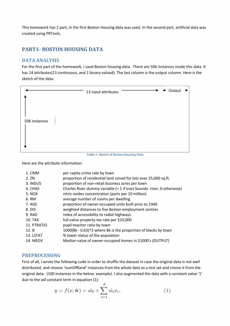
DATA ANALYSIS For the first part of the homework, I used Boston housing data. There are 506 instances inside this data. It
has 14 attributes(13 continuous, and 1 binary-valued). The last column is the output column. Here is the
sketch of the data:
Table 1- Sketch of Boston Housing Data
Here are the attribute information:
1. CRIM per capita crime rate by town 2. ZN proportion of residential land zoned for lots over 25,000 sq.ft. 3. INDUS proportion of non-retail business acres per town 4. CHAS Charles River dummy variable (= 1 if tract bounds river; 0 otherwise) 5. NOX nitric oxides concentration (parts per 10 million) 6. RM average number of rooms per dwelling 7. AGE proportion of owner-occupied units built prior to 1940 8. DIS weighted distances to five Boston employment centres 9. RAD index of accessibility to radial highways 10. TAX full-value property-tax rate per $10,000 11. PTRATIO pupil-teacher ratio by town 12. B 1000(Bk - 0.63)^2 where Bk is the proportion of blacks by town 13. LSTAT % lower status of the population 14. MEDV Median value of owner-occupied homes in $1000's (OUTPUT)
PREPROCESSING First of all, I wrote the following code in order to shuffle the dataset in case the original data is not well
distributed, and choose ‘numOfRand’ instances from the whole data as a test set and rmove it from the
original data. (100 instances in the below example). I also augmented the data with a constant value ‘1’
due to the w0 constant term in equation (1):
13 input attributes
506 instances
Output

I achieved those preprocessing operations by the following code:
numOfRand=100;
M=dlmread('housing.data');
[m,n]=size(M);
X=zeros(m,n);
X(:,1)=1;
X(:,2:n)=M(:,1:n-1);
y=M(:,n);
%shuffling indexes
ix = randperm(m);
X=X(ix,:);
y=y(ix,:);
input=X(1:numOfRand,:);
output=y(1:numOfRand);
X=X(numOfRand+1:end,:);
y=y(numOfRand+1:end);
As a result, I have 100 randomly chosen items as test set, and the remaining data set after calling this function. I call
this method only once to get reasonable results.
REGRESSION ALGORITHMS
Linear Regression
In standart linear regression X-y dependence is modeled as following:
where,
I started by writing 3 useful functions:
-A function(both for Linear and Ridge Regression) that takes as input a set of training data X={x1, x2,..., xn},
Y={y1, y2,..., yn,} and produces as output an estimate of the optimal weight vector.
function[w]=ridgeRegressionWeights(X,Y,lambda)
w=(X'*X+lambda*eye(size(X,2)))\(X'*Y);
end
function[w]=linearRegressionWeights(X,Y)
w=(X'*X)\(X'*Y);
end

-A function that takes a weight vector w and a case x and produces a prediction of the associated value y.
function[y]=predictor(w,x)
y=w'*x;
end
-A function that takes as input a training set of input and output values and a test set of input and output
values and returns the mean squared training error and the mean squared test error.
%given training set input-output, and test set input-output, %calculates
training and test set MSE (for linear and ridge %regression)
function [rtrainerr,rtesterr,ltrainerr,ltesterr]=
errorCalculator(trainin, trainout,testin, testout)
%regularization constant is chosen as 10^-6
w=ridgeRegressionWeights(trainin,trainout,10^-6);
w2=linearRegressionWeights(trainin,trainout);
rtrainerr=meanSquaredError(trainin,trainout,w);
rtesterr=meanSquaredError(testin,testout,w);
ltrainerr=meanSquaredError(trainin,trainout,w2);
ltesterr=meanSquaredError(testin,testout,w2);
end
%Given the input data outputs and the estimated weight vector, calculates
%the MSE
function [err]=meanSquaredError(X,y,w)
sum=0;
for i=1:size(X,1)
xi=X(i,:)';
guess=predictor(w,xi);
diff(i)=(guess-y(i));
sum=sum+diff(i)*diff(i);
end
err=sum/size(X,1);
end
Results for Linear Regression and Ridge Regression
I tried different values for regularization parameter ‘a’ and compared Linear regression and Ridge
regression. I run 50 experiments and took average of them to take logcal results. Here are the results:
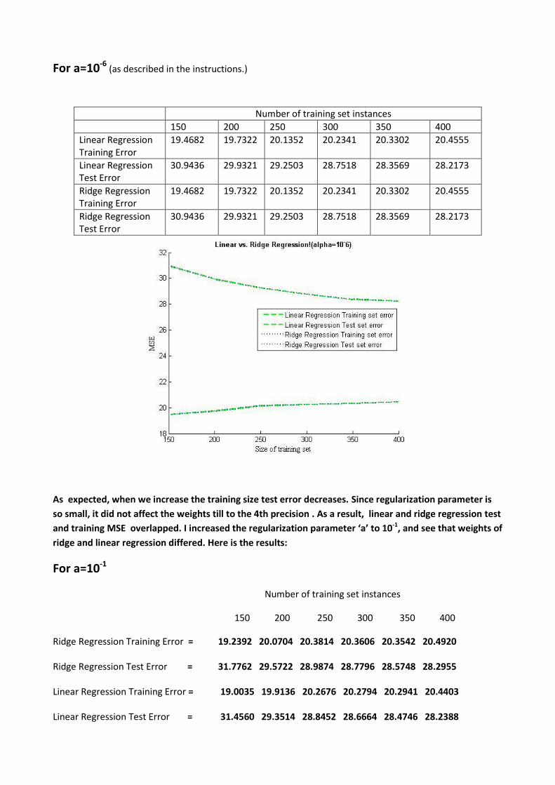
For a=10-6 (as described in the instructions.)
Number of training set instances
150 200 250 300 350 400
Linear Regression Training Error
19.4682 19.7322 20.1352 20.2341 20.3302 20.4555
Linear Regression Test Error
30.9436 29.9321 29.2503 28.7518 28.3569 28.2173
Ridge Regression Training Error
19.4682 19.7322 20.1352 20.2341 20.3302 20.4555
Ridge Regression Test Error
30.9436 29.9321 29.2503 28.7518 28.3569 28.2173
As expected, when we increase the training size test error decreases. Since regularization parameter is
so small, it did not affect the weights till to the 4th precision . As a result, linear and ridge regression test
and training MSE overlapped. I increased the regularization parameter ‘a’ to 10-1, and see that weights of
ridge and linear regression differed. Here is the results:
For a=10-1
Number of training set instances
150 200 250 300 350 400
Ridge Regression Training Error = 19.2392 20.0704 20.3814 20.3606 20.3542 20.4920 Ridge Regression Test Error = 31.7762 29.5722 28.9874 28.7796 28.5748 28.2955 Linear Regression Training Error = 19.0035 19.9136 20.2676 20.2794 20.2941 20.4403 Linear Regression Test Error = 31.4560 29.3514 28.8452 28.6664 28.4746 28.2388
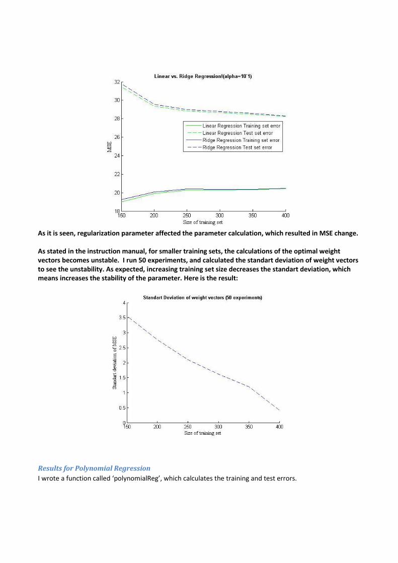
As it is seen, regularization parameter affected the parameter calculation, which resulted in MSE change. As stated in the instruction manual, for smaller training sets, the calculations of the optimal weight vectors becomes unstable. I run 50 experiments, and calculated the standart deviation of weight vectors to see the unstability. As expected, increasing training set size decreases the standart deviation, which means increases the stability of the parameter. Here is the result:
Results for Polynomial Regression
I wrote a function called ‘polynomialReg’, which calculates the training and test errors.
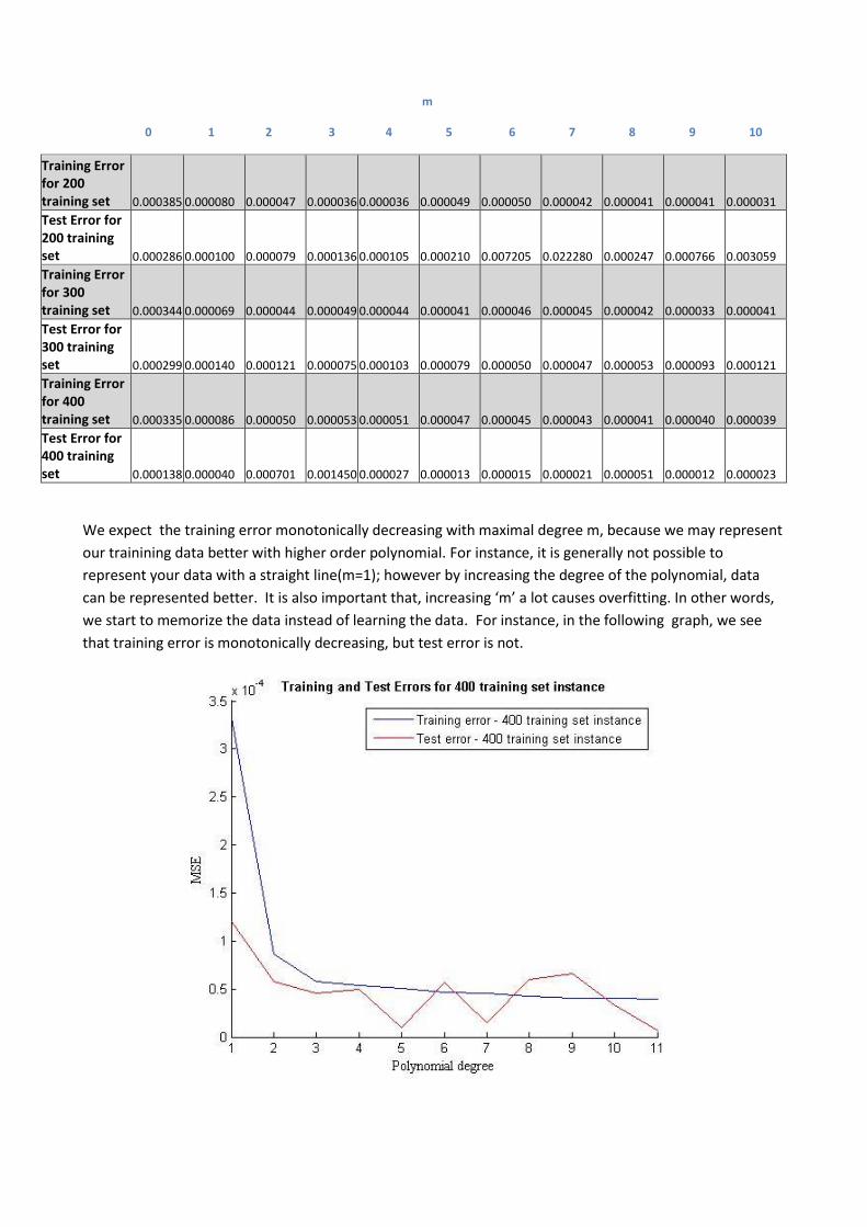
m
0 1 2 3 4 5 6 7 8 9 10
Training Error for 200 training set 0.000385 0.000080 0.000047 0.000036 0.000036 0.000049 0.000050 0.000042 0.000041 0.000041 0.000031
Test Error for 200 training set 0.000286 0.000100 0.000079 0.000136 0.000105 0.000210 0.007205 0.022280 0.000247 0.000766 0.003059
Training Error for 300 training set 0.000344 0.000069 0.000044 0.000049 0.000044 0.000041 0.000046 0.000045 0.000042 0.000033 0.000041
Test Error for 300 training set 0.000299 0.000140 0.000121 0.000075 0.000103 0.000079 0.000050 0.000047 0.000053 0.000093 0.000121
Training Error for 400 training set 0.000335 0.000086 0.000050 0.000053 0.000051 0.000047 0.000045 0.000043 0.000041 0.000040 0.000039
Test Error for 400 training set 0.000138 0.000040 0.000701 0.001450 0.000027 0.000013 0.000015 0.000021 0.000051 0.000012 0.000023
We expect the training error monotonically decreasing with maximal degree m, because we may represent
our trainining data better with higher order polynomial. For instance, it is generally not possible to
represent your data with a straight line(m=1); however by increasing the degree of the polynomial, data
can be represented better. It is also important that, increasing ‘m’ a lot causes overfitting. In other words,
we start to memorize the data instead of learning the data. For instance, in the following graph, we see
that training error is monotonically decreasing, but test error is not.

PART2- ARTIFICAL DATA I created 5 artificial datasets with 10, 20, 40, 60, 100 instances, a test data with 30 instances and a
validation set with 30 instances using gendatsinc.
A1=gendatsinc(70); %Create 70 data points
A2=gendatsinc(80); %Create 80 data points
A3=gendatsinc(100); %Create 100 data points
A4=gendatsinc(120); %Create 120 data points
A5=gendatsinc(160); %Create 160 data points
[tr1,test1] = gendat(A1, 4/7); %Split 70 into 40(train) and 30(test)
[tr2,test2] = gendat(A2, 5/8); %Split 80 into 50(train) and 30(test)
[tr3,test3] = gendat(A3, 7/10);%Split 100 into 70(train) and 30(test)
[tr4,test4] = gendat(A4, 9/12);%Split 120 into 90(train) and 30(test)
[tr5,test5] = gendat(A5, 13/16);%Split 70 into 40(train) and 30(test)
[train1,valid1]=gendat(tr1, 1/4);%Split 40 into 10(train) and 30(val)
[train2,valid2]=gendat(tr2, 2/5);%Split 50 into 20(train) and 30(val)
[train3,valid3]=gendat(tr3, 4/7);%Split 70 into 40(train) and 30(val)
[train4,valid4]=gendat(tr4, 6/9);%Split 90 into 60(train) and 30(val)
[train5,valid5]=gendat(tr5, 10/13);%Split 130 into 100(train) and
%30(val)
As a result, I have the following datasets:
Number of Training Set Instances
Number of Validation Set Instances
Number of Test Set Instances
Dataset1(train1,valid1,test1) 10 30 30
Dataset2(train2,valid2,test2) 20 30 30
Dataset3(train3,valid3,test3) 40 30 30
Dataset4(train4,valid4,test4) 60 30 30
Dataset5(train5,valid5,test5) 100 30 30
Regression Algorithms There was only regularization parameter to optimize in all regression types. Actually, linearr had another
parameter N, which is order of polynomial. I tried different values for N, but I got the same test error.
Hence I did not include the results in the report.
Results for dataset with 10 training set instance
I optimized the regularization parameters using validation set. I tried regularization parameter
c={0.1,0.2,...,9.9,10}
for i = 1:100
YLin = train1*linearr([],0.1*i);
YRidge=train1*ridger([],0.1*i);
YLasso=train1*lassor([],0.1*i);
%optimize using validation set
LinValErrors(i) = valid1*YLin*testr;
RidgeValErrors(i) = valid1*YRidge*testr;

LassoValErrors(i) = valid1*YLasso*testr;
I calculated the errors for regression algorithms above, then I found on which regularization parameter(C) I
got the minimum error. Then I apply the optimized model to the test set and get the error values.
[LinMin_val,LinIndex] = min(LinValErrors);
LinModel = train1*linearr([],0.1*LinIndex); % model
LinError = test1*LinModel*testr; %MSE
[RidgeMin_val,RidgeIndex] = min(RidgeValErrors);
RidgeModel = train1*linearr([],0.1*RidgeIndex); % model
RidgeError = test1*RidgeModel*testr; %MSE
[LassoMin_val,LassoIndex] = min(LassoValErrors);
LassoModel = train1*linearr([],0.1*LassoIndex); % model
LassoError = test1*LassoModel*testr; %MSE
MSE
----------
linear regression (Optimized C=100) : 0.009320
ridge regression (Optimized C=1) : 0.010107
lasso regression (Optimized C=1) : 0.010107
Tablo 1
Right graph shows that, when regression parameter increases, MSE error
decreases in Linear Regression, but stays constant in Lasso and Ridge
regression.

Results for dataset with 20 training set instance
MSE
----------
linear regression (Optimized C=1) : 0.084001
ridge regression (Optimized C=100) : 0.082745
lasso regression (Optimized C=100) : 0.082745
Results for dataset with 40 training set instance MSE
-----------
linear regression (Optimized C=1) : 0.130758
ridge regression (Optimized C=100) : 0.134862
lasso regression (Optimized C=100) : 0.134862

Results for dataset with 60 training set instance
MSE
----------
linear regression (Optimized C=1) : 0.085123
ridge regression (Optimized C=100) : 0.085388
lasso regression (Optimized C=100) : 0.085388
Results for dataset with 100 training set instance MSE
----------
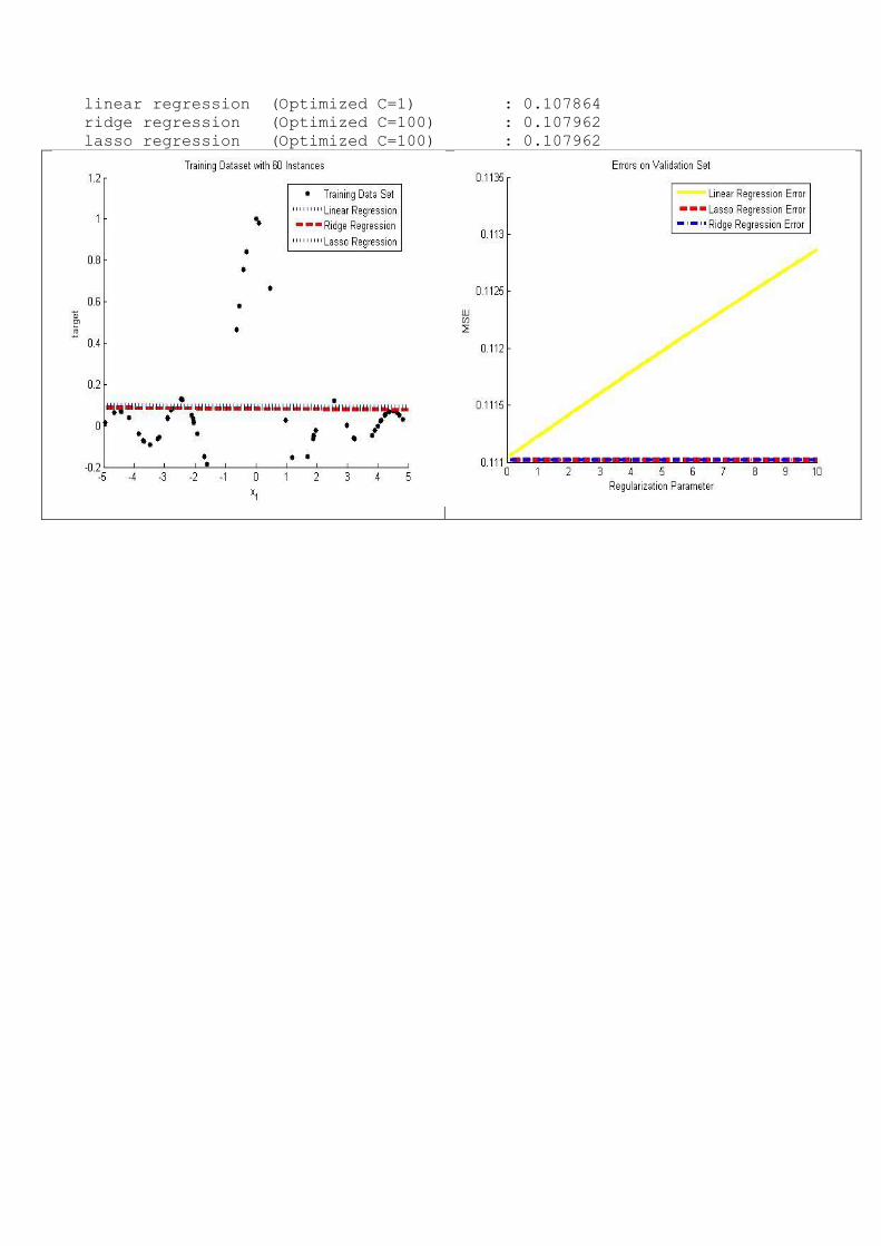
linear regression (Optimized C=1) : 0.107864
ridge regression (Optimized C=100) : 0.107962
lasso regression (Optimized C=100) : 0.107962