1981 - 14

ECOLOGICAL INVESTIGATIONS OF PETROLEUM PRODUCTION PLATFORMS

IN THE CENTRAL GULF OF MEXICO

VOLUME I-POL4UTANT FATE AND EFFECTS STUDIES

Part1-Background, Program Organization and Study Plan Part ~-Sedimen t) Physical Characterization Par~ 3-Orgapfc Chemical Analyses

I ~ -> _~r 4I! I \Editor:

1 C. A. Bedinger, Jr .

----P-r6gram Manager

Editorial Assistant :

'^--4,aura Z . Kirby

i 1

SOUTHWEST RESEARCH INSTITUTE SAN ANTONIO HOUSTON

DISCLAIMER

"This report has been reviewed by the Bureau of Land Management and approved for publication . Approval does not signify that the contents necessarily reflect the view and policies of the Bureau, nor does mention of wade names or commercial products constitute endorsement or recommendation for use."

This report is not available from the sponsor . A limited number of printed copies are available from Southwest Research Institute, 2200 W. Loop South, Suite 690, Houston, Texas 77027, Attention : Dr . C.A . Bedinger, Jr . Photostatic copies will be available from the National Technical Information Service .

ECOLOGICAL INVESTIGATIONS OF PETROLEUM PRODUCTION PLATFORMS IN THE

CENTRAL GULF OF MEXICO

Submitted to :

Bureau of Land Management, New Orleans OCS Attention: Frances Sullivan Hale Boggs Federal Building 500 Camp Street, Suite 841

New Orleans, Louisiana 70130

SwRI Project 01-52

In fulfillment of Contra ` .ti AA551-CT8-17

by:

Southwest Research Institute 6220 Culebra Road P.O . Drawer 28510

San Antonio, Texas 78284

1981

GUIDE TO USERS

This report is in six separate bindings:

1 VOLUME I -POLLUTANT FATE AND EFFECTS STUDIES Part 1 -Background, Program Organization and Study Plan Part 2 -Sediment Physical Characterization Part 3 -Organic Chemical Analyses

2 VOLUME I -POLLUTANT FATE AND EFFECTS STUDIES Part 4 -Trace Metals Studies in Sediment and Fauna Part S -Microbiology and Microbiological Processes

3 VOLUME I -POLLUTANT FATE AND EFFECTS STUDIES Part 6 -Benthic Biology Part 7 -Normal Histology and Histopathology of Benthic Inverte

brates and Demersal and Platform-Associated Pelagic Fishes

4 VOLUME I -POLLUTANT FATE AND EFFECTS STUDIES Part 8 -Summary Data Set

S VOLUME II -THE ARTIFICIAL REEF STUDIES

6 VOLUME III -EXECUTIVE SUMMARY

CONTENTS OF THIS BINDING

Page VOLUME I -POLLUTANT FATE AND EFFECT STUDIES

Part 1-Background, Program Organization and Study Plan 1 Part 2-Sediment Physical Characterization SS Part 3-Organic Chemical Analyses 133

A detailed Table of Contents for each part in this binding immediately follows the Title Page for that part.

VOLUME I-POLLUTANT FATE AND EFFECTS STUDIES Part 1-Background, Program Organization and Study Plan

by

C.A. Bedinger, Jr . Program Manager

Ralph E . Childers Data Manager

John W . Cooper Chief Scientist Shipboard Operations

Kay T. Kimball Data Synthesis Manager

Alan Kwok Research Scientist

Editor: C.A. Bedinger, Jr . Editorial Assistant: Laura Z. Kirby

Southwest Research Institute Department of Environmental Sciences

Division of Chemistry and Chemical Engineering 3600 Yoakum Boulevard Houston, Texas 77006

TABLE OF CONTENTS

Page I. HOW TO USE THIS REPORT.. . . . . . . . . . . . . . . . . . . . . . . . . . . . . . . . . . . . . . . . . . . . . . . . . . . . . . . . . . . . . . . . . . . . . . . . . . . . . . . . . . . . . . . . . . . . . . 1

A. Volume I, Pollutant Fate and Effects Studies .. . . . . . . . . . . . . . . . . . . . . . . . . . . . . . . . . . . . . . . . . . . . . . . . . . . . . . . . . . . . . . . . . . . . . 1 B. Volume II, Artificial Reef Studies . . . . . . . . . . . . . . . . . . . . . . . . . . . . . . . . . . . . . . . . . . . . . . . . . . . . . . . . . . . . . . . . . . . . . . . . . . . . . . . . . . . . 1 C. Volume III, The Executive Summary ... . . . . . . . . . . . . . . . . . . . . . . . . . . . . . . . . . . . . . . . . . . . . . . . . . . . . . . . . . . . . . . . . . . . . . . . . . . . . . 1

II . INTRODUCTION TO PART 1 . . . . . . . . . . . . . . . . . . . . . . . . . . . . . . . . . . . . . . . . . . . . . . . . . . . . . ., . . . . . . . . . . . . . . . . . . . . . . . . . . . . . . . . . . . . . . . . 3 A. Philosophy of the Study. . . . . . . . . . . . . . . . . . . . . . . . . . . . . . . . . . . . . . . . . . . . . . . . . . . . . . . . . . . . . . . . . . . . . . . . . . . . . . . . . . . . . . . . . . . . . . . . . 3 B. Legislative Authority Behind the Study... . . . . . . . . . . . . . . . . . . . . . . . . . . . . . . . . . . . . . . . . . . . . . . . . . . . . . . . . . . . . . . . . . . . . . . . . . . . 3 C. Objectives of the Study. . . . . . . . . . . . . . . . . . . . . . . . . . . . . . . . . . . . . . . . . . . . . . . . . . . . . . . . . . . . . . . . . . . . . . . . . . . . . . . . . . . . . . . . . . . . . . . . . . 3

1 . Objectives of the BLM OCS Environmental Studies Program . . . . . . . . . . . . . . . . . . . . . . . . . . . . . . . . . . . . . . . . . 3 2 . Objectives of the Central Gulf Platform Study . . . . . . . . . . . . . . . . . . ., . . . . . . . . . . . . . . . . . . . . . . . . . . . . . . . . . . . . . . . . 3

D. Relationship to Previous Studies . . . . . . . . . . . . . . . . . . . . . . . . . . . . . . . . . . . . . . . . . . . . ., . . . . . . . . . . . . . . . . . . . . . . . . . . . . . . . . . . . . . . . . 4

III . BACKGROUND INFORMATION ON THE LOUISIANA OCS .... . . . . . . . . . . . . . . . . . . . . . . . . . . . . . . . . . . . . . . . . . . . . . . . . S A. Physiography of the Louisiana OCS ... . . . . . . . . . . . . . . . . . . . . . . . . . . . . . . . . . . . . . . . . . . . . . . . . . . . . . . . . . . . . . . . . . . . . . . . . . . . . . . S

1 . Geology. . . . . . . . . . . . . . . . . . . . . . . . . . . . . . . . . . . . . . . . . . . . . . . . . . . . . . . . . . . . . . . . . . . . . . . . . . . . . . . . . . . . . . . . . . . . . . . . . . . . . . . . . . . . . S 2. Oceanography . . . . . . . . . . . . . . . . . . . . . . . . . . . . . . . . . . . . . . . . . . . . . . . . . . . . . . . . . . . . . . . . . . . . . . . . . . . . . . . . . . . . . . . . . . . . . . . . . . . . . 5

a. Introduction . . . . . . . . . . . . . . . . . . . . . . . . . . . . . . . . . . . . . . . . . . . . . . . . . . . . . . . . . . . . . . . . . . . . . . . . . . . . . . . . . . . . . . . . . . . . . . . S 6. Advective Processes.. . . . . . . . . . . . . . . . . . . . . . . . . . . . . . . . . . . . . . . . . . . . . . . . . . . . . . . . . . . . . . . . . . . . . . . . . . . . . . . . . . . . . 6

(1) Gulf of Mexico Circulation. . . . . . . . . . . . . . . . . . . . . . . . . . . ., . . . . . . . . . . . . . . . . . . . . . . . . . . . ., . . . . . . . . . ., 6 (2) Louisiana Shelf Circulation . . . . . . . . . . . . . . . . . . . . . . . . . . . . . . . . . . . . . . . . . . . . . . . . . . . . . . . . . . . . . . . . . . . . 7 (3) Dissolved Oxygen in the Waters of theStudy Area ... . . . . . . . . . . . . . . . . . . . . . . . . . . . . . . . . . . . . . 10 (4) Estimate of Petroleum Hydrocarbons in the Mississippi River Discharge ... . . . . . . . . 13

B. Petroleum and the Louisiana OCS. . . . . . . . . . . . . . . . . . . . . . . . . . . . . . . . . . . . . . . . . . . . . . . . . . . . . . . . . . . . . . . . . . . . . . . . . . . . . . . . . . . . 14 l . Historical Background of the Offshore Oil Industry in the Gulf of Mexico . . . . . . . . . . . . . . . . . . . . . . . . . 14 2. Historical Background of the Oil Industry Off Louisiana... . . . . . . . . . . . . . . . . . . . . . . . . . . . . . . . . . . . . . . . . . . . . 15 3. Economic Impact of the Oil Industry Off Louisiana ... . . . . . . . . . . . . . . . . . . . . . . . . . . . . . . . . . . . . . . . . . . . . . . . . . . 15 4 . Important Ecological Impacts of the Oil Industry Off Louisiana . . . . . . . . . . . . . . . . . . . . . . . . . . . . . . . . . . . . . . 15

a. Oil Spills on the Louisiana OCS. . . . . . . . . . . . . . . . . . . . . . . . . . . . . . . . . . . . . . . . . . . . . . . . . . . . . . . . . . . . . . . . . . . . . . . 16 b . The "Artificial Reef" Concept and Petroleum Pollution . . . . . . . . . . . . . . . . . . . . . . . . . . . . . . . . . . . . . . . 16

C. Literature Review of Studies Relevant to this Investigation .. . . . . . . . . . . . . . . . . . . . . . . . . . . . . . . . . . . . . . . . . . . . . . . . . . . . 17 l. The Offshore Ecology Investigation . . . . . . . . . . . . . . . . . . . . . . . . . . . . . . . . . . . . . . . . . . . . . . . . . . . . . . . . . . . . . . . . . . . . . . . . . . 17 2. Bureau of Land Management OCS Benchmark Studies .. . . . . . . . . . . . . . . . . . . . . . . . . . . . . . . . . . . . . . . . . . . . . . . . 17 3. Sources, Fate, and Effects of Petroleum Hydrocarbons in the Marine Environment . . . . . . . . . . . . . 18

a. Sources. . . . . . . . . . . . . . . . . . . . . . . . . . . . . . . . . . . . . . . . . . . . . . . . . . . . . . . . . . . . . . . . . . . . . . . . . . . . . . . . . . . . . . . . . . . . . . . . . . . . . . 18 b . Fate . . . . . . . . . . . . . . . . . . . . . . . . . . . . . . . . . . . . . . . . . . . . . . . . . . . . . . . . . . . . . . . . . . . . . . . . . . . . . . . . . . . . . . . . . . . . . . . . . . . . . . . . . . 18 c. Effects . . . . . . . . . . . . . . . . . . . . . . . . . . . . . . . . . . . . . . . . . . . . . . . . . . . . . . . . . . . . . . . . . . . . . . . . . . . . . . . . . . . . . . . . . . . . . . . . . . . . . . 19

D. Fisheries of the Louisiana OCS ... . . . . . . . . . . . . . . . . . . . . . . . . . . . . . . . . . . . . . . . . . . . . . . . . . . . . . . . . . . . . . . . . . . . . . . . . . . . . . . . . . . . . . 20 l. Delineation of the Segments of Louisiana Fisheries.. . . . . . . . . . . . . . . . . . . . . . . . . . . . . . . . . . . . . . . . . . . . . . . . . . . . . . 20 2. Delineation of Marine Fisheries .. . . . . . . . . . . . . . . . . . . . . . . . . . . . . . . . . . . . . . . . . . . . . . . . . . . . . . . . . . . . . . . . . . . . . . . . . . . . . . 21 3. Commercial Fisheries.. . . . . . . . . . . . . . . . . . . . . . . . . . . . . . . . . . . . . . . . . . . . . . . . . . . . . . . . . . . . . . . . . . . . . . . . . . . . . . . . . . . . . . . . . . . 21 4 . Sport Fisheries . . . . . . . . . . . . . . . . . . . . . . . . . . . . . . . . . . . . . . . . . . . . . . . . . . . . . . . . . . . . . . . . . . . . . . . . . . . . . . . . . . . . . . . . . . . . . . . . . . . . 21 S. Influence of Production Platforms on Fisheries.. . . . . . . . . . . . . . . . . . . . . . . . . . . . . . . . . . . . . . . . . . . . . . . . . . . . . . . . . . 22

a . Findings of the Buccaneer Oil Field Study . . . . . . . . . . . . . . . . . . . . . . . . . . . . . . . . . . . . . . . . . . . . . . . . . . . . . . . . . . 22 b. Unverified Influences.. . . . . . . . . . . . . . . . . . . . . . . . . . . . . . . . . . . . . . . . . . . . . . . . . . . . . . . . . . . . . . . . . . . . . . . . . . . . . . . . . . . 22

IV . PROGRAM ORGANIZATION .. . . . . . . . . . . . . . . . . . . . . . . . . . . . . . . . . . . . . . . . . . . . . . . . . . . . . . . . . . . . . . . . . . . . . . . . . . . . . . . . . . . . . . . . . . . . . 23 V. STUDY PLATFORMS AND CONTROL SITES . . . . . . . . . . . . . . . . . . . . . . . . . . . . . . . . . . . . . . . . . . . . . . . . . . . . . . . . . . . . . . . . . . . . . . . . 25

A. Selection Criteria for Study Sites.. . . . . . . . . . . . . . . . . . . . . . . . . . . . . . . . . . . . . . . . . . . . . . . . . . . . . . . . . . . . . . . . . . . . . . . . . . . . . . . . . . . . . 25 B. Location of the Study Area and Sites . . . . . . . . . . . . . . . . . . . . . . . . . . . . . . . . . . . . . . . . . . . . . . . . . . . . . . . . . . . . . . . . . . . . . . . . . . . . . . . . 25 C. List of Study Sites with Characteristics . . . . . . . . . . . . . . . . . . . . . . . . . . . . . . . . . . . . . . . . . . . . . . . . . . . . . . . . . . . . . . . . . . . . . . . . . . . . . . 25 D. Problems in Study Site Selection .. . . . . . . . . . . . . . . . . . . . . . . . . . . . . . . . . . . . . . . . . . . . . . . . . . . . . . . . . . . . . . . . . . . . . . . . . . . . . . . . . . . . . 30

1. Control Site Selection.. . . . . . . . . . . . . . . . . . . . . . . . . . . . . . . . . . . . . . . . . . . . . . . . . . . . . . . . . . . . . . . . . . . . . . . . . . . . . . . . . . . . . . . . . . . 30 2. Oxygen Depletion and Resultant Dead Bottoms... . . . . . . . . . . . . . . . . . . . . . . . . . . . . . . . . . . . . . . . . . . . . . . . . . . . . . . . . 30 3. Drilling and Workover Operations . . . . . . . . . . . . . . . . . . . . . . . . . . . . . . . . . . . . . . . . . . . . . . . . . . . . . . . . . . . . . . . . . . . . . . . . . . . .30 4. Underwater Obstructions and Satellite Platforms... . . . . . . . . . . . . . . . . . . . . . . . . . . . . . . . . . . . . . . . . . . . . . . . . . . . . . . 30 S. Petroleum Industry Cooperation . . . . . . . . . . . . . . . . . . . . . . . . . . . . . . . . . . . . . . . . . . . . . . . . . . . . . . . . . . . . . . . . . . . . . . . . . . . . . 31

VI. SCOPE OF WORK .... . . . . . . . . . . . . . . . . . . . . . . . . . . . . . . . . . . . . . . . . . . . . . . . . . . . . . . . . . . . . . . . . . . . . . . . . . . . . . . . . . . . . . . . . . . . . . . . . . . . . . . . . . . 33 A. Field Sampling Program . . . . . . . . . . . . . . . . . . . . . . . . . . . . . . . . . . . . . . . . . . . . . . . . . . . . . . . . . . . . . . . . . . . . . . . . . . . . . . . . . . . . . . . . . . . . . . . . 33

1. Sampling Cruises . . . . . . . . . . . . . . . . . . . . . . . . . . . . . . . . . . . . . . . . . . . . . . . . . . . . . . . . . . . . . . . . . . . . . . . . . . . . . . . . . . . . . . . . . . . . . . . . . 33 2. SamplingPattems . . . . . . . . . . . . . . . . . . . . . . . . . . . . . . . . . . . . . . . . . . . . . . . . . . . . . . . . . . . . . . . . . . . . . . . . . . . . . . . . . . . . . . . . . . . . . . . . 33

%%I

TABLE OF CONTENTS (cont'd)

Page

3. Samples Taken ... . . . . . . . . . . . . . . . . . . . . . . . . . . . . . . . . . . . . . . . . . . . . . . . . . . . . . . . . . . . . . . . . . . . . . . . . . . . . . . . . . . . . . . . . . . . . . . . . . 33 4. Sampling Gear and Use . . . . . . . . . . . . . . . . . . . . . . . . . . . . . . . . . . . . . . . . . . . . . . . . . . . . . . . . . . . . . . . . . . . . . . . . . . . . . . . . . . . . . . . . . 37

a. Water Column Sampling... . . . . . . . . . . . . . . . . . . . . . . . . . . . . . . . . . . . . . . . . . . . . . . . . . . . . . . . . . . . . . . . . . . . . . . . . . . . . . 37 b. Sediment Sampling . . . . . . . . . . . . . . . . . . . . . . . . . . . . . . . . . . . . . . . . . . . . . . . . . . . . . . . . . . . . . . . . . . . . . . . . . . . . . . . . . . . . . . . 37 c. Epifauna and Fish Sampling ... . . . . . . . . . . . . . . . . . . . . . . . . . . . . . . . . . . . . . . . . . . . . . . . . . . . . . . . . . . . . . . . . . . . . . . . . 37

S. Problems in Sampling . . . . . . . . . . . . . . . . . . . . . . . . . . . . . . . . . . . . . . . . . . . . . . . . . . . . . . . . . . . . . . . . . . . . . . . . . . . . . . . . . . . . . . . . . . . 38 a . Positioning and Relocation of Sites . . . . . . . . . . . . . . . . . . . . . . . . . . . . . . . . . . . . . . . . . . . . . . . . . . . . . . . . . . . . . . . � . 38 b . Downcore Sampling with the Piston Corer . . . . . . . . . . . . . . . . . . . . . . . . . .� . . . . . . . . . . . . . . . . . . ., . . . . . . . . . 39 c. Trawling . . . . . . . . . . . . . . . . . . . . . . . . . . . . . . . . . . . . . . . . . . . . . . . . . . . . . . . . . . . . . . . . . . . . . . . . . . . . . . . . . . . . . . . . . . . . . . . . . . . . 39 d. Angling at Platforms . . . . . . . . . . . . . . . . . . . . . . . . . . . . . . . . . . . . . . . . . . . . . . . . . . . . . . . . . . . . . . . . . . . . . . . . . . . . . . . . . . . . 39 e. Low Dissolved Oxygen Levels . . . . . . . . . . . . . . . . . . . . . . . . . . . . . . . . . . . . . . . . . . . . . . . . . . . . . . . . . . . . . . . . . . . . . . . . . 39

B. Analytical Program . . . . . . . . . . . . . . . . . . . . . . . . . . . . . . . . . . . . . . . . . . . . . . . . . . . . . . . . . . . . . . . . . . . . . . . . . . . . . . . . . . . . . . . . . . . . . . . . . . . . . . 40 l. Shipboard Analyses. . . . . . . . . . . . . . . . . . . . . . . . . . . . . . . . . . . . . . . . . . . . . . . . . . . . . . . . . . . . . . . . . . . . . . . . . . . . . . . . . . . . . . . . . . . . . . 40 2. LaboratoryAnalyses. . . . . . . . . . . . . . . . . . . . . . . . . . . . . . . . . . . . . . . . . . . . . . . . . . . . . . . . . . . . . . . . . . . . . . . . . . . . . . . . . . . . . . . . . . . . . 40 3. The Problem of Contamination . . . . . . . . . . . . . . . . . . . . . . . . . . . . . . . . . . . . . . . . . . . . . . . . . . . . . . . . . . . . . . . . . . . . . . . . . . . . . . . 40

VII. DATA MANAGEMENT.... . . . . . . . . . . . . . . . . . . . . . . . . . . . . . . . . . . . . . . . . . . . . . . . . . . . . . . . . . . . . . . . . . . . . . . . . . . . . . . . . . . . . . . . . . . . . . . . . . . . 41 A. Sample/Data Inventory and Control . . . . . . . . . . . . . . . . . . . . . . . . . . . . . . . . . . . . . . . . . . . . . . . . . . . . . . . . . . . . . . . . . . . . . . . . . . . . . . . . . 41 B. Data Entry System ... . . . . . . . . . . . . . . . . . . . . . . . . . . . . . . . . . . . . . . . . . . . . . . . . . . . . . . . . . . . . . . . . . . . . . . . . . . . . . . . . . . . . . . . . . . . . . . . . . . . . 42 C. Data Base Management Systems ... . . . . . . . . . . . . . . . . . . . . . . . . . . . . . . . . . . . . . . . . . . . . . . . . . . . . . . . . . . . . . . . . . . . . . . . . . . . . . . . . . . . 42 D. Data Reporting Distribution . . . . . . . . . . . . . . . . . . . . . . . . . . . . . . . . . . . . . . . . . . . . . . . . . . . . . . . . . . . . . . . . . . . . . . . . . . . . . . . . . . . . . . . . . . . 43

1 . First-IevellnventoryReport. . . . . . . . . . . . . . . . . . . . . . . . . . . . . . . . . . . . . . . . . . . . . . . . . . . . . . . . . . . . . . . . . . . . . . . . . . . . . . . . . . . . 43 2 . Second-IevellnventoryReport . . . . . . . . . . . . . . . . . . . . . . . . . . . . . . . . . . . . . . . . . . . . . . . . . . . . . . . . . . . . . . . . . . . . . . . . . . . . . . . . 43 3. SampleDatslnventoryReport. . . . . . . . . . . . . . . . . . . . . . . . . . . . . . . . . . . . . . . . . . . . . . . . . . . . . . . . . . . . . . . . . . . . . . . . . . . . . . . . 43 4 . Quarterly Progress Report. . . . . . . . . . . . . . . . . . . . . . . . . . . . . . . . . . . . . . . . . . . . . . . . . . . . . . . . . . . . . . . . . . . . . . . . . . . . . . . . . . . . . . 43 S. Final Reports . . . . . . . . . . . . . . . . . . . . . . . . . . . . . . . . . . . . . . . . . . . . . . . . . . . . . . . . . . . . . . . . . . . . . . . . . . . . . . . . . . . . . . . . . . . . . . . . . . . . . . 43 6. Distribution of Data to Data Synthesis . . . . . . . . . . . . . . . . . . . . . . . . . . . . . . . . . . . . . . . . . . . . . . . . . . . . . . . . . . . . . . . . . . . . . . 43 7. Data Archival . . . . . . . . . . . . . . . . . . . . . . . . . . . . . . . . . . . . . . . . . . . . . . . . . . . . . . . . . . . . . . . . . . . . . . . . . . . . . . . . . . . . . . . . . . . . . . . . . . . . . 43

VIII . DATA SYNTHESIS... . . . . . . . . . . . . . . . . . . . . . . . . . . . . . . . . . . . . . . . . . . . . . . . . . . . . . . . . . . . . . . . . . . . . . . . . . . . . . . . . . . . . . . . . . . . . . . . . . . . . . . . . . . 45 A. Geological Data Synthesis .. . . . . . . . . . . . . . . . . . . . . . . . . . . . . . . . . . . . . . . . . . . . . . . . . . . . . . . . . . . . . . . . . . . . . . . . . . . . . . . . . . . . . . . . . . . . . 45 B. Chemical Data Synthesis.. . . . . . . . . . . . . . . . . . . . . . . . . . . . . . . . . . . . . . . . . . . . . . . . . . . . . . . . . . . . . . . . . . . . . . . . . . . . . . . . . . . . . . . . . . . . . . . 45 C. Microbiological Data Synthesis . . . . . . . . . . . . . . . . . . . . . . . . . . . . . . . . . . . . . . . . . . . . . . . . . . . . . . . . . . . . . . . . . . . . . . . . . . . . . . . . . . . . . . . 46 D. Biological Data Synthesis .. . . . . . . . . . . . . . . . . . . . . . . . . . . . . . . . . . . . . . . . . . . . . . . . . . . . . . . . . . . . . . . . . . . . . . . . . . . . . . . . . . . . . . . . . . . . . . 46

IX. LITERATURE CITED . . . . . . . . . . . . . . . . . . . . . . . . . . . . . . . . . . . . . . . . . . . . . . . . . . . . . . . . . . . . . . . . . . . . . . . . . . . . . . . . . . . . . . . . . . . . . . . . . . . . . . . . . 47 X. PERSONAL COMMUNICATIONS . . . . . . . . . . . . . . . . . . . . . . . . . . . . . . . . . . . . . . . . . . . . . . . . . . . . . . . . . . . . . . . . . . . . . . . . . . . . . . . . . . . . . . . . 53

iv

LIST OF FIGURES

Figure Page

1 . General surface current circulation patterns for the Gulf of Mexico ... . . . . . . . . . . . . . . . . . . . . . . . . . . . . . . . . . . . . . . . . . . . . . . . 6 2. General pattern of surface circulation in the study area of the Louisiana OCS . . . . . . . . . . . . . . . . . . . . . . . . . . . . . . . . . . . . . 8 3. Density difference between surface waters and 10-m depths from combined Central Gulf Platform Study

data and Ichiye (1960) .. . . . . . . . . . . . . . . . . . . . . . . . . . . . . . . . . . . . . . . . . . . . . . . . . . . . . . . . . . . . . . . . . . . . . . . . . . . . . . . . . . . . . . . . . . . . . . . . . . . . . . . . . . 8 4. Surface salinity measurements in the study area in 1954 indicating apparent upwelling of high salinity

offshore waters in the West Delta area (Ichiye, 1960).. . . . . . . . . . . . . . . . . . . . . . . . . . . . . . . . . . . . . . . . . . . . . . . . . . . . . . . . . . . . . . . . ., . . 9 S. Surface density as drawn from Cruise II data, August/September, 1978 . . . . . . . . . . . . . . . . . . . . . . . . . . . . . . . . . . . . . . . . . . . . 9 6. Near bottom dissolved oxygen levels taken during Cruise II, August/September, 1978 .. . . . . . . . . . . . . . . . . . . . . . . . . 11 7. Areas with dead bottoms as evidenced by trawl catches and hydrographic data taken at platforms during

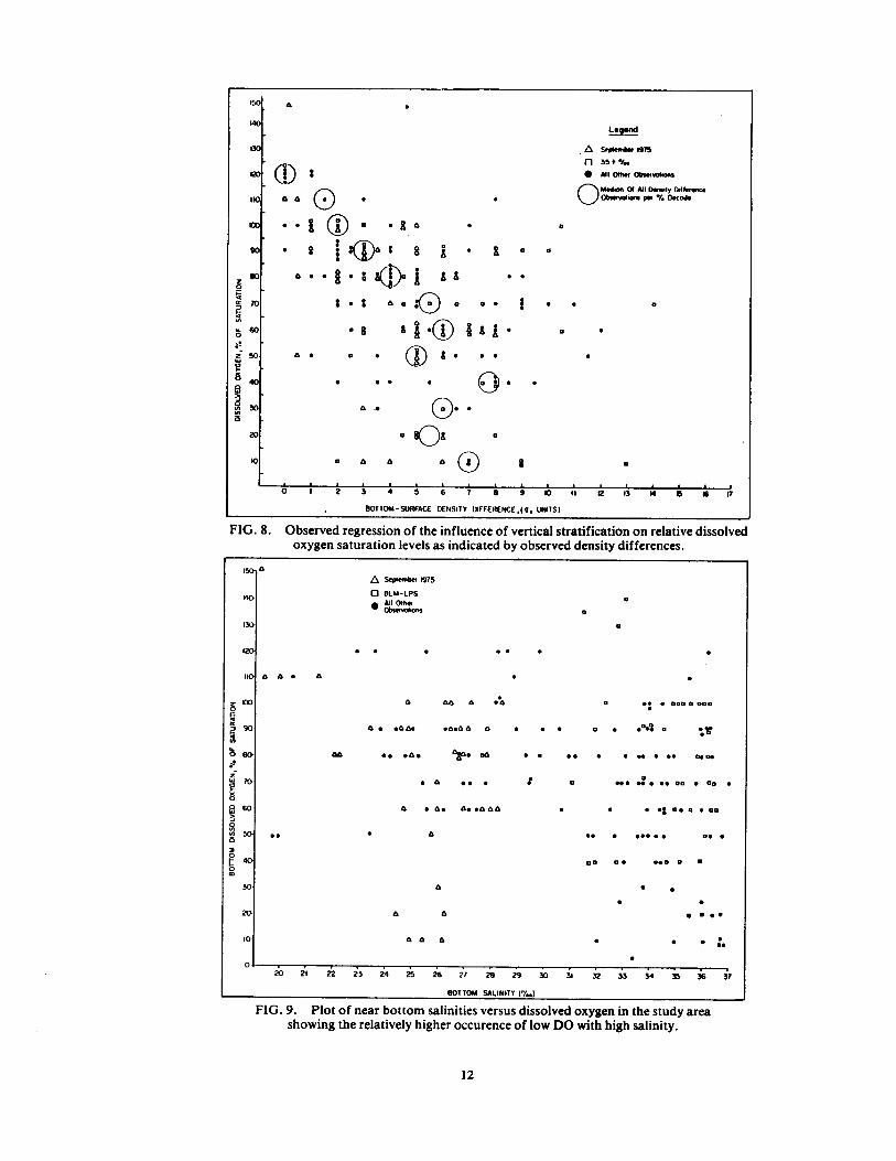
Cruise II, August/September, 1978 .. . . . . . . . . . . . . . . . . . . . . . . . . . . . . . . . . . . . . . . . . . . . . . . . . . . . . . . . . . . . . . . . . . . . . . . . . . . . . . . . . . . . . . . . . i l 8. Observed regression of the influence of vertical stratification on relative dissolved oxygen saturation levels

as indicated by observed density differences . . . . . . . . . . . . . . . . . . . . . . . . . . . . . . . . . . . . . . . . . . . . . . . . . . . . . . . . . . . . . . . . . . . . . . . . . . . . . ., . 12 9. Plot of near bottom salinities versus dissolved oxygen in the study area showing the relatively higher

occurrence of low DO with high salinity .. . . . . . . . . . . . . . . . . . . . . . . . . . . . . . . . . . . . . . . . . . . . . . . . . . . . . . . . . . . . . . . . . . . . . . . . . . . . . . . . . . . . 12 10. Plot of total percent light transmission with percent saturation of dissolved oxygen at various bottom

water depths (After Harvey, 1960).. . . . . . . . . . . . . . . . . . . . . . . . . . . . . . . . . . . . . . . . . . . . . . . . . . . . . . . . . . . . . . . . . . . . . . . . . . . . . . . . . . . . . . . . . . . 13 11 . Program organization chart . . . . . . . . . . . . . . . . . . . . . . . . . . . . . . . . . . . . . . . . . . . . . . . . . . . . . . . . . . . . . . . . . . . . . . . . . . . . . . . . . . . . . . . . . . . . . . . . . . ., 24 12. Maps of the study area-(Top) Location of study area; (Bottom) Study area showing sampling sites. . . . . . . . . 26 13 . Plot of actual sampling sites around a primary platform showing underwater obstructions . . . . . . . . . . . . . . . . . . . . . 31 14. Geographic representation of a range/range positioning mode and radar presentation of ship on location

when using variable range marker (VRM) positioning .. . . . . . . . . . . . . . . . . . . . . . . . . . . . . . . . . . . . . . . . . . . . . . . . . . . . . . . . . . . . . . . . . . 39

LIST OF TABLES

Table Page

1 . Monthly variation in surface and bottom density difference (% Frequency of occurrence by density differ-ence classes) .. . . . . . . . . . . . . . . . . . . . . . . . . . . . . . . . . . . . . . . . . . . . . . . . . . . . . . . . . . . . . . . . . . . . . . . . . . . . . . . . . . . . . . . . . . . . . . . . . . . . . . . . . . . . . . . . . . . . . . . 13

2 . Oil Spills Offshore Louisiana (1973-1977) . : . . . . . . . . . . . . . . . . . . . . . . . . . . . . . . . . . . . . . . . . . . . . . . . . . . . . . . . . . . . . . . . . . . . . ., . . . ., . . ., . 14 3 . Study platform identifying characteristics . . . . . . . . . . . . . . . . . . . . . . . . . . . . . . . . . . . . . . . . . . . . . . . . . . . . . . . . . . . ., . . . . . . . . . . . . . . . . . . . . . 27 4 . Master sampling scheme for each Primary Platform, Secondary Platform and Control Site . . . . . . . . . . . . . . . . . . . . 34 5 . Sample coding system . . . . . . . . . . . . . . . . . . . . . . . . . . . . . . . . . . . . . . . . . . . . . . . . . . . . . . . . . . . . . . . . . . . . . . . . . . . . . . . . . . . . . . . . . . . . . . . . . . . . . . . . . . . 41 6 . Study element codes by work group . . . . . . . . . . . . . . . . . . . . . . . . . . . . . . . . . . . . . . . . . . . . . . . . . . . . . . . . . . . . . . . . . . . . . . . . . . . . . . . . . . . . . . . . . . 42

ABSTRACT

Twenty-four sites on the continental shelf of the Louisiana coast have been studied for long-term cumulative ef-fects of petroleum production in the region of offshore platforms. Four primary study platforms and four control sites were visited in May, 1978, August/September, 1978 and January 1979. Sixteen secondary platforms were sampled Au-gust/September, 1978 . Sampling and analysis included hydrography and hydrocarbons of the water column ; sediment physical characterization, hydrocarbons, trace metals, and contamination with depth; and populations of the meia fauna, macroinfauna, macroepifauna, demersal fishes and species associated with the "artificial reef" brought about by the platform . Bottom studies extended from 100 to 2000 m away from platforms and were therefore indicative of regional as opposed to localized contamination. Sites were located from S km (3 mi) to 115 km (73 mi) from shore and extended from the west shore of the Mississippi Delta (89°32'V1) to a line south of Marsh Island (91 *44'W). Results confirm widespread, chronic contamination with hydrocarbons and metals with some apparent incorporation of pol-lutants into biota found at platforms. Over *the entire study area absolute amounts of contaminants vary widely show-ing a general concentration in the nearshore and eastern portions where the Mississippi River apparently contributes more contaminants than petroleum production platforms. Platforms vary widely in the types and amounts of pollut-ants traced to them . A distinctive pattern of expected contamination with platform operating type is not seen. Benthic populations are indicative of a stressed environment caused from high freshwater and sediment loading from the Mis-sissippi and periodic cyclonic storms . There are also localized platform influences on benthos in isolated cases. A few platforms are conclusively indicated as contributing to pollution in sediments up to a 2000-m distance .

Vii

I . HOW TO USE THIS REPORT

This report is divided into three volumes according to content : Volume I contains Principal Investigator results and data syntheses for pollutant fate and effects studies, Volume II contains results of the artificial reef studies, and Volume III is an executive summary .

The report organization and style have been set up according to accepted practices of scientific writing using the Style Manual for Biological Journals, second edition, American Institute of Biological Sciences, 1964 .

A. Volume I, Pollutant Fate and Effects Studies Volume I is separated into eight Parts, each of which

represents a Work Group or combination of closely sim-ilar Work Groups as set up under the program organiza-tion . Each of these Parts is written to stand alone in reporting significant findings and conclusions on a gen-eral subject concerning the impact of petroleum produc-tion platforms on the central Gulf of Mexico Outer Continental Shelf (OCS) . Therefore, a reader of the report with a special interest in trace metal contami-nants, for example, will go to Volume I, Part 4 where may be found the pertinent information on methodolo-gies, results and discussion . Since the background infor-mation and logistics of sampling around the platforms studied is the same for each discipline, that information is given in Part 1 and should be read prior to in depth review .

Volume I, Part 8 is a compilation of data from the complete data base assembled by the Data Manager and submitted as a requirement of the project as a data tape . Basic results have usually been manipulated or summa-rized prior to publication in Part 8 in order to present as brief a data inventory as possible while giving as much information as practicable for those with a need to use the results in criticism or better understanding of the conclusions reported . Therefore, in some instances, it is possible to go directly to Part 8 and get base data for use in comparative studies, while in other instances such as interpretation of gas chromatographic analyses a repro-duction of the complete chromatogram file would not be useful .

B. Volume II, Artificial Reef Studies Volume II, Artificial Reef Studies, is required by the

sponsor to be a separate part of this report . Otherwise this study area should be viewed as another of the seve-ral main study disciplines in that significant interaction between the biofouling research team and the rest of the group was achieved in data gathering, analysis and syn-thesis . As originally conceived those parts of the study reported in Volume I were to form a pollutant fate and effects study and the artificial reef work was to describe the added ecological potential of the hard substrate pro-vided by the platform . In practice, sampling and data synthesis required that the two research efforts be com-bined ; the results show that on the Louisiana OCS, plat-form biofouling organisms and associated fauna are a basic part of the regional ecology and indispensable to an understanding of the fate and effects of platform derived contaminants .

C. Volume III, The Executive Summary Volume III is a brief synthesis of all pertinent back-

ground information, project activities, and scientific conclusions in the form of a guidebook intended to give a quick understanding of the project to administrators, decision makers, conservation groups and scientists . It is an attempt to transcribe technical data into terms understood by the knowledgeable layman . Volume III has been prepared by the Program Manager from his understanding of each discipline and through consulta-tion with each Principal Investigator (PI) . In writing it he has transcribed PI conclusions without further inter-pretation ; however, he accepts responsibility for the content .

Though it is the final section of this report, Volume III, The Executive Summary, may be read prior to any other . The reader can become acquainted with back-ground information, scientific studies, results and con-clusions, and should interest lie in one or more of the various disciplines, a complete understanding may be gained in Volumes I and II .

II . INTRODUCTION TO PART 1

A. Philosophy of the Study It is important that the user of this report under-

stand the basic goals of the study and why the various tasks were designed as they were . The philosophy gov-erning the study was built around the need to determine the long-term effects of any petroleum production plat-form activities on a large area of possible influence. This is in contrast to studies which focus attention only during the drilling or production phases or on localized effects at particular structures . The Bureau of Land Management (BLM) used the premise that just the phys-ical presence of the platform and the fact that wells were drilled causes a disturbance in the immediate area . What has not been known previously is what cumulative effects hydrocarbons and metal contaminants may have produced at some distance from production facilities, over various platform lifespans, during production of different types of hydrocarbons, in various water depths and bottom conditions . From this type of information the decision makers can interpret how to improve OCS leasing techniques to mitigate possible effects in other potential production areas, design monitoring schemes for those areas, and design further research to yield more results useful in governing offshore operations .

In assessing long-term, cumulative effects it is not enough to know how much of a particular contaminant is present at any one sampling location . This informa-tion should be compared with amounts of materials found in benchmark studies of pristine areas or to levels which produce known ecological harm ; then statements about that particular substance may be postulated . However, in order to show ecological effects the data must be critically examined in concert with other param-eters . Thus a data synthesis effort using sophisticated mathematical manipulations of large data bases by com-puter techniques is essential . The sponsor has provided for this requirement in the establishment of particular data synthesis tasks .

This report is in response to a study protocol which was stringently set out in proposal requirements in the request for proposals (RFP) . Contract specifications took into account a diverse set of disciplines and inte-grated spacial and temporal analyses in a program which required close adherence to protocol by PI's, thus assuring PI response to stated goals .

B. ' Legislative Authority Behind the Study In 1953 the OCS Lands Act established Federal juris-

diction over the submerged lands of the OCS outside of state boundaries and charged the Secretary of the Inte-rior with responsibility for administration of mineral exploration and development . Later legislation and liti-gation established that this realm extended from 3 miles offshore (except in Texas and Florida where the limit is three leagues) to the practical limits of exploration at the edge of the OCS in about 200 m of water . Distance of leased blocks offshore has steadily increased with dril-ling depth capacity . The BLM was given responsibility for governing leasing of submerged lands and the Geo-logical Survey (USGS) responsibility for production .

Following passage of the National Environmental Policy Act (NEPA) of 1969 the BI.M implemented

decision-making procedures which incorporated con-cerns for environmental safety . The OCS Environmen-tal Studies Program is a result of those concerns . This continuing program aimed at achieving an understand-ing of the overall effects of offshore production has been a specific line item in the Federal Budget . Thus these studies on the fate and effects of contaminants from platforms and the artificial reef effect of the plat-forms themselves are an effort with the highest Federal priorities developed according to distinct BLM goals .

C. Objectives of the Study Two sets of relevant objectives as stated by the BLM

are pertinent to this study .

1 . Objectives of the BLM OCS Environmental Studies Program . The objectives of the BLM OCS Environmental

Studies Program were developed to govern OCS studies . These are :

" to provide information about the OCS envi-ronment that will enable the Department and the Bureau to make sound management deci-sions regarding the development of mineral resources on the Federal OCS;

" to acquire information which will enable BLM to answer questions about the impact of oil and gas exploration and development on the marine environment ;

" to establish a basis for prediction of impact of OCS oil and gas activities in frontier areas;

" to acquire impact data that may result in mod-ification of leasing regulations, operating reg-ulations, or OCS operating orders to permit more efficient resource recovery with maxi-mum environmental protection .

2. Objectives of the Central Gulf Platform Study. From the definition of overall program objec-

tives, information needs were categorized and research programs outlined in these areas : (1) benchmark, (2) reconnaissance or descriptive, (3) fate and effects and (4) predictive modeling . The present study is primarily in the fate and effects category and was formulated by the sponsor to "determine the transport and dispersal, as well as the biological, chemical, and physical altera-tion and final repository of contaminants related to OCS petroleum development as well as the chronic and acute effects such contaminants impose on marine ecosystems." The specific objectives of this effort as stated by the request for proposals were :

determination of the distribution and concen-tration of petroleum hydrocarbons, selected trace metals, and well-drilling related sub-stances in surficial sediments and tissues of commercially and/or ecologically important benthic and demersal species ; examination of the microbial hydrocarbon de-gradation and nutrient cycling processes and related nutrient chemistry in surficial sediments ;

comparison of benthic communities, with em-phasis on selected "indicators," in the imme-diate vicinity of platforms with those at con-trol sites ; examination of the distribution with depth in sediments of petroleum hydrocarbons, se-lected trace metals, and well-drilling related substances (i .e ., to provide some measure of persistence) ; investigation of the biofouling communities and "artificial reef" effect associated with se-lected platforms representing a variety of pro-duction types and durations .

D. Relationship to Previous Studies Most studies of the ecological effects of petroleum

in the ocean have come about as a result of disastrous spills . These reports have shown a wide range of effects depending on the spill magnitude, pollutant type, geo-graphical location, time of year and efforts to control the damage. The subject of large petroleum spills is quite controversial and is not the primary focus of this work . Evans and Rice in their 1974 review article state that knowledge of "the ecological effects of chronic sublethal oil pollution is essentially non-existent ." That statement still holds true with respect to OCS ecosystems . Chronic contamination from hydrocarbons and trace metals is the type examined in the study area and cumulative effects of this chronicity were investi-gated .

The most significant similar study was done in the Timbalier Bay area and the adjacent nearshore off Louisiana by Gulf Universities Research Consortium as the "Offshore Ecology Investigation" (OEI) . The re-cent reappraisal of the data gathered during that study (Bender et al ., 1979 ; Ward, Bender, and Reish, 1979) is particularly relevant to the findings of the present program . Conclusions from Bender et al . (1979) were these : (1) Timbalier Bay has not undergone significant

ecological changes as a result of petroleum operations ; (2) the overall region exhibits every indication of good ecological health ; (3) concentration of contaminant compounds are sufficiently low so as to present no bio-logical hazard ; and (4) the Mississippi River and associ-ated natural phenomena cause significantly greater envi-ronmental perturbation than petroleum operations . It was pointed out by Bender et al . (1979) that in retro-spect the design of the OEI might have been better and that subsequent results may have changed . These retro-spective criticisms fit well with the major goals of the present program in that more pertinent data are pro-vided for platforms studied in the OEI; subtle cumula-tive effects not thoroughly investigated are sought in this study, and even more data on the river influence are now at hand .

The continuing research directed by the National Marine Fisheries Service (NMFS) on the Buccaneer Oil Field (BOF) offshore Galveston, Texas, is providing in-formation which is quite complementary to the present work . A number of the PI's on the present study are also involved in the BOF work allowing for early access to data for extensive comparison . This has led to better understanding of results from both projects and, in turn, a more useful data synthesis .

Other BLM studies in the benchmark program have been used for comparison, especially the South Texas Outer Continental Shelf (STOCS) program and the Mis-sissippi, Alabama, Florida (MAFLA) program . The relationship to these studies is complementary in that the benchmark data are used for baseline or control in-formation when the control data from this study are not adequate . Since the MAFLA region is so different in ecology, it offers the chance for speculation about the types of ecological changes which might be forecast should petroleum production occur . Similar conceptual modeling will be possible on other OCS areas based on these findings, and research plans can be formulated to properly monitor development and production activities .

III. BACKGROUND INFORMATION ON THE LOUISIANA OCS

A. Physiography of the Louisiana OCS

1. Geology The Gulf Coast geosyncline, which extends

across the northwestern Gulf from about the middle of the East Coast of Mexico at the Taumalipas carbonate platform to the Florida carbonate platform at Cape San Blas, is the dominant structural element of the Louisi-ana OCS. This area of Cenozoic terrigenous sediments is nearly 20-km thick and extends from as much as 320 km inland to the Sigsbee Escarpment at the edge of the northern Gulf continental slope . The most significant source of these sediments from the early Tertiary until late Tertiary was the Rio Grande . Changes in climate which caused a gradual desertification of the western U.S . shifted major outflows to the Mississippi River, which remains the dominant sediment source to the Gulf . The gently sloping, relatively wide continental shelf has numerous topographical features representing relict shorelines, distributary ridges, coral reef remains and circular mounds associated with salt domes . These salt domes are diapiric intrusions from thick underlying deposits of the geosyncline and are the primary source of traps for petroleum in the central and northwestern Gulf . Much study of the geology of the Gulf geosyn-cline, and especially of the importance of the Louann salt beds, has been done during petroleum exploration . Still the origin of the Gulf of Mexico and its dominant physiographic features are as yet unresolved (Uchupi, 1975) . The aspects of Gulf geology important for this report are the recent history of the study area, how it re-lates to pollutant incorporation into the sediments and what potential for harmful effects may accrue .

Over the Central Gulf Platform Study (CGPS) area, surface and near-surface sediments are nearly ex-clusively derived from the Mississippi River . These are very fine fractions of silty clays and clayey silts with low sand content except in areas of accretion or shoals asso-ciated with distributary mouths and nearshore drift; for example, Ship Shoal area (Platform 19 of this study) is representative of one of these anomalous regions . The greater extent of the study area slopes gently to the edge of the OCS and is accruing sediments at a relatively rapid rate . Deposition from nepheloid layers and tur-bidity currents is speculated to account for the foreset bedding and extensive lamination seen . This rapid ac-cretion of unconsolidated materials leads to extensive slumping of the sediments with extensive mixing over time . This is referenced by numerous investigators and may be important for this study in explaining the rela-tive amounts of contaminants found in the sediments in this study (Bouma, 1972 ; Uchupi, 1975) . In the rela-tively rapid deposition of pediments over the Louisiana OCS in recent geologic times, significant diapirism has occurred in underlying finer elastics giving rise to nu-merous "mudlumps" over the area . These mudlumps, along with the larger, older intrusions from salt domes, provide the most prominent relief to the study area .

As far as is known the complete region of the study OCS is underlain by the Louann salt and hun-dreds of diapirs have provided the upthrusted traps for hydrocarbons . Many of these structures have not been

drilled . The wedge of salt in the Gulf geosyncline thick-ens toward the south and has moved slowly southward with the continuing deposition of its overburden . It ex-tends almost to the Sigsbee Escarpment, which demon-strates a dramatic dropoff to the deep oceanic base-ment . Diapirs and the potential for petroleum deposits are found on the deeper continental slope as well as the shelf . Depending on the economic and political condi-tions regulating petroleum exploration it is probable that further extensive exploration of the Louisiana shelf and slope will take place .

Studies in mineralogy of the region demonstrate the continued influence of the Mississippi River and the predominant types of clay minerals expected from the mid-continental United States . Montmorillonite (smec-tite) predominates and occurs up to ten times as abun-dantly as illite and kaolinite with some variation accord-ing to the technique used in X-ray diffraction analytical methods . The latter minerals are in about equal levels with illite sometimes slightly higher (McAllister, 1964) . During McAllister's study, which covered approxi-mately the eastern half of the present study area, he found no significant difference between diffractograms of samples ; he inferred from cores 300 to 334 cm long that the mineral topes and gross percentages have not changed in the time necessary to accrue such depth of deposits . This further indicates one set of depositional origins for many of the eastern stations during this study . Numerous studies have shown the several deposi-tional regimes of the Mississippi delta, and this informa-tion complements the findings for current sedimenta-tion extending from the present birdfoot delta . The problem with having knowledge of this sedimentation origin is that as yet we do not know the rates of accumu-lation . This is important because this study attempts to date hydrocarbon and trace metal contaminants as they may have accumulated during the history of petroleum production offshore Louisiana .

Mineralogy studies also indicate possible prob-lems with contaminant retention in study sediments be-cause of the clay types . The major types are of a 2 :1 lat-tice type having a moderate to high cation-exchange ca-pacity . This gives rise to an ability to "scavenge" ions from seawater anti thus concentrate certain materials significantly . The potential for adsorbing hydrocarbons just as the petrogenitors of present petroleum deposits were concentrated causes concern that similar concen-tration of contaminating hydrocarbons from man's ac-tivities may be significant .

2. Oceanography

a . Introduction The Louisiana OCS that constitutes the study

area is dominated by the Mississippi River . The magni-tude of the Mississippi's discharge, second only in the world to that of the Amazon River, causes it to affect water masses and circulation patterns for over 100 miles to the west ; with the addition of the discharge of its sa-tellite river, the Atchafalaya, its presence is discernible as far west as Galveston, Texas . The Mississippi River system also carries to the Gulf a very heavy sediment

load and a quantity of hydrocarbons that is greatly in excess of that from natural seeps or from production platforms . The Mississippi River's "birdfoot" delta, which extends almost to the edge of the continental shelf, effectively blocks shelf circulation inflows from east of the delta . These factors, when added to the strong meteorological processes at work in the area and the area's proximity to the ever shifting dividing line be-tween the complex eastern and western Gulf of Mexico oceanic circulation systems, result in a very complex oceanographic regime .

Unfortunately this shelf area has not received the attention of physical oceanographers that it deserves (or perhaps its very complexity has discouraged all but the bravest scientists) . The focus of research in the Gulf of Mexico has been in the waters off the shelf or on the Texas and MAFLA shelves . The result of this omission is that many of the oceanographic processes at work on the Louisiana shelf can only be implied (based upon the-oretical considerations) . Only a few of these processes have been directly observed or computed .

In the following sections some of the more significant oceanographic processes are discussed and observations of their occurrence presented . These in-clude estimates of advective flows, bay and shelf water exchanges, and mixing rates . The results of the oceano-graphic observations made on or simultaneously with the three Central Gulf Platform Study cruises are pre-sented, and seasonal variations in oceanographic condi-tions that have a pronounced effect upon the marine biological community are given .

Since hydrographic and physical obser-vations of the waters of the study area were not planned as a primary focus of attention, these results are not pre-sented in detail here because the data are not sufficient to develop definitive conclusions . Instead these data are put into perspective with, compared to and in some cases combined with results from other studies to de-velop a general description of the study area physical processes . This general discussion gives an indication of the fate of contaminants carried by the currents and riv-erine-born sediments and pollutants . Thus some expla-nations of physical influences on contaminant fate can be developed from synthesis of laboratory data from this project .

The data summary of hydrographic analyses is given in Volume I, Part 8 for more understanding of a particular station or season .

b. AdvectiveProcesses

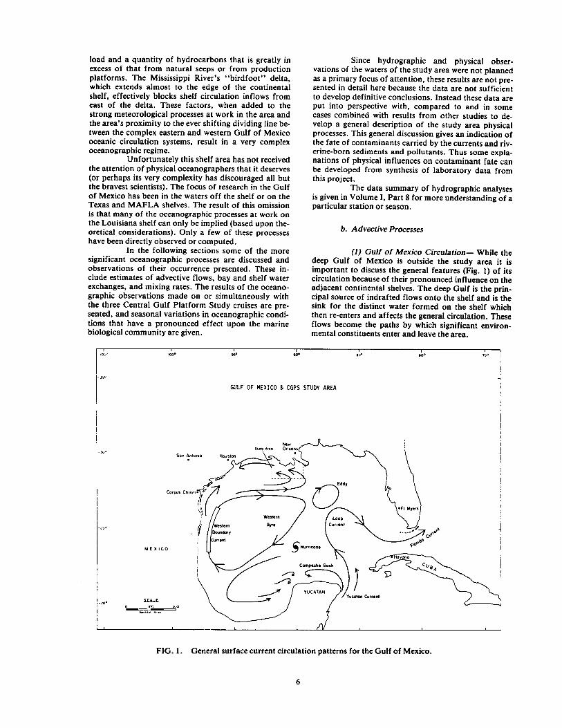
(1) Gulf of Mexico Circulation- While the deep Gulf of Mexico is outside the study area it is important to discuss the general features (Fig . 1) of its circulation because of their pronounced influence on the adjacent continental shelves . The deep Gulf is the prin-cipal source of indrafted flows onto the shelf and is the sink for the distinct water formed on the shelf which then re-enters and affects the general circulation . These flows become the paths by which significant environ-mental constituents enter and leave the area .

i0': i00. 91° 90' Ya° YO° lf° I

I

GULF OF MEXICO 6 CGPS STUDY AREA

San Aniomo Houston

Corpus Cnnsi, " 0 r~

MEXICO

SCALE

o K+n a.o

~Eddy

~/ BFI Myars

Western Loop Gyra Currant

,FHurricons \

Cornpeche Bank

YUCATAN

-I . . _ . . ~ GJtie0

I

Movono

CVB

D 4 I i Yucatan Current

FIG. 1 . General surface current circulation patterns for the Gulf of Mexico .

The principal deep water circulation fea-ture of the Gulf of Mexico is the Loop Current . Water enters through the Yucatan Strait as the Yucatan Cur-rent and flows in a clockwise loop which extends well up into the eastern Gulf and then exits via the Florida Strait as the Florida Current (Nowlin, 1972) . In winter and early spring the Loop Current extends to 27°N but by early summer the penetration can reach 29°N . In late summer the northern part of the Loop Current com-mences its development into an anti-cyclonic (clockwise) eddy . By late fall and early winter the eddy is fully sepa-rated and begins to move southwest . At that time the Loop Current has retreated and flows closely by Cuba (Ichiye, Kuo, and Carnes, 1973) . The extent of penetra-tion of the Loop Current can vary from year to year . Molinari (1978) reported that large summer-fall in-trusions occurred in 1966, 1969, 1973 and 1974 followed by maximum penetration in the winter rather than the summer.

The deep sea exchanges between the eastern and western Gulf are still not understood and there is little data to define the deep circulation of the Gulf and its interchange with the Yucatan Current (Nowlin, 1972 ; Molinari, 1978) . The relative homogene-ity of the waters of the western Gulf and the low geos-trophic gradients suggest that there is no massive ex-change .

The general winter circulation in the western Gulf consists of a clockwise gyre, having a broad westward flow for its southern limb, a narrow east-northeastward flow for its northern limb and flanked to the north by a west-southwestward current along the outer Texas-Louisiana shelf . The general sum-mer circulation in the western Gulf is much more com-plicated and variable with numerous small cyclonic and anti-cyclonic gyres (Nowlin, 1972) . This circulation is principally wind driven . Blaha and Sturges (1978) have found that seasonal variation of western Gulf currents is consistent with the sea level response to wind stress . They even suggest the occurrence of a western boundary current in the Gulf similar to the Gulf Stream or Kuro-shio (Sturges and Blaha, 1976) .

(2) Louisiana Shelf Circulation- The prox-imity of the Louisiana OCS to both the eastern and western Gulf circulation systems makes it difficult to de-fine which system is the source of the offshore waters that are advected onto the shelf west of the Mississippi Delta . Whether the source for these waters is the west-ern gyre or eastern Loop Current and eddy has not been determined . From an analysis of drift bottle recoveries Temple and Martin (1979) show an offshore eastward circulation for March and April of 1962 which would suggest the western gyre as the source; dynamic compu-tations by Ichiye (1960), which show a northward flow-ing current just south of the Mississippi Delta in July of 1954, suggest the eastern Loop Current or eddy as the source . These differences are consistent with the sea-sonal growth of the eastern Loop Current system dis-cussed earlier (Ichiye et al ., 1973) . Due to the variability of the Loop Current system from year to year this sea-sonal change in the source of the shelf water may also vary, and for much of the year there may be a complex mixture of waters from the two systems present . While both the eastern and western Gulf waters have the same

origin in the central Carribean Sea, the western waters have been modified by warming, particularly while flowing over Campeche Bank north of Yucatan, and by net evaporation (Franceschini, 1961) . Oceanographic features of the shelf circulation (Fig . 2) are discussed in the following sections .

The current regimes on the Louisiana shelf have been described by Temple and Martin (1979) using drift bottle recovery data from 1962 and 1963 and by Oetking et al. (1974a) using current meter data from 1972 and 1974 . The best discussion of currents and cir-culation is to be found in Murray (1976) . Seasonal vari-ations in currents are as follows :

" January-February-in western Louisi-ana currents were westerly and offshore with velocities ranging from 9-14 km/day ; most of the flow just west of the' Delta was to the north and onshore with velocities of 5 km/day.

" March-May-similar to January-Febru-ary but with velocities ranging from 7-14 km/day in the west and 1-3 km/day just west of the Delta .

" June-July-reversing their earlier west-ward and offshore directions, currents were to the north and east . The north-erly currents were generally restricted to nearshore waters and the eastward movement restricted to the deeper wa-ters over the shelf . Onshore velocities ranged from 1 to 9 km/day with an aver-age of 3 km/day.

" August-currents shifted to onshore to the northwest but velocities had slowed to a rate of 2-3 km/day .

" September-December-currents returned to a generally westward offshore flow similar to January-February with an av-erage velocity of 5 km/day.

A significant feature of the circulation on the Louisiana shelf is the persistence of a northward flowing current o1' offshore waters just west of the Delta which loops around to the west and offshore . This northward flow of drift bottles persisted from February through May. Ichiye (1960) indicates such a loop current occurring in July 1954, as shown in the density difference distribution plot in Fig . 3 . The occurrence of closed gradient contours in the salinity distribution shown in Fig . 4 indicates the occurrence of upwelling of subsurface offshore waters . Figure 5 shows the surface density distribution observed in Cruise II in August/September, 1978 . There is a similar loop current indicated but it is further to the east . The pres-ence of this loop current suggests that the Mississippi River discharge, except for some partial mixing upon debouching from Southwest Pass, undergoes little further mixing until it is west of Barataria Bay . Its pres-ence also suggests the persistence of unmixed offshore waters well inshore west of the Delta . The presence of Mississippi and Atchafalaya River waters in the shelf circulation is discernible as far west as the longitude of Galveston where salinities again approach 35 °/00 (Nowlin, 1972) .

.... ~Z-

J _ ~° ~ .o~c., nn nr w .w

.... .

. .,ti,, l NV ~? ""t

V 7 , M, ~.L_

t, ~ dE

#61 Inertial Upwalling

i ShlH Westward D^" . . ~ . ~` y a...nt . .

" ,"

.21

Winter Shelf Water Fomnalion / / Offshore IIIdfO}f

" S'u., SOES Nom' ~~

FIG. 2. General pattern of surface circulation in the study area of the Louisiana OCS.

I . . . . -

U~, IN.

DENSITY GRADIENT la%) - .0

S

=SAInf-C- S4-9

&NN

MAL

FIGA . Density difference between surface waters and 10-m depths from combined Central Gulf Platform Study data and Ichiye (1960) .

8

~n~ Cw 4wi+~ 7p 1 N~ ~1G~LY C~tt

wax.

~_ .o.r~T ,, 4~°i : :/'ply ~ .

.. ; . . ,~ .

p. .. -- ~

.

s _u- .- . . . . . . .

!)

11~

SALINITY (y�)

IAK~A C,- 54-9

S.ai Sww~p S~w~

~y i / cYt b

FIG. 4. Surface salinity measurements in the study area is 1954 indicating apparent upwelling of high salinity offshore waters in the West Delta area (Ichiye, 1960).

... w ae": " . r. ~- v ,+ :iwc .~ n. . ~x ,\

'~ f p .ow. d

(/ .+

w~u~

\\ INA

4P Is ~- O

__ . . ~

.

/^l

" \ ' - . . .

. _,

20

~'~p .. . . . . - "NONUILY Of DENSITY I .,) . . . . . . . ~ . 10-11.1000

" STUDY SITES

e!r r O YJ W

FIG. S. Surface density as drawn from Cruise II data, August/September, 1978 .

9

(3) Dissolved Oxygen in the Waters of the " Stratification . Due to the influx of low- Study Area-On Cruise I in May 1978 the occurrence of density Mississippi River water into the bottom dissolved oxygen (D.O.) levels of 3 ppm or less area and the seasonal warming of sur- were observed at half of the sampling sites with levels face waters, intense vertical-density stra- around 1 .5 ppm observed at two sites. Sampling design tification frequently occurs . Stratifica- provided for D.O . sampling at 1 m below the surface lion inhibits vertical mixing and de- and at 10-m intervals until reaching less than 10 m from creases the movement of oxygen rich the bottom ; therefore, near bottom samples were not al- surface waters downward. When this ways taken. Because of this, data do not adequately de- stratification occurs, existing deep D.O . pict the low D .O . levels actually present . The persistence levels are depleted due to the oxidation and extent of the near-anoxic and anoxic conditions was of organic detritus and to oxygen uptake confirmed by the very poor bottom trawl collections as by bottom and near bottom biota . In well as the observance of numerous recently dead orga- Fig. 8 the influence of vertical stratifica- nisms . On Cruise I, Platforms 1 and 2 and Controls 21 lion upon the relative D.O . saturation and 22 were affected and on Cruise II a number of near- levels is indicated by the medians of the shore sites were affected as shown in Figs. 6 and 7. Fig- observed density differences . ure 6 gives results of analysis for D.O . taken in the " Low D. 0 . Offshore Subsurface Waters. water sample nearest bottom and Fig . 7 shows compara- As discussed earlier, there is a persistent ble results from observations of emigration of demersal indraft into the study area of offshore nekton and poor condition or death of numerous infau- subsurface waters that are low in D.D . nal forms caught in trawls . These data are more com- Waters at 200-m depths offshore which pletely given in Volume I, Part 8 . typically might have salinities of 36 ppt

This low D.O . phenomenon has been re- and D.O. levels of 2.6 ppm (30% rela- ported in the literature since at least the mid-thirties five saturation) are upwelled and ad- (Conseil Perm. International pour ('Exploration de la vetted inshore . These levels are fre- Mer, 1936) and has been "rediscovered" in the liters- quently further depleted due to the same ture several times . Richards (1954) mentions the gener- processes caused by stratification . Fig- ally low D.O . found in the areas of the Gulf under the ure 9 shows the frequent occurrence of influence of high organic sediment loading . Others have low bottom D.O .'s at salinities higher discussed the occurrence (Richards and Redfield, 1954 ; than 35 ppt which are attributable to this Oetking et al ., 1974a ; Ragan, Harris and Green, 1978) . influx of low D.O . offshore subsurface Gunter (1952) discussed at length the changes in sedi- water. This water then mixes with lower mentation patterns of Mississippi River runoff due to salinity shelfwaters which usually have the leveeing of the river in the last 100 years . He shows higher D.O, levels . Ragan et al . (1978) that whereas formerly most sediments were deposited attribute the low D.O.'s observed in on the broad river plain, marshes and shallow bays dur- September 1975 to stratification and ing floods, they are now funneled directly into the Gulf abeyance of wind-induced mixing . A down swiftly flowing leveed flumes . It is likely that this similar condition occurred in 1978 but has induced a broader and more pronounced lowering with the passage of tropical storm Debra of the bottom oxygen by introducing more smothering through the area, 27-29 August, intense silt into the OCS and in slugs of floodwaters as opposed mixing and oxygen replenishment re- to the long-term slow runoff of recent geologic times . suited .

From observations made by Nicholls " Photosynthesis . Ragan et al . (1978) State University, Ragan et al . (1978) reported the wide- point out that in addition to the atmo- spread occurrence of oxygen deficient bottom waters sphere, photosynthesis is an important (<2 ppm) . The low D.O . condition was first observed in source of D.O . in surface water . The May of 1973, particularly within the depth range of depth to which this process is significant 6-33 m. This condition persisted from May 1973 to is difficult to assess for the study area March 1974 and ranged from 27% of the bottom being because some areas were observed dur- affected in December to 93% in July with an average of ing sampling to be extremely productive 52% . Over half of these affected waters were anoxic based on water color. In discussing pho- (0.0 ppm) . A subsequent study from May 1974 through tosynthesis, Harvey (1960) observed that August of 1975 showed a reduced affected area of only for light fluxes with a daily overage of 39% of which only 1/3 was anoxic . A more extensive 0.03 cal/square centimeter per minute or study program from September 1975 through August less, oxygen production is proportional 1976 shows a further decrease in the affected waters but to light energy . For fluxes greater than with no anoxic waters . They attribute the decrease in the 0.03 cal/square centimeter per minute affected areas to a decline in the volume of the Missis-

~ production is saturated or even de-

sippi River discharge. creases . An analysis of the transmissiv- The mechanisms which control bottom ity observations made at the surface and

and near bottom D.O. levels are many and complex. An at 10-m intervals and shown in Fig. 10 analysis of the observations reported by Ragan et al . suggests the occurrence of such pro- (1978) for 1975 and 1976 and of observations made on cesses . The bounding of the relative the three Cruises indicates that these levels are con- D.O.'s below 80% by the highest total trolled by three dominant processes, all of which may transmissivity indicates the limiting occur at the same time . effect of light levels and the saturation

10

M~Gw Yr~r ~pp~~ C-

D

xr IfO ~ '70.J

.h ,

11r~~ ~ j

~pw e

S ,o~o~w yc.oa. ,~~

rw i ~ ~t (/ ~ H~CI

~. \ . S ~ ~~. .

. . .~ . . .

._ b ,

71f w ' to 3

.C .- . . . . . . . . . . .-- . . . . . ., DISSOLVED OYYGEN ~ppn :

9 STUDY SITES p..

vuL

O q f0 7D ~0

FIG. 6. Near bottom dissolved oxygen levels taken during Cruise II, August/September, 1978 . .. . , ~.. .w . ..

40L0[+

S,~ . L

I~,~(' 1' J

N+~i N, . . ~ . . A

.." / . .~ . "" . . f z.

s . '

M N Sf

DEAD BOTTOM AREAS

6 STUDY SITES

75C&

"~

E

A b

h 1G . 7 . Areas with dead bottoms as evidenced by trawl catches and hydrographic data taken at platforms during Cruise II, August/September, 1978 .

11

0

CJ Ib O O O

~ ~ g a e ~ g C ~ o 100

90 ~ Q = j/ A BC t g °E ~ g o d ~ III/

i ogo e . .$ "" ~a~°~ as . .

s . : oo ;O o o . ~ . . 70

a .e e~ "O ~a~ " e

50

. . ~ . 40

o . O. . 30 a

ZO o ~/ to o

b a O D O Oj

0 1 2 3 4 5 6 7 B 9 10 11

BOTTOM-SURFACE DENSITY pFFERENCE,(O, UNITS)

Legend

A S,~ 1975 n 35+%. III All Oth . Obwwalwts

0 Mqdw% 01 All 0" . It 0,414, Obwvd~ pt, %'Docode

0

0

M 4 R n

FIG. 8. Observed regression of the influence of vertical stratification on relative dissolved oxygen saturation levels as indicated by observed density differences .

0 D Sea-en gas Q BlM-LPS " All qlKi

Obwwl~ o

0

120

II O O ~ O

= pp A Cp o A a ~~ ~ o00 0 ooa O F

90

90~ 66 6" "6 " ". Woe

7. W 70

I

I

" D "" N" N " "" 00 . 00

~ I ~ 60 C " o" ~" "CGG " " " "= O. O . 00 I J p

N

O "

O 40 Do 00 ..CI

0 m

JO O

20 O D o e of

to D o N

O 20 21 n 23 29 n 26 77 26 29 30 31 32 33 34 36 35 3l

BOTTOM SALINITY ("/w)

FIG . 9 . Plot of near bottom salinities versus dissolved oxygen in the study area showing the relatively higher occurence of low DO with high salinity .

12

photosynthesis . Total percent transmis-sivity is the product of the 10-m intervals and surface transmissivity measure-ments . Since the effect of photosynthe-sis on deeper D.O . levels is at best specu-lative, no further reduction of transmis-sivity measurements has been made .

FIG. 10. Plot of total percent light transmission with percent saturation of dissolved oxygen at various bot-

tom water depths. (After Harvey, 1960)

of higher light levels at the surface. The supersaturated observations shown in this figure may also be attributable to

Since bottom D.O . measurements are quite limited both in their number and duration it is dif-ficult to define the long-term monthly or even seasonal variation in their levels . However, since stratification is the principal controlling mechanism, and since the inflow of high-salinity offshore waters frequently enhances this stratification, the seasonal variation in the differences in density between surface and bottom waters can be used as an indication of probable bottom D.O . levels . When there is intense stratification in the summer or early tall it is likely there will be low DO's on the bottom . Table 1 shows the frequency of seasonal variations in surface-bottom density differences for the years 1963-65 (Temple, Harrington, and Martin, 1977), 1975-76 (Ragan et al ., 1978) and May 1978 to January 1979 (BLM-CGPS) .

(4) Estimate of Petroleum Hydrocarbons in the Mississippi River Discharge-The Mississippi River has an average discharge rate of 620,000 cfs (17,600 m3/sec) which is approximately 1 .5% of the world river runoff (Murisawa, 1968) . The world wide input rate of petroleum hydrocarbons into the oceans from river runoff is 1 .5 x 106 tonnes/yr (1 .6 X 106 m3/yr) (National Academy of Sciences, 1975) . The Mississippi's directly proportionate share of this input is then 24,000+ m3/yr (760 X 10-6 m3/sec) . This amount of hydrocarbon would result in a concentration of 45 ppb for an average river

TABLE 1 . Monthly variation in surface and bottom density difference (% Frequency of occurrence by density difference classes)

Bracketed Values : 6-17 meter depths Unbracketed Values : 18-92 meter depths

0 0 0 0 14 0 0 0 0 0 0 0 I 10.18 (0) (l2) (0) (20) (0) (0) (0) (0) (0) (0) (0) (0) (2)

:3 0 0 18 12 86 87 38 0 0 0 0 0 20 3-9 o (0) (0) (46) (20) (33) (43) (0) (0) (0) (0) (0) (11) (13)

100 100 82 88 0 13 62 100 100 100 100 100 79 ,°, a3 .. (100) (88) (54) (60) (67) (57) (100) (100) (100) (100) (100) (89) (85)

Mar . Apr. May June July Aug . Sept . Oct . Nov . Dec . Jan . Feb. Year A

Western Sect ion Sites 2-4, 10.12, 14-20, 22-24

63 48 50 56 8 13 0 0 0 0 0 0 20 I0-18 (25) (30) (0) (0) (0) (0) (0) (0) (0) (0) (0) (0) (5)

12 40 20 44 92 78 62 II 65 0 11 42 40 6 3-9 o (23) (30) (33) (0) (75) (43) (0) (0) (25) (0) (0) (20) (21)

a° p 25 13 30 0 0 9 38 89 35 100 89 58 40 0-3 (SO) (40) (67) (100) (25) (57) (100) (100) (75) (100) (100) (80) (74)

Mar. Apr. May June July Aug. Sept . Oct. Nov. Dec. Jan. Feb. Year

Eastern Section Sites 1, 5-9,13, 21

13

discharge of 17,000 m3/sec . Because of the industriali-zation of the U .S . it is reasonable to assume that this pollutant load is actually much higher .

Information on oil and grease from the EPA STORET Data Bank for Venice, Louisiana, just above the mouth of the river, is reported only to the nearest 100 ppb . At that level, all observations obtained in 1978 were reported as 0.0 mg/I . A concentration of 45 ppb would then be reported as 0.0 mg/I . Thus, this con-centration is not in conflict with the reported obser-vations . Given the magnitude of the Mississippi River discharge it would be beneficial to have oil and grease observed and recorded to a greater accuracy :

When the quantity of 24,000 m3/yr is compared with the quantity of oil spilled offshore, according to current U.S . Coast Guard data as shown in Table 2 , it is apparent that the hydrocarbons discharged by the Mississippi may be the dominant source of hy-drocarbons in the study area . This is probably partic-ularly true for the heavier hydrocarbon fractions .

B. Petroleum and the Louisiana OCS

1. Historical Background of the Offshore Oil In-dustry in the Gulf of Mexico Although offshore oil exploration is about ten

times more costly than onshore exploration, the increas-ing activities offshore in the Gulf of Mexico are appar-ently due to a decreasing reserve-to-production ratio

and declining exploration activities onshore . The first oil well drilled (March 1938) in the open water of the Gulf was in the area which became known as the Creole field, about 2.4 km from the coastline of Louisiana. Significant development to explore the offshore hydrocarbon deposits, however, did not commence until November 1947 when the Ship Shoal Block 32 field was found about 19 km from the Louisiana coastline . And not until the ownership and jurisdiction of the nat-ural resources of the seabed of the OCS had been de-fined by the Submerged Lands Act in May 1953 and the Outer Continental Shelf Lands Act in August 1953 did the leasing and development activities in the Gulf of Mexico accelerate . Since then, petroleum industry capi-tal has been attracted to offshore areas due to several factors . Among the more important ones are the discov-ery of sizable fields ; the higher success ratio for explora-tory wells drilled (26°Io success for offshore compared to 18% success for onshore) ; the more reserves found ; the larger size of the tracts being offered ; and the obtaining of acreage from a single owner (Weaver, Jirik and Pierce, 1969) . After the 1973 oil embargo, in response to calls for "energy self-sufficiency," the Department of the Interior expanded its OCS oil and gas leasing program . At the end of 1975, approximately 65 mobile drilling units were operating in the Gulf in water depths as great as 525 m and over 220 km from shore (Danen-berger, 1976 ; Harris, Piper and McFarlane, 1976) . By 1979 development had increased the number of

TABLE 2. Oil Spills Offshore Louisiana' (1973-1977)

Annual Spills Origin of Spill

Production Transportation Unknown Total Annual Spill Estimated Estimated Estimated Estimated

Year Number Quantity m3) Number Quantity (m3) Number Quantity (m3) Number Quantity (m 1973 2 0.2 - - 2 0.1 4 0.3

1974 17 1 .6 1 nil 6 0.1 24 1 .7

1975 94 4.8 9 0.2 60 1 .8 163 6.8

1976 490 237.0 7 19 .0 223 119.0 720 375 .0

1977 368 81 .0 2 1 .0 153 4.5 523 86 .5

Number of Spills in 1977

Quantity of - Origin of Spill Total by

18

250

70

7

17

ranspOrtahon Unknown 138

10

2

1

I

1

157

261

72

8

19

2

5

Unknown

0-0.034

0.034-0.18

0.18-0.38

0.38-1 .9

1 .9-3.8

3.8-19 .0

19+

Total by Origin

"89°30' to 91 °50' West Longitude.

5

368 3

14

153 524

platforms in the Gulf to 3342 (Jackson, 1979) . At pre-sent the Cognac platform at 300-m depth has proven the capability of production at significantly greater depths than previously attempted . Subsea production systems, deepwater guyed towers designed to yield slightly to en-vironmental forces, and other prototype equipment that are now being tested in the Gulf will greatly increase the capacity for offshore development .

The offshore areas along the Gulf of Mexico contain a substantial proportion of the United States pe-troleum resources and this is reflected by the extensive drilling activities in the last 30 years . In 1955., there were approximately 400 wells drilled offshore and the total footage was about 1 .1-million meters . By 1966, more than 1160 wells had been drilled with approximately 3 .2-million meters in total footage . Information for 1978 (Jackson, 1979) shows that of the 23,305 total wells drilled in the U .S . offshore, 83% or 19,390 have been drilled in the Gulf of Mexico . At the end of the year 99% of the producing U.S . offshore platforms had been developed in the Gulf of Mexico .

The rich oil and gas reserves, the increasing demand for energy, plus the desire for low-sulfur con-tent natural gases and crude oils from this area, espe-cially in heavily populated areas, make the Gulf of Mex-ico one of the most productive areas in the world in terms of quantities of oil and gas produced . The crude oil and condensate production in the Gulf accounted for 0.68% of the total domestic production of the United States in 1954 . In 1966, Gulf production was 8 .06% of the total domestic production . During this period, the Gulf production accounted for 30% of the increase in total domestic production (Weaver et al ., 1969) . In 1967, the average oil production rate from offshore completions in the Gulf of Mexico was about 150 bar-rels-per-day while the average for the total United States was about 15 bpd (Weaver et al ., 1969) . The offshore crude oil reserves in this area by December 31, 1967 were estimated by the American Petroleum Institute to be 2,374,576,000 barrels, which constituted approxi-mately 8% of the total United States crude oil reserves (Weaver et al ., 1969) . The annual oil and condensate production was about 336-million barrels in 1970 and about 389-million barrels in 1972 (Harris et al ., 1976 .) Although the production has shown a declining trend since 1972, as reflected by the annual production of 315-million barrels in 1975, from 1971 to 1975 about 1 .811-billion barrels of oil and condensate were produced from federal lands in the Gulf of Mexico, accounting for more than 10% of the nation's domestic crude oil production (Danenberger, 1976 ; Harris et al ., 1976) . It is estimated that by 1985, 14.5% of the anticipated do-mestic 23 .5-million barrel-per-day crude oil demand and 33.4% of the domestic gas demand will be supplied by the Gulf of Mexico production (U.S . Army Corps of Engineers, 1973) .

2. Historical Background of the Oil Industry Off Louisiana The most successful oil and gas exploration and

production in the Gulf of Mexico has been in the Louisi-ana OCS. The depositional history of this area has made it one of the most productive areas not only in the Gulf but in the hemisphere as well . In 1955, there were 50 off-shore fields cumulatively containing more than 400 pro-ducing wells which produced 0.1 07o of the total United

States domestic crude oil production (U.S . Army Corps of Engineers, 1973) . By 1967, there were 147 oilfields or gasfields off Louisiana . The 1967 annual production was 219-million barrels of oil and condensate, and 1-bil-lion Mcf of gas (Harris et al ., 1976), which represented 99% of the Gulf production that year . There were 14 giant fields off Louisiana in January 1968 and each had an ultimate recovery of at least 100-million barrels of crude oil (Weaver et al ., 1969) . From 1953 to 1975 more than 26-billion Mcf of gas and close to 3.8-billion bar-rels of oil and condensate were produced (Harris et al ., 1976) . Between inception of the OCS leasing program in 1953 and 1973, there were some 1800 offshore structures set up in offshore Louisiana waters from which more than 8800 exploratory holes have been drilled resulting in more than 510) producing wells ; production from these represents about 48% of oil and condensate and about 69% of the total United States offshore produc-tion under both Federal and State leases (U.S . Army Corps of Engineers, 1973) . The latest available informa-tion (Jackson, 1979) indicates the total number of struc-tures offshore Louisiana is now over 3100, about 93% of the Gulf total .

3. Economic Impact of the Oil Industry Oft Louisiana The oil produced off Louisiana provides reve-

nues to the federal government and the State of Louisi-ana as well as jobs in oil exploration, drilling and oil-re-lated refining and :manufacturing activities . The oil and condensate from the OCS off Louisiana had a produc-tion value of $3.5 million in 1953, with a royalty value of $0.7 million . These figures increased dramatically with the intensive development of the OCS. From 1953 to 1975, the cumulative production value was $15 .2 bil-lion, and the cumulative royalty value was $2.62 billion (Harris et al ., 1976) . Natural gas had a similar geometric growth from a production value of $0.25 million in 1953 to $1 .17 billion in 1975 . The cumulative gas production value from 1953 to 1975 was close to $6 billion with a cumulative royalty value of $941 million (Harris et al ., 1976) . All the products (oil and condensate, gas, gaso-line, liquid petroleum gas, sulphur, and salt) produced from the OCS off Louisiana from 1953 to 1975 had a cumulative production value of $22.4 billion and a cu-mulative royalty value of $3 .67 billion (Harris et al ., 1976) . Including the coastal parishes of Louisiana, there are some 8000 producing wells that contribute an annual payroll of about $150 million to the area (U.S . Army Corps of Engineer ., 1973) .

4. Important Ecological Impacts of the Oil Industry Off Louisiana The most significant ecological impact offshore

drilling activities have on the marine environment is the oil spilled either by accident or by normal operation . It has been estimated that at least 10,000 oil spill incidents occur each year 'throughout the world (U.S . Army Corps of Engineer's, 1972) . According to Melvin, Eh-renspeck, and Nordin (1977), the United States National Oceanic and Atmospheric Administration estimated that oil from natural seeps underlying the world's oceans entered the marine environment at a rate of more than 0.5-million tans per year, and offshore petroleum production added another 1 .1-million tons per year . The National Academy of Sciences (1973) estimated

15

that amount to be 87,500 tons per year, or 1 .3% of ail marine oil pollution . Considering that the concentration of production offshore Louisiana is the highest in the world it is reasonable to assume that a significant por-tion of this pollution is occurring on the Louisiana OCS.

Most production-platform spills involve failures in the sump system, the separator system or other hy-drocarbon-handling equipment . It was estimated in 1971 that a typical offshore well had an effluent rate of 2500 barrels of oily water per day ; with oil present at about 1000 ppm, this represents 2-5 bpd from each pro-ducing well (Alpine Geophysical Associates, Inc ., 1971) . This level of pollution has been cut dramatically over the past several years and normal produced water sepa-rators only permit 0-50 ppm of oil in the discharge .

a . Oil Spills on the Louisiana OCS Several spectacular oil spills in the last few

years captured widespread public attention ; two of these, the Exxon pipeline break and the Shell blowout and fire, occurred within the study area of this project . The pipeline break released an estimated 160,000 barrels of crude in the West Delta area in 1967 . The Shell spill started December 1, 1970 and lasted until April 16, 1971 . The location of this spill was approximately 7 miles south of Timbalier Bay . It was monitored by a va-riety of federal, state, and private agencies . At least two reports were published on it (Texas Instruments, 1971 ; Resources Technology Corporation, 1972) . Estimates of the total volume of oil spilled at and about the Shell platform ranged from 25,000 barrels, made by Shell Oil Company, to a 53,000 barrel estimate by the United States Geological Survey, and finally to a 90,000-119,-000 barrel estimate by the United States Environmental Protection Agency (Stone, 1972) . Another spill which received significant public attention was the Chevron Main Pass accident of 1970 . The spill was monitored by a variety of federal, state and private agencies . At least two reports were published (Murray, Smith and Sonu, 1970 ; Alpine Geophysical Associates, Inc ., 1971) . The United States Geological Survey estimated that the total volume of oil spilled at and about the Chevron platform was 30,500 barrels (Stone, 1972) .

There have also been numerous smaller spills throughout the years of extensive oil exploration and production in the Gulf of Mexico . Since 1964, there have been at least ten recorded spills greater than 1000 barrels that are directly or indirectly attributable to off-shore drilling and production operations (U .S . Army Corps of Engineers, 1973) . Many spills went unreported and the statistics of spills were by no means complete until issuance of OCS Order No. 7 by the United States Geological Survey in August, 1969, which required that all spills, regardless of size, be reported to the USGS. Is-sued by the same agency, OCS Order No . 8, which out-lined platform safety and pollution control require-ments, effective on October 30, 1970, and OCS Order No. 9, effective in early 1971, were, when combined with industry's own effort, very effective in reducing the number of spills in the Gulf of Mexico . From January 1, 1971 to December 31, 1975, 5857 spill incidents were re-corded with a total spillage of 51,421 barrels . The pro-duction during that period was 35,219 barrels per barrel spilled, which gave a spillage rate of 0.0028% . In fact, 85 .5% of the total spill volume was contributed by five

incidents . A single incident - the Bonita pipeline break in April 1974 - accounted for 38.6% of the total volume . Four of the five spills which exceeded 1,000 barrels were related to transportation of oil from OCS production facilities . Furthermore, 99.5% of the spills were smaller than SO-barrel spills, and accounted for 9.4% of the total spillage volume . Of the 20 spills of more than 50 barrels, nine were transportation incidents and six were caused by failures in production-platform equipment . No spills of more than SO barrels resulted from drilling operations including exploratory drilling although 4105 new wells were started (Danenberger, 1976) . Although the number of less-than-50-barrel-spill incidents in-creased, the amount of oil discharged decreased by more than half between 1971 and 1975 . The decrease in spillage was due to the preventive measures taken by the industry, the advance in technology with improved sump-system designs and better high-low-level controls, and the increase in enforcement of rules and regulations to prevent spills .

Since the enactment of the Water Quality Im-provement Act of 1970, considerable progress has been made in contingency planning and spill response . Of the estimated 10,000 oil spills which occur annually, actions have been taken in the majority of the cases to remove the spilled oil from the environment . Fast cleanup re-sponse to spills with trained crews and modern equip-ment also help to reduce environmental damages to a minimum . Apparently no significant mortality of ma-rine life resulted from the Chevron and Shell spills (Murray et al ., 1970 ; Alpine Geophysical Associates, Inc ., 1971 ; Texas Instruments, 1971 ; Resources Tech-nology Corporation, 1972) . The only environmental damage recorded as a result of the five largest spills be-tween 1971 and 1975 occurred when minor amounts of oil intermittently reached approximately 1000 feet of beach on the Chandeleur Islands after the September 9, 1974 Cobia pipeline break (Danenberger, 1976) .

Although a large spill receives more atten-tion, the more numerous, frequently occurring minor spills and natural seepage will have more important long-term ecological impact . The effects on the bios-phere of long-term sublethal intoxications and the ulti-mate fate of these intoxicants in the marine and terres-trial food web, rather than their immediate impact, will play a significant role in the environment . How much of this will affect man has yet to be investigated and it is believed that there is a possibility that certain toxic or carcinogenic hydrocarbons can pass up the food chain (Alpine Geophysical Associates, Inc ., 1971) . The signif-icance of the fate and effect of oil in the marine environ-ment is well recognized by the Bureau of Land Manage-ment as reflected by the objectives in this study .

b. The "Artificial Reef" Concept and Petro-leum Pollution Besides acting as sources of oil discharge into

the ocean from produced water and accidental release, the offshore oil platforms also provide a substrate for a variety of marine benthic flora and fauna . Such fouling growth on platforms acts as a concentration of energy sources in the pelagic zone of the ocean and provides a renewable source of food to large schools of grazing fish, thus making oil rigs popular sport fishing and sport diving areas offshore . The survival of fouling or-ganisms in oily water, the possible incorporation and

16

concentration of hydrocarbons into their body tissues, and the passing of these hydrocarbons to higher trophic levels, especially in fish that will be caught and con-sumed by man, demonstrate one of the important path-ways leading such hydrocarbons to man . An under-standing of the kinds of fouling organisms associated with the types of hydrocarbons produced and of the types of hydrocarbons that are incorporated into and concentrated by such organisms will lead to an under-standing of the hydrocarbon pathway in the marine food web . The importance of such knowledge is re-flected in the fact that one of the objectives in this study is to investigate the biofouling communities associated with selected platforms representing a variety of pro-duction types and durations .

C. Literature Review of Studies Relevant to this Investigation

1. The Offshore Ecology Investigation The most extensive study on the environmental

impact of oil production activities off Louisiana in the Gulf of Mexico was the industry sponsored Offshore Ecology Investigation done by the Gulf Universities Research Consortium (GURC) from 1972 to 1974 . The investigation was done by 23 principal investigators rep-resenting 10 universities and 2 research institutes (Mor-gan et al ., 1974) . The study area consisted of Timbalier Bay and the South Timbalier Oil Field and included Sec-ondary Platforms 10 and 11 of the present study. Physi-cal, chemical and biological data were compiled by vari-ous investigators and results published in the recent monograph edited by Ward et al . (1979) .

Salinity, temperature, dissolved oxygen, transpa-rency and currents were measured by Griffin and Ripy (1974) and Oetking et al . (1974a) . Clay mineralogy of suspended sediments and the origin of the turbid near-bottom water layer were investigated by Griffin and Ripy (1974) . Nearshore sediment profile and sediments near offshore petroleum platforms were examined by Oetking et al . (19746) . Hydrocarbons in the water col-umn around oil platforms were analyzed and results compared with those at control sites (Brent et al ., 1974) .

Studies on benthic flora (Humm, 1974) and fauna (Farrell, 1974a,b ; George, 1974 ; Kritzler, 1974) were carried out to examine the distribution, standing stock and species diversity of these biological commu-nities near oil platforms . Foraminifera, Nematoda and Polychaeta of the meiofaunal community were studied by Fish et al . (1974) . Phytoplankton standing crop and production (El-Sayed, 1974), and zooplankton biomass aid community structure (Marum, 1974) were investi-gated . Biofouling communities on oil platforms were examined and quantitative data on their standing stock and population densities were obtained (George and Thomas, 1974) .

A description of the Offshore Ecology Investiga-tion Program and a summary of its activities and research projects were presented by Menzies (1974) and Morgan et al . (1974) . The conclusions drawn by the team of scientists who did the OEI studies all indicate minimal influence of the drilling and production activities for petroleum off Louisiana . Natural phenomena such as seasonality, floods, upwellings and turbidity layers were described as having a much more significant impact on the ecosystem than the oil indus-try . Some significance was attached to the reef effect of

production platforms and the resulting increase in over-all biomass.

With respect to the actual drilling operations it was found that cuttings and mud residues were difficult to distinguish from natural sediments and were invari-ably found in close proximity to the platform . The phys-ical oceanography studies of the region did not indicate any increase in turbidity, nutrients or significant trace metals directly attributable to drilling.

Hydrocarbons studied in the water column and sediments did not appear to be as directly associated with production activities as with marine transport, riv-erine inputs and catastrophic spills. The conclusions were that hydrocarbons in the water column and orga-nisms were being, degraded at about the same rate as they were being introduced ; therefore, the system was in equilibrium . Some accumulation was identified in the sediments and beach sands but was "not considered to be ecologically significant ."

Overall, floe reef effect of the platforms was noted as attracting and holding fish to the benefit of sport fishermen . This benefit is the apex of the organis-mal trophic structure resulting ultimately from the in-creased hard substrate for biofouling organisms . Bio-mass was shown to be approximately 1 to 2 times that of other biotopes . No significant differences in popula-tions or community structure were identified between the platform and control sites.

2. Bureau of Land Management OCS Benchmark Studies As a part of the Outer Continental Shelf Envi-

ronmental Studies Program, initiated in 1974, the BLM has supported a number of studies to characterize the ecology of OCS :areas identified as potential petroleum producing regions . These comprehensive studies in basic ecology have become known as the "benchmark" stud-ies . The predevelopment information gathered is to be used in decision making relative to conducting lease sales and monitoring of development activities . The ob-jective is to make offshore petroleum production as en-vironmentally sate as possible while allowing industrial growth where economically attractive . This research has provided much new information about the U.S . OCS from the Georges Bank to the Gulf of Alaska. The two studies done in the Gulf which are most pertinent to the present program are the Mississippi, Alabama, Florida (MAFLA) and the South Texas OCS (STOCS) studies . These multi-year studies were completed in 1977-1978 and reports are now available for comparison and con-trast with the present work . Essentially the two studies are used to show differences or similarities between these relatively unspoiled OCS environments and the Louisiana OCS. The MAFLA region, being the eastern Gulf carbonate platform, has characteristics of geology, chemistry and biology very different from those of the Louisiana OCS area and therefore is ideal for contrast-ing healthy, though different ecologies to the north cen-tral Gulf . The STOCS area, a western extension of the present study area, is typically the same in geologic and other parameters . It offers an opportunity for compari-son of parameters common to both studies where at-tempts to identify "control" areas in the central Gulf have not been successful, or where more pristine ecolog-ical data may show differences attributable to long-term petroleum production .

17

3. Sources, Fate, and Effects of Petroleum Hydro-carbons in the Marine Environment

a. Sources Ahearn (1974) points out that hydrocarbons

are introduced into the marine environment by decaying phytoplankton and zooplankton, routine tanker and shipping operations, terrestrial runoff, atmospheric fallout, natural seepage, and shipping and offshore well disasters . It is estimated that of this total hydrocarbon input decaying phytoplankton and zooplankton con-tribute 50%, normal shipping operations 1 %, and ship-ping and production accidents 3% . Investigators agree that man's activities are responsible for the vast major-ity of crude oil entering the marine environment (Ahearn and Meyers, 1973 ; Blumer, 1973 ; Butler, Morris, and Sass, 1973 ; Wilson et al ., 1974) . Normal shipping operations contribute an estimated 1 .15 to 4.00 x 106 metric tons of crude oil annually, while shipping and production disasters ("spills") contribute approxi-mately 0.30 X 106 metric tons . Button (1971) estimated that 0.1 % of all crude oil shipped overseas is lost in transit, and that this is the major source of oil pollution in the marine environment . To put the contributions more into perspective for the present study, according to the National Academy of Sciences (1973), 31 .2% of all marine hydrocarbon pollution comes from runoff and only 1 .3% from production activities . The area of industrialized America drained by the Mississippi logi-cally must provide a large portion of that 31 .2% .

b. Fate Ahearn (1974) offered a list of physical and

biological processes which affect the fate of petroleum hydrocarbons introduced into the marine environment : slick formation, dissolution, evaporation, polymeriza-tion, emulsification, photooxidation, microbial attack, sedimentation, plankton ingestion, and tar lump forma-tion . Upon introduction into the marine environment, crude oil forms a spreading "slick" at the water and at-mospheric interface . Components of this slick may be transported into the atmosphere by evaporation, removal by wind spray, or the bursting of bubbles . Na-gata and Kondo (1977) report that evaporation mainly affects low boiling point paraffins during the first 3 weeks following introduction . Once in the atmosphere, or while on the water surface, certain petroleum hydro-carbons may be affected by photooxidation . Winters and Parker (1977) speculate that this process removes or alters aromatic amines and phenols, and Nagata and Kondo (1977) found photooxidation effectively degraded aromatic hydrocarbons with anthracene rings . ZoBell (1963, 1971) offers additional information on the process of photooxidation . Feldman (1973) found lower molecular weight hydrocarbons, especially paraf-fins, were not affected by photooxidation . However, he reported that oxygen and sulfur containing petroleum hydrocarbons were effectively degraded by photooxida-tion . Petroleum hydrocarbons introduced into the atmosphere may be transported back to the water sur-face as fallout or in rainfall .

Components of the oil slick may be trans-ported into the water through water-in-oil or oil-in-water emulsions, through chemical reactions, or through solution . McAuliffe (1966) found that the

aromatic and unsaturated petroleum hydrocarbons were the most soluble crude oil fractions, and Winters and Parker (1977) report the water soluble fraction of crude oil includes biphenyl, naphthalene, tetralin, and alkyl substituted benzenes, naphthalenes, and indenes . Frakenfeld et al . (1974) offer a discussion of petroleum hydrocarbon solubilities and factors influencing solution .

Agitation favors both solution and emulsifi-cation (cordon, Keizer, and Prouse, 1973) . The greater oil-to-water surface ratio characteristic of oil-in-water emulsions (as opposed to water-in-oil emulsions) ex-poses the petroleum hydrocarbons to the weathering processes of chemical reaction, solution, microbial de-gradation, and consumption by plankton . Microbial de-composition has been cited as the process that ulti-mately degrades all petroleum hydrocarbons introduced into the marine environment (Easley, 1970), but Flood-gate (1972) reports that analysis of available data does not support this contention . Floodgate (1972) points out that many projected rates of microbial decomposition are based on laboratory experiments, and that less than "optimum" conditions associated with actual "spill" situations will reduce degradation rates and often pre-vent complete microbial decomposition . Atlas and Bar-tha (1973) found that the growth of petroleum hydro-carbon degrading (i .e ., hydrocarbonoclastic) bacteria and fungi was dependent on available nitrogen and phosphorus . Feldman (1973) pointed out that the ob-served incorporation of heavy metals into petroleum hy-drocarbons in marine waters would retard microbial de-composition, but Walker and Colwell (1973) found bac-teria actively degrading oil with a mercury concentration 4 x ld greater than that of the sediments and 3 x 105 greater than the water concentration . Atlas and Bartha (1973) found all sea water samples collected during a year-long study on Raritan Bay had an ad-equate microbial population to cause extensive biodeg-radation of crude oil . Andrews and Floodgate (1974) noted an apparent ingestion of petroleum hydrocarbons by marine protozoans, but concluded the organisms in-gested the hydrocarbons only when feeding on natural food items or on bacteria associated with oil droplets . Ahearn, Meyers and Standard (1971) found actively hy-drocarbonoclastic marine yeasts associated with oil bearing regions . Additional information on the biode-gradation of petroleum hydrocarbons is contained in Rashid (1974) ; Gibbs (1975) ; Gibbs, Pugh and Andrews (1975) ; and Walker et . al . (1975) .

Petroleum hydrocarbons reaching bottom sediments may be weathered by sediment hydrocarbo-noclastic organisms, incorporated into detritus or bio-logically inactive sediments, mixed back into the water column by convection and upwelling currents, or trans-ported away from the sediments by bubble transport . Walker et . al . (1975) found the concentration of satu-rated hydrocarbons decreased with depth in the sedi-ments of Baltimore Harbor, while the concentration of aromatics increased with depth in the sediments . Blumer and Sass (1972) found that the paraffin fractions of lit fuel oil persisted in sediments . Johnston (1970) investi-gated the rate of biodegradation of crude oil in sand and found the rate dependent on available oxygen .

The resistant tar fractions of petroleum hy-drocarbons circulate in the marine environment pre-dominantly in the form of floating tar lumps . Morris

18

(1971) quantitatively investigated the distribution of tar lumps in the Northwest Atlantic and Mediterranean and found 1 mg/m2 and 20 mg/m2 tar in these areas, respec-tively . Additional information on the fate of petroleum hydrocarbons in the marine environment may be found in Murray et al . (1970) ; Blumer and Sass (1972) ; Miko-laj (1972) ; Blumer, Ehrhardt, and Jones (1973) ; Boehm and Quinn (1973) ; Brooks and Sackett (1973) ; Butler et al . (1973) ; Iliffe and Calder (1974) ; and Brown (1977) .

c. Effects Review of available literature indicates

hydrocarbons are present in all types of marine orga-nisms in all parts of the world . Some occur naturally ; others may be attributed to activities of the petroleum industry . Natural hydrocarbons enter the marine tro-phic system through food substances and body surfaces (Burns and Teal, 1971) . Field investigations into the ef-fects of oil on marine organisms usually deal with cata-strophic spills into intertidal areas . Moore and Dwyer (1974) list the lethal-to-habitat effects of oil for a long list of marine invertebrates, both planktonic and ben-thic, and for marine fish . In addition, they categorize the effects of oil on marine organisms as (1) direct lethal toxicity ; (2) sublethal, causing disruption of physiolog-ical or behavioral activities ; (3) effects of direct coating ; (4) incorporation of hydrocarbons by the organism ; and (5) alteration of habitat, primarily the substrate . Com-position of the oil will determine the occurrence of one or more of the above effects . Weathering effects signifi-cantly alter the composition of spilled oil, resulting in a wide range of biological effects . Stegeman and Sabo (1975) conclude that, with brief exposure, the acute ef-fect of petroleum hydrocarbons is membrane related . On the other hand, chronic effects would also include other metabolic alterations, and chronically affected an-imals exhibit alteration in metabolic rates and pathways and changes in cell structure integrity which appear to be long lasting . Additional general information on the effect of petroleum hydrocarbons is contained in Petty (1970) ; Rutzler and Sterrer (1970) ; Baigman (1971); Blumer et al . (1971) ; Moulder and Varley (1971) ; Envi-ronmental Protection Agency (1972) ; and Vernberg et al . (1977) .

Investigators seem to agree that the most toxic and potentially dangerous components of crude oil are the water soluble, volatile, and aromatic fractions . Neff et al . (1976) report that aromatic compounds are accumulated faster and retained longer than saturated compounds, and that the degree of accumulation increases with increasing molecular weight . Apparently, the release of these compounds is species-specific . Shrimp and fish are able to metabolize the aromatic compounds and release them rapidly, while clams and oysters appear to lack detoxifying enzymes and the release is much slower . Anderson et al . (1974a) and Neff et al . (1976) point to naphthalene as the chief toxic agent of crude oil . Cyprinodon variegatus exhibited an increased physiological response to increased exposure to naphthalene, while the crustaceans studied (Palaemo-netes and Penaeus) exhibited the greatest physiological response at low-level exposures . There is an indication that the crustaceans are narcotized at greater exposure levels, hence the depression of physiological response . Koons (1977) maintains that volatile hydrocarbons in the C° to C7 range are the most toxic fraction of

petroleum hydrocarbons . Cain (1977), following a one-year study, cites a soluble component of crude oil as re-sponsible for mass mortality in an echinoderm popula-tion and the elimination of several crab species from a rocky Florida shoreline .

Polychaetous annelids constitute a significant component of the Gulf Coast estuarine and nearshore benthic communities . Since assemblages of these organisms have been shown to serve as indicators of sewage and industrial pollution (Reish 1955a,6, 1959), they may also express a detectable response to the effects of long-term oil production and drilling . Kritzler (1974) studied the effects of oil production in Timbalier Bay, Louisiana and reported higher polychaete species diversity (H~) at a production platform than at a control site . Rossi and Anderson (1977) investigated the uptake of petroleum derived aromatic hydrocarbons in Neanthes arenareodentata and found the organisms able to release all aromatic compounds accumulated . Interestingly, gravid females were found to retain the aromatic hydrocarbons longer than males . Apparently, the aromatic compounds demonstrated a high affinity for lipids as eggs deposited by the females had hydrocar-bon concentrations which accounted for all that accu-mulated by the female . The juvenile polychaetes hatched from these eggs released all aromatic hydrocar-bons by the 18-segment stage .

Marine crustaceans, as a group, appear to ex-hibit varying responses to petroleum hydrocarbons . Kittredge, Takahashi, and Sarinana (1975) found that water soluble extracts of crude oil completely inhibited feeding response and response to sex pheromones in the crabs studied . Blumer et al . (1973) observed a similar ef-fect in the lobster . Burns (1976) found fiddler crabs (Uca pugnax) unable to excrete accumulated naphtha-lene, and Krebs et al . (1974) observed an impairment of the escape reaction in this organism following exposure to petroleum hydrocarbons . Katz (1973) found that a water soluble fraction of crude oil caused high mortality among Neopanope texana (Decapoda) zoea, and believes it may have also retarded molting . Other inves-tigators (Corner, Kilvington, and O'Hara, 1973 ; Burns 1976 ; Lee, Ryan, and Neuhauser, 1976) report that some marine crustaceans (Callinectes sapidus, Maia squinada, Uca pugnax) biochemically alter petroleum hydrocarbons, which plays a role in their depuration of, and possibly detoxification of, body tissues . Cox and Anderson (1973) found that brown shrimp (Penaeus aztecus) rapidly ;accumulated petroleum hydrocarbons, but retained these : compounds for a brief period of time. Tatum and Anderson (1973) observed a similar phe-nomenon in the grass shrimp, Palaemonetes pugio. Linden (1976) reported that the sublethal effects of crude oil on the marine amphipod Gammarus oceanius include impaired swimming, decreased reproductive be-havior, reduced response to light and decreased produc-tion of larvae .

Carlson (1972), Lee, Sauerherber, and Ben-son (1972), Stegeman and Teal (1973), and Corner (1975) report that marine molluscs appear to lack the ability to metabolize petroleum hydrocarbons and tend to retain them longer than most other marine orga-nisms . Blumer, Souza, and Sass (1970) found that 4 months after the the spill of No . 2 fuel oil at West Falmouth, Mass ., oysters (Crassostrea virginica) and scallops (AequiFecten irradians) had an oily taste and

19

exhibited chromatographs similar to those of the fuel oil spilled . Lake and Hershner (1977) report that higher weight petro-sulfur compounds were retained longer by the molluscs (Modiolus demissus and Crassostrea virginica) than other petroleum hydrocarbons . In a study of oysters from Galveston Bay, Ehrhardt (1972) found high concentrations of aromatic and alicyclic hy-drocarbons in these organisms . Gowanloch (1935) found that oyster beds in the vicinity of oil wells suf-fered higher mortality than beds situated in similar areas lacking oil production activity. Mackin and Hopkins (1961) and Mackin and Sparks (1961) found that oyster beds near offshore oil operations suffered mortality due to a fungus (Dermocystidium marinum), and that mor-tality was in no way correlated with the oil fields . Stege-man and Teal (1973) found that production of feces and pseudofeces was suppressed following exposure to pe-troleum hydrocarbons . Gilfillan (1973), Mackin (1973), Dow (1975), Fossato and Canzonier (1976), and Gilfil-lan et al . (1976) have reported sublethal effects of petro-leum hydrocarbon exposure to mussels that include re-productive damage and suppression of net carbon bal-ance (reduction of growth) . Jefferies (1972), Gilfillan (1975), and Fucik, Armstrong, and Neff (1977) report similar effects on the clams Mercenaria mercenaria and Rangia cuneata . Hargrave and Newcombe (1973) report similar sublethal effects on the intertidal snail Littorina littorea .

Blanton and Robinson (1973) and Heitz et al . (1974) report that the immediate effect on marine fish following exposure to petroleum hydrocarbons involves disruption of the activity of gaseous exchange at the gills . Apparently, damage consists of a loss of cells that results in physiological malfunctions that ultimately cause malfunctioning of the blood-buffer system (acido-sis or alkalosis) . Wohlschlag and Cameron (1967), Brocksen and Bailey (1973), and Dixit and Anderson (1977) found that the sublethal effects of petroleum hydrocarbon exposure include behavioral abnormali-ties, breakdown in regulation of coordination and circu-lation, and reduced growth, reproduction and life span . The phenomenon termed "tainting" has been described for some species of marine fish by Connell (1971), Deshimaru (1971), and Connell (1974) . The fish acquire an oily taste following exposure to petroleum hydrocar-bons . Lee and Dobbs (1972) and Payne and Penrose (1975) report some marine fish able to biochemically alter petroleum hydrocarbons and thereby effect their deputation . Mironov (1967, 1968) and Strubsaker, Eldridge, and Echeverria (1974) report information regarding the detrimental effects of , petroleum hydro-carbons on fish eggs and larvae . Additional sources of information regarding the effects of petroleum hydro-carbons on other marine organisms include Grant (1970), St . Amant (1970), Straughan (1970), Allen (1971), Birkeland, Reimer, and Young (1973), Mitchell (1974), and Nicol et al . (1977) .

Examination of available literature indicates that most of the damage to marine biota by oil pollution occurs following application of dispersants . These ef-fects have been studied by Portman and Connor (1968), Shelton (1971), Tarzwell (1971), Maggi (1972), Swed-mark, Granmo and Kollberg (1973), Anderson et al . (19746), and Nagell, Notini and Grahn (1974) . The ef-fects of dispersants on marine fish, their eggs and

larvae, have been investigated by Rosenthal and Gunkel (1967), and Wilson (1970, 1976, 1977) . Additional stud-ies have considered the effects of dispersants on barna-cles (Corner, Southward, and Southward, 1968), poly-chaetes (George, 1970 ; Bellan, Reish, and Foret, 1972), and mussels (Granmo and Jorgensen, 1975) . Concern over the detrimental effects of dispersants shown in these studies has led to the introduction of numerous new products, which have been tested for their dispers-ant activity . Indications are that the latest generation of dispersants is significantly less toxic (Anderson et al., 1981) .

In summary, studies of the ecological fate and effects of crude petroleum have been directed primarily toward understanding the damage done by larger spills rather than the effects of those associated with normal production operations . Field studies, with the exception of a few, especially the OEI study, have usually been ac-complished after catastrophic spills . Laboratory studies have exposed organisms to selected crudes or com-pounds to test for lethality, or less commonly, physiol-ogical response . However these studies still have not in-tegrated the various aspects of potential effects and cov-ered the mix of species which might bioaccumulate hydrocarbons . Subsequently, our knowledge of long-term, cumulative effects from chronic low-level pollut-ion of the type expected from normal production opera-tions is limited .

D. Fisheries of the Louisiana OCS The fisheries of Louisiana are among the most di-

verse and profitable in the nation . Both freshwater and marine activities are well developed and provide either full- or part-time employment for a significant part of the populace . It is logical that a close association has de-veloped between the inhabitants and the water since the physical and economic presence of the Mississippi River, the associated coastal wetlands and the broad continental shelf is so apparent . Because of the produc-tivity of these areas the fisheries have been allowed to mature .

l . Delineation of the Segments of Louisiana Fisheries Several segments of the Louisiana fisheries

should be defined when assessing any possible impacts of petroleum production . Then consideration should be given to those segments which are likely to be impacted significantly . First a distinction should be made between commercial operations and the sport fisherman . In Louisiana this distinction is not clear because it is com-mon for many south Louisianans to have available the materiel necessary to take advantage of any economical supply of fish when the opportunity occurs . Therefore, in this discussion an arbitrary separation will be made between those landings which are sold and reported to agencies keeping such statistics and those which are not sold or are sold in small lots from the boat to the public . It is noted that the latter category is not strictly "sport" in that this individual fishery may, in the aggregate, amount to a significant unreported dollar value. How-ever, this is the best separation that can be made, given the spectrum of involvement of individuals in fishing and present reporting standards .

Another important point to be made in any discussion of the offshore fishery is the economic

20

contribution of the sport diving industry . While this is not a fishery per se, it is an activity which is associated with the water and platforms used as diving sites, and the fact that fish are either speared or photographed as a primary diving activity is enough to warrant inclusion of sport diving as an important economic factor associated with production platforms .

2. Delineation of Marine Fisheries Important consideration should be given to fish-

ery activities which take marine species . Since this is such a broad category, an understanding of differences between offshore fisheries and nearshore and bay fish-eries should be gained by means of the following points . First, the species which make up the bulk of Louisiana landings, shrimp, crabs, trouts, drums and menhaden, are dependent on both the estuaries and the offshore for completion of the life cycle and may be taken by fisher-men anywhere from the bays to deep waters . However, with regard to the most important species in terms of dollars it is the offshore which is most productive . Therefore, the impact of platforms in this region is im-portant to the development of the resource . Second, it is generally accepted that the statistics for value and size of catches is better for the offshore since the fishermen are more likely to offload at ports reporting to the agen-cies responsible for maintaining such records . Thus, the commercial catch statistics from the offshore are proba-bly of more use to this study even though errors in infor-mation gathering may have significantly under-reported nearshore resources . Also to be noted in this discussion is the known occurrence of errors in statistics caused by the definitions used in reporting . For example, it is noted that National Marine Fisheries Service statistics for catch landings are for pounds of commodity actu-ally put off on the dock in Louisiana and not for the total which may have been caught in Louisiana waters yet offloaded in another state. It has been estimated that in 1978, due to economic and other advantages, as much as 25% of the Louisiana shrimp catch was unloaded in other states (Plaisance, personal communication) .

3. Commercial Fisheries Statistics for the 1978 commercial fishery land-

ings in Louisiana have been received from the National Marine Fisheries Service (Plaisance, personal commu-nication; Pileggi and Thompson, 1979) for illustration of the comparative values of marine fisheries with other fisheries as well as the offshore petroleum industry . This brief discussion takes from those figures only the major species which require offshore habitat at some time in the life cycle and thus might be susceptible to damage from man's activities in the offshore . Louisiana was the thud ranking U.S . state in total landings value during 1978 with $193,283,881 . It was first in poundage with over one-fourth of the U.S . total, principally because of the record 1 .5-billion pounds of menhaden landed .

Of the 1978 total commercial landings, 88 %, or over $170 million, is from those species arbitrarily defined here as requiring offshore waters for success . When one considers that the shrimp and menhaden fisheries by far dominate the industry this high percent-age is understood . Shrimp landings reached a record high of over $100 million in Louisiana and the industrial taking of menhaden was $64.5 million. The Louisiana shrimp landings are the largest in value in the country, amounting to slightly over one-fourth of the total U.S .

fishery . Louisiana menhaden account for 83% of the Gulf and 58% of the total U.S . landings . It should be noted that no menhaden are landed in Texas and a sig-nificant Texas catch is offloaded in Louisiana . Cam-eron, near the Texas border, is the number one port in the nation in pounds landed .

Other than menhaden, the most significant fish-eries in value were dominated by shellfish species, with oysters (not counted in the $170 million above) worth $12 million and crabs worth $3.5 million in addition to the shrimp . Furthermore, other marine finfish besides menhaden were much less significant in value though these statistics undoubtedly do not reflect adequately the small fisherman's contribution to distribution of prized table varieties . (Recent data from NMFS indicate that recreational fishermen now catch nearly one-half of the total edible finfish harvest .) Red drum, $532,000, and spotted seatrout, $392,000, dominated finfish land-ings with flounder, black drum and mullet all providing over $100,000 in value . An important statistic to this paper is that the value of red snapper in Louisiana was only $59,000 anal grouper a miniscule $618 . Two nota-ble conclusions from such statistics are (1) the commer-cial contribution of platform associated species is poorly known, either because of inadequate data gath-ering or because the actual value is not nearly as much as popularly believed, and (2) judging from the actual populations of finfish around platforms it is likely that a large resource of underutilized species awaits the de-velopment of a fishery .

When compared with previous years' statistics the 1978 Louisiana rankings reflect steady increase in value and no apparent overfishing or other long-term decline . Both menhaden and shrimp landings reflected record values .

4. Spore Fisheries Sport fisheries are generally difficult to define

and for a particular area will differ drastically from other geographic regions . Therefore the sport fishery of coastal Louisiana is defined here as that fishery which includes species taken by fishermen not fishing primar-ily for profit, though some catch may be sold . This group of individuals has been surveyed, in the first com-prehensive effort : published, during 1974 and early 1975 and the data are the chief source for inclusion in this paper (Pileggi and Thompson, 1979) . Previous data were taken only infrequently and are considered by NMFS to be unreliable . Surveys using tested, compre-hensive methodologies are presently being done and re-sulting data are expected to significantly upgrade recre-ational fishery assessment. For this study the finfish catch is by far the most important in both quantity and value . When considering the targets for recreational fishermen it is these species which receive attention whether they be fish attracted to a platform or near-shore transients 'with offshore adulthood . Estimates are that in the 1974 study period, sport fishermen spent over $40 million in Louisiana behind only Florida, $114 mil-lion, and Texas, $65 million . For this investment Louisi-ana sport fishermen harvested both more finfish (61-million pounds) and shellfish (17-million pounds) than Texas (52-million and 10-million pounds, respectively) . These statistics indicate both a vast resource and a rela-tively successful harvest in terms of effort and expendi-ture for return .

21

In the Louisiana sport fishery the production platforms and other structures figure prominently in fishing strategy, as attractants to fish, landmarks and havens for fishermen. Much attention has been given by others to this dual association of offshore structures .

When considering the finfish caught in coastal Louisiana, whether they were caught at a platform or whether they may have visited a platform during their lifetime, members of the drum family are by far the most important prizes of the angler. Red drum and spotted seatrout account for the most pounds of fish caught but for the most part are taken in bays or on the coastline . The list of other species which may be ex-posed to offshore platforms or pipelines and which may be consumed by man is lengthy and includes such sports species as flounder, black drum and the silver and sand seatrouts as the most important, due to the large quanti-ties caught. Though not listed in statistics, croakers should be considered since they do make up a large though unpreferred catch .

Fish which are not associated much with the nearshore and are usually thought of as those which are likely to be taken around platforms have not been men-tioned . These are the most obvious targets for any con-tamination from production activities and several are potential transport vectors to man. The most important of these, according to the quantity landed by recre-ational fishermen and the relatively long residence time they are thought to spend at platforms, are red snapper and grouper . Also important because of the volume taken are kings and other mackerel, jacks of various va-rieties, cobia and perhaps sheepshead and spadefish, though the latter species are not listed in the catch statis-tics .

S. Influence of Production Platforms on Fisheries Little research has been reported on the effects

of petroleum production on the OCS and fisheries in that region . However, much conjecture has been made about the supposed effects of the activities . For this study the types of information that are important are the extent and development of fisheries in the affected area as discussed above, knowledge of the organisms which may be associated with the perturbation such as are found in Hoese and Moore (1977), and the most re-cent scientific findings of similar studies such as the Buccaneer Oil Field (BOF) study . Some points from the latter study should be mentioned here .

a. Findings of the Buccaneer Oil Field Study In the BOF program, research was begun

from a generalized approach and has focused on rele-vant particulars of oil field effects in later studies . From studies summarized in National Marine Fisheries Serv-ice (1979) we know that some contaminants do accrue to the sediments of platforms relatively near to the struc-ture (within 180 meters at BOF) and that the trace met-als appear to be the most important potential pollut-ants . Biota growing on structures are adversely affected when they are within a few meters of brine discharges.

Effects vary according to amounts of brine discharged and physical factors which determine a dilution zone . Typically, the effects are reduced populations and smaller organisms (i .e ., barnacles) as one nears the dis-charge point . Conversely, warm water sewage dis-charges apparently stimulate growth . In examining the hydrocarbon content of platform associated organisms a large part of the spectrum of associates appears to be contaminated with low levels of hydrocarbons and these are generally below the level of the biogenically derived alkanes . Of more importance to the fishery is that some species, such as red snapper and spadefish, are "habitat faithful" to the platform and do appear to accrue or cycle contaminant hydrocarbons around the structure. Thus a direct pathway to man may be implied . Model-ing of the ecosystem around the BOF demonstrates that the sphere around the site apparently has a high degree of integrity, with cycling of materials within the food web based on an organic particulate base. Furthermore, the implication is that contamination within this sphere may to a large degree remain there except for the larger fish being removed by external predators or man.

b. Unverified Influences Several unverified axioms about offshore

production require mention in order to give a reasona-ble summary of the understanding of platform effects . First, the physical effect of a production system does not stop at the edge of the structure or the schools of fish around it but radiates out from the central unit with the pipelines and other bottom structures and obstruc-tions . Where possible, shrimpers will trawl along pipe-lines in an effort to better catch the concentrations which are supposed to "pile up" at the surface relief of a pipe or mudwall . However, shrimpers working pipe-lines face much greater chances of hanging up on some unexpected object . Thus, where concentration of dril-ling and development has taken place fishing is often not feasible . According to Gallaway (personal commu-nication) demersal fish are likely to be funneled into the central structure by exposed pipelines and "corraled" by their natural inclination to remain near the physical structure .

For the menhaden industry platforms are ob-structions to be negotiated in normal navigation and netting . They offer no apparent contribution to the fish-ery in either attracting and holding schools or affording a source of nutrition .

For the sport diver platforms are all-impor-tant . During preparation of this report an effort was made to document the extent of sport diving on the Louisiana OCS. The extent of the use of platforms is well known and verbalized by divers, dive shops and diving instruction organizations . However, factual data is apparently unavailable . A recommendation of this report is that future studies be done on the importance of platforms in sport diving . At present, it can be simply said that without the petroleum business in the northern Gulf there would be no sport diving of any consequence .

22

IV. PROGRAM ORGANIZATION

The management of the Central Gulf Platform Study was organized prior to development of the research pro-posal by Southwest Research Institute with C . A . Bedinger, Jr . acting as the coordinator of team design . The plan was to concentrate on developing a research group which was responsive to a central program organization office and understood that the stringent goals of the sponsor took precedence over any person-ally anticipated research . Figure 11 gives the

organization of the team, listing Principal Investigators, along with their disciplines, and other significantly con-tributing scientists . Further elaboration of each research subteam is given in the various sections of this report according to individual PI desires . The individuals listed here are those primarily responsible for authorship of various Parts of this report and should be the focus of further inquiry or criticism .

23

PROGRAM MANAGER C.A. BEDINGER, 1R .

SOUTHWEST RESEARCH INSTITUTE

TECHNICAL COORDINATOR R . J . PREVOST

SOUTHWEST RESEARCH INSTITUTE DATA MANAGER R. E. CHILDERS

I SOUTHWEST RESEARCH INSTITUTE J. C. SELTZER P. D. CROSSLEY

CHIEF SCIENTIST. SHIPBOARD OPERATIONS 1. W. COOPER

SOUTHWEST RESEARCH INSTITUTE

SEDIMENT TEXTURE AND MINERALOGY I ORGANIC CHEMISTRY - WATER AND SEDIMENTS W. H .HUANG C. F.BOHNSTEDT

TEXAS AIM UNIVERSITY S. J . MARTIN GEOCHEM RESEARCH . INC.

R. E. THOMAS-DATA SYNTHESIS SOUTHWEST RESEARCH INSTITUTE

ORGANIC CHEMISTRY - FAUNA D . E . JOHNSON C . P. NULTON

R. E. THOMAS-DATA SYNTHESIS SOUTHWEST RESEARCH INSTITUTE

TRACE METALS ANALYSIS 1 . B . TILLERY

R. E. THOMAS-DATA SYNTHESIS SOUTHWEST RESEARCH INSTITUTE

DATA SYNTHESIS MANAGER K. T. KIMBALL

SOUTHWEST RESEARCH INSTITUTE

SCIENTIFIC ADVISORY COMMITTEE H. L. W INDOM

SKIDAWAY INST.OF OCEANOGRAPHY P. L. PARKER 1. K. WINTERS R. S. SCALAN

UNIV, OF TEXAS MARINE SCIENCE INST .

1 . D . WALKER U. S. FOOD t DRUG ADM.

S. M. RAY TEXAS ARM UNIV .

PRINCIPAL I INVESTIGATORS

MICROBIOLOGICAL ANALYSIS L . R. BROWN

MISSISSIPPI STATE UNIVERSITY

ARTIFICIAL REEF STUDIES B. J . GALLAWAY

J. MARGRAF-DATA SYNTHESIS LGL ECOLOGICAL RESEARCH ASSOC.

BENTHIC BIOLOGY J . B. BAKER

K. T. KIMBALL-DATA SYNTHESIS I SOUTHWEST RESEARCH INSTITUTE I

HISTOPATHOLOGY-INVERTEBRATES H. W. ARMSTRONG C. C. CORKERN

TEXAS ARM UNIVERSITY

I HISTOPATHOLOGY -VERTEBRATES R . F . SIS

TEXAS AIM UNIVERSITY

FIG . 11 . Program organization chart

V. STUDY PLATFORMS AND CONTROL SITES

During design of this program an attempt was made to include the spectrum of platform environments which occur in the central Gulf of Mexico . This resulted in selection of 20 platforms for study with four designated as Primary Platforms and studied through three seasons (Platforms i thru 4) and 16 designated as Secondary Platforms and visited one time during the late summer season (Platforms 5 thru 20) . Control sites (2l thru 24) were selected to represent bottom types and depths char-acteristic of nearby study platforms but were in areas where no exploration or production had taken place . This section of the report will describe the selection cri-teria for designation of platforms, pertinent facts about each and their locations, and will indicate some expected impacts associated with known physical or op-erational aspects of the platforms . This information has been considered in drawing conclusions from the data and should be referenced by readers to gain better understanding of the environment at each platform .

A. Selection Criteria for Study Sites Selection criteria for designation of the platforms in-

cluded a number of characteristics which singly or cumulatively made each of the sites suitable for study . Among these criteria some were more important than others and some platform selections did not in actuality exhibit the expected impact or characteristic indicated by the selection criteria .

A paramount consideration in selection was the type of production-oil, gas, or both . Along with this was the size of the field or development of the particular platform . This information, in a general way, may have implications for regional contamination when local ef-fects are not directly attributable to a platform . Also in-dicated as important in field characterization are the age of the platform, which may give an indication of the amounts of produced waters disharged, and the number of wells drilled, which will give an idea of the volume of muds and cuttings discharged . Though difficult to char-acterize as discharge associated at some distance from a site, the effects of brine discharges near the source are known and were documented during the biofouling studies in this program .

The water depth, distance from shore and bottom type together determine the types of organisms which may be expected around the platform, attached to it and in the associated water column . Selections were made to extend from very shallow, sandy bottoms to quite deep bottoms with soft muds. This regime of sites also in-cluded selection of locations known for specific sport fisheries types-nearshore drum family and offshore snapper and grouper . Within the area some "hotspots" for shrimping and menhaden were also identified .

Selection of platforms with regard to the possible in-fluence of the Mississippi River on the water column and bottom was one of the most important consider-ations when taken in retrospect . This aspect of the pro-gram was most impacted by the finding of a significant area of dead bottoms during the study which subse-quently has been shown to be caused almost certainly by Mississippi River runoff . Apparently freshwater, heav-ily laden with silt, overrides higher-salinity waters to

such an extent that bottom layers become oxygen de-pleted from lack of mixing and/or suspended silt set-tling in a smothering nepheloid layer . The effect of freshwater runoff is vitally important to the devel-opment (type and size) of nektonic populations at a lo-cation .

The location of two relatively large known spills in 1967 and 1971 was also used in selection of platforms which may show long-term effects from catastrophic losses . Since environmental data were taken at these times, comparison can be made with the present results .

Two platforms studied during the OEI work were in-cluded in the present study in order to compare results .

B . Location of the Study Area and Sites Study sites were located on the Louisiana OCS be-

tween long . 89 .5 ° W and 92* W and ranged from 5 km (3 mi .) to about 120 km (75 mi.) offshore (Fig . 12) . Most of the major oil and gas fields in this area have representa-tive platforms in the study . Table 3 is a listing of plat-forms studied with lease area, block, structure desig-nation and operator given as identifiers .

C. List of Study Sites with Characteristics I . Primary :Platform 1 is located in one of the

larger oil fields of the study area and was installed in 1961 . Initial oil and water production on the west flank of this field occurred in 1956 and 1962, respectively . Water production, including that from a nearby outside operator platform, peaked at 46,000 bpd in 1971, level-ing off at 15,000 bpd by 1975 . Platform 1 (P1) is ap-proximately 19 km (12 mi.) offshore in 18 m of water and is in an area which, because of the current patterns and basic sediment type, is thought to have a high po-tential for accumulation of hydrocarbons . According to John Burgbacher (personal communication) P1 was equipped initially with water treatment facilities which included gas flotation ; however, because of the large volume of water produced and discharged into the sea (upwards of 20,000 bpd), even low levels of oil resulted in considerable hydrocarbon loss with time . The high rates of fluid production and longevity of the field may have resulted in a solids discharge which was not readily dispersed because of the relatively shallow water depth .

The recurring phenomenon of oxygen depletion at the bottom has been known for this region and was ex-pected to possibly influence findings . It is difficult to describe the influence of the Mississippi River in this area since all observations and literature indicate P1 to be at the zone where mixed river-influenced waters meet high-salinity oceanic waters . According to Burgbacher (personal communication) muddy water is noticed each year in the spring, coinciding with the high runoff from snowmelt upriver, but the subsurface waters appear rel-atively clean the rest of the year . Operators at the plat-form liken the influx of muddy waters to the "tides" . This corresponds with literature indications that the edge of the bluewater may be in the area in the spring and shifts back and forth in the vicinity of the structure .

Platform operators describe fishing as having been very good in the past until a major storm hit the area "three to four" years ago (Hurricane Carmen hit

25

105° 100° 95° 90° 85° 80° 75°

35°

30° Sin Antonio Houston New Orleans

~LL1~0

Corpus Christi STUDY AREA

Ft . Myals

25"

MEXICO n na

CUB A

YUCATAN

SCALE 0 100 200

L Nautical Mils

iu

96. 30' M..sh 1 .

~

.o

~§~ 0~s ey~,y~ ~; ~;y t o

~ ~ i ((ss `` ~ Pt . Au Fr I .

~ ~ / s e~e ~ 21

Tenbonne

~

0

.

~ say

~ i " Z ~b ~

i

29° ~ .

TimWlier Say 20

,

, 1~6

m . '=Y2 19

24 -

'~" " : 7

~F _ .9 .. . . . .

14

"

d

30' ~ 23

1 .-- '~ I PRIMARY SITES

SECONDARY SITES

92 A CONTROL SITES m SCALE (kilomstxs)

0 10 20 30 40 0

FIG. 12. Maps of the study area-(Top) Location of study area; (Bottom) Study area showing sampling sites.

26

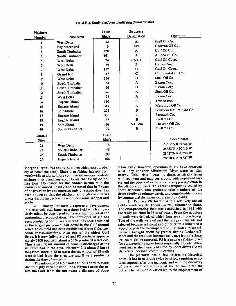
TABLE 3. Study platform identifying characteristics

Platform Lease Structure

Number Lease Area Block Designation Operator

1 West Delta 32 A Shell Oil Co.

2 Bay Marchand 3 KN Chevron Oil Co .

3 South Timbalier 128 A Gulf Oil Co .

4 South Timbalier 161 A Amoco Oil Co.

S West Delta 24 SAT-4 Gulf Oil Corp .

6 West Delta 74 F Exxon Corp .

7 West Delta 117 C Gulf Oil Corp .

8 Grand Isle 47 C Continental Oil Co.

9 West Delta 134 D Shell Oil Co.

10 South Timbalier 54 A Exxon Corp .

11 South Timbalier 66 D Exxon Corp .

12 South Timbalier 26 A Shell Oil Co.

13 West Delta 73 A Exxon Corp .

14 Eugene Island 196 C Texaco Inc .

15 Eugene Island 349 A Marathon Oil Co .

16 Ship Shoal 225 B Southern Natural Gas Co .

17 Eugene Island 330 C Pennzoil Co .

18 Eugene Island 158 B Shell Oil Co .

19 Ship Shoal 108 SAT-94 Chevron Oil Co .

20 South Timbalier 72 B Shell Oil Co.

Control Lease

Sites Block Coordinates

21 West Delta 18 29012'N x 89044'W

22 South Timbalier 46 28°53'N X 90° 16'W

23 South Timbalier 199 28°2~~N X 900 38'W

24 Eugene Island 164 28°50'N x 91 °27'W

Morgan City in 1974 and is the storm which most proba-bly affected the area) . Since then fishing has not been worthwhile at all ; no more commercial snapper boats or shrimpers visit and any sport boats that tie up do not stay long . No reason for this sudden decline with the storm is advanced . It may also be noted that in 7 years of observation by one operator only one scuba diver has been known to visit the platform although commercial divers during inspection have noticed some snapper and jewfish .

2 . Primary Platform 2 represents development in a relatively old, large, nearshore field which subjec-tively might be considered to have a high potential for contaminant accumulation . The developer of P2 has been producing for 30 years in what has been described as the largest piercement salt dome in the Gulf around which an oil field has been established (Gene Cole, per-sonal communication) . Also one of the oldest Gulf fields, it is now fully matured and P2 produces approxi-mately 5500 bpd with about a 55% produced water cut . Thus a significant amount of brine is discharged at the structure and in the area . Platform 2 is about 5 km (3 mi.) from shore in 12-m water depth . A total of 18 wells were drilled from the structure and 8 were producing during the time of sampling .

The influence of freshwater at P2 is hard to assess due to highly variable conditions . Bayou Lafourche en-ters the Gulf from the northwest a distance of about

8 km away; however, operators of P2 have observed what they consider Mississippi River water at sites nearby . This "river" water is characteristically laden with sediment and may correspond with nepheloid lay-ers and the observed occurrence of oxygen depletion in the offshore bottoms . This area is frequently visited by sport fishermen who probably take members of the drum family as primary catch, and considerable success by commercial shrimpers occurs in the vicinity .

3 . Primary Platform 3 is in a relatively old oil field considering the 42-km (26 mi .) distance to shore . The dual-producing field was established in 1968 with the study platform in 35 m of water . From the structure 11 wells were drilled, of which four are still producing . Two of the wells were oil and the rest gas . This site was selected because sediment and other criteria indicated it would be possible to compare it to Platform 1 to see dif-ferences brought about by greater depths farther off-shore and the resultant lessened influence from freshwa-ter . As might be expected, P3 is a primary fishing place for commercial snapper boats (especially Florida fisher-men) and is also heavily utilized by sport divers (Eamil Bankester, personal communication) .

The platform has a few interesting historical notes . It has been struck twice by ships, requiring struc-tural support after one incident, and with the discovery of current-induced scouring at the bottom after the other . The latter observation led to the emplacement of

27

a rock pad around the bottom of the structure . At least one sport diver has died at P3 due to a heart attack, and one other has had a severe spear injury ; both required aid from platform personnel . This is an example of the previously mentioned dependence of divers on plat-forms .

According to Bankester (personal communica-tion) this relatively offshore platform is visited by sur-face river runoff during the late winter and early spring for a period of maybe 3 months . The rest of the year the water is oceanic . An interesting point noticed by opera-tors in the field is that this area is more affected by near-shore waters than Platform 7 which is much nearer to the mouth of Southwest Pass . Bankester feels that this effect comes from a northerly direction and corresponds with current patterns which suggest more oceanic waters entering the study area to the east, holding river-in-fluenced waters closer to shore in a westward and then southward flow over the broad western expanse of the study area .

4 . Primary Platform 4 was selected by the BLM to be representative of a heavily-developed gas field sim-ilar in bottom type to P1 and P3 so that any differences effected by a gas field might be found . During the initial phases of this study it was found that workover activ-ities were to be going on at the site selected for P4 and a change was made to a nearby structure, which was used in this study . After initiation of sampling, it was found that the study platform was not primarily a gas pro-ducer though about 40-thousand cubic feet (Mcf) was discharged daily in an underwater flare . (It should be noted that underwater "flares" are actually underwater vents with no associated burning of gas .) At the struc-ture nine wells were drilled of which nearly all were oil producers and only one was still producing at the time of the study (Bill Baker, personal communication) . Platform 4 is 53 km (33 mi.) from shore in approxi-mately 46 m of water and exhibits many of the water characteristics expected in the "bluewater." Fishing is "spectacular" according to operators with much visita-tion by commercial snapper boats . It is noted that one such vessel tied up at P4 during diving operations by the study team and fished with good success .

S . Secondary Platforms 5 thru 8 were desig-nated as study sites because of their popularity as sport fishery targets . All are relatively close to the Delta area and therefore readily accessible to small boats from Grand Isle. The substrate is similar and there is a signifi-cant influence from the Mississippi River ; therefore differences between them are likely to be the results of different water depths and distance from shore .

Secondary Platform 5 (SS) is only slightly over 6 km (4 mi.) from shore in about 9 m of water . It is a sa-tellite structure, with only one well, to a very large com-plex with the highest number of nearby emergent struc-tures of any platform studied in this research . The wells in the field are largely dual producers and have been on stream about 10 years . This area was selected because it is extensively fished for nearshore species, including shrimp, trout, and drums and is near extensive oyster beds . Both charter boats and sportsmen use the struc-tures to tie up and it was noted during this study that during a period of heavy runoff numerous shrimpboats were dragging between the structures and the nearby shore ; there was also one menhaden vessel . It was the

most productive platform in biomass from trawls dur-ing Cruise II .

6 . Secondary Platform 6 is located 42 km (26 mi.) from the west delta shore in 52-m depths and was characterized during selection procedures as providing deeper water demersal species such as snapper and grouper . S6 is apparently significantly influenced by river outflow (Richard Hickman, personal communica-tion) although the extent of this cannot be estimated be-cause the line of confluence between oceanic and near-shore waters fluctuates greatly in the near area . It is noted that during the visit of this research team no red snapper were taken from this structure and the operator does not recall significant snapper fishing though an-gling for king mackerel is quite good . Though the signif-icance is unknown, at the time of sampling a large steam crane was at work removing bottom equipment adjacent to P6 . The fish fauna around the platform was "99%" blue runner (Caranx crysos) and was atypical of plat-forms visited .

7. Secondary Platform 7 was selected as a pro-ducer of both coastal and oceanic species . It is 56 km (35 mi.) from shore in 65-m depths and is located in both an oil-and gas-producing field . This relatively small field in deeper waters has been subjectively judged to hold little potential for significant contaminant accumulation, based on currents, sediment type, area production and river influence . According to Bankester (personal com-munication) it does receive surface freshwaters during the spring for a period of about 2 months .

When sampled in September, 1978 this platform showed several characteristics worthy of note . Both trawled and observed platform-associated organisms showed a high diversity, including both Caribbean and Northern Gulf faunas . The ship's Captain caught a grouper of approximately 25 kg and one spiny lobster was taken by the divers . Water appearance was quite clear and "oceanic."

8 . Secondary Platform 8 is 27 km (17 mi .) from shore in 27 m of water and was selected because of its supposed use as a fishing location for snapper and grouper . According to Alex Bisso (personal commu-nication) the structures in the area are extensively fished by commercial snapper boats, and operator personnel at platforms with living quarters take enough pompano to have a sideline business during the late fall months . These fish, taken during off hours, are shipped to shore by a commercial fisherman and end up in the restaurant trade with a value to the fisherman of nearly $2.00 per pound . This field is a dual producer and significant un-derwater flaring of gas is done according to operating needs .

This was the first platform visited after passage of Tropical Storm Debra, and two apparent results of the storm are noted . On 30 August 1978 a large gas leak was observed near Grand Isle 48-D platform, about 2 km from S8 . Trawls at S8 uniquely showed the effects of the storm . Many dead organisms such as clams were caught, but many healthy shrimp and croaker were also taken indicating recent immigration after bottom waters had mixed and reoxygenated .

9 . Secondary Platform 9 is located very near to the seaward extension of exploration in the West Delta Block in 85 m of water and about 64 km (40 mi.) off-shore . As such it is situated in a location which would indicate a minimal influence from any water except the

28

Caribbean water from the South . In addition, the field is relatively small and only seven wells have been drilled from S9, five of which were dry. Therefore, it may rep-resent the "cleanest" environment of any platform studied ; however, when visited in September 1978 dril-ling was going on and a typical mud plume was ob-served .

This platform was expected to produce deeper water demersal fish species ; however, considerable an-gling produced gray triggerfish, croaker and spotted sea trout . It is not known whether diving could have pro-duced snapper or not since this was the only platform not dived . A large hammerhead shark and muddy sur-face water conditions made diving imprudent .

10 . Secondary Platforms 10 and 11 were included in those examined during the OEI research . They are about 20 and 21 km (12 and 13 mi.) from shore, respec-tively, in about 20-m depth . Selection for the present study allows comparison of findings with respect to the differences in analytical techniques used in the two pro-grams and any differences brought about by time . Both platforms have been known to exhibit the oxygen deple-tion in bottom layers mentioned previously . They are within about 2.5 km of each other and should represent identical physical environments ; therefore, any differ-ences attributable only to platform operation should be evident . According to J . D . Murray (personal commu-nication) the one significant difference is that S10 has living quarters .

11 . Secondary Platforms 12 and 13 were selected because they were near sites of catastrophic oil spills in the past . S12 is near the site of a 1971 blowout, fire and spill of 53,000 barrels of crude oil which occurred about 600 m WSW. S13 is near the site of the 1967 spill of 160,000 barrels of crude from a pipeline break to the NW of the platform . If these large amounts of short-term contamination affect the environment some years later differently than long-term chronic pollution, this should be detectable . Both platforms are popular as rec-reational fishing spots . S12 is 11 km (7 mi.) from shore in 17 m of water and S13 is about 41 km (25 mi.) off-shore in 51 m of water .

When sampled in September 1978, S13 showed the following notable characteristics : (i) three sport fishing boats visited while on station, more than at any other, (2) divers agreed that the structure subjectively appeared to be extensively dived and (3) a large flare 600 m SW (Richard Hickman, personal communication) was burning .

12 . Secondary Platform 14 is in a large gas field and was established in 1973 . It was selected specifically to examine any effects from drilling muds in the clayey silt deposit expected to be found at the site . Twelve wells were drilled from the platform . S14 is 68 km (42 mi.) from shore located in 29 m of water . It is not expected that S14 is normally heavily fished or used for diving due to its relatively isolated location .

13 . Secondary Platform 15 is 115 km (73 mi.) offshore in about 98 m of water, the deepest platform studied in this program . It was selected to be representa-tive of recent development of a major gas field and 21 wells have been drilled at the structure . S15 is near the edge of the continental shelf and close to the limits of present production . Considering the known current pat-terns and low likelihood of terrigenous influences it is

reasonable that this platform is potentially one of the least polluted . At the time of the sampling at 515, a major platform fire had occurred and large amounts of barge and boat equipment were at the scene .

14 . Secondary Platform 16 was selected to be a counterpart to Platform 3 because of sediment type and was expected to show diminution of terrigenous effects due to the greater distance to the Mississippi River . It is located 97 km (60 mi.) from shore at a depth of 45 m . This platform is in a heavily-developed gas field and is itself a triple producer of gas, condensate, and oil . Ap-proximately 2500 bpd of oil and 300 bpd of condensate are produced and there is no underwater flaring of gas (John Simpson, personal communication) . On 4 Sep-tember 1978, S16 was observed to have an apparent leak of lighter fraction, liquid hydrocarbons which intermit-tently surfaced downcurrent approximately 10 m from the platform . The approximately 0.5 m2 sheen formed largely dissipated within the length of the research vessel as it traveled downcurrent . Several hundred meters to the west of the platform (1/2 mi . according to the Chief Scientist's Log) a large gas leak erupted at the surface . Simpson (personal communication) confirms this to be a pipeline leak in a known pipeline in the area, perhaps caused by Tropical Storm Debra which had just tra-versed the area .

S16 is reported (John Simpson, personal commu-nication) to be extensively used by sport divers and pro-duces sizeable red snapper catches for the operator per-sonnel during off hours . These fish are sold directly to two well-known restaurants in South Louisiana . Both commercial and sport fisherman also tie up here .

IS . Secondary Platform 17 is located in the larg-est deepwater oil field in the Gulf of Mexico and was se-lected in order to examine effects accrued due to that size and in the very fine, silty clay sediments . S17 is about 120 km (75 mi .) from shore in 75 m of water . It is similar in many respects to S15 and should contrast with it since differences in size and product should show up in any effects . It was expected that due to the distance from shore, fish populations at these platforms would have experienced little exploitation except from opera-tor personnel . Mr . J . M . Kates (personal communica-tion) indicates that at this deepwater platform, as well as others like it, fishing for the popular bottom species such as red snapper is not as successful as closer inshore in depths of 45 to 50 m and that bottom fish hooked are usually lost to barracuda or other predators before they can be landed . Apparently the lack of success of such fishing precludes the profitable off-hours angling re-ported at other locations . Kates reports that angling for such highly-sought sport species as cobia and king mackerel is rewarding at this platform . An interesting observation reported by commercial divers doing an-nual inspection of the structure is the long-term resi-dence of a very large grouper identifiable by a chain and shackle apparently permanently imbedded in its mouth and dangling from the jaw .

16 . Secondary Platform 18 is approximately 52 km (32 mi.) from the nearest shoreline in one of the larger nearshore oil fields in the western half of the study area . It was expected to show the effects of mod-erate pollution influences on a clayey silt sediment type . The number of wells drilled was 13 . The water depth is about 25 m, and water type was expected to be offshore with considerable influence from river inflows from the

29

East . Burgbacher (personal communication) indicates that this location has produced from 12 to 15,000 bpd of formation water which, even with the relatively good treatment at the platform, will amount to a relatively large oil discharge .

17 . Secondary Platform 19 was a special selection made to examine effects of oil production on a very sandy bottom . Moved in the initial stages of the pro-gram, the site visited is located on Ship Shoal in 6-m depths approximately 27 km (17 mi.) from shore . When S19 was visited 24 August 1978, drilling activities were going on, waves were running approximately 2 m and the water was very turbid . A unique feature of this plat-form is that the whole of S19 is built on submerged bar-ges which were used for storage of oil in the early years of production . With storage of several thousand barrels of oil by displacement of water in the barges and ship-ment every 2 to 3 days, the potential for oil contami-nation of the site appears high . In addition, when the present pipeline to shore was installed, "a whole pile of zinc" was installed . Therefore, the potential for metals contamination could be increased . Also, produced water was being released at a rate of about 9000 bpd (Bill Hanson, personal communication) . This combina-tion of high production and operational characteristics indicates S 19 as a potentially heavily-contaminated site .

18 . Secondary Platform 20 was selected for com-parison with S19 but is in a gas field . It is 15 km (9 mi.) from shore and is in about 18 m of water .

19 . Control Station 21 is adjacent to P1 and is in-termediate in location and at the same approximate depth as P2 and S5 .

20 . Control Station 22 is intermediate in location and at the same approximate depth as P2 and S8, 10, 11 and 12 .

21 . Control Station 23 is intermediate in location and at the same approximate depth as P3, P4, and S16 .

22 . Control Station 24 is intermediate in loca- tion, and at the same approximate depth as S 14, 16, 18, 19 and 20 .

D . Problems in Study Site Selection After the initiation of the program a number of un-

anticipated problems appeared with respect to site selec-tion and collection schemes for sampling locations . These problems are introduced below in order to give perspective when encountered again during review of in-dividual research efforts or synthesis of results .

1. Control Site Selection The four Control Sites selected for this program

were designated in lease blocks which had never had any exploratory drilling or development and thus were as far removed from development activities as possible, though close enough to exhibit the same sediment types, water depths, terrigenous influences and fauna as the associated study platforms . When plotted on maps of the Louisiana OCS the controls selected appear to be as good as available with respect to the platforms . How-ever, one must traverse the Louisiana OCS in a boat to get a real perspective on the amount of regional devel-opment and the difficulty in actually establishing "con-trols" which approximate study locations yet avoid con-tamination from waters passing through . In actuality it is almost impossible to lose sight of platforms on the

Louisiana OCS when at sea in good weather . The result of this concentration of production facilities shows up readily in results of this study in that "controls" are ac-tually indicative of the overall chronic contamination of the region . As such they offer a means by which individ-ual platforms can be judged for high levels of pollution ; however, none can be considered as pristine examples of undeveloped OCS .

2. Oxygen Depletion and Resultant Dead Bottoms The phenomenon of reduced dissolved oxygen

near bottom over a significant portion of the study area has been mentioned previously . This oxygen depletion is known to occur in the area on a yearly basis during spring and summer ; however, the extent of the occur-rence was apparently never documented to cover such a broad area as was found in the present study nor do as much harm to bottom populations . The occurrence caused a significant reduction in the catch of target or-ganisms at all stations where the low D .O . appeared to have exerted an influence . Figure 7, previously dis-cussed, shows those stations which showed the phenom-enon during late August and early September 1978, ei-ther through low-oxygen measurements, dead orga-nisms in trawls or absence of organisms, and a rotten egg smell to the trawl after being on bottom .

Because of the dead bottoms it was impossible to take the necessary specimens at a number of stations during the first two cruises and the catch at Controls 21 and 22 were especially impacted . Through substitutions of nontarget organisms some data were obtained, but it was not possible to obtain, within the scope of the pro-ject, the numbers needed for interstation correlations and comparisons of specific organisms and intrastation parameters .

3. Drilling and Workover Operations One of the basic tenets used in formulating the

present study was the avoidance of actual drilling opera-tions . Therefore, when these were known to occur they introduced problems . In the initial phases of the study, Platforms 3 and 4 were both identified as being candi-dates for such operations during the time of the pro-gram and changes were effected to designate new struc-tures in the same areas . During the course of the study several platforms visited either had drilling going on or were quite near to other structures with such operations . These were noted and have been considered during the Data Synthesis phase of this program .

4 . Underwater Obstructions and Satellite Platforms A significant aspect of offshore petroleum oper-

ations not readily evident to the uninitiated is the amount of underwater structures associated with gath-ering and shipment of petroleum products . Any one platform may be surrounded by a maze of pipelines, electrical cables and satellite wells which interfere with bottom currents, benthic organism migrations, and sampling of the bottom during a program such as this . Figure 13 is an example of a Primary Platform visited, showing sampling stations and underwater obstruc-tions . As can be seen, sampling stations were established in order to avoid interference with pipelines . It is obvious from examination of such a figure that use of recovered data to plot decreasing influence of a

30

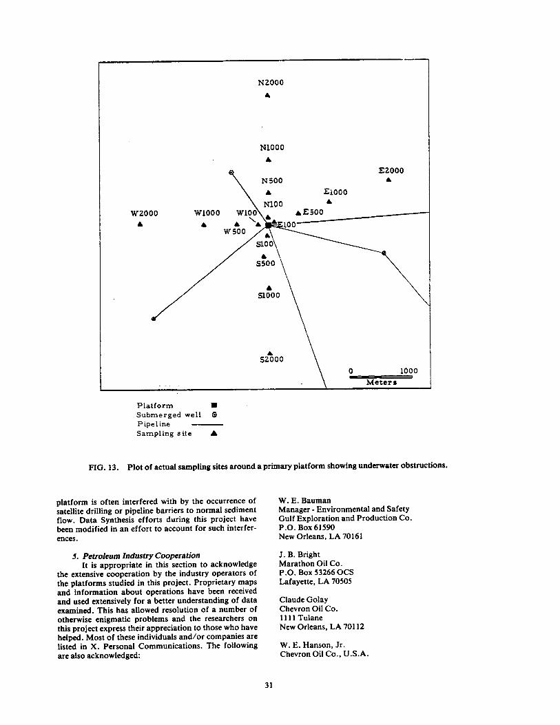
N2000

N1000

E2000 N500

E1000

N100 4V2000 W1000 W100 A AE500

100 wsoo sio\

S500\ \

siooo

s2ooo o iooo

Meters

Platform 1 Submerged well 0 Pipeline Sampling site

FIG. 13 . Plot of actual sampling sites around a primary platform showing underwater obstructions.

platform is often interfered with by the occurrence of W. E. Bauman satellite drilling or pipeline barriers to normal sediment Manager - Environmental and Safety flow . Data Synthesis efforts during this project have Gulf Exploration and Production Co . been modified in an effort to account for such interfer- P .O . Box 61590 ences . New Orleans, LA 70161

S. Petroleum Industry Cooperation It is appropriate in this section to acknowledge

the extensive cooperation by the industry operators of the platforms studied in this project . Proprietary maps and information about operations have been received and used extensively for a better understanding of data examined . This has allowed resolution of a number of otherwise enigmatic problems and the researchers on this project express their appreciation to those who have helped . Most of these individuals and/or companies are listed in X. Personal Communications . The following are also acknowledged :

J . B . Bright Marathon Oil Co . . P.O . Box 53266 OCS Lafayette, LA 70505

Claude Golay Chevron Oil Co . 1111 Tulane New Orleans, LA 70112

W. E. Hanson, Jr . Chevron Oil Co., U.S.A .

31

P.O . Box 51743 Lafayette, LA 70505

J . P . Jones Division Manager - Lafourche Division Chevron U.S.A . Inc. P.O . Box 6056 New Orleans, LA 70174

R. H . Kerr Manager of Operations Southern Natural Gas Company P.O . Box 1513 - Richmond Tower Bldg . Houston, TX 77001

L . L . Keyes Advisor - Environmental Affairs Gulf Oil Exploration and Production Co. P.O . Box 61590 New Orleans, LA 70161

Neville J. Ory Sr . Civil Engineer, Offshore Division

Texaco, Inc . P.O . Box 60252 New Orleans, LA 70160

John A. Queen Director - Environmental Affairs Continental ~M'Company 5 Greenway Plaza East P.O . Box 2197 Houston, TX 77001

F . E . Syfan Production Coordination Superintendent Amoco Production Company 1340 Poydras St . P .O . Box 50879 New Orleans, LA 70150

C. Rupert Turner Division Manager Shell Oil Company One Shell Square P.O . Box 60124 New Orleans, LA 70160

32

VI . SCOPE OF WORK

A. Field Sampling Program

1. Sampling Cruises The design protocol for the pollutant fate and ef-

fects study called for three sampling excursions-one during each of the three ecologically distinct seasons of the northern Gulf of Mexico spring, late summer/early fall, and winter. Because of delays in contract award the first cruise was delayed ; thus the actual sampling times were May, August/September, and January . Initial plans were to conduct all sampling from one vessel dur-ing each season except for the diving effort during the Artificial Reef Studies . This effort was planned to in-volve a separate cruise because of the special needs for diving support, and since it was a one-time-only sam-pling effort, June was chosen to maximize water and weather conditions .

After the first sampling cruise it was obvious that plans to take biological samples by trawls and angling required special equipment and flexibility not possible under the proposed plan ; therefore, a special cruise was taken during August/September with a smaller scien-tific complement using a shrimpboat to take all trawls and for angling and diving at platforms to take structure associated species .

After sailing on the second cruise to take bottom samples, weather forced interruption of activities and because of continuing difficulties in navigation and po-sitioning caused by a ship's crew inexperienced with sci-entific requirements, it was decided to terminate the cruise . The remaining sampling requirements were ful-filled on a second leg on a different ship .

Because of the various times and separate legs of cruises to fulfill requirements, a nomenclatural conven-tion has been adopted in referring to the sampling trips taken for the Fate and Effects Studies . The spring cruise, May 1978, is called Cruise I in this report . Cruise II, August/September 1978, is split into three parts, A, B and C, according to the times of departure of the various vessels . Legs II-A and II-C were for the taking of hydrographic and sediment associated samples . Leg II-B was the "fishing" trip for trawling, diving and an-gling . Cruise III is the winter 1979 excursion .

The dates of the various study cruises and the vessels used for each are listed below:

Cruise I (May 20-June 2, 1978) Sea Trans-porter, Santa Barbara, California ;

Cruise II-A (August 17-28, 1978) T-Kip IV, Free-port, Texas ;

Cruise II-B (August 21-September 6, 1978) Tonys and Joe, Freeport, Texas;

Cruise II-C (September 15-25, 1978) Sea Trans-porter, Santa Barbara, California ;

Cruise III (January 4-16, 1979) Sea Transporter, Santa Barbara, California .

2. Sampling Patterns Primary Platforms 1-4 were visited in each of the

three seasons and sampled for a complete spectrum of parameters at 16 locations around the platform . These stations were located on the four axes of the compass at

distances of 100, :500, 1000 and 2000 m from the study platform in an idealized "bullseye" pattern to account for any buildup of contaminants in samples ap-proaching the platform . In actuality the underwater ob-structions caused by pipelines and satellite structures dictated that samples be taken at some deviation to the idealized grid . Figure 13, previously discussed, is the ac-tual plot of one such set of samples and and the bottom structures which dictated changes in the plan . Though actual tracks of pipelines and underwater cables is not known with certainty at most locations, maps of these conditions have been received from the operating com-panies . From these maps approximate distances from sampling locations and obstructions were determined for use in estimating potential influences from bottom perturbations . This information has been used in Data Synthesis tasks but these maps are not included in this report due to their proprietary nature .

Secondary Platforms 5 through 20 were sampled only on the North transect at 100, 500, 1000, and 2000 m according to the same protocol for avoidance of in-terfering structures . Sampling at secondaries was done on the late summer expeditions, Cruise II .

Control sampling locations were selected to ap-proximate environmental conditions found at nearby platforms yet were in lease blocks which have not expe-rienced any exploratory or development activities . Pop-ular knowledge indicated that selection of "pristine" controls in the Louisiana OCS would be impractical and these selections are a "best effort" at finding appropri-ate comparison areas for the study sites . Controls were sampled during each of the three seasons .

3. Samples Taken A complete description of the individual samples

taken in this project would require extensive space . Therefore, a Master Sampling Scheme as used on-board ship is reproduced in Table 4 . It includes all samples to be taken in each of the three collections . Parameters studied as disciplines are listed according to their segre-gation into Work Groups or subcontracts for the study : (1) Hydrography ; (2) Sediment Physical Characteriza-tion ; (3) Organic (Hydrocarbon) Chemistry of Water, Sediments and Fauna; (4) Trace Metal Chemistry of Sediments and Fauna; (5) Microbiology of Sediments ; (6) Histopathology ; (7) Benthic Faunal Populations ; and (8) Artificial Reef Studies . As is readily evident, the logistics necessary to insure taking of all required sam-ples, tagging, inventorying and transshipment to insure accurate delivery was formidable . It was accomplished by using preprinted sampling logistics logbooks and du-plicate labels to give cross checks as samples were taken, and by rigorous inventory controls as samples changed disposition during the course of study . Sample Control Inventories were 'maintained by the Data Manager in an effort to account for any sample's whereabouts at any time .

The various Parts of this report detailing find-ings by discipline ; give a comprehensive accounting of the kind and number of samples analyzed, as well as the sampling location and season . This information is also included in the data summaries in Volume I, Part 8 .

33

TABLE 4. Master sampling scheme for each Primary Platform, Secondary Platform and Control Site

SDrini ~mplini 1- 1978 IADri1~MlY1

Pu~mtlm PomaryPINfwmsSunpling Swoons

r~ " ~^"" loco mm w Imo wo noo im wo imo m ~w s,yr ... .s..ri .~

% x K r . ~ia..r r.~..

< s~ssr~ef.'q-

ArrsrrWi Frlwi.

~ uwn .~uN+V

1 hlywfMn-Irr~ 4w~Y

I ",ly~YWS-MMr'-No

SupN

" ~ ~ ~ Icti I<G

~vMVwW~1~

' f!G 1RG

' ~nM-!rte

~HSnr " i

° iHSnr "

w~uw.,w �~. xHSnr

~ MeeI~YW ww Su~NiN

uuno~ Iron p~bll:~ u~qn~TS~

eumqnlran,~r w~i~i

.,mqn

34

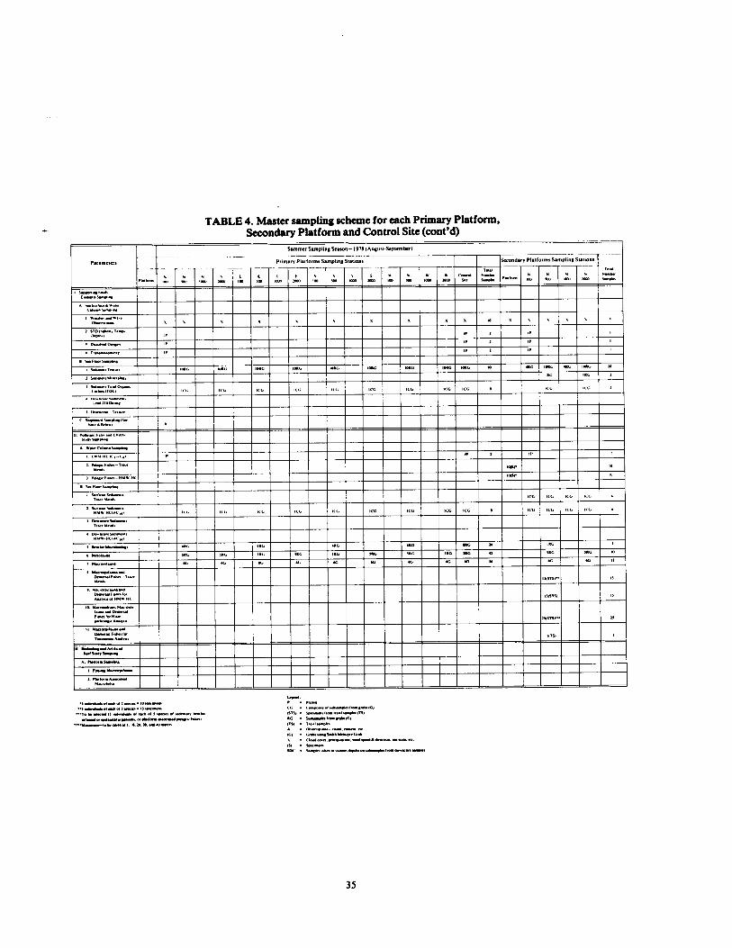
TABLE 4. Maser sampling scheme for each Primary Platform, Secondary Platform and Control Site (cont'd)

s- s.mouiss sh- 1918 (A. a.-s.ol-een =----

Pu~memrs PrimuyPluformsSampIins Station, SecondaryPlulormsSamDIing SUiions -

_ _.

ilw

..

p y~ aiN

`Sw

TaW

N~r1~ S~yl~

~a - .bo~ ~LnOw

I SYVK~~~Yf~Wr M~i~sunM~4

1~ x 1. 3 Sp7,Oq^fJ-itip

~ Ss mrS~~pY~i

i rrYYr

~-tarot

t 9lysraL~pw1]ae

"S~+T~rWY IIRi~

...vnp~

I . =-- i4iP

Mw

7 ~Ny~iw~n-NN<, ms .

ibaSSN~a

1 u rye .

YnarqqY

Is. Is. Is. I.G .1 Is .

eM-Trr If15731""

iHSrn

w~wwr+.~r." ~i w.. ..a a

..,~ .~rrM..ia

11. Wwj~Y~rulr~l ~wILWf s~pY

w. M~n~SrNy

I . faYy WeiaAlri

lib'

qrwupnlra V~a1G1

F"r1sr11f ~N~"W N M M y~ .~ M vJn~rY err " sR~e~Ir~in~IrY~1751 " ~IWoqnirYa~r+w .o~Ylar~mrNO4yrw-le~ni - LwrN~tayY~lcl

wtrWwui .to.70.10.Wauwar. ~.i,rpn

w~V+wa~"~ayraa~ia~ .svue.u . 5y�,r�

SM . yip�u~nu .vowW~wuw~retiua~aw~mir~lu

35

TABLE 4. Master sampling scheme for each Primary Platform, Secondary Platform and Control Site (cont'd)

W ieter Sampling Season-1979 (hnuur-Felruuy)

Puialetvi Primary Platforms Sarnplins Stations

rw~>. moo wo t

wm s iao

s iano ~m foo loos

ca..r fw s.nr

i . ~w .~~ .,arr ssnasna

A . s.s.n.o.~v.�. rr ~..w rM W vin

I OYn.wer

TOISYYiYi~ I qM~~I

--On- 11

v

7

t. 7~ ilm y hliy

10~G

ICG ICG

". Owes Srrw~ 1~07~Op~ly

f. Pwv~-imv~

c . a~~~...ya.

n . r.r+rr.ereiM. vrrsr.w

ww ~. iaw~rw-Hrv.wc

~ . s . rw ~�r i . vreraw~....

~ .. wo` ~. ~.rtusr.~~

oe.~a.v~,..

rr4.+.~wr .~c nc Is. In.

b

t. Ilsrw~ilxri W MrrW fYn-Trrt

~wwaNYV-NC

ia.11r~w

piMYp~Wrw

II . WnaM~rW

NYrW

11. YNSIy W Mti~ 4~IiHr~Y

A.'Yls~frjYy

L fwYy4~oapir T ~

I 1 I ~ I~

/

~I ~

,

~I

soc - s..w "w. ...w..r,~r . . .w..rer.~r....n.ri .

36

4. Sampling Gear and Use A detailed discussion of sampling for all parame-

ters is not warranted in this discussion as particular con-tamination problems or sample recovery techniques are covered in each Part of this Volume. A general narrative of the gear used and its deployment is given in order that the reader may better understand shipboard controls of sample taking and logistics.

Three primary sampling regimes were followed in procuring analytical materials: hydrocasts for water column physical description and samples, piston corers and Smith-McIntyre grabs for sediments, and "fishing" activities including trawling, angling and diving for re-covery of demersal fish and invertebrates and platform associated fauna. The first two activities were best car-ried out on one vessel while fishing required another.

a. Water Column Sampling Water column sampling and hydrography

were a minor part of the overall sampling program . It was not within the scope of the study to incorporate enough hydrography to comprehensively depict area conditions ; therefore, limited sampling was done to show gross conditions at the North 100-m (N 100) sta-tion at each platform . Hydrocasts took data at 1-m under the surface and at subsequent 10-m depths until the last bottle was within 10 m of the bottom . At each depth water samples were taken with a GO-FLOG (General Oceanics, Model 1080) water bottle for sub-sampling and shipboard analysis of salinity and dis-solved oxygen . Temperature was taken with a reversing frame thermometer (Watanabe, -2 to 35 C) and trans-missometry data was taken with a 1-m-light-path Hy-droproducts (Mode1412-0001-1) instrument .

In taking hydrocasts standard procedures were used to insure sampling at the proper depth and special pains were taken to avoid contamination . Hy-drocasts were taken with stainless steel cable which was precleaned with hexane solvent and frequently recleaned during use ; the a-frame, block and retrieval area were kept clean, and personnel were indoctrinated with the precepts of hydrocarbon and trace metal contamination avoidance . GO-FLOG samplers, from which contami-nant samples were removed, were always cocked and subsampled inside the on-deck wet lab ; therefore, the inside of the water samplers was exposed to the environ-ment only after entering the water's surface and upon being opened for draining inside the wet lab .

6. Sediment Sampling By far the most labor and time intensive of

any activities at sea on this program was the extensive sampling of the sediments for contaminating hydrocar-bons and trace metals, infaunal biological collections, and downcore sampling for contamination with age of sediments . The principal tool used in this work was the Smith-McIntyre Grab (Kahlsico Model 214WA250) from which cores and surface samples were removed as necessary for the various scientific disciplines . Each Part of this report details any appropriate subsample and its recovery from the grab . The other important tool used in sediment recovery was a 1-m piston corer (Kahlsico Model 217WA260) . A number of difficulties arose in connection with this activity and will be dis-cussed later under the section on Problems in Sampling and in the various appropriate disciplines .

Operation of the Smith-McIntyre Grab is rel-atively simple and does not require explanation . Some aspects of its use important to the success of the study are given here. When on a station at a platform, succes-sive drops of the grab were made as rapidly as practica-ble using a team approach to operation and sample re-moval . Shifts were run on a 24-hour basis to insure the best return for resources put into ship time . A two-man team armed the grab, retrieved it and did subsampling for those parameters not requiring contaminant protec-tion, such as benthic organisms and sediment grain size . If samples taken at a station required protection from airborne contaminants, the grab was retrieved and swung into position on a "porch" to the wet lab . This wet lab had a large "antechamber" which could be swung like a door into position over the grab to protect it from airborne contaminants . Once the grab was inside this antechamber, the wet lab was opened and two scien-tists inside proceeded to open the grab and remove sub-samples . The lab was an aluminum building fitted with a self-contained water sampling and grab subsampling lab . It was air conditioned and had a positive pressure air-filtration system . Sampling, labeling, inventorying and temporary storage of samples were done in the pro-tected environment of this lab or the antechamber . After subsampling, all remaining sediments were trans-ported to the fantail of the vessel for complete sieving by the benthic biology team .

As in all sampling, the grab was given special treatment to curtail contamination. Prior to going to sea, it was washed with detergent, then solvent and acid and stored clean . Stainless steel cable was used and fre-quent washings took place at sea .

Measures were also taken to audit trace metal and hydrocarbon contamination . Samples were taken of items which might have led to contamination at time of collection . These samples included scrapings of paint chips, which were analyzed for trace metals, and sam-ples of bilge water, engine lubricating oil, fuel and other lubricants for hydrocarbons fingerprinting . Through this audit of potential contaminants a file was developed for comparison should results from sample analysis in-dicate shipboard contamination . No contamination was ever encountered .

Downcore sampling for recovery of sedi-ments to be used for dating of the sediments and subse-quent contaminant analysis with age was attempted with the piston corer . Operation of the corer was according to protocol, which called for solvent-washed aluminum liners for taking of cores for hydrocarbon analysis, acid-washed LexanOO liners for cores for trace metals analysis and a third core for dating by the lead-210 method . Cores were taken to at least 50-cm depths whenever possible .

c. Epifauna and Fish Sampling Collections of organisms for contaminant

histopathological and benthic population analysis in-cluded demersal organisms and platform associated biota. These were taken in three ways ; trawling, angling and diving . Trawling was done with 9-m (30-ft.) otter trawls copied from nets used on the MAFLA program and similar to those used on the STOCS work in order to correlate catches as much as possible . Except for the following steps taken to avoid contamination, the trawl-ing program was carried out according to methods used

37

during normal shrimping operations . Trawls were con-structed of nylon and left untarred . Stainless steel bri-dles and cables and a tickler chain tied in a "Texas drop" were used . Equipment was washed and stored in clean wooden boxes during shipping and when not in use . Trawls were washed with detergent and well rinsed with seawater immediately before use and towed at depth for infrequent washings . When recovered on deck trawls were emptied into stainless steel trays which re-ceived similar washings and were frequently rinsed . Or-ganisms for trace metal determinations were handled with acid-washed rubber gloves and those for hydrocar-bon testing with stainless steel tongs . Further on-deck treatment included packaging in clean, noncontaminat-ing materials according to contract protocols, further explained in each appropriate Part of this report . The preprinted labels, inventory and accompanying logs in-sured adequate sample disposition control .

Angling was done at platforms in order to catch pelagic species which associate with structures ; red snapper and groupers were the target organisms . A number of problems arose with regard to this effort and are further described under the problems section . Spe-cial efforts were made during angling to avoid contami-nation . Stainless steel hooks were used and fish were re-moved with pliers or gloves as necessary . Immediately upon retrieval fish were placed in ice chests which were prepared for receipt of trace metals samples by being acid washed and for hydrocarbon samples by being lined with hexane-washed aluminum foil .

The diving effort recovered organisms using stainless steel equipment and organisms were treated as described above when recovered on deck .

S. Problems in Sampling

a. Positioning and Relocation of Sites In the proposed protocol to BLM, SwRI

planned to use horizontal angles, obtained with a nav-igation sextant, as the primary means of positioning . It was believed that except for the control sites (at which positioning would be by Loran A) the required posi-tional accuracy of t50 m could be obtained with a sex-tant . A costly precision electronic navigation system would not be necessary.

Following discussions with BLM, it was de-cided that Decca Hi-FixO would be utilized on the first cruise along with the sextant . A comparison between positioning with the sextant and the Hi-FixO would be made . However, due to the greater than anticipated manpower needs to operate the Smith-McIntyre Grab, the Chief Scientist and Oceanographic Technician did not have the time to devote to the sextant positioning that the situation required . At most stations, only the Hi-FixO was used .

A few trials with the sextant were made. They indicated that with experience it could be used for preci-sion positioning . Problems were encountered locating reference points on the platforms while looking through a sextant . The massive structures all looked alike in the narrow, overlapping view through a sextant and the multitude of lights on the platforms and vessels obscured the platform navigation lights . The greatest problem was in rapidly obtaining two cross angles in a short enough interval so that the drift or movement of the vessel in this interval had a negligible effect on the measured angles and resulting fix .

In addition to its expense, deficiencies in the Hi-FixO were its several breakdowns and its near nightly shutdowns due to atmospheric conditions . Both of these problems required frequent, lengthy diversions to a platform with a known position for recalibration of "lane count."

Many of the problems with navigation had less to do with the positioning system than with the nav-igating (conning) of the ship around buoys or close in around the platforms . Hi-FixO, sextant angles, pelorus angles and radar could have adequately positioned the ship . But, at those stations where it was not possible to anchor the ship, the drift between the time the navigator said we were "there" and the time the sample was actu-ally obtained could exceed 50 m. Unfortunately, there were a considerable number of stations where it was not possible to anchor . Because of the proximity of the plat-forms and the presence of obstructions, it was not possi-ble to anchor at any of the 100-m stations . Additionally, the problem there was compounded by the fact that a buoy could not be put over because it would obstruct the ship's approaches, the platform inhibited proper up-wind approaches, and the Hi-FixO was affected by the platform structure at that range . Anchoring at any sta-tion at Primary Platform 2 was prohibited .

In discussions with BLM following the first cruise, it was decided a new but potentially highly capa-ble navigation system would be used . Two Variable Range Marker units (VRM) would be installed on the ship's existing radar and the ship positioned using si-multaneous ranges off of nearby platforms . At least two platforms with known positions were within a short enough distance of all sampling sites to permit accurate range/range positioning . In most cases there were plat-forms near enough to permit using the 1/2-mile range on the radar and in all cases within the 1-1/2-mile range . The Paragon0 VRM's could be set to 10.01 nautical miles (118.4 m) for distances up to 1 .90 miles and t0.1 nautical miles (1184 m) for up to 25 miles . Using radar echoes off platforms with known positions made it un-necessary to put transmitters on the platforms or rely on distant shore stations .

In operation, the radar presentation of the target platforms, the ship's headings, and the two VRM rings, which have been pre-set to the appropriate ranges from the sampling stations to the target platforms, gives the helmsman an appreciation of position and the course to converge on the correct position .

VRM units to be attached to an existing radar are relatively inexpensive and the ship's officers can quickly learn the system . With their appreciation of their ship's handling characteristics, they can quickly get on station . Thus, appreciable economics can be real-ized . An additional, skilled navigation team with their expensive equipment is not required aboard the ship or ashore .

Figure 14 shows the geographic representa-tion of the range/range positioning mode and the radar presentation when the ship has arrived on position . The VRM rings have been set to the range R, and RZ as de-termined from the geographic presentation utilizing tri-gonometric computations . The false location can be avoided by observing the relative positions of other plat-forms or by geographic bearing from a platform utiliz-ing the ship's compass .

38

Station P2

False Lototlon R

0 P7

Geographic Representation

FIG . 14 . Geographic representation of a range/range positioning mode and radar presentation of ship on location when using variable range marker (VRM)

positioning .

The Dual VRM system was very success-fully used during Cruises II and III with no failures of the Paragon0 units or the Furuno radars to which they were connected . Positioning at all stations was accurate and rapid . The only thing the scientific staff had to do before arriving at a station was to set into the VRM's the two pre-computed ranges and then assist the helmsman in locating the proper platforms among the myriad of platforms and vessels frequently visible on the radar screen . Many times upon approaching a sta-tion the vessel could be put into position in less than a minute .

b. Downcore Sampling with the Piston Corer The "downcore" sampling effort was an at-

tempt to recover three identical cores, 50 cm in length, at each Control Site and at N 100 at each Primary Plat-form . Much difficulty was encountered in making the piston corer work properly to the SO-cm depth . Cores were taken numerous times and one corer was lost be-fore a suite of marginal cores were recovered . The real reason for difficulty in coring was never determined though a number of hypotheses include: poor fabrica-tion of the instrument which precluded smooth action of the piston ; not enough weight ; too much weight ; the taking of extremely unconsolidated sediments which went out the top of the tube; and the attempted taking of very compacted elastics which compressed rather than enter the tube . All or none of the above may be correct in the experience of the Program Manager .

In addition to the recovery of a marginal set of material, analyses were unrewarding . Lead-210 dating did not show any layering with time in any of the cores examined down to 50 cm and in fact gave evidence that sediments were particularly well mixed . (This is consistent with what the research team has learned in retrospect.) Hydrocarbon analysis was curtailed to a minimal effort due to the irregularity of sedimentation ; however, the analyses indicated, if anything, enrich-ment with depth . This is more fully discussed in Part 3 . Trace metals analysis also showed complete mixing and is discussed in Part 4 .

c . Trawling The primary lesson learned during Cruise I

with regard to trawling was that it is best done from a boat designed for that purpose . Trawling from the shrimpboat was no problem and samples were recovered with reasonable ease where enough of the target orga-nisms were available . Low dissolved oxygen concentra-tions, resulting in "dead bottom" conditions, precluded success at a number of locations . One note for future reference is that nets left untarred or not coated with plastic come untied easily . Therefore, all knots should be double tied in the webbing . Several trawls were lost to bottom snags during this program, and on the sum-mer cruise emphasizing biological sampling all four trawls designated for the program plus the ship's trynet were either lost or badly damaged . On one occasion, as shown by fathometer tracings and condition of the re-covered parts, a trawl was torn on a clay bank . On an-other occasion fathometer tracings and catch indicated that we were following a pipeline when the trawl became hung and was torn . Most problems with hangs and trawl damage occurred in deeper water and by the end of sam-pling on Cruise Il :-B at the far offshore stations we had effectively destroyed the nets . Our brief experience indi-cated that both natural and manmade obstructions may cause loss of fishing gear around platforms .

d. Angling at Platforms As has been previously mentioned, angling at

platforms was initially intended to be done from the sin-gle vessel used in .all Fate and Effects sampling . A small boat was launched from the main vessel and fishing was done at the platform from it . The logistics in launching and recovery and the time spent in unproductive fishing efforts proved during the first cruise that another ap-proach would have to be tried . The "fishing" trip de-scribed previously as Cruise II-B had as a primary pur-pose angling at platforms to catch all possible of the tar-get or secondary species, snappers and grouper, then spadefish and sheepshead or others, respectively, then to take whatever species were available during diving to round out contract requirements for numbers of orga-nisms . This special cruise was costly but was reasonably successful in taking organisms where any existed .

e. Low Dissolved Oxygen Levels With regard to sampling activities, the low

dissolved oxygen and dead bottom conditions encoun-tered in Cruise I and Cruise II caused particular prob-lems in shipboard decision making . Resources were ex-pended at high rates while continued efforts at trawling or angling for target species were fruitless . Decisions had to be made as to when to stop trying for designated organisms and start substituting others, then decisions had to be made when continued trials produced

39

Radar Presentation

nothing. It was largely because of the low dissolved oxy-gen that Cruise II-B was designed in order to minimize resource expenditure by using a smaller vessel and a considerably reduced crew .

Other problems and unexpected conditions caused considerable adaptation of proposed techniques during actual operations and are discussed where appro-priate . In general, they caused little interference with ul-timate sample delivery however large they were consid-ered at the time of encounter .

B. Analytical Program

1. Shipboard Analyses Because of the multiplicity of sampling and the

elaborate analytical schemes necessary to complete ex-amination of most samples taken, little analysis was planned or completed onboard ship . Instead, most sam-ples were fixed, frozen or otherwise preserved for trans-port to the proper lab . Some onboard analyses of hy-drographic parameters were done . These included the hydrocast measurements and analyses of GO-FLOG samples for salinity (Plessey Model RSS-3 Laboratory Salinometer), temperature (reversing frame Watanabe -2 to 35 C thermometers), dissolved oxygen (Winkler method) and transmissometry (Hydroproducts, Model 412-0001-1 transmissometer with 1-m light path) . Stan-dard observations of wind and weather were recorded in the Chief Scientist's Log.

2. Laboratory Analyses Each Part of this report details the pertinent as-

pects of laboratory analyses of samples . These descrip-tions validate the underlying principal of using the most current techniques in the study . As important circum-stances of analyses such as incompleteness or error in re-quired technique were identified, they were noted for use in comparison with depth of findings, comparison with other parameters, implications for future research and validity with respect to study goals .

3. The Problem of Contamination This study embarked on cruises in relatively

clean waters and bottoms in an effort to pinpoint ex-tremely low levels of pollutant contamination . In order to do this, extreme measures were taken to prevent sam-ple contamination from sampling gear, sample con-tainer preparation, on-deck handling procedures, logis-tics and shipping, and laboratory processing .

Steps taken to prevent contamination were bro-ken down into two categories : prevention of hydrocar-bon contamination and prevention of trace metals con-tamination . Within each area of contamination preven-tion, efforts were directed toward two types of collections : physical and biological . In general, cleanli-ness was the overall key to prevention of contamination, with all equipment and containers rinsed with an

organic solvent (hexane) to limit hydrocarbon contami-nation and with acid (sulfuric) in the case of trace met-als .

For sampling of the water column all-plastic GO-FLOO samplers were chosen since they could be low-ered from the surface in a closed mode, then opened at depth . Frequent hexane rinses assured clean samples . Sediment samples were taken in two ways, the Smith-McIntyre grab (Kahlsico No . 214WA250) and the piston corer (Kahlsico No. 217WA260) . From each grab, sub-samples were taken for a number of parameters includ-ing hydrocarbons and trace metals using stainless steel and polyacrylic corers, respectively . Sediments at each Primary Platform were sampled with the piston corer using both stainless steel and plastic liners, for the same parameters but at deeper depths .

Biological samples were taken in a variety of ways depending upon the organisms' habitat : with grabs, trawls, angling and by spear . In general, any metal gear used was stainless steel when possible, e.g ., the Smith-McIntyre grab, hooks, spear points, etc . Trawls were of uncoated nylon as was the bag used to sack speared fish underwater . When biological samples arrived on deck, they were either sorted in a washed, rinsed, stainless steel trawl tray or went directly into alu-minum foil lined or washed plastic ice chests prior to la-beling and storage .

This writer perceives that, in the time that sam-ples are on deck prior to storage, the greatest threat to contamination is from diesel exhaust . In this program, emphasis was given to covering samples and processing them rapidly . The major covering for physical samples was the on-deck laboratory whereas biological samples were generally kept in ice chests .

Storage containers followed the basic format of plastic for metals collections and aluminum-lined for hydrocarbons . Because internal tissues were so often the material used in analyses, these measures, along with the natural protection of the organisms' covering, pre-vented any contamination in samples analyzed .

In the laboratory the same theme of general cleanliness allowed control of contamination . Desig-nated areas were set aside for sample preparation according to the type of analysis ; clean benches with hoods and glassware and tools dedicated to that phase of the project were used . Designated individuals per-formed the same tasks in a series of analyses and logs were kept to document standard operating procedures from step to step .

To check for possible contamination of samples, checks in the form of blind quality control samples of duplicates and "doped" containers were set up and samples of potentially polluting ship's bilge, engine oil and paint chips were taken for cross reference . As a re-sult of these intricate controls and elaborate quality checks, no contamination from sampling activities has been identified .

40

VII. DATA MANAGEMENT

Data Management was responsible for the coordina-tion, systematization, and centralization of activities with respect to data recording, summarization, utiliza-tion, and reporting of final data to BLM and National Oceanic and Atmospheric Administration-Environmen-tal Data and Information Service-National Oceano-graphic Data Center (NOAH-EDIS-NODC) .

Some of the more important tasks to be discussed below are:

" Standardization of data reporting procedures " Development of a sample coding system " Sample and data inventory control " Data base design and management " Validation, reduction, and summarization of sci-

entific data " Distribution of data to data synthesis groups " Submission of data on magnetic tape to NOAA-

EDIS-NODC

A. Sample/Data Inventory and Control A sample/data inventory control system was devel-

oped to monitor progress, to identify any missing sam-ples or data, and to signal any further sampling or data processing requirements . These control procedures were then used to document the status of data availability, data processing, and data analysis at each reporting pe-riod . Sample inventory control and data inventory con-trol were similar-the sample inventory control was fo-cused upon the sample collection and the data inventory control was an extension of the same system tracking the sample and data through the remainder of the ana-lytical and data handling stages .

TABLE S . Sa

Both the sample inventory control and the data in-ventory control procedures depended upon a unique sample identification system . The coding system devel-oped is shown in Table 5 . This 20-character sample code is used to uniquely identify each sample and subsample collected and analyzed during the project . Not only does the coding provide for sample labeling, but it also re-mains with any and all data that derive from that sample or subsample .

The coding system is heirarchical in content supply-ing the when, where, what, which, how, and who infor-mation necessary for proper sample and data handling . The year and month of sampling is given in the first four characters . The next eight characters explicitly designate the sampling station . The next three characters (13 to 15) indicate the particular sampling element or study-see Table 6 for code definitions . The next two characters (16-17) serve to identify the sample and subsample if any . The final three characters (18-20) indicate the dis-position of the sample in terms of the type of analysis to be performed and what laboratory is to perform the analysis .

A system for labeling samples at the time they were gathered was developed . This labeling system was the basis for the proper collection, subdivision, processing, and laboratory distribution of the samples, and for the proper identification of the laboratory data . A distinc-tion should be made between the sample identification code and the sample label . The sample identification code is designed to carry complete information about the sample, its type, its origin, and its disposition . So defined, it is intended to be readily decoded but not nec-essarily easily read . The sample label, on the other hand, is designed so that pertinent information for

mple coding system

Code Possible 'olumn Information Codes 1-4 Sampling season S-6 Platform/Site number 7 Platform/Site type C

P S

8 Transect N E S W

9-12 Distance noon 13 Sampling study 1

2 3

14 Parameter group A-C 15 Parameter subgroup 1-9,A-B tb Sample/grab number 1-9,X 17 Subsample identification A-E IS Analysis classification A

C P T M H

19 20

Unused Analysis laboratory G

J T H M B S L

41

Year and month in form yymm 01 to 24 Control site Primary site Secondary site North East South West 0100, 0500, 1000, or 2000 Supportive Pollutant fate and effects Biofouling See Table V-2 See Table V-2 (varies with usage) (varies with usage) Biological Chemical Physical Taxonomic Trace Metals Hydrocarbons

Geochem Sw R l -Hydrocarbons SwR1 Trace metals TAMqJ-Sediments MSU-Microbiology SwRI-Benthic TAM U-Histopathology LGL

TABLE 6. Study element codes by work group

Code Parameter group WORK GROUP 4 .COOPER

IAI Weather and Wave IA2 STD IA3 Dissolved Oxygen IA4 Transmissometry ICI Shipboard Sampling

WORK GROUP 5 -GEOCHEM 183 Sediment TOC 2AI LMW-HCinWater 2132 Surficial Sed . -HM W-HC 2114 Downcore Sed. -HMW-HC

WORK GROUP 6-NULTON 2A3 Pelagic Fishes -HMW-HC

WORK GROUP 7 -TILLERY 1114 DowncoreSed.Pb210 2A2 Pelagic Fishes - TM 281 Surficial Sed . TM 2113 Downcore Sed. - TM 288 Mac. & Dem. Fish TM

WORK GROUP 8 -HUANG 1B1 Sediment Texture IB2 Sediment Mineralogy

WORK GROUP 9-BROWN 2135 Benthic Microbiology

WORK GROUP 10 -BAKER 2116 Meiofauna 2117 Macroinfauna 2138 Mac . & Dem . Fish -Tax . .

WORK GROUP 11 -SIS & ARMSTRONG 2BA Histopathology

WORK GROUP 12-LGL 3A1 Fouling Macroepifauna 3A2 Platform Macrobiota

sample collection, handling, distribution, and analysis is instantly recognizable . It is obvious that all information in the code is not necessary to sample handling, but the entire contents are pertinent and necessary to data hand-ling . The labels were printed in the sequence that best facilitated their attachment to the sample containers . The set of labels for each sampling cruise was provided to the field crew 1 week prior to each cruise .

The computer programs which generated the sample labels printed, in addition to the labels, several sets of sample inventory check lists of the proper sample codes based upon the predetermined distribution of the sam-ples . Copies of the appropriate check lists were provided to the field crew who first used them to insure that all labels and sample containers were available . While on-board, the check lists were used to organize sampling . As each sample was collected, it was so noted on the check list . At the conclusion of the cruise, the check lists were used to inventory the collected samples and also to indicate the disposition or distribution of each sample . The check lists were then forwarded to the Data Man-ager .

Using these check lists Data Management then up-dated a master sample/data inventory data base to re-flect the actual sample inventory for the respective cruise . From this data base the sample inventory report was prepared .

Appropriate sample receipt forms were sent to the recipients of the samples at least 1 week prior to the ex-pected sample receipt . The completed forms were re-turned to the Data Manager and were used to update the master sample/data inventory file . Using this data base and its associated programs, a quarterly data inventory

report was prepared for attachment to the Quarterly Summary Report . This report detailed the status of sample processing, distribution, analysis, data entry, and data base storage.

B. Data Entry System All data entry was done using a key-to-disk data

entry system which SwRI has assembled and developed over the last 5 years . The advantages of a minicom-puter-based, cardless, and interactive data entry system with dynamic data editing and manipulation at key-in time are obvious . Table lookup permitted easy vali-dation of station identifiers, dates, or destination codes for example. The National Oceanographic Data Center (NODC) Taxonomic Code was obtained on magnetic tape, and was installed on the minicomputer system . Over 26,000 taxa are included in the current version . This system provides the degree of standardization of taxonomy required by the contract .

The NODC code provides for six levels of classifica-tion with a two-digit numeric code for each level. A thir-teenth character is also utilized by NODC to indicate synonyms or alternate names. Thus, an organism can be uniquely identified by a 13-digit number.

A subset of this taxonomic catalog was developed and maintained for use in this project . Dr. Baker of the benthic biology work group assisted in the construction and maintenance of this catalog . When taxa were en-countered for which there was no NODC code, a tempo-rary code was assigned with the thirteenth character containing an asterisk to label it a temporary code . Taxa with temporary codes were then submitted to Dr . Elaine Collins of NODC for assignment of permanent codes .

C. Data Base Management Systems A combination of in-house and external hardware

and software was utilized for efficient and economical data processing and data base management . All data ed-iting and file management was accomplished on the in-house minicomputer system . In this manner, clean and properly formatted data sets were then transmitted via remote batch to a large computer data base manage-ment system (DBMS) . The two systems were comple-mentary and provided the overall cost efficiency and se-curity redundancy required . The approach was oriented toward increased computer utilization and reduced manpower requirements .

During the project there was a shift towards less use of external systems and increased utilization of the in-house systems . The primary reasons for this shift were the staggered receipt of data and the nature and fre-quency of requests for data subsets and summaries . Limiting the use of external data base management sys-tems eliminated a substantial amount of data base man-agement support programming . While there were some losses in power, there was increased flexibility, faster turnaround, and lower overall cost . Virtually all data summaries and data subsets were created using the mini-computer system file management system . System utili-ties and simple programs created a semi-integrated data base . The final requirement of formatting data for NOAA-EDIS-NODC was also facilitated and made less expensive in this way .

Although used to a very limited extent early in the project, the TOTAL data base management system was selected on the basis of cost, flexibility, and

42

convenience . This DBMS can be accessed both interacti-vely and in remote batch . TOTAL is a data base man-agement system developed by and proprietary to CON-COM Systems, Inc ., Cincinnati, Ohio . Since TOTAL does not have direct query capabilities, a CDC package called ATHENA interfacing with TOTAL was utilized . TOTAL/ATHENA adds ad hoc query capability to the TOTAL data base management system .

D. Data Reporting Distribution The end-products of data management are in the

form of data summaries, inventory reports; data base files, and a final report .

1 . First-level Inventory Report A first-level inventory report of data collection

activities was submitted to NOAH-EDIS-NODC after the completion of each sampling cruise . This report con-sisted of a Report of Observations/Samples Collected by Oceanographic Program (ROSCOP) form .

2. Second-level Inventory Report A second-level sample/data inventory report was

submitted to NOAH-EDIS-NODC through BLM at contract termination . This report accounted for any data that had not or could not be transmitted within the contract period of performance . All missing samples and incomplete analyses, if any, were listed .

3 . Sample Data Inventory Report A sample/data inventory report for each sam-

pling effort was prepared and submitted with a Quar-terly Summary Report. This report was prepared from the sample/data inventory data base previously de-scribed . The number of samples contracted for and the number of samples collected were summarized .

4. Quarterly Progress Report A progress report was submitted quarterly and

was subsequently appended to the Program Managers Quarterly Summary Report. This report included the sample/data inventory previously described .

S. Final Reports In addition to this data management report, the

Data Manager has assisted the Program Manager, the Principal Investigators, and the Data Synthesis Man-ager in the preparation of two sets of summarized scien-tific and technical data which were submitted to the BLM. Raw data for the study will be made available to BLM upon request .

6. Distribution of Data to Data Synthesis Data were made available to each data synthesis

analyst to their specifications for data content, logical format, and physical form . Data content was com-pletely flexible allowing the creation of any combination of parameters-either on a selected basis or in total .

7. Data Archival A magnetic; tape of the data base was prepared

and submitted to NOAH-EDIS-NODC . The magnetic tape conforms in physical and logical format to specifi-cations set forth by NOAH-EDIS-NODC. The current Record Format Description provided by NODC for its inclusion in their data base was used. Documentation of the data base parameters, their quality, and their format was provided on the appropriate NOAH Data Docu-mentation Forms . Where existing format specifications were unavailable, the Data Manager in conjunction with the cognizant Principal Investigators and NOAH-EDIS-NODC devised and documented the required format specification and submitted the documentation to BLM and to NOAA-EDIS-NODC.

43

VIII . DATA SYNTHESIS

The general purpose of data synthesis was to iden-tify, quantify, and assess the ecological impact of off-shore oil and gas production on the marine environ-ment. In doing so, production platforms were regarded as point sources of certain contaminants from drilling and petroleum production in order to determine and es-tablish the long-term fate and effects of these pollut-ants . A variety of data synthesis tasks involving multivari-

ate statistical methods or other appropriate data analy-sis procedures were performed to search for significant relationships between dependent (e .g ., biological) varia-bles and independent (e.g ., physical) variables . In re-spective Parts of this report these results are displayed, compared with relevant literature, and discussed by the Principal Investigators to develop plausible hypotheses of cause and effect .

There were four major areas of data synthesis : geo-logical data synthesis, chemical data synthesis, microbi-ological data synthesis, and biological data synthesis . These areas had different specific objectives and re-quired different sets of statistical procedures .

A . Geological Data Synthesis The specific objectives of geological data synthesis

were :

" To delineate the present areal distribution, depth, persistence and effects of drill spoils in the study area

" To characterize platforms and sites with respect to sediment characteristics

The persistence of drill spoils, their effect on adja-cent benthic communities, and the extent to which natu-ral processes would restore original bottom configura-tions were examined . In addition, data on grain size, clay and carbonate mineralogy, and other associated sedimentary structures were used to characterize each study area and were examined for relationships with rel-ative abundances of benthic fauna and hydrocarbons in the sediments .

B. Chemical Data Synthesis The purposes of the data synthesis on the organic

chemical data were specified in the contract as the fol-lowing tasks :

To correlate concentration of hydrocarbons in sediments and benthic and pelagic macrofauna with proximity to and age of the platforms with emphasis on potentially toxic compounds . To correlate concentrations of hydrocarbons in downcore sediments of various ages with proxim-ity to and age of the platforms studied, with esti-mated age of the sediments analyzed, and with initiation of petroleum exploration, development, and production in the overall study area . To discuss the effects of human consumption of seafood products containing various levels of hy-drocarbon compounds including contaminant

levels and seafood consumption necessary to pro-duce a probable effect .

The approach to the first task was to examine the hy-drocarbons in the sediments for evidence that levels ob-served were relatable to the presence of the structure on a station-by-station basis . High molecular weight hy-drocarbons in biota, low molecular weight hydrocar-bons in water and total organic carbon levels in sedi-ments were used as supporting evidence .

The initial approach was to look for gradations in total sediment hydrocarbons with distance from the platform . Totals were used since the chromatograms of the sediment extracts were characterized by a large hump containing an unresolved complex mixture char-acteristic of samples subject to pollution . These unre-solved hydrocarbons generally comprised upwards of 75% of the total and provided the best indication of the level of pollution in the surficial sediments .

When there was a high concentration of total sedi-ment hydrocarbons, the levels were compared to the corresponding control site, the results of the analyses on biota were examined for indications of pollution, and the TOC and LMW-HC results were investigated . The intent was to determine if sufficient evidence existed to support the initial hypothesis of a platform-related ef-fect on the surrounding area .

The downcore sediments were determined to be un-suitable for use in satisfying the second task ; no synthe-sis was performed using these data .

The tasks for the trace metal data were identical to those for the hydrocarbon data .

The raw concentrations of trace metals in sediments were compared in three ways to account for various relationships and to normalize on these parameters . The concentrations were recalculated relative to (1) percent clay, (2) iron concentration, and (3) total hydrocarbons . Normalizing on clay content accounts for differences in concentration due to the nature of the sediment, on iron content accounts for differences relatable to geochemi-cal processes, and on hydrocarbons is intended to indi-cate whether the metals may have resulted from petro-leum pollution .

The metals were investigated under all three adjusted concentrations for an indication of changing concentra-tion with distance from the platform . For each plat-form, the indication of environmental effects was based on the presence of a trend relative to clay that could not be accounted for by a similar trend for iron . The ratios of the metal to iron for those metals exhibiting this trend were examined to see if the ratio was sufficiently high to indicate the raw concentration to be unusual in nature .

Finally, the platforms for which there was an indica-tion of a platform-related effect were examined to deter-mine if either age or activity level could be used to dif-ferentiate these from other platforms in the study .

The absolute levels of hydrocarbon compounds and trace metals contaminants in macrobiota were com-pared to these levels which have been reported to con-tribute to negative health response . An assessment of

45

these contaminant levels with respect to human con-sumption of seafood products was made .

C. Microbiological Data Synthesis The objectives of the microbiological data synthesis

were :

To compare numbers of predominant microorga-nisms from platforms and controls To determine the influence of temperature and nutrient concentration on hydrocarbon oxidation To evaluate the predominant microbial sediment processes that influence the carbon, nitrogen and sulfur cycles .

Attempts were made to correlate microbial counts, processes and hydrocarbon oxidation potential with total sediment organic carbon, sediment type, geo-graphical location of sediment sites, season, and prox-imity to production platforms .

Statistically significant differences were inferred from use of 95°1o confidence limits . However, the val-idity of statistically significant results was evaluated in terms of their biological reality . It may be more impor-tant to stress trends rather than statistically meaningful data . Duncan's Multiple Range Test was used to com-pare groups of predominant microorganisms and sedi-ment chemistries . Linear Regression Analysis was used to calculate slopes of hydrocarbon oxidation potentials.

D. Biological Data Synthesis The objectives of biological data synthesis were :

" To assess the condition of the biological commu-nities in the immediate vicinities of platforms as compared with the control sites, with emphasis on selected indicator species or taxa .

" To correlate biological parameters with chemical, physical, and geological factors, particularly with petroleum-related contamination, sediment, depth, and age of platforms .

The biological communities investigated included the following major groups : meiofauna, macroinfauna, macroepifauna, fouling macroepifauna, and pelagic and demersal fishes .

The biological communities were characterized by means of species diversity, evenness, and total number of species . In the fouling communities, these indices were calculated at each depth and platform leg to com-pare effects of produced water discharge . The biological communities were further characterized by means of cluster analysis to investigate the associations among species and among sites . In this respect, benthic data is very important in determining the ecological effects of petroleum-related contaminants around production platforms ; it is well known that benthic organisms occur in describable species associations or communities and that the structure of these communities can vary with sediment, depth, and other variables including natural and man-made stress in their environment . The signifi-cant species associations delineated in these analyses were those which were examined for relationships to en-vironmental variables in multivariate analysis . Cluster analyses were also performed on the fouling commu-nities to cluster on differences in depth, proximity to produced water discharge, and other significant variables.

After biological communities had been described and characterized, various statistical analyses were ap-plied to the data to investigate sample representative-ness, species group homogeneity and correlations of community characteristics with chemical, physical, and geological parameters .

The culmination of biological data synthesis activ-ities was a comprehensive assessment of community condition based upon findings obtained in various sta-tistical analyses and describing the nature and strength of the association of community health with the envi-ronmental variables .

The importance of benthic biota in the assessment of ecological impact of petroleum-related contaminants should again be pointed out . Although it is the larger fish or decapod species that may be of commercial and economic importance, it is the smaller, sessile and resi-dential benthic meiofaunal and epifaunal biota around production platforms that can best illustrate the ecologi-cal impact of petroleum-related contaminants on the biological community.

The four major areas of Data Synthesis described above, i .e ., geological, chemical, microbiological, and biological, appeared to be four different entities requir-ing different statistical approaches and procedures . In fact, each of them was an integral part of a single data synthesis task that was very important in achieving the goals of this study . Close association, coordination, and cooperation among the Data Synthesis Manager, Data Analysts, and respective Principal Investigators in this study were significant factors in the successful accom-plishment of the program requirements . Close proximi-ties between the chemical analyses PI's and the Data Analyst for chemistry, and between the benthic biology PI and the Data Synthesis Manager, who also func-tioned as biological data analyst, allowed frequent nec-essary communication . Although in some areas, such as microbiology, geology, histopathology, and fouling community studies, the respective PI performed his own data synthesis, continuous and frequent communication between PI's and the Data Synthesis Manager kept the latter abreast of the progress of the overall synthesis .

Close communication among scientists was also needed in performing data interpretation where qualita-tive assessment was necessary . Although the goal of un-derstanding sometimes relied on sophisticated math-ematical manipulations, it also involved observational reasoning based on a very broad data base and available literature . Qualitative assessments made by experienced Principal Investigators were no doubt a significant part of Data Synthesis .

Other ecological investigations in the Gulf of Mex-ico similar in scope to this study included Gulf Universi-ties Research Consortium's Offshore Ecology Investiga-tion and BLM's South Texas and MAFLA baseline studies . The latter two included a more extensive sam-pling effort in order to describe each ecological area . In contrast, this study emphasized investigation of fate and effects in which the regression-correlation approach was used to assess impacts of petroleum production . Signifi-cant facts derived from quantitative assessment based on regression-correlation, plus qualitative assessment made by respective scientists, could be used by various decision makers to set up guidelines to minimize the eco-logical impact of petroleum-related activities on the ma-rine environment .

46

IX . LITERATURE CITED

Ahearn, D.G . 1974 . The sources, fates and effects of oil in the seas, p . 247-251 . In F.J . Vernberg and W.B . Vernberg [ed .] Pollution and physi-ology of marine organisms . Academic Press, New York.

Ahearn, D.G., and S.P . Meyers [ed .] . 1973 . The mi-crobial degradation of oil pollutants . Center for Wetland Resources, LSU Publ . No . LSU-SG-73-O1 . 322 p .

Ahearn, D .G ., S.P . Meyers, and P.G . Standard . 1971 . The role of yeasts in the decomposition of oils in marine environments . Ind . Micro-biol . 12:126-134 .

Allen, H . 1971 . Effects of petroleum fractions on the early development of a sea urchin . Mar . Poll . Bull . 2(9):138-140 .

Alpine Geophysical Associates, Inc . 1971 . Oil pollut-ion incident Platform Charlie Main Pass Block 41 Field Louisiana . Water Pollution Control Res . Ser ., Environmental Protection Agency, 15080 FTW 05/71 . 134 p .

Anderson, J.W., S.L . Keisser, R.M. Bean, R.G . Riley, and B.L . Thomas. 1981 . Toxicity of chemically dispersed oil to shrimp exposed to constant and decreasing concentrations in a flowing system, p . 69-75 . In Proc . 1981 Oil Spill Conf ., March 2-5, 1981, Atlanta, Ga. Amer . Petroleum Inst ., Environmental Pro-tection Agency, U .S . Coast Guard .

Anderson, J .W., J .M . Neff, B.A . Cox, H.E . Tatum, and G. M . Hightower . 1974a. The effects of oil on estuarine animals : Toxicity, uptake and depuration, respiration, p . 285-310 . In F.J . Vernberg and W.B. Vernberg [ed .] Pollution and physiology of marine organisms. Aca-demic Press, New York .

Anderson, J.W., J.M . Neff, B.A . Cox, H.E . Tatum, and G.M. Hightower . 1974b. Characteristics of dispersions and water-soluble extracts of crude and refined oils and their toxicity to estuarine crustaceans and fish . Mar . Biol . 27:75-88 .

Andrews, A.R., and G.D . Floodgate . 1974 . Some observations on the interactions of marine protozoa and crude oil residues . Mar . Biol . 25 :7-12 .

Atlas, R.M ., and R. Bartha . 1973 . Abundance, dis-tribution and oil biodegradation potential of microorganisms in Raritan Bay. Environ . Poll . 4:291-300 .

Baigman, G. 1971 . Bibliography of effects of oil pol-lution on aquatic organisms . Publ . Coll . Fish-eries, Univ . of Washington, Seattle .

Bellan, G., D.J . Reish, and J .P . Foret . 1972 . The sublethal effects of a detergent on the repro-duction, development, and settlement in the polychaetous annelid Capitella capitata . Mar . Biol . 14:123-188 .

Bender, M.E ., J.M . Sharp, D.J . Reish, S.G . Appan, and C.H . Ward . 1979 . An independent ap-praisal of the Offshore Ecology Investigation, p . 2163-2172 . In Proc . 11th Annu. Offshore

Technol . Conf., April 30-May 3, Houston, Texas .

Birkeland, C., A.A . Reimer, and J.R . Young . 1973 . Effects of oil on tropical shore natural com-munities in Panama. Smithsonian Institution . Water Quality Admin ., EPA. Washington, D. C . 217 p .

Blaha, J.P ., and W. Sturges . 1978 . Evidence for wind forced circulation in the Gulf of Mexico . In Circulation in the Gulf of Mexico, Sum-mary report on a working conference . Florida St . Univ . Dep . Oceanogr . Tech . Rep . 44 p .

Blanton, W.G., and M.G . Robinson . 1973 . Some acute effects of low boiling petroleum fractions on the cellular structures of fish gills under field conditions, p . 265-273 . In D.G . Ahearn and S.P . Meyers [ed .] The microbial degradation of oil pollutants . Center for Wetland Resources, LSU Publ . No . LSU-SG-73-01 .

Blumer, M . 1973 . Oil contamination and the living resources of the sea, p . 476-481 . In M. Ruivo [ed .] Marine pollution and sea life . Fishing News (Books) Ltd ., London .

Blumer, M., M. Ehrhardt, and J.H. ]ones. 1973 . The environmental fate of stranded crude oil . Deep-Sea Res . 20:239-259 .

Blumer, M., J .M. Hunt, J. Atema, and L. Stein. 1973 . Interaction between marine organisms and oil pollution. Ecol . Res. Ser. EPA-R3-73-042. Washington,D . C.

Blumer, M., H.L . Sanders, J.F . Grassle, and G.R . Hampson. 1971 . A small oil spill . Environ-ment 13(2) : 2-12 .

Blumer, M., and J . Sass . 1972 . Oil pollution : per-sistence and degradation of spilled fuel oil . Science 176:1120-1122 .

Blumer, M., G . Souza, and J . Sass . 1970 . Hydrocar-bon pollution of edible shellfish by an oil spill . Mar. Biol . 5(3):195-202 .

Boehm, P.D., and J.G . Quinn . 1973 . Solubilization of hydrocarbons by the dissolved organic mat-ter in sea water . Geochim. Cosmochim . Acta . 37 :2459-2477 .

Bouma, A.H . 1972 . Distribution of sediments and sedimentary structures in the Gulf of Mexico, p . 35-65 . In R. Rezak and V.J . Henry [ed .] Contributions on the geological and geophysi-cal oceanography of the Gulf of Mexico . Texas A&M Univ . Oceanogr . Stud . Vol . 3 .

Brent, C.R ., H.P . Williams, W.A . Bergin, J.L . Ty-voll, and T.E . Meyers . 1974 . Organic carbon, inorganic carbon, and related variables in off-shore oil production areas of the northern Gulf of Mexico and in Timbalier Bay, Louisi-ana . Final Rep., Offshore Ecol . Invest ., Gulf Univ . Res . Consortium . 24 p .

Brocksen, R.W., and H.C . Bailey . 1973 . The respi-ratory response of juvenile chinnok salmon and striped bass exposed to benzene, a water soluble component of crude oil, p . 783-791 . !n

47

Proc . 1973 Conf . Prev . Contr. Oil Spills, Washington, D. C.

Brooks, J.M ., and W.M . Sackett. 1973 . Sources, sinks and concentrations of light hydrocar-bons in the Gulf of Mexico . J. Geophys. Res. 78(24) :5248-5253 .

Brown, L.R. 1977 . Fate and effect of oil in the aquatic environment - Gulf Coast region . Final Rep . to EPA on Contract N68-01-0745 .

Burns, K .A . 1976 . Hydrocarbon metabolism in the intertidal fiddler crab Uca pugnax. Mar. Biol . 36:5-12.

Burns, K.A ., and J.M. Teal . 1971 . Hydrocarbon in-corporation into the salt marsh ecosystem from the West Falmouth oil spill . Bur. of Com. Fisheries-Fish and Wildlife Service, NSF. NOAH-73032608 . 24 p .

Butler, J .N ., B.F . Morris, and J . Sass . 1973 . Pelagic tar from Bermuda and the Sargasso Sea. Ber-muda Biol . Stat . Res ., New York .

Button, D.K . 1971 . Biological effects of petroleum in the marine environment, p . 421-429 . In D .W . Hood [ed .] Impingement of man on the oceans . John Wiley and Sons, New York.

Cain, E.I . 1977 . Oil pollution and tropical littoral communities: Biological effects of the 19'75 Florida Keys oil spill, p . 539-542 . In Proc . 1977 Oil Spill Conf., New Orleans, La . March 8-10 .

Carlson, G.P . 1972 . Detoxification of foreign or-ganic compounds by the quahog, Mercenaria mercenaria. Comp. Biochem . Physiol . 43:295-302 .

Connell, D.W. 1971 . Kerosene-like tainting in Aus-tralian mullet . Mar . Poll . Bull . 2(12):188-189 .

Connell, D.W. 1974 . A kerosene-like taint in the sea mullet Mugil cephalus (L .) I . Composition and environmental occurrence of the tainting sub-stance . Aust . J . Mar. Freshwater Res . 25:7-24 .

Conseii Perm. International pour 1'Exploration de la Mer . 1936 . Bull . Hydrographique pour 1'Anee 1935,89:101-102 .

Corner, E.D.S . 1975 . The fate of fossil fuel hydro-carbons in marine animals . Roy . Soc . (Lon-don), Proc ., B . 188:391-413 .

Corner, E.D.S., C.G . Kilvington, and S.C.M . O'Hara . 1973 . Qualitative studies on the me-tabolism of naphthalene in Maia squinada. J . Mar . Biol . Ass . U . K . 53 :819-832 .

Corner, E.D.S ., A.J . Southward, and E.C . South-ward . 1968 . Toxicity of oil spill removers (de-tergents) to marine life : An assessment using the intertidal barnacle Elminius modestus. J . Mar. Biol . Ass. U. K. 48:29-47 .

Cox, B.A., and J.W. Anderson . 1973 . Some effects of q2 fuel oil on the brown shrimp Penaeus az-tecus. Amer. Zool . 13:262 .

Danenberger, E.P . 1976 . Oil spills, 1971-75, Gulf of Mexico Outer Continental Shelf . Cir . U .S . Geol . Surv . 741 :1-47 .

Deshimaru, O. 1971 . Studies on the pollution of fish meat by mineral oils . Bull . Jap. Soc. Sci. Fish . 37(4):297-306 .

Dixit, D., and J.W. Anderson . 1977 . Distribution of naphthalenes within exposed Fundulus similis

and correlations with stress behavior, p . 633-636 . In Proc . 1977 Oil Spill Conf. New Orleans, La., March 8-10, 1977 .

Dow, R.L . 1975 . Reduced growth and survival of clams transported to an oil spill site . Mar . Pol-lut . Bull . 6:124 .

Easley, C.T . 1970. Spill effects claimed grossly exag-gerated. Oil Gas J. 68(18) :69.

Ehrhardt, M. 1972 . Petroleum hydrocarbons in oysters from Galveston Bay . Environ . Poll . 3:275-281 .

El-Sayed, S . 1974 . Effect of oil production on the ecology of phytoplankton off the Louisiana coast . Final Rep., Offshore Ecol . Invest ., Gulf Univ . Res . Consortium . 49 p .

Environmental Protection Agency . Office of Water Programs . 1972 . Studies and investigations of the fate and effect of the Shell Oil spill, Plat-form B, Block 26, South Timbalier Bay. EPA, Washington, D . C.

Evans, D.R ., and S.D . Rice . 1974 . Effects of oil on marine ecosystems: A review for administra-tors and policy makers . Fish . Bull . 72:625-638 .

Farrell, D.H . 1974a . Benthic communities in the vi-cinity of producing oil wells on the shallow Louisiana Continental Shelf . Final Rep., Off-shore Ecol . Invest ., Gulf Univ . Res . Consor-tium . 22 p .

Farrell, D:H. 19746. Benthic communities in the vi-cinity of producing oil wells in Timbalier Bay, Louisiana . Final Rep., Offshore Ecol . Invest ., Gulf Univ . Res . Consortium . 52 p .

Feldman, M.H. 1973 . Petroleum weathering : some pathways, fate, and disposition on marine wa-ters . Nat . Coastal Poll . Res . Program, Pro-gram Element No . 1 BAo25 .

Fish, A.G ., L.L . Massey, J.R . Inabinet, and P.L . Lewis . 1974 . A study of the effects of environ-mental factors upon the distribution of the foraminifera, nematode and polychaetous an-nelid meiofauna of Timbalier Bay, Louisiana . Final Rep., Offshore Ecol . Invest ., Gulf Univ . Res . Consortium .

Floodgate, F.D . 1972 . Microbial degradation of oil . Mar. Poll . Bull . 3(3) :41-43 .

Fossato, V .U ., and W.J . Canzonier . 1976 . Hydro-carbon uptake and loss by the mussel Mytilus edulis. Mar . Biol . 36:243-250 .

Frakenfeld, J.W., J .J . Elliot, R.E . Bentley, and B.H . Sleight III . 1974 . Toxic effects of oil dis-charged from ships . Final Rep . U.S . Dep . of Transportation Rep. kCGD-16-76 .

Franceschini, G.A . 1961 . Hydrological balance of the Gulf of Mexico . Ph.D . Thesis, Texas A&M Univ ., College Station, Tex . 58 p .

Fucik, K.W., H.W. Armstrong, and J .M. Neff . 1977 . Uptake of naphthalenes by the clam, Rangia cuneata, in the vicinity of an oil sepa-rator platform in Trinity Bay, Texas, p . 637-640 . In Proc . 1977 Oil Spill Conf., New Or-leans, La., March 8-10, 1977 .

George, J.D . 1970 . Sub-lethal effects on living orga-nisms . Mar . Poll . Bull . 1(7):107-109 .

George, R.Y . 1974 . Structure and function of oyster reef and sandy shore community in the vicinity of oil platforms in Louisiana coast . Final

48

Rep., Offshore Ecol . Invest ., Gulf Univ. Res. Consortium . 25 p.

George, R.Y ., and P.J . Thomas . 1974 . Aspects of fouling on offshore oil platforms in Louisiana shelf in relation to environmental impact . Final Rep., Offshore Ecol. Invest ., Gulf Univ . Res . Consortium . 54 p .

Gibbs, C.F . 1975 . Quantitative studies on marine bio-degradation of oil . I . Nutrient limitation at 14°C . Roy. Soc . (London), Proc ., B . 188:61-82 .

Gibbs, C.F ., K.B . Pugh, and A.R . Andrews . 1975 . Quantitative studies on marine biodegradation of oil . II . Effect of temperature . Roy . Soc . (London), Proc ., B . 188 :83-94 .

Gilfillan, E.S . 1973 . Effects of seawater extracts of crude oil on carbon budgets in two species of mussels, p . 691-695 . In Conf . Prev . Contr . Oil Spills, 13-15 March 1973 . Amer. Petroleum Inst ., Washington, D.C .

Gillfillan, E.S . 1975 . Decrease of net carbon flux in two species of mussels caused by extracts of crude oil . Mar . Biol . 29:53-57 .

Gillfillan, E.S ., D . Mayo, S . Hanson, D . Donovan, and L.C . Jiang . 1976 . Reduction in carbon flux in Mya arenaria caused by a spill of No. 6 fuel oil . Mar . Biol . 37:115-123 .

Gordon, D .C., P.D . Keizer, and N.J . Prouse . 1973 . Laboratory studies of the accommodation of some crude and residual fuel oils in sea water . J . Fish . Res . Board Can . 30(11) :1611-1618 .

Gowanloch, J.N . 1935 . Pollution by oil in relation to oysters . Amer. Fish . Soc ., Trans . 65 :293-296 .

Granmo, A., and G . Jorgensen . 1975 . Effects on fer- tilization and development of the common mussel Mytilus edulis after long-term exposure to a non-ionic surfactant . Mar. Biol . 33:17-20 .

Grant, E .M. 1970 . Notes on an experiment upon the effects of crude oil on live corals . Fish . Notes N.S . (1) :1-3 .

Griffin, G .M., and B .J . Ripy . 1974 . Turbidity, sus-pended sediment concentrations, clay mineral-ogy of suspended sediments, and the origin of the turbid near-bottom water layer - Louisiana Shelf south of Timbalier Bay - August, 1972 -January, 1974 - with comments on a process model for turbid later transport . Final Rep., Offshore Ecol . Invest ., Gulf Univ . Res . Con-sortium . 100 p .

Gunter, G.G . 1952 . Historical changes in the Missis-sippi River and the adjacent marine environ-ment . Publ . Inst . Mar . Sci . 11(2) :120-139 .

Hargrave, B.T ., and C.P . Newcombe . 1973 . Crawl-ing and respiration as indices of sublethal ef-fects of oil and a dispersant on an intertidal snail Littorina littorea. J . Fish . Res . Board Can . 30:1789-1792 .

Harris, W.M ., S.K . Piper, and B.E . McFariane . 1976 . Outer continental shelf statistics - oil, gas, sulfur, salt, leasing, drilling, production, income, 1953 through 1975, calendar year 1975 . Spec . Rep . U .S . Geol . Surv . Conserva-tion Div . 91 p .

Harvey, H.W . 1960 . The chemistry and fertility of sea waters . Cambridge Univ . Press, London . 239 p .

Heitz, J .R ., L . Lewis, J . Chambers, and J.D . Yar-brough . 1974 . The acute effects of empire mix crude oil on enzymes in oysters, shrimp and mullet, p . 311-328 . !n F.J . Vernberg and W .B . Vernberg [ed .] Pollution and physiology of marine organisms . Academic Press, New York .

Hoese, H.D., and R.H . Moore. 1977 . Fishes of the Gulf of Mexico, Texas, Louisiana, and adja-cent waters . Texas A&M Univ . Press, College Station, Texas . 327 p .

Humm, H. J . 1974 . The effect of the offshore oil and gas wells on the benthic marine plants of Loui-siana . Final Rep., Offshore Ecol . Invest ., Gulf Univ . Res . Consortium . 20 p .

Ichiye, T . 1960 . On the hydrography near the Missis-sippi Delta . Oceanogr . Mag . 11 :65-68 .

Ichiye, T., H . Kuo, and M.R . Carnes . 1973 . Assess-ment of currents and hydrography of the East-ern Gulf of Mexico . Texas A&M Univ . Dep . Oceanogr . Contrib . No . 601, unpubl . tech . rep .

Iliffe, T.M., and J.A . Calder . 1974 . Dissolved hy-drocarbons in the eastern Gulf of Mexico Loop current and Caribbean Sea . Deep-Sea Res . 21 :481-488 .

Jackson, J .R . 1979 . Petroleum information package - Compiled for Amer . Petroleum Inst . Exxon Co . U .S.A ., Houston, Texas . unpubl . Coll .

Jefferies, H.P . 1972 . A stress syndrome in the hard clam, Mercenaria mercenaria. J . Invert . Pathol . 2Ci:242-251 .

Johnston, R . 1970 . The decomposition of crude oil residues in sand columns . J . Mar . Biol . Ass . U .K . 50:925-937 .

Katz, L.M . 197 :3 . The effects of water soluble frac-tion of crude oil on larvae of the decapod crus-tacean N'eopanope texana (Sayi) . Environ . Poll . 5 :199-204 .

Kittredge, J.S ., F.T . Takahashi, and F.O . Sarinana . 1975 . Bioassays indicative of some sublethal effects of oil pollution . In Proc . 10th Annual Conf. Mar . Technol . Soc .

Koons, C.B . 1977 . Distribution of volatile hydrocar-bons in some Pacific Ocean waters, p . 589-591 . In Proc . 1977 Oil Spill Conf., New Or-leans, La ., March 8-10, 1977 .

Krebs, C.T ., I . Valiela, G .R . Harvey, and J.M . Teal . 1974 . Reduction of field populations of fiddler crabs by uptake of chlorinated hydrocarbons . Mar . Poll . Bull . 5(9):141-142 .

Kritzler, H. 1974 . Oil production and polychaetous annelids :in a Louisiana estuary . Final Rep., Offshore Ecol . Invest ., Gulf Univ . Res . Con-sortium . LO p .

Lake, J .L ., anti C . Hershner . 1977 . Petroleum sul-fur-containing compounds and aromatic hy-drocarbons in the marine mollusks Modiolus demissus and Crassostrea virginica, p . 627-632 . In Proc . 1977 Oil Spill Conf., New Or-leans, La., March 8-10, 1977 .

Lee, R.F ., and G.H . Dobbs. 1972 . Uptake, metabo-lism and discharge of polycyclic aromatic hydrocarbons by marine fish . Mar . Biol . 17:201-208 .

49

La, R.F ., C. Ryan, and M.L . Neuhauser. 1976 . Fate of petroleum hydrocarbons taken up from food and water by the blue crab, Calli-nectes sapidus. Mar. Biol ., in press.

Lee, R.F., R . Sauerherber, and A.A . Benson . 1972. Petroleum hydrocarbons : uptake and dis-charge by the marine mussel Mytilus edulis. Science 177:344-346 .

Linden, O. 1976 . Effects of oil on the amphipod Gammarus oceanius . Environ . Poll . 10:239-250 .

Mackin, J.G . 1973 . A review of significant papers on effects of oil spills and oil field brine dis-charges on marine biotic communities . Proj . No. 737, Texas A&M Research Foundation, College Station, Tex . 86 p .

Mackin, J.G ., and S.H . Hopkins . 1961 . Studies on oyster mortality in relation to natural environ-ments and to oil fields in Louisiana . Publ. Inst . Mar. Sci . Univ . Texas 7:1-131 .

Mackin, J.G ., and A .K . Sparks . 1961 . Study of the effects on oysters of crude oil loss from a wild well . Publ . Inst . Mar . Sci . Univ . Texas 7 :230-261 .

Maggi, P. 1972 . Relative toxicity of seven oil spill emulsifiers . Rev . Trav . Inst . Peches Marit. 36(1):121-124 .

Marum, J.P . 1974 . Effects of long-term oil drilling and production on the zooplankton of Louisi-ana coastal waters. Final Rep., Offshore Ecol . Invest ., Gulf Univ. Res. Consortium . 44 p.

McAllister, R.F ., Jr . 1964 . Clay minerals from west Mississippi Delta marine sediments, p . 457-473 . In R .L . Miller [ed .] Papers in marine ge-ology . The MacMillan Co., New York .

McAuliffe, C. 1966. Solubility in water of paraffin, cyclo-paraffin, olefin, acetylene, cyclo-olefin, and aromatic hydrocarbons . J . Phys . Chem. 70:1267-1275 .

Melvin, P., H . Ehrenspeck, and P. Nordin . 1977 . Oil spill and oil pollution reports . U .S . Environ-mental Protection Agency, EPA-60Q/2-77-037 . 307 p .

Menzies, R.J . 1974 . A handbook on procedures and methods employed in the Offshore Ecology In-vestigation (OEI). Gulf Univ . Res. Consor-tium Rep. 121 .

Mikolaj, P.G . 1972 . Investigation of the nature, ex-tent, and fate of natural oil seepage off South-ern California . In Proc . 4th Annu. Offshore Technol. Conf ., Houston, Texas, May 1, 1972 .

Mironov, O.G . 1967 . Effects of low concentrations of oil and petroleum products on the devel-opment of the eggs of the Black Sea Flatfish . Voprosy Ikhtiolgil7(3) :577-580 .

Mironov, O.G. 1968 . Hydrocarbon pollution of the sea and its influence on marine organisms. Hego . Wiss . Meeresunter. 17:335-339 .

Mitchell, R. 1974 . The effects of pollutants on ma-rine microbial processes: a field study. Tech . Rep. Office Naval Res. 6:1-42.

Molinari, R. 1978 . An overview of the circulation in the Gulf of Mexico, p. 29-31 . In Circulation in the Gulf of Mexico, Summary report on a

working conference . Florida St . Univ., Dep . Oceanogr .

Moore, S.F ., and R.L . Dwyer. 1974 . Effects of oil on marine organisms : A critical assessment of published data . Water Res . 8:819-827 .

Morgan, J.P ., R.J . Menzies, S.Z . El-Sayed, and C.H. Oppenheimer. 1974 . First project council report . Gulf Univ . Res. Consortium Rep. 133 :1-32.

Morris, B.F . 1971 . Petroleum : Tar quantities float-ing in the northwestern Atlantic taken with a new quantitative neuston net . Science 173 : 430-432 .

Moulder, D.S ., and A. Varley . 1971 . A bibliography on marine and estuarine oil pollution . J . Mar . Biol . Ass . U.K . 51 :913-927 .

Murisawa, M. 1968 . Streams, their dynamics and morphology . McGraw-Hill Book Co., New York .

Murray, S.P . 1976. Currents and circulation in the coastal waters of Louisiana. Louisiana St . Univ ., Center for Wetland Resources Tech . Rep. No. 210 32 p .

Murray, S.P ., W .G . Smith, and C.J . Sonu . 1970 . Oceanographic observations of oil slicks dur-ing the Chevron spill, March 1970 . LSU Coastal Stud . Inst . Tech . Rep . 87.

Nagata, S ., and G. Kondo. 1977 . Photo-oxidation of crude oils . In Proc . 1977 Oil Spill Conf., New Orleans, La., March 8-10, 1977 .

Nagell, B., M. Notini, and O. Grahn. 1974 . Toxicity of four oil dispersants to some animals from the Baltic Sea. Mar. Biol . 28:237-243 .

National Academy of Sciences [ed .] . 1973 . Back-ground papers for a workshop on inputs, fates, and effects of petroleum in the marine environment . Physical, chemical and biological fates, chronic, acute and health ef-fects . Nat . Acad . Sci ., Washington, D.C . p . 375-824 .

National Academy of Sciences . 1975 . Petroleum in the marine environment. Proc . of workshop on inputs, fates and the effects of petroleum in the marine environment, May 21-25, 1973 . Ocean Affairs Board, Nat . Res . Coun. 107 p .

National Marine Fisheries Service . 1979 . Environ-mental assessment of an active oil field in the northwestern Gulf of Mexico, 1977-78 . Vol . I, Synopsis . NOAH/NMFS Annu. Rep. to EPA. Southwest Fisheries Center, Galveston, Texas . 61 p .

Neff, J.M., B.A . Cox, D. Dixit, and J.W. Ander-son . 1976 . Accumulation and release of petro-leum-derived aromatic hydrocarbons by four species of marine animals . Mar . Biol . 38 : 279-289 .

Nicol, J.A.C ., W.H . Donahue, R.T . Wang, and K . Winters . 1977 . Chemical composition and effects of water extracts of petroleum on eggs of the sand dollar Melitta quinquiesperforata . Mar. Biol . 40:309-316 .

Nowlin, W.D., Jr . 1972 . Winter circulation patterns and property distributions. In L.R.A . Capurro [ed.] Contributions on the physical oceanogra-phy of the Gulf of Mexico . Gulf Publishing Co., Houston, Texas. 288 p.

50

Oetking, P., R . Back, R . Watson, and C . Merks. 1974a. Hydrography on the nearshore conti-nental shelf of south central Louisiana . Final Rep., Offshore Ecol . Invest ., Gulf Univ . Res . Consortium . 56 p .

Oetking, P., R. Back, R. Watson, and C. Merks . 19746. Surface and shallow subsurface sedi-ments of the nearshore continental shelf of south central Louisiana. Final Rep., Offshore Ecol. Invest ., Gulf. Univ . Res . Consortium . 29 p .

Payee, J .F ., and W.R . Penrose . 1975 . Induction of aryl hydrocarbon (benzo[a]pyrene) hydroxy-lase in fish by petroleum . Bull Environ . Con-tam . Toxicol . 14:112-116 .

Petty, C.E . 1970 . Louisiana's omnipresent offshore operations . Our Sun 35(3):3-11 .

Pileggi, J ., and B.G . Thompson. 1979 . Fisheries of the United States, 1978 . Current Fishery Statistics No. 7800 . NOAH. U.S . Dep . Com. 120 p .

Portman, J.E ., and P.M. Connor . 1968 . The toxicity of several oil-spill removers to some species of fish and shell fish . Mar. Biol . 1 :322-329 .

Ragan, J .G ., A.H . Harris, and J.H . Green. 1978 . Temperature, salinity and oxygen mea-surements of surface and bottom waters on the continental shelf off Louisiana during por-tions of 1975 and 1976 . Prof . Papers Ser . (biol .) No . 3 . Nicholls State Univ ., Thibo-desux, La . 29 p .

Rashid, M.A . 1974 . Degradation of Bunker C oil under coastal environments of Chedabucto Bay, Nova Scotia . Estuarine Coastal Mar. Sci . 2:137-144 .

Reish, D.J . 1955a. The relation of polychaetous an-nelids to harbor pollution . U .S . Public Health Rep. 70:1168-1174 .

Reisch, D.J . 1955b. The relationship of the poly-chaetous annelid Capitella capitata (Fabricius) to waste discharges of biological origin . U.S . Public Health Service Publ . 208:195-200 .

Reish, D.J . 1959 . An ecological study of pollution in Los Angeles-Long Beach Harbors, Calif . Allan Hancock Found . Publ . Occas . Papers 22:1-119 .

Resources Technology Corporation . 1972. Studies and investigations of the fate and effect of the Shell Oil spill Platform B, Block 26, South Timbalier Bay (December 1, 1970-November 30, 1971) . Oil and Hazardous Materials Pro-gram Series, Environmental Protection Agency OHM 72-05-001 .

Richards, F.A . 1954 . Oxygen in the ocean, p . 185-238 . In J .W . Hedgepeth [ed .] Treatise on ma-rine ecology and paleoecology . Vol. 1 Ecol-ogy . Geol . Soc . Amer., Mem. 67. Vol . 1 .

Richards, F.A., and A.C . Redfield . 1954. A correla-tion between the oxygen content of sea water and the organic content of marine sediments . Deep-Sea Res . 1 :279-281 .

Rosenthal, H., and W. Gunkel . 1976 . Effects of crude oil emulsifier mixtures on marine fish fry and their food animals. Helgo. Wiss . Mee-resunter . 16(4):315-320 .

Rossi, S.S ., and J.W . Anderson . 1977 . Accumula-tion and release of fuel-oil derived diaromatic hydrocarbons by the polychaete Neanthes are-naceodentata . Mar . Biol . 39:51-SS .

Rutzler, K., and W. Sterrer . 1970 . Oil pollution : damage observed in tropical communities along the Atlantic seaboard of Panama. Bios-cience 20(4):222-224 .

Shelton, R.G.J . 1971 . Effects of oil and oil dispers-ants on the marine environment. Roy. Soc. (London) Proc., B. 177:411-422 .

St . Amant, L.S . 1970 . Biological effects of petro-leum exploration and production in coastal Louisiana, p . 335-355 . In Santa Barbara Oil Symposium, Univ . of Calif ., Santa Barbara, Dec . 16-18, 1970.

Stegeman, J.J ., and D.J . Sabo . 1975 . Uptake and re-lease of petroleum hydrocarbons by marine or-ganisms and some metabolic implications, p . 339-350 . In Proc . Estuarine Fed . Outer Conti-nental Shelf Conf. and Workshop. Estuarine Res . Found. ERF 75-1 .

Stegeman, J.J ., and J.M . Teal . 1973 . Accumulation, release and retention of petroleum hydrocar-bons by the oyster Crassostrea virginica. Mar . Biol . 22:37-44 .

Stone, J.H . 1972 . Louisiana superport studies . Re-port No . . 2 : Preliminary assessment of the en-vironmental impact of a superport on the southeastern coastal area of Louisiana . Center for Wetland Resources, LSU Publ . No . LSU-SG-72-0 .5 . 345 p .

Straughan, D. 1970. Redressing the balance of the reef . Mar. Poll . Bull . 1(6) :86-87 .

Strubsaker, J.W ., M.B . Eldridge, and T. Echeverria . 1974 . Effects of benzene (a water soluble com-ponent of crude oil) on eggs and larvae of Pa-cific herring and Northern anchovy, p . 253-284 . In F.J . Vemberg and W.B . Vernberg [ed .] Pollution and physiology of marine orga-nisms . Academic Press, New York .

Sturges, W., and J.P . Blaha. 1976 . A western boundary current in the Gulf of Mexico . Sci-ence 192:367-370.

Swedmark, M., A . Granmo, and S . Kollberg . 1973 . Effects of oil dispersants and oil emulsions on marine animals . Water Res . 7:1649-1672 .

Tarzwell, C.M. 1971 . Toxicity of oil and oil dispers-ant mixtures to aquatic life, p . 263-272 . In P . Hepple [ed .] Water pollution by oil . Inst . of Petroleum, London.

Tatum, H.E ., and J.W . Anderson . 1973 . The toxic-ity of four oils to Palaemonetes pugio (Hol-thuis) in relation to uptake and retention of specific petroleum hydrocarbons . Amer. Zool . 13 :261 .

Temple, R.F ., D.L . Harrington, and J.A . Martin . 1977 . Monthly temperature and salinity mea-surements of continental shelf waters of the Northwestern Gulf of Mexico . NOAH Tech . Rep . NMFS SSRF-707 .

Temple, R.F . � and J .A . Martin . 1979 . Surface circu-lation in the Northwestern Gulf of Mexico as deduced from drift bottles . NOAA Tech . Rep. NMFS SSRF-730. 13 p.

51

Texas Instruments . 1971 . Oceanographic and re-mote-sensing survey in the vicinity of the Shell Oil spill, Gulf of Mexico . Rep. to U.S . Envi-ronmental Protection Agency, Contrib . No . 68-O1-0017 .

Uchupi, E. 1975 . Physiography of the Gulf of Mex-ico . In A.E.M. Nairn and F.G . Stehli [ed .] . The ocean basins and margins . Vol . 3 : The Gulf of Mexico and the Caribbean . Plenum Press, London. 706 p .

U .S . Army Corps of Engineers . 1972 . Crude oil and natural gas production in navigable waters along the Texas coast . U .S . Corps of Engi-neers, Army Engineer District, Galveston, Texas EIS-TX-72-5069-F, 210 p .

U .S . Army Corps of Engineers . 1973 . Crude oil and natural gas production and other mining oper-ations in navigable waters along the Louisiana coast . U.S . Corps Engineers, Army Engineer District, New Orleans, La. 403 p.

Vernberg, F.J ., A . Calabrese, F.P . Thurberg, and W.B. Vernberg [ed .] 1977 . Physiological responses of marine biota to pollutants . Academic Press, Inc . New York, 462 p .

Walker, J.D ., and R.R . Colwell . 1973 . Mercury resistant bacteria and petroleum degradation . Appl . Macrobiol . 27(1):285-287 .

Walker, J .D ., R.R . Colwell, M.C . Hamming, and H.T. Ford . 1975 . Petroleum hydrocarbons in Baltimore Harbour of Chesapeake Bay : Distri-bution in sediment cores . Environ . Poll . 9 :231-238 .

Ward, C.H ., M.E . Bender, and D.J . Reish [ed .] 1979 . The offshore ecology investigation . Effects of oil drilling and production in a

coastal environment . Rice Univ . Stud . 65 (48c5):1-589 .

Weaver, L.K., C.J . Jirik, and H.F . Pierce . 1969 . Impact of petroleum development in the Gulf of Mexico . Inform . Cir . U .S . Bur . Mines 8408:1-58 .

Wilson, K.W . 1970 . The toxicity of oil spill dispers-ants to the embryos and larvae of some marine fish . In FAO Tech . Conf. on Marine Pollution and its Effects on Living Resources and Fish-ing, Dec . 9-18,1970 . FAO, Rome.

Wilson, K.W. 1976 . Effects of oil dispersants on the developing embryos of marine fish . Mar. Biol . 36:259-268 .

Wilson, K.W. 1977 . Acute toxicity of oil dispersants to marine fish larvae . Mar . Biol : 40:65-74 .

Wilson, R.D., P.H . Monaghan, A. Osanik, L.C . Price, and M.A . Rogers . 1974 . Natural marine oil seepage . Science 183 :857-865 .

Winters, K.W., and P.L . Parker . 1977 . Water solu-ble components of crude oils, fule oils, and used crank-case oils, p . 579-581 . In Proc . 1977 Oil Spill Conf., New Orleans, La., March 8-10,1977 .

Wohlschlag, D.E ., and J.N . Cameron. 1967 . Assess-ment of a low level stress on the respiratory metabolism of the pin fish, (Lagodon rhom-6oides) . Contrib . Mar . Sci . Univ . Tex . 12 : 160-171 .

ZoBell, C.E . 1963 . Occurrence, effects and fates of oil polluting the sea . Int . J . Air Water Poll . 1963:173-198 .

ZoBell, C.E . 1971 . Sources and biodegradation of carcinogenic hydrocarbons, p . 441 . In Proc . Joint Conf . on Prev . Contr . Oil Spills, June 1971, Wash., D.C .

52

X. PERSONAL COMMUNICATIONS

1 . Bill Baker Amoco Production P .O . Box 51921 OCS Lafayette, LA 70505

2 . E . F . Bankester Gulf Oil Exploration and Production Company P.O . Box 61990 New Orleans, LA 70161

3 . Alex Bisso Coordinator-Environmental Affairs Continental Oil Company 3010 General De Gaulle Drive New Orleans, LA 70114

4 . John Burgbacher Shell Oil Company One Shell Square Rm 3650 P.O . Box 60124 New Orleans, LA 70160

5 . Gene Cole Chevron Oil Company Star Route, Box 304 Golden Meadow, LA 70357

6 . Dr . Benny Gallaway LGL Environmental Associates 1410 Cavitt St . Bryan, TX 77801

7 . W . E . Hanson, Jr . Chevron U .S.A . P.O . Box 51743 Lafayette, LA 70505

8 . Richard R. Hickman Exxon P.O . Box 60626 New Orleans, LA 70160

9 . James M. Kates Pennzoil P.O . Box 51843 Lafayette, LA 70505

10 . J . D . Murray Asst . Dist . Mgr. Exxon Co., U.S.A . P.O . Box 23704 Harahan, LA 70183

11 . Ovide Plaisance National Marine Fisheries Service Room 416, 546 Carondelet Street New Orleans, LA 70130

12 . John M. Simpson Southern Natural Gas P.O . Box 1513 Houston, TX 77001

53

VOLUME I-POLLUTANT FATE AND EFFECTS STUDIES Part 2-Sediment Physical Characterization

by

Dr. W.H . Huang Department of Geology Texas A&M University

College Station, Texas 77843

Editor: C.A. Bedinger, Jr . Editorial Assistant : Laura Z. Kirby

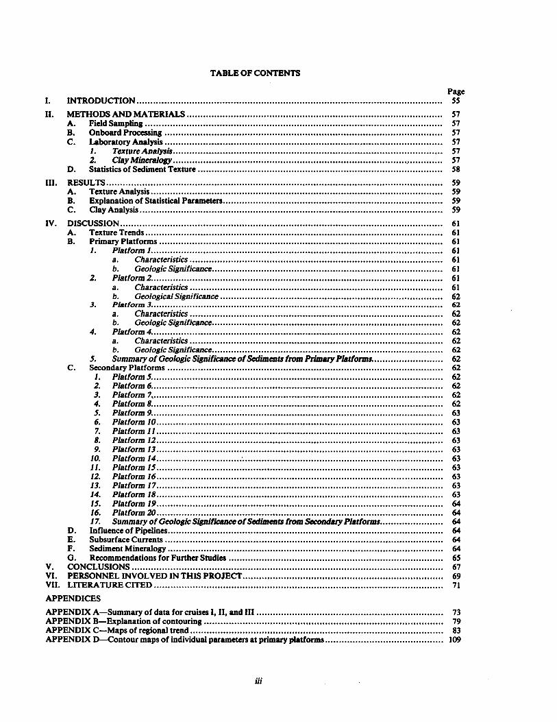
TABLE OF CONTENTS

Page I. INTRODUC'I'ION ... . . . . . . . . . . . . . . . . . . . . . . . . . . . . . . . . . . . . . . . . . . . . . . . . . . . . . . . . . . . . . . . . . . . . . . . . . . . . . . . . . . . . . . . . . . . . . . . . . . . . . . . . . . . . SS

II . METHODS AND MATERIALS .. . . . . . . . . . . . . . . . . . . . . . . . . . . . . . . . . . . . . . . . . . . . . . . . . . . . . . . . . . . . . . . . . . . . . . . . . . . . . . . . . . . . . . . . . . . . 57 A. Field Sampling ... . . . . . . . . . . . . . . . . . . . . . . . . . . . . . . . . . . . . . . . . . . . . . . . . . . . . . . . . . . . . . . . . . . . . . . . . . . . . . . . . . . . . . . . . . . . . . . . . . . . . . . . . . 57 B. Onboard Processing . . . . . . . . . . . . . . . . . . . . . . . . . . . . . . . . . . . . . . . . . . . . . . . . . . . . . . . . . . . . . . . . . . . . . . . . . . . . . . . . . . . . . . . . . . . . . . . . . . . . . 57 C. Laboratory Analysis . . . . . . . . . . . . . . . . . . . . . . . . . . . . . . . . . . . . . . . . . . . . . . . . . . . . . . . . . . . . . . . . . . . . . . . . . . . . . . . . . . . . . . . . . . . . . . . . . . . . . 57

1. Texture Analysis . . . . . . . . . . . . . . . . . . . . . . . . . . . . . . . . . . . . . . . . . . . . . . . . . . . . . . . . . . . . . . . . . . . . . . . . . . . . . . . . . . . . . . . . . . . . . . . . . . 57 2. CIayMineralogy . . . . . . . . . . . . . . . . . . . . . . . . . . . . . . . . . . . . . . . . . . . . . . . . . . . . . . . . . . . . . . . . . . . . . . . . . . . . . . . . . . . . ., . . . . . . . . . . . . 57

D. Statistics of Sediment Texture ... . . . . . . . . . . . . . . . . . . . . . . . . . . . . . . . . . . . . . . . . . . . . . . . . . . . . . . . . . . . . . . . . . . . . . . . . . . . . . . . . . . . . . . 58

III. RESUL'I'5 . . . . . . . . . . . . . . . . . . . . . . . . . . . . . . . . . . . . . . . . . . . . . . . . . . . . . . . . . . . . . . . . . . . . . . . . . . . . . . . . . . . . . . . . . . . . . . . . . . . . . . . . . . . . . . . . . . . . . . . . . . 59 A. Texture Analysis . . . . . . . . . . . . . . . . . . . . . . . . . . . . . . . . . . . . . . . . . . . . . . . . . . . . . . . . . . . . . . . . . . . . . . . . . . . . . . . . . . . . . . . . . . . . . . . . . . . . . . . . . . 59 B. Explanation of Statistical Paraaieters . . . . . . . . . . . . . . . . . . . . . . . . . . . . . . . . . . . . . . . . . . . . . . . . . . . . . . . . . . . . . . . . . . . . . . . . . . . . . . . . 59 C. Clay Analysis .. . . . . . . . . . . . . . . . . . . . . . . . . . . . . . . . . . . . . . . . . . . . . . . . . . . . . . . . . . . . . . . . . . . . . . . . . . . . . . . . . . . . . . . . . . . . . . . . . . . . . . . . . . . . . 59

IV . DISCUSSION . .. . . . . . . . . . . . . . . . . . . . . . . . . . . . . . . . . . . . . . . . . . . . . . . . . . . . . . . . . . . . . . . . . . . . . . . . . . . . . . . . . . . . . . . . . . . . . . . . . . . . . . . . . . . . . . . . . . . 61 A. Texture Trends . . . . . . . . . . . . . . . . . . . . . . . . . . . . . . . . . . . . . . . . . . . . . . . . . . . . . . . . . . . . . . . . . . . . . . . . . . . . . . . . . . . . . . . . . . . . . . . . . . . . . . . . . . . . 61 B. Primary Platforms . . . . . . . . . . . . . . . . . . . . . . . . . . . . . . . . . . . . . . . . . . . . . . . . . . . . . . . . . . . . . . . . . . . . . . . . . . . . . . . . . . . . . . . . . . . . . . . . . . . . . . . 61

1. Platform 1. . . . . . . . . . . . . . . . . . . . . . . . . . . . . . . . . . . . . . . . . . . . . . . . . . . . . . . . . . . . . . . . . . . . . . . . . . . . . . . . . . . . . . . . . . . . . . . . . . . . . . . . . . 61 a. Characteristics .. . . . . . . . . . . . . . . . . . . . . . . . . . . . . . . . . . . . . . . . . . . . . . . . . . . . . . . . . . . . . . . . . . . . . . . . . . . . . . . . . . . . . . . . . . . 61 b. Geologic Significance . . . . . . . . . . . . . . . . . . . . . . . . . . . . . . . . . . . . . . . . . . . . . . . . . . . . . . . . . . . . . . . . . . . . . . . . . . . . . . . . . . . . 61

2. Platform 2. . . . . . . . . . . . . . . . . . . . . . . . . . . . . . . . . . . . . . . . . . . . . . . . . . . . . . . . . . . . . . . . . . . . . . . . . . . . . . . . . . . . . . . . . . . . . . . . . . . . . . . . . . 61 a. Characteristics .. . . . . . . . . . . . . . . . . . . . . . . . . . . . . . . . . . . . . . . . . . . . . . . . . . . . . . . . . . . . . . . . . . . . . . . . . . . . . . . . . . . . . . . . . . . 61 6. Geological Significance . . . . . . . . . . . . . . . . . . . . . . . . . . . . . . . . . . . . . . . . . . . . . . . . . . . . . . . . . . . . . . . . . . . . . . . . . . . . . . . . . 62

3. Platform 3. . . . . . . . . . . . . . . . . . . . . . . . . . . . . . . . . . . . . . . . . . . . . . . . . . . . . . . . . . . . . . . . . . . . . . . . . . . . . . . . . . . . . . . . . . . . . . . . . . . . . . . . . . 62 a. Characteristics .. . . . . . . . . . . . . . . . . . . . . . . . . . . . . . . . . . . . . . . . . . . . . . . . . . . . . . . . . . . . . . . . . . . . . . . . . . . . . . . . . . . . . . . . . . . 62 b. Geologic Significance . . . . . . . . . . . . . . . . . . . . . . . . . . . . . . . . . . . . . . . . . . . . . . . . . . . . . . . . . . . . . . . . . . . . . . . . . . . . . . . . . . . . 62

4. Platform 4. . . . . . . . . . . . . . . . . . . . . . . . . . . . . . . . . . . . . . . . . . . . . . . . . . . . . . . . . . . . . . . . . . . . . . . . . . . . . . . . . . . . . . . . . . . . . . . . . . . . . . . . . . 62 a . Characteristics . . . . . . . . . . . . . . . . . . . . . . . . . . . . . . . . . . . . . . . . . . . . . . . . . . . . . .. . . . . . . . . . . . . . . . . . . . . . . . . . . . . . . . . . . . . . 62 b. Geologic Significance . . . . . . . . . . . . . . . . . . . . . . . . . . . . . . . . . . . . . . . . . . . . . . . . . . . . . . . . . . . . . . . . . . . . . . . . . . . . . . . . . . . . 62

S. Summary of Geologic Sigtificance of Sediments from Primary Platforms. . . . . . . . . . . . . . . . . . . . . . . . . . 62 C . Secondary Platforms . . . . . . . . . . . . . . . . . . . . . . . . . . . . . . . . . . . . . . . . . . . . . . . . . . . . . . . . . . . . . . . . . . . . . . . . . . . . . . . . . . . . . . . . . . . . . . . . . . . . 62

1 . Platform 5. . . . . . . . . . . . . . . . . . . . . . . . . . . . . . . . . . . . . . . . . . . . . . . . . . . . . . . . . . . . . . . . . . . . . . . . . . . . . . . . . . . . . . . . . . . . . . . . . . . . . . . . . . 62 2. Platform 6. . . . . . . . . . . . . . . . . . . . . . . . . . . . . . . . . . . . . . . . . . . . . . . . . . . . . . . . . . . . . . . . . . . . . . . . . . . . . . . . . . . . . . . . . . . . . . . . . . . . . . . . . . 62 3 . Platform 7. . . . . . . . . . . . . . . . . . . . . . . . . . . . . . . . . . . . . . . . . . . . . . . . . . . . . . . . . . . . . . . . . . . . . . . . . . . . . . . . . . . . . . . . . . . . . . . . . . . . . . . . . . 62 4 . Platform 8. . . . . . . . . . . . . . . . . . . . . . . . . . . . . . . . . . . . . . . . . . . . . . . . . . . . . . . . . . . . . . . . . . . . . . . . . . . . . . . . . . . . . . . . . . . . . . . . . . . . . . . . . . 62 S. Platform 9. . . . . . . . . . . . . . . . . . . . . . . . . . . . . . . . . . . . . . . . . . . . . . . . . . . . . . . . . . . . . . . . . . . . . . . . . . . . . . . . . . . . . . . . . . . . . . . . . . . . . . . . . . 63 6. Platform 10 . . . . . . . . . . . . . . . . . . . . . . . . . . . . . . . . . . . . . . . . . . . . . . . . . . . . . . . . . . . . . . . . . . . . . . . . . . . . . . . . . . . . . . . . . . . . . . . . . . . . . . . . 63 7. Platform I1 . . . . . . . . . . . . . . . . . . . . . . . . . . . . . . . . . . . . . . . . . . . . . . . . . . . . . . . . . . . . . . . . . . . . . . . . . . . . . . . . . . . . . . . . . . . . . . . . . . . . . . . . 63 8. Platform 12 . . . . . . . . . . . . . . . . . . . . . . . . . . . . . . . . . . . . . . . . . . . . . . . . . . . . . . . . . . . . . . . . . . . . . . . . . . . . . . . . . . . . . . . . . . . . . . . . . . . . . . . . 63 9. Platform 13 . . . . . . . . . . . . . . . . . . . . . . . . . . . . . . . . . . . . . . . . . . . . . . . . . . . . . . . . . . . . . . . . . . . . . . . . . . . . . . . . . . . . . . . . . . . . . . . . . . . . . . . . 63 10. Platform 14 . . . . . . . . . . . . . . . . . . . . . . . . . . . . . . .: . . . . . . . . . . . . . . . . . . . . . . . . . . . . . . . . . ., . . . . . . . . . . . . . . . . . . . . . . . . . . . . . . . . . . . . . 63 11 . Platform 15 . . . . . . . . . . . . . . . . . . . . . . . . . . . . . . . . . . . . . . . . . . . . . . . . . . . . . . . . . . . . . . . . . ., . . . . . . . . . . . . . . . . . . . . . . . . . . . . . . . . . . . . . 63 12. Platform 16 . . . . . . . . . . . . . . . . . . . . . . . . . . . . . . . . . . . . . . . . . . . . . . . . . . . . . . . . . . . . . . . . . ., . . . . . . . . . . . . . . . . . . . . . . . . . . . . . . . . . . . . . 63 13. Platform 17 . . . . . . . . . . . . . . . . . . . . . . . . . . . . . . . . . . . . . . . . . . . . . . . . . . . . . . . . . . . . . . . . . . . . . . . . . . . . . . . . . . . . . . . . . . . . . . . . . . . . . . . . 63 14. Platform 18 . . . . . . . . . . . . . . . . . . . . . . . . . . . . . . . . . . . . . . . . . . . . . . . . . . . . . . . . . . . . . . . . . ., . . . . . . . . . . . . . . . . . . . . . . . . . . . . . . . . . . . . . 63 15. Platform 19 . . . . . . . . . . . . . . . . . . . . . . . . . . . . . . . . . . . . . . . . . . . . . . . . . . . . . . . . . . . . . . . . . ., . . . . . . . . . . . . . . . . . . . . . . . . . . . . . . . . . . . . . 64 16. Platform 20. . . . . . . . . . . . . . . . . . . . . . . . . . . . . . . . . . . . . . . . . . . . . . . . . . . . . . . . . . . . . . . . . . . . . . . . . . . . . . . . . . . . . . . . . . . . . . . . . . . . . . . . 64 17. Summary of Geologic Significance of Sediments from Secondary Platforms. . . . . . . . . . . . . . . . . . . . . . . 64

D. Influence of Pipelines.. . . . . . . . . . . . . . . . . . . . . . . . . . . . . . . . . . . . . . . . . . . . . . . . . . . . . . . . . . . . . . . . . . . . . . . . . . . . . . . . . . . . . . . . . . . . . . . . . . . 64 E. Subsurface Currents .. . . . . . . . . . . . . . . . . . . . . . . . . . . . . . . . . . . . . . . . . . . . . . . . . . . . . . . . . . . . . ., . . . . . . . . . . . . . . . . . . . . . . . . . . . . . . . . . . . . . 64 F. Sediment Mineralogy ... . . . . . . . . . . . . . . . . . . . . . . . . . . . . . . . . . . . . . . . . . . . . . . . . . . . . . . . . . . . . . . . . . . . . . . . . . . . . . . . . . . . . . . . . . . . . . . . . . 64 G. Recommendations for Further Studies .. . . . . . . . . . . . . . . . . . . . . . . . . . . . . . . . . . . . . . . . . . . . . . . . . . . . . . . . . . . . . . . . . . . . . . . . . . . . . 65

V. CONCLUSIONS . . . . . . . . . . . . . . . . . . . . . . . . . . . . . . . . . . . . . . . . . . . . . . . . . . . . . . . . . . . . . . . . . . . . . . . . . . ., . . . . . . . . . . . . . . . . . . . . . . . . . . . . . . . . . . . . . 67 VI . PERSONNEL INVOLVED IN THIS PROJECT... . . . . . . . . . . . . . . . . . . . . . . . . . . . . . . . .» . . . . . . . . . . . . . . . . . . . . . . . . . . . . . . . . . . . . . 69 VII. LITERATURE CITED ... . . . . . . . . . . . . . . . . . . . . . . . . . . . . . . . . . . . . . . . . . . . . . . . . . . . . . . . . . . . . . . . . . . . . . . . . . . . . . . . . . . . . . . . . . . . . . . . . . . . . . . 71

APPENDICES

APPENDIX A-Summary of data for cruises I, II, and III . . . . . . . . . . . . . . . . . . . . . . . . . . . . . ., . . . . . . . . . . . . . . . . . . . . . . . . . . . . . . . . . . . . . 73 APPENDIX B-Explanation of contouring ... . . . . . . . . . . . . . . . . . . . . . . . . . . . . . . . . . . . . . . . . . . . . . . . . . . . . . . . . . . . . . . . . . . . . . . . . . . . . . . . . . . . . 79 APPENDIX C-Maps of regional trend . . . . . . . . . . . . . . . . . . . . . . . . . . . . . . . . . . . . . . . . . . . . . . . . . . . . . ., . . . . . . . . . . . . . . . . . . . . . . . . . . . . . . . . . . . . . 83 APPENDIX D-Contour maps of individual parameters at primary platforms ... . ., . . . . . . . . . . . . . . . . . . . . . . . . . . . . . . . . . . . . . 109

iii

ABSTRACT

The sediment texture for 1,668 samples and sediment mineralogy for 56 samples have ban analyzed . Sediments collected from most platforms are fine to medium grained silts and are poorly to very poorly sorted. At all platforms, smectite is the most abundant clay mineral and may play a significant role is the chemistry of water, sediments, and organisms because of its unique absorption-exchange properties .

I . INTRODUCTION

Sea floor sediment texture and mineralogy are extremely important variables in the evaluation of environmental impacts due to petroleum exploration and production activities . The relative proportions of sand, silt, and clay sized material play an important role in infaunal community population size and dynamics (Harper, 1977) . In addition, trace ion and hydrocarbon accumulation has been shown to be sediment depen-dent . Fine grained clay minerals, which comprise a significant amount of surface sediments, are believed to transport chemical and biological constituents and pollutants by adsorption, complexing, and/or exchange at the clay-water interface . Moreover, clays act as "competitors" with organisms (particularly benthos) for uptake of certain chemical constituents and pollutants at the clay-water-organism interface in which a dynamic equilibrium is being continuously main-tained . A number of authors (Ruch, Kennedy, and Shimp, 1970 ; Leland, Shukla, and Shimp, 1973 ; Hildebrand and Blum, 1974 ; Catazaro, 1976 ; Scrudato

and Estes, 1976) have partially delineated the relationships between trace ions and clay minerals relative to sorption processes occurring under various environmental conditions . Additional work (Shimp, Leland, and White, 1970) has shown that an inter-relationship exists between sediment type, trace ion in-take, and the concentration of these contaminants by benthic organisms . Studies in Sarosota Bay, Tampa Bay (Huang, 1975, 1976) and the MAFLA area (Huang, 1976) have also shown the existence of such interrelationships .

The purpose of this report is to (1) delineate sediment textural characteristics, assess variances noted in both time and space at 20 platforms and 4 control sites, and provide a basis for correlation of chemical contami-nants, microbial ecology and benthic organisms with the sediment type ; and to (2) characterize clay and carbonate minerals of surface sediments from 20 platforms and 4 control sites for possible assessment of their relationships with other parameters .

55

II . METHODS AND MATERIALS

A. Field Sampling A Kahlsico (No . 214WA250) stainless steel, mod-

ified Smith-McIntyre grab (Smith and McIntyre, 1954) was used to collect sediments for texture analysis and mineralogy . The grab sampled an area of 0.1 m2 to a depth of 12-15 cm. Depth of penetration varied with sediment type . Most of the sediments in the area under study are fine-grained ; therefore, the Smith-McIntyre grab usually penetrated to its maximum depth, and al-ways sufficiently to allow consistent subsampling .

A total of 1,668 samples were collected for sediment texture analysis . These include 488 samples collected during Cruise I, May, 1978; 806 samples (plus 14 dupli-cates) collected during Cruise II, August and Septem-ber, 1978 ; and 360 samples collected during Cruise III, January, 1979 . A texture analysis sample was taken from every grab taken . This allowed for the evaluation of seasonal sediment changes at Primary Platforms and Control Sites .

Samples for analysis of clay and carbonate mineral-ogy were collected once from each study site according to the following table :

Station Locations Total Number

Primary Platforms (4) N500 20 N2A00 E2000 52000 W2000

Secondary Platforms (16) N500 32 N2000

Control Sites (4) NA 4 56

B. Onboard Processing A 5 cm diameter x 5 cm deep (minimum 100 g) sub-

core was taken from each of the 1,668 grabs for sedi-ment characterization . Thus, a constant sample volume was removed from each grab . Each sample was placed in a plastic bag, labeled, inventoried and stored in ship-ping containers . When samples reached the laboratory at the end of the cruise, standard procedures of sample inventory and reporting to data management were fol-lowed .

C. Laboratory Analysis

i. Texture Analysis Each sample was homogenized, air dried, and

approximately 70 g were weighed and treated with an al-iquot of 10% hydrogen peroxide (HZOZ) to oxidize or-ganic matter . The remaining material was retained for any subsequent analyses necessary . Soluble salts were removed by washing twice with distilled water . The sam-ple was then oven dried at 100 C for 12 hours . A mini-mum of 2 hours was allowed for equilibration to am-bient laboratory conditions . The sample was wet sieved using a 0.0625-mm mesh to separate the sand from the silt-clay fraction . The sand and greater size fraction was dried at 100 C for 12 hours, then sieved at 1/2 phi inter-vals (-1 .0, -0 .5, 0.1, 0.5, 1 .0, 1 .5, 2 .0, 2.5, 3 .0, 3 .5, 4.0) .

Each collected fraction was examined for aggregates, disaggregated if necessary, and reweighed by fraction to three significant numbers . The silt-clay fraction was analyzed for particle size distribution by the pipette (set-tling rate) method at 4.0, 5 .0, 6 .0, 7 .0, 8 .0, 9 .0, 10.0 and >10.0 phi intervals . Individual percent and cumulative percent were calculated for each fraction and stored on computer tapes . A data summary for sediment analysis is given in Volume :[, Part 8 .

The analytical procedure that is followed in de-termining the texture of sediments may, in itself, alter the texture of the sediments and lead to spurious results . In this study, washing with distilled water essentially changed the interstitial condition of the sediment from marine to fresh water, and may have reversed the flocu-lation that occurred as the clay minerals were carried from the Mississippi River into the Gulf of Mexico . Thus, the particle size may have been reduced . On the other hand, oven drying may have formed larger parti-cles than those of the sediment as deposited . Sedimento-logists are not able to specify an analytical procedure which will avoid pitfalls such as these . The procedure followed in this study is standard and was applied uni-formly to all samples . Thus, any errors introduced should not obscure textural trends either regionally or locally around individual platforms .

2. Clay Mineralogy For clay mineralogy, each sediment was digested

in deionized water overnight to insure complete dispers-ion. The clay fractions (<21A) were completely separated from the bulk sample by treating with 1 ml of 2.5 M NH40H (dispersing agent) prior to centrifuging for 2 minutes at 1000 RPM. Two oriented clay slides were prepared for each sample by treatment with Mg-Glycer-ated saturation and K-saturation . To minimize any ex-perimental variation in the estimate of relative percent-ages of individual clay minerals, a 35-#A clay film was prepared on ceramic tiles for X-ray diffraction analysis . For each sample at least eight separate X-ray diffraction analyses, followed by different treatments and heating, were made in order to identify all major types of clay minerals and to estimate semiquantitatively the relative percentage of each clay mineral in the sample . Identifi-cation of the 141 chlorite-vermiculite mixed layers, which is also unique in the west Florida shelf for the MAFLA program, follows the criteria discussed by Huang, Larry, and Chiou (1975) .

The relative percentage of clay minerals was de-termined on a semiquantitative basis, following the technique of Huang et al . (1975) modified after Carroll (1970) and other :; . The refinement of the estimate has been made through the standardization of the sample preparation, treatment and the X-ray diffraction, the consideration of mass-absorption coefficient of miner-als, and the calibration with known amounts of stan-dard clay samples . The determination was based on the measurement of the (001) peak area (at least three times by a planimeter;), from the Mg-glycerol samples for smectite, chlorite, chlorite-vermiculite, kaolinite, and from the K-saturated samples for illite . The chlorite and kaolinite were also estimated by comparing the

57

intensities of 3 .58A (002 for kaolinite) and 3 .54A (004 for chlorite). Other clay and non-clay minerals were es-timated using the most intensive hkl peaks after cali-bration with known amounts of standard samples pre-pared with the same procedure. Techniques which were used for the 1974-1976 MAFLA projects, eastern Atlan-tic continental slope, and Tampa Bay projects have been used for this project.

Carbonate and bulk mineralogy in both the finer clay fractions (<2N) and bulk sediments were deter-mined by X-ray diffraction analysis and compared qual-itatively and semi-quantitatively to determine if any sig-nificant variations of major carbonate minerals (arago-nite, low-Mg calcite, dolomite) and other non-clay minerals existed among stations .

D. Statistics of Sediment Texture To determine geologic significance of sediment tex-

ture in the study area, the following statistical parame-ters were computed . They are standard measures of sed-iment analysis and are thoroughly described in any in-troductory sedimentology text .

a . Percentage of sand, silt, and clay b . Measure of average size

(1) Median (Md) _ 050 (2) Graphic Mean (Mz) _ (mob + (050 + 089)/3

c. Measure of Uniformity (sorting) Inclusive graphic standard deviation

(°d _ 084 4 0'6+1.a4) Verbal scale of sorting

d . Measure of Skewness or Asymmetry Inclusive graphic Skewness

SK = X16 + X84 - 2050 + '*s + 495 - 2 50

2 N'gy - O1d

e . Measure of Kurtosis or Peakedness Graphic Kurtosis

KG = 4095 - 05 2.44 (4075 - 4)25)

58

III . RESULTS

A. Texture Analysis Statistical data for each sample site calculated by the

techniques discussed above were stored on computer tape . Summaries of data are tabulated in Appendix A. Criteria used in preparing contour maps from these summaries are explained in Appendix B . Data were plotted and contoured on maps for the entire study area (Appendix C) and for individual Primary Platforms (P1-4) (Appendix D) . Since Secondary Platforms (SS-20) were sampled during only one season at four loca-tions on a north transect, their data were not contoured .

For each individual Primary Platform, a contour map was made for each grain size . A total of 84 contour maps were made and were used to define the general current direction and flow regime for each area .

Average percentages for each grain size from each site were calculated and contoured on the regional maps. Thus three regional contour maps per cruise were made, showing the general distribution of sand, silt, and clay . These nine contour maps provide information on the influence of rivers and the general distribution of their load . These were compared to the hydrography data and maps .

B. Explanation of Statistical Parameters

1 . Standard Deviation-the degree to which the sed-iment is sorted . A small value for standard devia-tion indicates that a narrow range of grain size is present and that the sediment is well sorted . A large value, conversely, indicates that a wide range of grain size is present and that the sedi-ment is poorly sorted . A range of grain sizes in a sediment may reflect multiple sources, and thus potentially local contamination of the natural sediment by addition of material derived from some operation at the platform site . On the other hand, a range of sizes may reflect variations in water energy in the natural environment as sedi-ment is transported, eroded and deposited under different conditions of wave and current action . The sediment deposited during these different pe-riods will of course be thoroughly mixed by orga-nisms living on the sea floor .

2. Kurtosis-the peakedness of the size frequency distribution curve. It indicates the extent to which the sediment is predominantly of a narrow size

range . It does not reflect as strongly as does stan-dard deviation the total range of sizes within the sediment . If a large fraction of the sediment falls within a narrow size range and only a small frac-tion is in the very small or very large size classes, the kurtosis will be high - the sediment is lepto-kurtic . Conversely, in a platykurtic sediment, par-ticle size is not strongly clustered around a domi-nant value but is more widely distributed . The general interpretation of kurtosis is similar to that of standard deviation. It indicates multiple sources of sediment and/or variations in the de-position regime . Skewness-the degree to which and direction in which the grain size distribution is skewed . A sample with equal proportions of fine and coarse material on either side of the mean size will have a normal or bell shaped size distribution curve, and a skewness of zero . A sample with a predomi-nance of grains coarser than the mean size will have a high positive skewness value . A sample containing a predominance of grains smaller than a mean size will have a large negative value . The skewness value indicates whether the sediment is predominantly coarse with an added mixture of fines or fine grains with an added mixture of coarse grains. Its general interpretation might in-dicate whether the sediment has been contami-nated . A high or low value of skewness may sug-gest that the predominant texture of the sediment has been modified by an admixture potentially through contamination of sediment that is differ-ent from that which would normally occur .

C. Clay Analysis Results of clay analysis of sea floor sediments (<2-#A

fractions) are shown in Appendix A, Tables A4 and AS for Cruise I and II, respectively . Tables A6 and A7 show the results of analysis of bulk minerals (including car-bonate minerals) in the sediments ; percentage of each specific clay mineral in bulk sediments (instead of <2-IA fractions only) was calculated and is shown in these tables .

Total clay content ranges from less than 10% to more than 40% of the total sediment . Smectite is the dominant clay mineral in all samples, with only illite and kaolinite present as significant accessory clay minerals .

59

IV . DISCUSSION

A. Texture Trends Appendix C contains area maps charting contours

of the parameters measured for all stations over three cruises .

In general, the percentage of sand decreases with in-crease in silt percentage seaward from the shore with the following exceptions . (a) In the area around Secondary Platforms 519, S11 and P3 there appears to be an in-crease in sand and a decrease in silt. Platform S19 is lo-cated on Ship Shoal, a prominent sandy shoal which emerges 4-6 m above the surrounding silty floor . (b) In the area close to the shore south-southwest of Timbalier Bay and Barataria Bay a high percentage of silt and clay was found . This is an area which apparently has re-ceived substantially less direct flow from the Mississippi in past geologic time, and is in the pocket of isolated oceanic water cut off by the present day major distribu-tary delta. The predominant clay mineral is smectite. (c) Near shore, there is a trend toward increase in total clay content and smectite, particularly west of the Missis-sippi and south of Barataria Bay . This suggests that a large portion of clay is brought in by the Mississippi and is flocculated after entering the Gulf . It is conceivable that the relatively low energy of the longshore current carries and transports the relatively fine particles along the shore . The standard deviation of samples collected in most of the area indicates the sediments are poorly to very poorly sorted . This is to be expected because of the predominant silt size . However, sediments from Plat-form S19 are better sorted because of the relative abun-dance of sand .

With respect to skewness and kurtosis, sediments appear to be more strong-fine skewed and leptokurtic seaward from the shore . This suggests that there is a ten-dency for the average grain size to move further from the mean and be more grouped around the finer grain size .

B. Primary Platforms The general trend exhibited appears to be one in

which there is an accumulation of coarse material around the platform and more to one side than the other . This polarized distribution pattern appears to be attributed to decreasing current speed through the phys-ical barrier of the platform, causing the deposition of coarse material on one side and around the platform . As the current moves past the platform at a slower speed the finer materials, or silt and clay, are deposited mostly on the other side and further away from the platform . It should be pointed out, however, that some exceptions are observed and are presumably attributed to the direc-tion of the prevailing current at the time.

Primary Platforms discussed in the following section are graphically described sequentially in Appendix D. These graphs plot and contour percentage sand, silt and clay, means, standard deviations, skewness and kurto-sis, respectively, for each site and each of three cruises .

1. Platform 1

a. Characteristics Platform 1 (P1) shows a marked higher per-

centage of sand on the north-northeast side of the

platform in Cruise I, with the expected decrease in silt and clay . However, this is not as evident in Cruises II and III . The percentage of sand in Cruises II and III tends toward an increase outward from the platform, and an increase toward the east . The graphic mean of grain size also indicates the sand trend.

Cruise I shows a higher standard deviation in the eastern half of the map area . In Cruises II and III, sorting (standard deviation) increases in all directions outward from the platform . Cruise III shows a higher standard deviation in the WNW quadrant . Sediments from all cruises show poor to very poor sorting .

Sediments from all three cruises indicate skewness becoming more strong, i .e ., fine, outward from the platform, particularly to the west of the plat-form . Skewness also becomes nearly symmetrical on the WNW side of the platform and toward the center in Cruises I and II .

Cruise I sediments change from primarily mesokurtic in the west to leptokurtic in the east . Cruise II shows them to be primarily mesokurtic becoming more leptokurtic .Cruise III shows them to be primarily platykurtic becoming very platykurtic toward the center and to the east.

6. Geologic Significance In the spring of 1978 large amounts of sedi-

ment were being transported from the Mississippi River westward by a high-energy longshore current . This long-shore current appears to have become significantly less intense by the end of the summer as well as in mid-win-ter . Thus, in the spring, during seasonal high discharge, transportation of sediment is at its greatest . By the sum-mer, river discharge has subsided and less coarse sedi-ment is being brought into the Gulf of Mexico . Compa-rison of the maps for Platform 1 at different times indi-cates that deposition at the platform is affected by this seasonal pattern of sediment influx . Coarse grains are deposited near the platform and surrounding it during the spring . Percentages of sand in the spring are as much as 21 % greater than in the other two sampling pe-riods . Discharge of the Mississippi River during the spring of 1978 was much greater than during the follow-ing late summer and mid-winter, being almost three times greater during April than in August 1978 . This higher rate of flow obviously carried greater amounts of coarser sediment .

2. Platform 2

a . Characteristics There as a shifting from a high percentage of

sand to the ENE of P2 in Cruise I to a more even distri-bution around the platform in Cruise II to a higher per-centage of sand to the SSE in Cruise III . The clay frac-tion increases steadily to the westward on all cruises . The graphic mean also shows the increase of fine grains westward in all cruises .

There is an increase in standard deviation outward from the platform in all cruises . Skewness of sediments in all three cruises shows a trend from strong-fine to strong-coarse from NE to NW. However, in

61

general, skewness is particularly strong-fine in the ESE center around the platform .

All three cruises show a trend toward more platykurtic sediments toward the west . Cruises I and II show very leptokurtic sediments in the center, to the east of the platform .

b. Geological Significance At this platform, current direction in the

winter seems to shift from that in the spring or summer, that is, from the northeast to the southeast . The change is presumably due to the decrease in discharge from the Mississippi River and thus greater influence of ocean currents to the platform .

3. Platform 3

a. Characteristics All three cruises show marked increase in

percent sand toward the North . However, in Cruise III the percentage of sand seems higher in the NNW as compared to the NNE in Cruise I . In Cruise I, sand is also concentrated around the platform . The graphic mean also shows a similar pattern .

There is an increase in the standard deviation from north to south in all three cruises . Furthermore, all cruises show a change from poorly sorted to very poorly sorted sediments from the north to the south, and in general sediments are better sorted in the center around the platform .

The skewness of sediments in Cruise I is strong-fine in the center and becomes coarse-skewed to the NNE and SSE . Cruise II skewness tends toward fine in the south, whereas in Cruise III it becomes more coarse toward the NNW and WSW.

Sediments from Cruises I and III show a trend toward very leptokurtic to platykurtic kurtosis from north to south, but sediments from Cruise II are very leptokurtic to platykurtic from ENE to WSW, to very leptokurtic in the ENE .

6. Geologic Significance The current at Platform 3 appears to be un-

affected by the seasons because of its position . The geo-logic influence of river discharges is relatively small .

4. Platform 4

a. Characteristics In general, all cruises show a higher concen-

tration of sand NNW of the platform . Sediments also have a much higher concentration of sand around the platform in Cruise I than in Cruises II and III . The dis-tribution of silt and clay follows closely that of the sand and shows higher percentages further from the platform to the west and south . The graphic mean shows an in-crease of fine materials outward from the platform in all cruises .

In Cruises I and II standard deviation in-creases northward indicating a more poor sorting. How-ever, Cruise III shows an increase in sorting N and SSW.

Skewness of sediments in Cruises I and II shows a trend from fine to coarse toward P4 . However, Cruise III shows the trend to be strong-fine skewed to strong-coarse skewed from ESE to WNW .

Cruise I showed kurtosis to be more platy-kurtic in the NNW to very leptokurtic from N to S. Kur-tosis in Cruise III shows a change from very platykurtic to leptokurtic from ESE to WNW .

b. Geologic Significance Platform 4 shows little seasonal current

change and a large percentage of fines, whereas nearby Platform 3 shows a much higher percentage (70%) of sand .

S. Summary of Geologic Significance of Sediments from Primary Platforms Platforms 1 and 2 show the significant effect of

the longshore current on the distribution of sediments because of the platforms' close proximity to shore . Plat-form 4, far out to sea, shows a large amount of fines uniformly distributed as expected . However, P3, which is also away from the shore, shows a significant percent-age of sand and coarse materials rather than fines . The high concentration of sands at P3 may result from the interaction of two currents : the longshore current and possibly the Gulf's loop current . The sediment after being ejected into the Gulf by rivers is carried westward, close to shore, by the longshore current . As it moves west, it encounters a landform just west of Barataria Bay, and is forced to the southwest, deeper into the Gulf . Just south of Timbalier Bay, it resumes its west-ward movement, and encounters the Gulf's loop cur-rent, which is moving eastward . The longshore current loses its speed and drops most of its coarse material in the area .

C. Secondary Platforms

1. Platform S Sand increases and silt and clay decrease toward

the platform . Mean grain size shows a decrease in the phi size . Sediments are generally more poorly sorted to-ward the platform . Skewness becomes finer toward the platform and kurtosis becomes more leptokurtic toward the platform .

2. Platform 6 No definite trends of sand, silt, and clay distribu-

tion are observed because of relatively few samples available . The graphic mean shows that fine sediments are concentrated toward the platform . Standard devia-tion increases toward the platform . Skewness trends from nearly symmetrical to coarsely skewed toward the platform . Kurtosis grades from platykurtic to leptokur-tic toward the platform .

3. Platform 7 Fine sediment increases away from the platform,

particularly at about 500 m from the platform . Stan-dard deviation is also high at 500 m from the platform, indicating very poor sorting there . Skewness trends to-ward strong coarse skewed toward the platform . The kurtosis is leptokurtic toward the platform .

4. Platform 8 Sand percentage and the graphic mean both in-

crease toward the platform . Sediment sorting is very poor near the platform . The skewness is finely skewed near the platform grading to strong-fine skewed

62

outward. Kurtosis is platykurtic to very platykurtic near the platform .

S. Platform 9 Sand percentage and graphic mean increase to-

ward the platform, whereas the percentages of silt and clay increase outward from the platform with the lowest silt percentage and highest clay percentage at the S00-m station . Sorting is better outward from the platform but remains relatively poor throughout the area . Skewness ranges from near symmetrical near the platform to fine-skewed outward from the platform . Sediments are gen-erally leptokurtic and become very leptokurtic at the 1000-m station .

6. Platform 10 Sand percentage increases outward from the

platform but graphic mean and percentages of silt and clay increase toward the platform . Sediments are gener-ally poorly sorted but become better sorted toward the platform . The skewness is generally strong-fine skewed, but becomes strong-coarse skewed at the 1000-m sta-tion . Sediments are very platykurtic throughout the area .

7. Platform 11 Sand percentage increases toward the platform,

whereas the percentage of silt decreases . The percentage of clay remains relatively constant throughout the area . The graphic mean indicates that coarser material in-creases in abundance toward the platform . Based on standard deviation data, the sediments in the area are poorly sorted, becoming more poorly sorted toward the platform . Skewness is strong-fine skewed throughout the area but approaching the platform become fine skewed . Kurtosis changes from very platykurtic to lep-tokurtic toward the platform .

8. Platform 12 Sand percentage decreases toward the platform .

Silt percentage also decreases and clay increases toward the platform . Silt is abnormally abundant and clay and sand are rare at the 1000-m station . The graphic mean indicates a fining inward toward the platform with more silt in the area of the 1000-m station . Standard deviation indicates that the sediments are poorly sorted through-out the area, but somewhat better sorted in the area of 500 to 1000 m . Skewness ranges from near-symmetrical to strong-fine skewed outward . Kurtosis grades from platykurtic to mesokurtic toward the platform, but sedi-ments from 500 to 1000 m are very leptokurtic .

9. Platform 13 Sand percentage increases inward toward the

platform . Silt percentage also increases inward with an abnormally high percentage at the 500-m station . Clay decreases inward . The graphic mean also indicates sedi-ment becomes finer toward the platform . Sediments are generally poorly sorted but become better sorted toward the platform . The skewness becomes more strong-fine skewed toward the platform . Sediments are very platy-kurtic to mesokurtic away from the platform but the sample from the 1000-m station is leptokurtic .

10. Platform 14 Sand percentage increases toward the platform,

particularly rapidly near the platform . Silt and clay

percentages decrease toward the platform from high concentrations in the area of 500 to 1000 m . The graphic mean shows this coarsening trend toward the platform . The sediments are poorly sorted grading to very poorly sorted toward the platform . In the area of the 1000-m station, the sediments are moderately sorted . Skewness grades from strong-fine skewed at the 1000-m station to coarse skewed away from the 1000-m station . The kur-tosis shows the same trend, ranging from platykurtic at the 1000-m station to leptokurtic .

11 . Platform 15 Sand percentage increases toward the platform

with a small decrease at the 500-m station . Silt percent-ages decrease inward toward the platform with the ex-ception of an increase at the 500-m station . The percent-age of clay decreases between the 2000- and 1000-m sta-tions and remains constant from the 1000-m station to the platform . The graphic mean also shows the coarsen-ing trend toward the platform . Sediment sorting changes from moderately-well sorted inward to poorly sorted . Kurtosis changes from very platykurtic to very leptokurtic inward, but the sample at the 500-m station is abnormally mesokurtic as compared to those from the 1000 and 100-m stations .

12 . Platform 16 Sand percentage decreases toward the platform

with an abnormally low percentage at the 500-m station . Silt percentage increases and clay percentage decreases inward . Percent silt is exceptionally low and percent clay high at the 500-m station . The graphic mean indi-cates a coarsening trend toward the platform except for the finer grain size at the 500-m station . The sediments range from well sorted to poorly sorted outward from the platform except that they are more poorly sorted at the 500-m station than at the 1000-m station . Skewness grades from strong-fine skewed at 100 m to fine skewed at the 2000-m station but are anomalously fine skewed at the 500-m station . Kurtosis ranges from very platy-kurtic to leptokurtic outward from the platform, with sediments at the 500-m station being more leptokurtic than the 2000-m station .

13 . Platform 17 Sand increases and silt decreases toward the

platform except at the 100-m station, where sand per-centage is lower and clay percentage is higher than ex-pected . The graphic mean also reflects this general coar-sening trend inward . Standard deviation indicates that the sediments grade from moderately sorted inward to very poorly sorted . Skewness ranges from coarse-skewed at the platform outward to strong-fine skewed . Kurtosis grades From very platykurtic inward to very leptokurtic .

14. Platform 18 Sand percentage generally increases and silt per-

centage decreases toward the platform . However, the sample from the 1000-m station has a high concentra-tion of clay, and the graphic mean indicates a fining in-ward with the maximum around the 1000-m station, The sediments grade from poorly sorted inward to very poorly sorted . Skewness grades from near symmetrical at the platform outward to strong-fine symmetrical . Kurtosis grades from leptokurtic outward to very platykurtic .

63

IS. Platform 19 Sand percentage is relatively high near the plat-

form . The graphic mean shows the same trend of in-creasing coarseness toward the platform . Standard devi-ation data indicates that the sediments are very well sorted throughout the area . Skewness ranges from nearly symmetrical to coarse skewed toward the plat-form . Kurtosis ranges from mesokurtic outward to very leptokurtic . Area maps indicate the large sandy shoal known as "ship shoal ." This explains the large amounts of coarse material and the very leptokurtic kurtosis .

16. Platform 20 Sand percentage decreases away from the 500-

m station along with a corresponding increase in silt and clay . The graphic mean also decreases away from the 500-m station . The sediments are very poorly sorted . Skewness ranges from strong-fine skewed at the 500-m station to fine skewed away from it . Kurtosis follows the same pattern, being less mesokurtic and more platy-kurtic outward .

17. Summery of Geologic Significance of Sedi-ments from Secondary Platforms The data show an increase in the percentage of

sand inward toward the platform for more than half of the secondary platforms . This is probably due to the structure acting as a barrier, thus causing the current to slow down and deposit sand . Platform S12 shows a gen-eral decrease in silt with an increase at 1000 m, whereas S16 shows a decrease in clay with an increase at the 500-m station .

Sediments from all secondary platforms are generally very poorly sorted, as expected, because most of the sediments are in the silt size . Exceptions are those from platforms where sands are predominant, and gen-erally sediments are medium-well sorted because of transportation and eddy current sweeping sand from the beach onto the platform which acts as a barrier .

Skewness of sediments from platforms is strong-fine to fine skewed . Exceptions are those from Platforms S17 and S19 in which sediments are coarse skewed because of relatively high percentage of sand .

The kurtosis is in general leptokurtosis, suggest-ing that there is a narrow range of different grain size . Since most sediments are fine skewed to strong-fine skewed, the narrow range is probably on the fine side .

Although the sediments in secondary platforms are generally silty, poorly sorted, fine-skewed, and lep-tokurtic, there appears to have been an increase in sand at some platforms, particularly between 500- and 1000-m stations . Such increase of sedimentation at these plat-forms could cause decrease of the population of orga-nisms because of relatively rapid deposition of sand . However, since the amount of data is rather small, ef-fects may not be conclusive .

D. Influence of Pipelines Platforms SS through S20 had only four sampling

stations, all to the north or northwest, so no definite pattern of sedimentation could be established . No relationship between sedimentation and pipeline posi-tion, therefore, could be observed if any existed . How-ever, Platforms P1 through P4 had enough sampling stations to establish patterns of sediment distribution . These patterns show no indication of being influenced by the position or even the existence of the pipelines .

It is unlikely that sediment is being transported only by currents near the bottom . Sediment is more likely to be suspended through the entire water column or carried by surface currents . As current velocities fall and the sediment load is dropped, particles "rain" slowly down to the bottom . Because particle motion near the bottom is vertical, and not horizontal, pipelines should not in-fluence primary sediment deposition . The results of this study support this . There are no greater concentrations of fine or coarse particles on either side of any of the pipelines .

Of the four primary platforms, three are in water 18 m deep or deeper : P1, P3, and P4 . Platform P2 is in shallow water where it would be expected that the pipe-lines would show their greatest effect . None is observed .

It may be concluded, therefore, that physical bar-riers will not influence patterns of sediment distribution unless they are directly in or close to the current carrying the sediment load . Pipe stands or platforms would be expected to influence sedimentation since they run verti-cally and extend the entire length of the water column . Pipelines which run horizontally would have a far greater effect if they were directly in the sediment carry-ing current . As it is, they are near the bottom and their effect is not felt .

E. Subsurface Currents Surface currents in the area appear to be fairly

constant in direction with only slight variations in speed . Two separate studies, years apart (Leipper, 1954, and Nowlin, 1972), show the main direction of current going from the southeast to northwest . Current speed, according to Nowlin, varies from .7 to .8 knots . The slower speeds occur during the winter . Little data is available for subsurface water movements in the study area. The four main water masses in the Gulf's water column are : Surface water, Subtropical Underwater, Subantarctic Intermediate water, and Deep water . It is unlikely that there is much subsurface water movement of any consequence due to the fact that the next water mass below the surface, subtropical underwater, does not occur until 100 m and extends much deeper . Since the Texas-Louisiana Shelf is, at the most, 120 m deep, it is unlikely that this next deepest water mass moves up onto the shelf . Most subsurface water movement in this area is probably a result of the Ekman spiral effect .

F. Sediment Mineralogy Several significant findings from the sediment miner-

alogy in relation to the ecologic effects of platforms are as follows :

(1) At each platform, as shown in Appendix A, Ta-bles A4 and A5, smectite is generally most abun-dant, followed by illite and kaolinite . The relative abundance of clay minerals in the study area is similar to that found in the Mississippi shelf in the MAFLA project (Huang and Tompkins, 1979) . The high concentration of expanded smectite in the sediments is significant, and may have af-fected the chemistry of water, sediments and or-ganisms at the platforms because of its highly ex-changeakle and adsorptive properties .

(2) As for the distribution of clay minerals in the en-tire study area (24 sites), generally smectite

64

increases with increase in the clay size fraction (and decrease in the sand fraction) . Examples are Platforms P3, S6, S7, S8, 512, and S13 (compare Appendix A figures for smectite (8-78) and clay (8-78)) . This is expected because the clay (and smectite) has been deposited from the rivers and/or longshore current . However, the relationship is not apparent in some sediments near shore .

(3) Quartz is the most abundant mineral in the sedi-ment followed by clay minerals, feldspars, car-bonate and halite.

(4) Bulk analysis revealed no amounts of barite, even in trace quantities . Oriented clay analysis detected no sodium montmorillonite in any of the samples.

G. Recommendations for Further Studies A significant amount of data for sediment texture

has been generated through this project. Although a preliminary analysis of these data provides several geo-logic assessments of potential ecologic effects of

platforms, a more comprehensive and careful analysis, consisting of comparison of these data with those from the South Texas and MAFLA studies, is needed . This analysis would be beneficial to the understanding of the potential geologic and ecologic effects of the overall off-shore petroleum and gas production activities, partic-ularly in the Gulf of Mexico .

Although mineralogy was carried out for surface sediments in this project, no studies were made of min-eralogy of suspended sediments in the water column . The study of mineralogy in suspended sediments is sig-nificant and would provide valuable information on:

(1)the variances of trace metals and organic com-pounds in the water column in relation to fine-grained clay minerals because of the unique ad-sorption and exchange properties of clay minerals (e .g ., smectite)

(2) the origin of clay minerals in surface sediments at platforms.

65

V. CONCLUSIONS

Results of this project led to the following conclu-sions which are significant geologically and ecologically with regard to the platforms in the Central Gulf of Mex- 3. ico.

1 . There is a tendency for the grain size to decrease with distance from shore. Several exceptions to such a trend are also observed, and are primarily due to regional and local effects. 4"

2. Sediments in the area are generally poorly to very poorly sorted because of the wide range of grain sizes supplied to the area . Furthermore, the

sediments appear to be more strong-fine skewed and leptokurtic outward from the shore. Smectite is the most abundant clay mineral found at each platform, and in general increases with the increase in clay fractions . This is significant be-cause the presence of smectite could have affected the chemistry of water (and sediment interface), sediments and organisms at each platform . The total lack of barite and sodium montmorillo-nite indicates that there is no detectable long-term contamination of the sediments by drilling muds beyond 500 m at the platforms .

67

VI. PERSONNEL INVOLVED IN THIS PROJECT

Brian Toelle : Research Assistant (Coordinator) Phil Hammons: Assistant Don Slater : Research Assistant Clark Hellier: Assistant Glenn Heyman : Assistant Dwight Kranz: Assistant Mark Brotherton " Assistant Mark Norville : Assistant David Overton : Assistant Roy Reed : Assistant Chris Avenins : Assistant Nancy Roberts : Assistant Mike Clark: Assistant A. Slater : Assistant Curtis Conrad : Assistant Sharon Terry: Assistant Pat Cox: Assistant

69

VII. LITERATURE CITED

Carroll, D . 1970 . Clay minerals : A guide to thin X-ray identification . Geol . Soc . Amer . Spec . Paper 126 . 80p .

Catazaro, E.J . 1976 . Some relationships between ex-changeable copper and lead and particulate matter in a sample of Hudson River water . En-viron . Sci . Technol . 10:386-388 .

Harper, D.E . 1977 . An investigation of the effects of dredging and dredged material disposal on the offshore biota at Galveston, Texas . Texas A&M Res . Found. Proj . 3347 . Final Rep . to U.S. Army Corps Engineers . Waterways Sta ., Vicksburg, Miss .

Hildebrand, E.E., and W.E . Blum. 1974 . Layering fixation of clay minerals . Naturwissenshaften 61 :169 .

Huang, W.H . 1976a . Clay-mineral studies of sedi-ments in Hillsborough Bay . Rep . to NOAA-Sea Grant . 65p .

Huang, W .H. 1976b . Clay mineral studies of surface sediments and suspended sediments in the MAFLA monitoring sites . Final Rep . to BLM.

Huang, W .H ., D . Larry, and W.A . Chiou. 1975 . Clay mineral studies of surface sediments from the shelf of the north-eastern and eastern Gulf of Mexico, p . 55-70 . In Proc . 1975 Int . Clay Conf., Mexico City, Mexico .

Huang, W .H., and R . Tompkins. 1979 . Clay distri-bution on continental margins : I . Northeast-ern Gulf of Mexico . Clays and clay minerals . (In press) .

Leipper, D .F . 1954. Physical oceanography of the Gulf of Mexico, p . 119-137 . In Gulf of Mex-ico, Its origin, waters, and marine life . Fish . Bull . Fish Wildl . Serv . Vol . 55 .

Leland, H .V ., S .S . Shukla, and N .F . Shimp . 1973 . Factors affecting distribution of lead and other trace metals in sediments from southern Lake Michigan, p . 89-130 . In P .C . Singer [ed] . Trace metals and metal-organic interactions in natural waters . Ann Arbor Sci . Publ ., Inc ., Ann Arbor, Michigan .

Nowlin, W.D., .Jr . 1972 . Winter circulation patterns and property distributions . !n L .R.A . Capurro [ed] . Contributions on the physical oceanogra-phy of the Gulf of Mexico . Gulf Publishing Co., Houston, Texas . 288p .

Ruch, R.R ., E . .I . Kennedy, and N.F . Shimp . 1970 . Distributions of arsenic in unconsolidated sed-iments from southern Lake Michigan . Illinois Geol . Surv . Environ . Geol . Notes . 37 . 16p .

Scrudato, R.J . ., and E.L . Estes . 1976 . Clay-lead sorption relations . Environ . Geol . 1 :167-170 .

Shimp, N .F ., H.V . LeLand, and W.A . White . 1970 . Distribution of major, minor, and trace con-stituents in unconsolidated sediments from southern Lake Michigan . Illinois Geol . Surv ., Environ . Geol . Notes . 32 . 19p .

Smith, W., and A.D . McIntyre . 1954 . A spring loaded bottom-sampler : J . Mar . Biol . Ass . U.K . 33 :257-264 .

71

APPENDIX A

SUMMARY OF DATA FOR CRUISES I, II, AND III.

73

APPENDIX A. Summary of Data for Cruises I, Il, and III

TABLE Al . Sediment texture data for Cruise I, May 1978 .

Standard Cite PrrrPnt Land Percent Silt Percent Clav Deviation Mean Skewnecs Kurmsis PO1 19.90 63.80 16.20 2.15 5.95 .24 1.02 P02 36.10 44.40 17.80 2.15 5.46 .82 1 .32 P03 73.10 19.20 6.60 1 .80 3.b5 .46 2.19 P04 10.10 77.20 12.30 1 .75 6.12 -33 1 .21 C21 45.50 37.30 17.20 239 5.16 .44 .88 C22 28.70 63.90 7.40 2.34 4.56 -.03 .86 C23 8.00 77.70 14.30 1 .84 6.37 -.07 1.47 C24 3.70 76.60 19.70 2.07 6.b7 .24 1 .01

TABLE A2. Sediment texture data for Cruise II, August 1978 .

Standard C;ta PnrrPnr CanA Percent Cilt Percent Clav neviatinn Mean Skewnecs Kurtnsic

POI 15.0 70.9 14.0 1 .82 6 ..05 .19 .96 P02 34.4 44.7 20.4 2.15 7 ..37 .21 1 .05 P03 67.0 19.6 12.7 2.16 4..06 .55 2.25 P04 8.4 77.4 14.0 1 .69 6 .25 -.04 1 .26 S05 38 .3 36 .1 12.8 5.48 2.04 -.03 .98 S06 3.1 58.8 38.0 7.93 1 .75 .02 1 .01 S07 5.3 59 .3 35.2 7.79 1 .84 -.03 1 .35 S08 5.6 67 .3 27.0 6.61 1 .50 .43 .46 S09 3.3 87.5 9 .1 6.65 1 .28 .03 2.68 S10 49.1 44.0 5.6 4.35 1 .62 .33 .46 S11 63.3 30.0 5.8 4.11 232 .57 1 .04 S12 2.3 87.0 10.3 6 .54 1 .20 .19 1 .32 S13 6.8 65 .8 27 .0 7 .46 1 .62 .48 .84 S14 11 .4 77 .1 11 .3 6.26 1 .70 .11 1 .00 S15 4.9 85 .6 9.5 6.54 0.76 .40 1 .24 S16 4.0 81 .2 14.7 6.46 1 .59 .25 .95 S17 7 .6 78.2 13.8 6.45 1 .26 .38 .79 S18 6.1 75 .0 18 .5 6.58 1 .91 .15 .86 S19 95 .0 2.0 2.2 3.46 0.32 -.09 1 .45 S20 39.6 45 .8 143 5 .21 2.47 .43 .96 C21 10.2 64.0 25.8 6.69 2.33 .14 1 .15 C22 22.1 63.2 14.7 5.53 2.47 .06 .99 C23 5.8 70.3 23.9 6.68 2.08 .08 1 .02 C24 2.4 66.0 20.9 6.81 1. .97 .20 1 .10

TABLE A3. Sediment texture data for Cruise III, Jamyary 1979 .

Standard Cite PnrrPnr Canrl Prrrnnt Cilt Percent Clav neviatinn Mean Ckewnesc Kurtnsic

PO1 15.00 71 .00 14.00 1 .97 b.19 .38 .67 P02 34.63 44.88 20.50 2.24 5.97 .33 1 .17 P03 67.00 19.63 12.63 1 .84 :3 .65 .48 2.55 P04 8.50 77.50 12.63 1 .94 6.61 -.40 .88 C21 30.51 45 .96 23.24 2.60 5 .94 .39 .86 C22 19.51 57 .22 23.03 2.79 b .04 .07 .94 C23 7.57 68.72 23 .72 2.05 5.88 -.08 1 .06 C24 4.00 73 .13 23.83 2.11 6.64 .25 .91

75

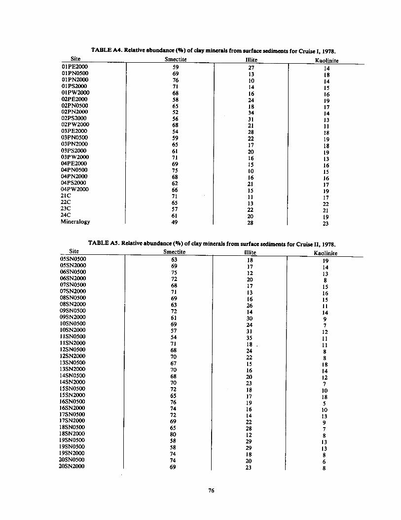
TABLE A4. Relative abundance (%) of clay minerals from surface sediments for Cruise I, 1978 . Site Smectite Illite Kaolinite

0 1PE2000 59 27 14 O1 PNOS00 69 13 18 0 1 PN2000 76 10 14 O1PS2000 71 14 15 Ol PW2000 68 16 16 02PE2000 58 24 19 02PN0500 65 18 17 02PN2000 52 34 14 02PS2000 56 31 13 02PW2000 68 21 11 03PE2000 54 28 18 03PN0500 59 22 19 03PN2000 65 17 1 8 03PS2000 61 20 19 03P W2000 71 16 13 04PE2000 69 15 16 04PN0500 75 10 15 04PN2000 68 16 16 04PS2000 62 21 17

66 15 19 21C 71 11 17 22C 65 13 22 23C 57 22 21 24C 61 20 19 Mineralogy 49 28 23

TABLE AS. R elative abundance (%) of clay minerals from surface sediments for Cruise II, 1978. Site Smectite I(lite Kaolinite

05SNO500 63 18 19 05SN2000 69 17 14 06SN0500 75 12 13 06SN2000 72 20 8 07SN0500 68 17 I S 07SN2000 71 13 16 08SN0500 69 16 15 08SN2000 63 26 I 1 09SN0500 72 14 14 09SN2000 61 30 9 l OSN0500 69 24 7 lOSN2000 57 31 12 11 SN0500 54 35 11 11 SN2000 71 18 . 11 12SN0500 68 24 12SN2000 70 22 8 13SN0500 67 15 18 13SN2000 70 16 14 14SN0500 68 20 12 14SN2000 70 23 7 15SN0500 72 18 10 1 SSN2000 65 17 1 8 16SN0500 76 19 5 16SN2000 74 16 10 17SN0500 72 14 13 17SN2000 69 22 9 18SN0500 65 28 7 18SN2000 80 12 8 19SN0500 58 29 13 19SN0500 58 29 13 19SN2000 74 18 8 20SN0500 74 20 6 20SN2000 69 23 8

76

TABLE A6. Relative abundance (%) of minerals in bulk samples for Cruise I, 1978 .

Calculated from Total Clay

y V

c, T

~ ~

- a y

d O .".

Site p~ a ~-4 U A ~ F~~ ~n a ~E ~

O1PE2000 61 16 8 1 3 2 9 5.3 2.4 1 .3 2.2 0.5 4 .2 1 .9 O1PN0500 61 11 10 6 1 3 8 5.5 1 .0 1 .5 5 .3 1 .4 3.8 0.7 OIPN2000 63 6 7 2 3 5 14 10.6 1 .4 2.0 7.6 1 .4 5.4 0.7 O1 PS2000 58 7 8 3 3 4 16 11 .4 2.2 2.4 5 .1 1 .1 4.7 0.9 OlPW2000 57 20 5 3 2 4 9 6.2 1 .4 1 .4 43 1 .0 43 1 .0 02PE2000 65 11 8 2 4 2 8 4.6 1 .9 1 .5 2.4 0.8 3.1 1 .3 02PN0500 64 7 7 2 4 3 12 7.8 2.2 2.0 3.6 0.9 3.8 1 .1 02PN2000 62 19 5 1 3 2 9 4.7 3 .1 1 .3 1 .5 0.4 3 .7 2.4 02PS2000 64 22 4 2 1 2 5 2.8 1 .6 0.7 1 .8 0.4 4 .3 2.4 02PW2000 64 8 12 2 3 4 8 5.4 1 .7 0.9 3 .2 0 .5 6.2 1 .9 03PE2000 54 21 10 1 3 3 7 3.8 2.0 1 .2 1 .9 0.6 3.0 1 .6 03PN0500 59 27 3 1 1 3 6 3.5 1.3 1 .2 2.7 0.9 3.1 1 .2 03PN2000 78 3 2 3 3 11 7.2 1 .9 1 .9 3.8 1 .1 3.6 0.9 03PS2000 80 4 2 2 3 3 7 4.3 1 .4 1 .3 3 .1 1 .0 3.2 1 .1 03PW2000 68 10 8 1 1 7 6 4.3 1 .0 0.7 4.4 0.8 5.5 1 .2 04PE2000 65 4 11 3 2 5 10 6.9 1.5 1 .6 4.6 1 .1 4.3 0.9 04PN0500 60 9 7 3 3 4 14 10.5 1 .4 2 .1 7.5 1 .5 5.0 0.7 04PN2000 68 10 4 3 2 4 9 6.1 1 .4 1 .5 4.3 1 .0 4.3 1 .0 04PS2000 60 12 6 4 3 5 10 6.2 2.1 1 .7 3.0 0.8 3.7 1 .2 04PW2000 54 7 14 3 6 4 11 7.3 1.7 2.1 4.4 1 .3 3 .5 0.8 21C 52 36 3 2 2 5 3.6 0.6 0.8 6.5 1 .6 4.2 0.7 22C 62 9 10 2 3 3 11 7.2 1 .4 2 .4 5.0 1 .7 3.0 0.6 23C 62 9 7 3 4 4 11 6.3 2.4 2.3 2.6 1 .0 2.7 1 .1 24C 68 6 9 2 2 5 8 4.9 1.6 1 .5 3 .1 1 .0 3.2 1 .1 Mineralogy 64 11 11 1 3 5 5 2.5 1 .4 1 .2 1 .8 0.8 2 .1 1 .2

77

TABLE A7. Relative abundance W of minerals in bulk samples and clays for Cruise II, 1978 .

Calculated from Total Clay

Or ^

a ~ v V

$ v ~ � V e .~

~

w z o

° n Site a U ~E A ~ [ ~ .. 0SSNOS00 S1 S 10 14 S 2 13 8.2 23 2.5 3 .5 1 .1 3 .3 1 .0 0SSN2000 64 8 6 2 6 2 11 7.6 1 .9 1 .5 4.1 0.8 4.9 1 .2 06SN0500 40 10 13 2 12 23 17.3 2 .8 3.0 6.3 1 .1 5 .8 0 .9 06SN2000 49 9 11 4 1 11 16 11 .5 3.2 1 .3 3.6 0.4 9 .0 2 .5 07SN0500 S1 6 6 S 1 6 25 17.0 4.3 3.7 4.0 0.9 4.5 1 .1 07SN2000 40 3 3 4 9 41 29 .1 5 .3 6.6 S.5 1 .2 4 .4 0 .8 08SN0500 56 10 9 2 2 3 18 12.4 2.9 2.7 43 0.9 4.6 1 .1 08SN2000 51 20 4 3 3 3 16 10 .1 4 .2 1 .8 2.4 0 .4 5 .7 2 .4 09SN0500 45 6 11 2 4 32 23 .0 4.5 4 .5 S .1 1 .0 5 .1 1 .0 09SN2000 43 7 8 5 1 11 25 15 .3 7.5 2.2 2.0 0.3 6 .8 3.3 IOSN0500 73 6 7 1 2 2 9 6.2 2 .2 0.6 2.9 0.3 9 .9 3 .4 lOSN2000 79 3 3 1 1 3 11 6.3 3 .4 1 .3 1 .8 0.9 4.8 1 .1 11SN0500 75 4 3 3 1 4 11 5 .9 3 .9 1 .2 1 .5 0 .3 4 .9 3 .2 11SN2000 65 5 3 3 6 18 12 .8 3.2 2.0 3.9 0.6 6 .5 1 .6 12SN0500 60 12 4 3 3 4 16 10.9 3 .8 1 .3 2.8 0.3 8 .5 3 .0 12SN2000 54 10 5 2 2 S 22 15 .4 4 .8 1 .8 3.2 0.4 8 .8 2 .8 13SN0500 48 8 8 4 9 23 15 .4 3 .5 4 .1 4 .5 1 .2 3.7 0.8 13SN2000 37 6 S 6 3 15 28 19.6 4 .5 3.9 4.4 0.9 5 .0 1 .1 14SN0500 46 16 S 4 5 S 18 12 .2 3.6 2.2 3.4 0.6 5.7 1 .7 14SN2000 49 9 7 4 10 5 17 11 .9 3 .9 1 .2 3.0 0.3 10.0 3 .3 15SN0500 51 S S 10 2 6 22 15 .8 4.0 2.2 4.0 0.6 7 .2 1 .8 15SN2000 S 1 9 3 11 1 7 18 11 .7 3 .1 3 .2 3 .8 1 .1 3 .6 0.9 16SN0500 59 8 S 2 2 7 17 12.9 3 .2 0.9 4.0 0.3 15 .2 3 .8 16SN2000 75 4 2 1 2 1 15 11 .1 2.4 1 .5 4.6 0.6 7.4 1 .6 17SN0500 38 10 10 11 3 6 22 15 .9 3 .1 2.9 5 .1 0.9 5 .5 1 .1 17SN2000 39 8 8 15 4 10 16 11 .0 3 .5 1 .4 3 .1 0.4 7.7 2.4 18SN0500 49 13 11 3 7 6 18 11 .7 5 .0 1 .3 2 .3 0 .3 9 .3 4.0 18SN2000 52 16 6 3 1 4 17 13.6 2.0 1 .4 6 .7 0.7 10.0 1 .5 19SN0500 72 6 11 1 1 1 8 4.6 2.3 1 .0 2.0 0.5 4 .5 2.2 19SN2000 69 9 6 1 1 1 13 9 .6 2.3 1 .1 4 .1 0.4 9 .3 2 .3 20SN0500 55 11 11 S S 4 15 11 .1 3 .0 0.9 3 .7 0 .3 12 .3 3 .3 20SN2000 59 7 S 4 5 5 16 11 .0 3.7 1 .3 3 .0 0.4 8.6 2.9

78

APPENDIX B

EXPLANATION OF CONTOURING

79

APPENDIX B. Explanation of Contouring

Basic contouring rules and common sense were used in contouring the maps in this report. Contour lines are lines that connect points of equal value, or rather, lines connecting points of equal value above or

below some reference value such as a datum plane . In this case, they are lines of equal percentage points, not less than zero nor greater than one hundred . Their position on the map is decided upon rather simply, in the following manner . Where there are areas of no control points (data points), the distance between contour lines is determined at the last ones . For example :

30

* 35 038 40

If two groups of control points indicate two different spacings, the change in spacing should be gradual, not sudden . Correct :

X19 20

025

018

30 ~ 28 034 032

Incorrect:

918 X 19

20 025

032 30 929

032

If there are two points on a map of 20% and 40% sand, it can be assumed, correctly, that a point with the value of 30% sand exists somewhere between the first two points .

20 ~, 30 40

I I

Because no other control points are found between these points, the position of the 30% contour can be assumed to fall in the middle . There are, however, two exceptions to this rule .

The first occurs if there is a third control point. For example:

81

35 20

30 40 I I

In this instance the 30% contour line cannot be placed in the middle, obviously, and must fall closer to the 20% contour than the 40% contour .

The second occurs when there is an obvious slope that is steadily increasing or decreasing in its angle. In this case the placement of the contour is dependent on where the other contours are placed . For example:

1

f 10 20 30 O4p 50

I I t

In this case the 40% contour line should not be placed in the middle, between the 30% contour line and the 50% contour line, but should be closer to the 30% contour line . A change in direction of a contour line indicated by the control points should be matched by the neighboring con-

tour lines if no other control points influence them . Correct:

"]

,~ 10

Incorrect :

X16 024

20

26

In contouring the regional maps, data from Platforms 5 through 20 for Cruise I, May 1978, and Cruise III, January 1979, was not available . Such a large percentage of control points could not be ignored, so values for these platforms were taken from Cruise II, August 1978 . The justification for this was that if no values were used, the maps would be drastically changed; however, the values used would be roughly in the neighborhood of the correct values and would shift the contours only slightly .

Using these rules as a guide, all the maps in this report were contoured.

82

07 t1 1O

APPENDIX C

MAPS OF REGIONAL TREND

83

APPENDIX C. Maps of Regional Trend

Regional trends in sediment texture over the entire study area are shown in the following maps. Maps are dated according to Cruises I, II, and III as 5-78, 8-78, and 1-79, respectively .

Distribution of sediment appears to follow expected trends with one major exception . As expected, sediments near shore have a high percentage of sand . The relatively high energy environment near shore would allow only the larger, heavier particles to be deposited . Farther from shore, in a lower energy environment, fine sediments would be depos-ited . This is what was found . The exception occurs in the fact that the very fine particles, clay, are found in higher percentages farther inshore . There are some possible explanations for this: 1 . The clays are flocculating and being deposited as larger particles near shore. 2 . The clays are being brought back towards the shore during periods of quiet water by subsurface currents strong

enough to keep the clays suspended but not the silt size particles . 3 . The clays are adhering to the sand particles . These clays are then separated from the sand during the laboratory

analysis .

85

00 a

. .pat c :eJ,r IS,,' . ; , . . ~ IJUIIpFN COY 4

MOUMA L e

hd M% + ~ `oo

GOLDEN r -MEADOW 1~ 0,

> `\J`\

° tilt/ ~ ~ vEn~ltd\!~\

GkAND I sLc

Ieneocr-1. BOY fl ` ' .O%

30 /o ~l0

~.- -

7

bU

50% 4U 9 . .- a . . O ~ . . .

10 14 " 2D

PERCENT SAND (5-78) " STUDY SATES

S-'aj E p '0 iG 40

r.r., .rtn - -- .

00 v

J `- -

MGFG0.N CITY JJ ."

` X19 to O

I

" O i. . .~

n 50% -

70% ---60% - --- - ---

PERCENT SILT (5-78)

VIN'(! 'A,

' N

II ~'

_5l( r' -

STUDY SITES

SCALE o z:) h

r ~~^na~

00

MOVMA

CO�~~4 \ Y~ ~ Bo

X3.5 iiD

\~. / "

6 :3

7 . 0*--~

GRAPHIC MEAN (M Z) (5-78)

V(NIC L

I)" ~6 )/ ,J

9

I . .

O STUDY SITES

2 !0 40 ...~a-~_ ..~...

y "` MONvA'1 CI11'

~ll

J

I f

O

.14

9

'off' o ~` -C. ~ vvCttr'~

*21 GRAND 21 ISLE

... .. . .. . . . . . . . . . Teeoame say .. i

U yor ,

` /. .2 2o

i~ . . : Z <^

. t',.. . 7 .... ;f

.q . . .

23

INCLUSIVE GRAPHIC STANDARD DEVIATION 0 STUDY SITES

(Q I) (5-78) SC ti.E c ~o r,o

,~ Y)° DO a (( ~MCRG4N CITY

` MOUM4 4 i

t, _J~ v` \~

o.~ y"I

`% J fq 1

g' GOLDEN MEADOW

C\ J~ ~ _ lo ~h Au Fey L a

yU ~,Uor

' J ~ i a /iNOR:AN CITY 30 9~'~ `\ w

MOUMA

` \1 1

\\ i

/~ `moo '~ GOLDEN MEADOW

A. I ` ~. vl r: :Ct ~.~

,, G ~5 .~ \ tevre -o ew~ne Be,

12 . .

a

1 .5~ .0~

GRAPHIC KURTOSIS (Kg) (5-78)

" STUDY 517E5

SCeU E 'o 21: V) 40

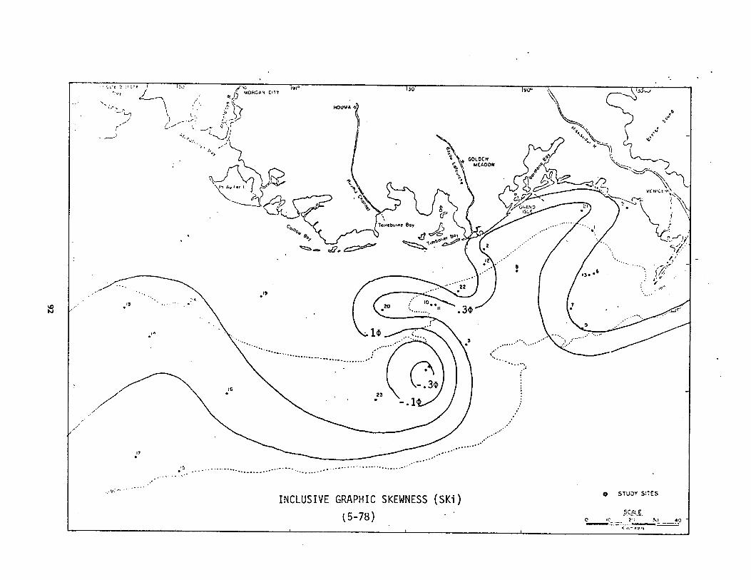
N

MO(t'v011 CITE

1\ MDUMA

`~J'

`~GOLOCN o MCADOW

1` ~. 22 . . ..1,

.

I

V~.~I:GY~r `, (° I5~

2 ,.,.

2 j :

q

i

INCLUSIVE GRAPHIC SKEWNESS (SKi) (5-78)

o STUDY S;Tcs

� ry E - k ~ 4 0

TelieDur-e Boy Cp~~oy

i6 _ . . - . . . ._ . .

MONyAN GTR )v / 4

o MOUMA4

1

m 1~ ~ k I

¢o~ ~ `�,----GOLDE N MEADOW dN~

o v~ ~ \l \ f ~ /^

vlN1Cl

w

GRL ~p \ z . 'o~' ~ ~y ` ~r J} \

TareDcmn~ Boy io J J ~' 4e

--

70°/ 60% " 6 ~~^ -

\, r_`~ .

80 . t° . 40 Zo , ; 50% . . . . . .

.: ~

. . .

20% __ 30%

10% . .

. .

PERCEfJT SAND (8-78) 0 STUDY SITES

SCALE 0 ~0 2u ]p 40

i ic�am

. . .,~ Lov bion :ne 3~ y~o 130, l9a,

<,

" ~: n~, '+ro Cl t i

~ GOLDEN & MEADOW

A

Co Terreoo~ne

d m c~. G~

+D ` E

~~ 2 q 20% " .. .

30% 4u% ~ Oq \ ~ . . .

Uqv . . . . . . . 50% ~ . . . . . . . . . . . . . - 0

70% . .

p/ 23

" 80/o

PERCENT SILT (8-78) " STUDY SATES

SCALE U iU tl 30 i ~o .e~a~

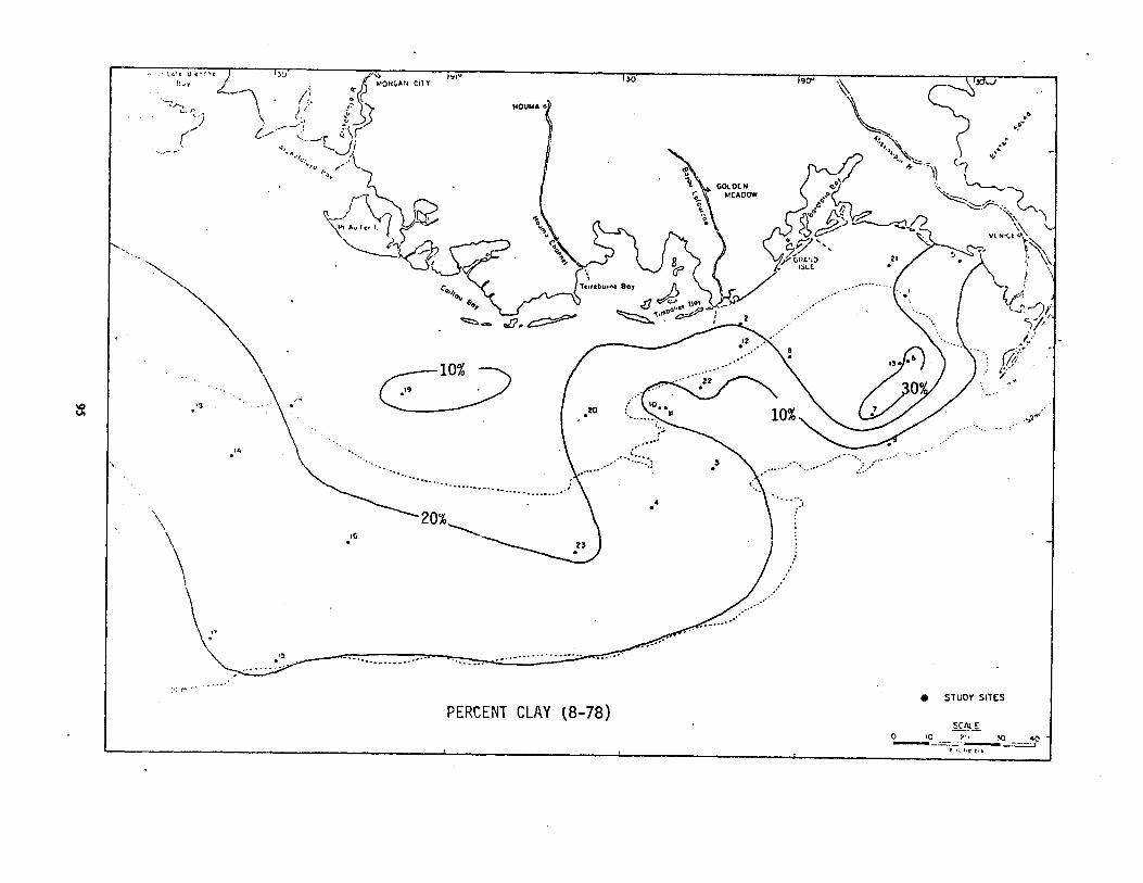
:off B'0-e

L :T

^. r i * ;,, .;;

Nol

VC v~Cl r

~GutnD 2~ iAE

1 say . . . .... .. . . . . .

Col ' ` ;

J 12

..

20 10-11 Oh '

PERCENT CLAY (8-78) " STUDY SITES

scan: o 10 -~ ,o ae

, . - -

l :l i~? ,/ 1U . /[ MOH4pN COY

l'. NOUMA 4

GOLDEN rtCADOw

o

r~ r

T 1U A!'JR(,AN X171'

e HOUMA

n

. .

b~ \,

., o.,

colocN ^`~ ~ so o` MCADOW o^

S h ~J\\ \~.i~�~

v;N~Ct

4 e ~o~ Y/ !\..

H ~GHL!:! ~ C

'v , P /y ~s.c \ 7uleea-. BOY ,R

Cfi . , `' 2

it ~~ .

3 .5 U .

1: ~9 70

20 lo . . 7

- .5c .9

i, . .

i . "

. . .. . . 60

. . .

" :n

GRAPHIC MEAN (Mz) e STUDY SITES (8-78)

" Cm F

- -- -

J

_L'~ :1 .'.n :l~t

. . =; iJ ,\ 4

2 ~MORGAt1 CITY 30 901 \

MOVMA J

_~ "\J,(

GOLDEN 0°~~ MEADOW e

~ o do ~

J ~ C~2d \H Pu Fer 1. s° '~ ~(

~' S7

. . . . . .

---------------------------

--------- I

.7

k

`4,

V`'

` ~

~lx~ted`

8 GRAND ` ~ . s P ISLE

C Tenew+nne say ~ oiip~ ~ I l ,. ~ /~7 Bo rio

4m ~ ~,1ImoW

., "01

35 ' .2Z " . ~ .5~ .~~ ' .. . . e..

20 . .. .9 . . . . . .

,. . / 1 ID

" . .. S

z3

" L'4~

INCLUSIVE. APHIC STANDARD DEVIATION STUDY SITES

(ai) (8-78) Lcn~ E

0 0 M . --AD R.If . t1

NO 00

/" �"MpHGAN CITY o (, IJ

_. . 1

~ t . \\ MOUMA i

1\~ i q~ -~J(i

/` .

" g GOLDEN ;~ MEADOW

p\L.../ L ~ v \st ao ~e~ i . ,~` ~ ~

F-=,~

i

.9,p ' CoI/'o V O

U

TensDOnM Boy

v~ ber �.,

~,, i i

9

v G. Gt:D ` ~ ~1 ISLE

.67tv." .~

'X31

oe

0

V(NI~! V

1 .11 d ' zz . .

. . ~0

. ~ . . . . . .y1 ;. .

1 .5 .9 . . .

. . . . . .. . . . . . . . . . . . . . . . . .. : . . .

w " zs

GRAPHIC KURTOSIS (Kg) 0 STUDY SITES

(8-78) <

e o b <c <<

S

+ .+ ! or .. NOqGet4 CITY /~ v- ~

tra r 1 I , ' NOUMA

1 .J~1 ' / / (

C.

1^ ~O

A,. yI ``

A~~1\

GOLDEN jj r _ o hp, EaDOW

J a~ o

8 `~Gfe4:iD 21 IS :(

Taneeo.M, 80y "'

Y nor e,

- :z

. . 22

20

9

. . . . . 1 . . . . 3o

23

I

. . INCLUSIVE GRAPHIC SKEWNESS (SKl ) 0 STUDY SITES

(8-78) p ,~ 2. . k,

-:--

C" VLNIC :<'`\ \\

I

1

. . . . . . . . . . . . . . . . : . . . . .bln.

(r ., toy / , y M(1Ru0.71 CIIY ~~ 90"

MOVMA 6 \' _

i , ~/ 1 r C

'mar MEADOW oPC \\

"GOLDEN ~~ /\,~\J C l~

cfla l,

. .

8

5% l o TerreUa~n~ Boy

o L` T U

lU%

15% 22

10 o , 15 '

. . . .-n .. . 20%

: : . . ., ~

..

. . . . . . . ~ t .

4 C5

2!

---lU7b

.. . . . . .. . . ..

r.

SMECTITE (8-78) O STUDY SITES

S~~ .E 40

r. c+aers

Pci J NCkGAN CITY ~~ 9~' `\ ~\

MOVNA 4

\\ __ _ e

` w {'~ /' ye

V v ~ 1 / ^

GOLOSN NCAGOW P(

~{,~ J So \ ,.

\\\Vt Au Fir I . 4

JlR, \ \ v 'till/ n, vU.i,l "r

0

0 Gil

Tenebuim0 Bay

`\ !.

70 ~S . " 1J'

.`\`~. 8(0-

.~~ . . `'

5U% " '

10% 4

20

2!

..

.S . ._ . .. ._ _ . . . . . . . ...~ ... . .

PERCENT SAND (1-79) O STUDY SITE;

SCn : F e ~~ 40

N

tisC~

~~0 9L \ _.-_ \]Ue.J

NOUM114 \ `r\,J

Il,

t. (`. _ 7 / ~ 4~1~

GOLDEN MEADOW

0

l ~Lo Avfu ~ .

~ G~( ~tY

P 7areDO~rt Boy n Co~~~o

CII LJ ~ ~

~1~t~ so,

ci V

to , " .

19

_,,20 . .20 . O 11

30% 407. : .: .

30~ 51 ~1l . ., . . . . . . . . . oL _ ~ 60%

. . . 40

.~ 70% z3

.,.\

., . . . . . . . . _ . . . . . . .

PERCENT SILT(1-79)

'~l_C/ C, i\ VCwKtOT\

rar:~ SLC {

i

v°

44 . . .

e STUDY SATES

2Q -14-L 0 ~o z; . 30 40

3u ,~' "v /(- MON',6N CITY

o i

4( r C )

i

' o~

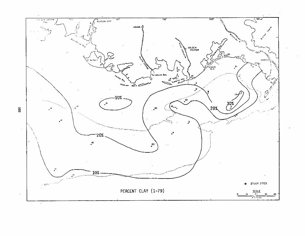
w

uCnGnn COY

MOUMA

~, GOLDEN

. A

MEADOW

%

Te"aw.- boy

2

. . . ... . . . . . . . . . . . . . . . . . . . . . . . . . . . . . . 0%-

10% ~ . . . . . . . . . . . . . . . . . . . .

PERCENT CLAY (1-79)

;-'

y

0 STUDY SITES

5cnI . e ~o z" ~o .o

-- T~c-

° . . . . 10

L .

4

i~e r

`o ~s

!J- ,Uc

`\` ~ \

S ~ ~ VIN C! \'

C \ ~Y-

~~-`Gi1LIJD 211 iS.E

. . . ~. ~� y'I f~~;

.. ~L. S~

Y~ :,

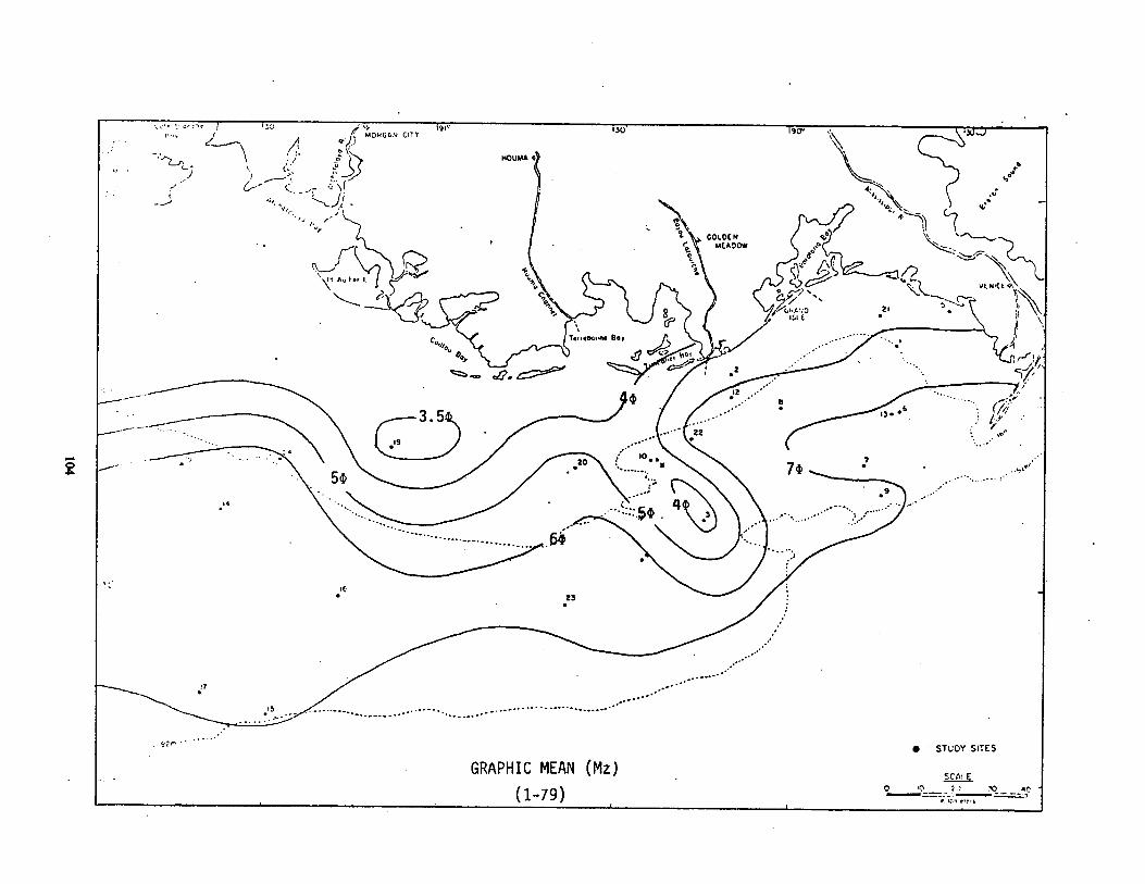
A

191, r3-u OkcaU COY . . I~'M lv^ ~. Q~1 o ~r

MOVMA S

r` L'

GOLDEN o ~ MEADOW r s , .

--,rr

Vf NBC!

:SL.E i

l Tenteonn. say /~ . . . /'

y BOy CJ ,e~ h~7 . ~ ~SYI

Zo. G~ ' .z -- ~

� , . ---.~ 3 .5 2E

i9 ~ ..

20 lo . .

54, '~ . . . .14

. . . ".i

-` it " 23

.'

, . . . . .

GRAPHIC MEAN (Mz) (1-79)

" STUDY SITES

SCn! E e ~o a :~ e --- ---- ~e ~: r n

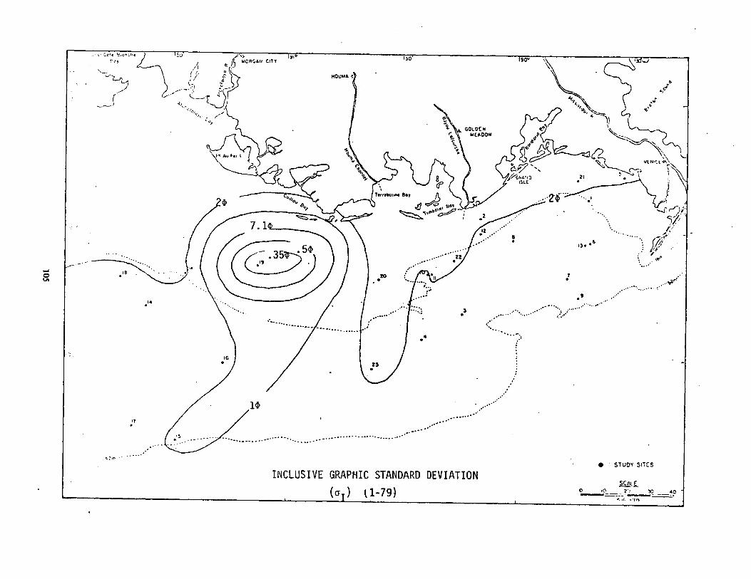
U

°~ Y ,~CR(IGN CITY -` 130 190,

~.~ //. . (\\\) MOUMA

o l

L ._ v

c,` io. --

d g

GOLDEN ~,e4~ MEADOW

c ~,B° �~ ~J~

` `\ VCN _tA`\

C,y~ ~ ~'~`.~; r\ O l

~~G6L'i~ ` : ~ ~ ` ISLE

r-! o

°°

Tvmeam0 Boy ,. .?1Y.. . . . . ~ JJ G Y' ' ,' - ;

B~ ~f l/c:V Hog `.r'ry , 7 .1 :2

b .6 . 35 . 5~

v . III . , .-y1t, ., .

7 020

.. . . ~9

.14 .. . . . . . i .. . . . .. .

.. . . ....... .... .t~

z' - _

IT

0 STUDY SITES

INCLUSIVE GRAPHIC STANDARD DEVIATION scti&-

e .o z ~ l 1x ,o -79 ) --__---~ --.~.

H

~o A y,o

~ ~, ` \ <u~

MO-GA14 CITY

-~\\ o (((\\\ MOVM4

~ t (,

.. ~~ V L__ ~ c 1

, ~

Cp"Q

f . .

r

.9(1

(4

.1

GOLDEN

I

MEADOW ~.r P

Ter~eDUru~e Bay

A G'%v

_ ticJ ~ .TOON,1

e

i

v \

~ y~ - V~~ '1\

. .

/.:

u 6 .9,p

1 .11 " -yt

1 . 5 ..~~ .. . .-~, . . . . . . . :~~

~>

GRAPHIC KURTOSIS (Kg) ~ STUDY SITES

(t-79) S«y.E o ~o z ;~ so , o

r. c-ren

/C M.CI's4N COY

NOUMA

Y GOLDEN ~ MEADOW 0

0

1 :

J,O

`a e

w V [\ ~ Z`Y

"mil. 7

V ~~J' G y^? ~.

:» ` '. P E

,� TeneWr .e Boy

r "a, V

, .

e 1~ 6

. . . . .

. 1D .ZZ. . - ' " . .

10 . . .20 . . .. ~~ ~

. r'

.. .... . - i.

. . . . . . . . - .3,t ' .

_,

t .3~ ,5 . . . . . . . . . . . . . . . . . . . . . . . . . . . . . . . . . . .

. . . . . . . . . . . . . . . .

INCLUSIVE GRAPHIC SKEWNESS(SKi) (1-79)

r `. ^\

. .

L

" ' STUDY SITES

IC A!, p " n ;" rv_ a0

APPENDIX D

COUTOUR MAPS OF INDIVIDUAL PARAMETERS AT PRIMARY PLATFORMS

109

APPENDIX D. Contour Maps of Individual Parameters at Primary Platforms.

Data on sediment texture at individual platforms is presented in the following maps, which show the four Primary Platforms and the sampling stations occupied at each . Maps are dated according to Cruises I, II, and III as 5-78, 8-78, and 1-79, respectively . Ten percent contour intervals are drawn for sand, silt and clay; one phi intervals are drawn for mean, standard deviation, skewness and kurtosis .

111

13

A 20 2s

30 -

~3/ 1b 2 ` 43 r" ~ ~1 0

Tq i 4 (j 3b 1.28 . 13

12

18 Motors

0 1000

1

A 82

N 78

"80

7s ~3 78 79

54 . ` 67 ' 73

t80 0 77

\~ ~`7 4 70

`\ \ 60 '50 v--30 Miters 28 0 1000

3

" PRIMARY STATION " SAMPLING SITE 10%CONTOUR INTERVAL

A '' -30 N

30 I-E) 40

~ 50

0A 70

5073 ~ o~~ 130

30

37' ~ =-20

14

18 Motors

0 1000 U3CK::= ]

19 A N -10

O1 0

i qi g

~ is 0 04

0 Motors 10000

4

Size SAND

Date 5-78

112

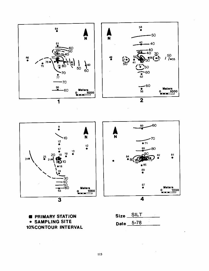
64 A N

61 -160 (~0~50 `40

66 7 " 6 `81 e ~ 6. " Il

75 so1 381 ,~ ~ 60 ~ 50 6 70 .

n 70

50 60 Motors

0 1000

1

8 ,o

12 t

17 13

Q 18 19 0 31~

1 s! 10 "18

19 .

30 -40

50 -r-60 63

A N

12

Meters ~~ 0

3

" PRIMARY STATION " SAMPLING SITE

10%CONTOUR INTERVAL

A 58

_~ 50 N

~- 40 -40 40 30 50 49 ~ 1055 0~3~36~~tl

5a 41 '411\ 50

60 62

,..-.--60 Motors

56 0 1000

2

60 60

A _~70

X71

80 80

-

0 82 81 84

73 ~ 76

0 85

89

87 Meters

0 1000

4

Size . SILT

Date 5-78

113

23

14

15

s 18 "^20 29 . 12

11

-20 22

A N

,2

Motors ~O

1

R

9

3 8

14 7 5 g 2 0

07 10

6

7

9

A N

9

Motors ~0

3

" PRIMARY STATION " SAMPLING SITE

1090 CONTOUR INTERVAL

A ,5

N 1s

20 1 22

20

1

8 6 14 4191 31 10" C ~ 10~ 40 30 "

11

22 d,

24

zs Motors

0 1000

2

A '9 -20 N

22 20

7 1i~ l 1

lor " -10

8

t 8

9

14

Motors 0 1000

4

Size CLAY

Date 5-78

114

6 .4 oP A 6 N

5~ 7

5.30

6.46 5:9 59 .j6 5 47 6.35 6.69 19

6 .03

,s 5.90

5.29 Meters

0 1000

1

2; A -'3 N 3.16

3.44 3.42

3.J0 4.g7 ` 3.j6 /3]28 03.80

3.74 X3.22

3.54 X3.82

4

5 Motors 5.40 p 1000

3

" PRIMARY STATION " SAMPLING SITE

10 CONTOUR INTERVAL

A 54J2

N 5J8

5J0

6,J8 4,~3' S~5,1 l ~74 5.45 ~ -5~ 5.49

s.sa g

6.&6 Meters 0 1000

2

A 642

N 6 . ;3

6.46

6~~3 5~fiT . 6.16 6.42 6.J4

6.a5 5.8p 6.82

6 5.~1

Meters 0 1000

4

Size _ MEAN

Date 5-78

115

2 ;8 A N

2 .24 t

2 .:0

2 2.04 .~1 2 26 3 ~

0 ,

1.19 1 ~ Z.i$ . 1 .83 2.39 .2g 2J9

`2 .t06

1 .89 `'

2 ..4 Motors

0 1000

1

,gs A N

1 .85 t 2 2~8 1 .56

1 .93 ~g

2~8 2 0 1 .30,5 ~i4 ~ ~r

1 .78 0 1.61

1 .78

1 .99

2i5 Meters 0 1000

3

" PRIMARY STATION " SAMPLING SITE CONTOUR INTERVAL

2 .;3 A N

2.16

2 ..2/

2.41 41 3 .06 ,1 t ~ ~ ~ 2 0

1 .19 - . 2 19 . ,

2 .12 2

221

t 2.34

2.40 Motors

0 1000

2

A 2.30

N 2.06 t

1 .83

1 .66 2.06 -~2 1 .48

1 .72 " it * , s~ t 0 . . 1 .78 1 .33 1.60

1 .39

1 .47 Motors

0 1000

4

Size STD . DEV .

Date 5-78

116

,6

.18 A N

o 25 ~ o ~ . l .32 .21 .p5 .17 ` .61

.16

.15

.27 Motors

0N ~1~000

1

_.,o so A N

. -.5 .58 . 68

.55 0 .65

- 6j

.3 6 .6: 3 0

0 ' : . : k .52

.5`

.55

.649 ,-.5

-i-0 Motors p 1000 mK===

3

" PRIMARY STATION " SAMPLING SITE 1 CONTOUR INTERVAL

i1 A N

.54

.43 0

4io 5 2 6214 ~ 400 .21 ~?1 .9

.32

-1

1 .43

J5 1

Meters O 1000

2

A 24

N .04 -.(i5

.4 .02 '21 .05 'i31 'i3

.07 t .21

Motors 0 0

4

Size SKEWNESS

Date -5-78

117

.94 Is A N

.91 t

.92

.96

.~2 98 .1 .2 1 .61 , .g9 I

1 .09 /

100, 1 1 ~ .

1 .90

Motors 0 1000

1

3.22 t A

N 2.84

3 7 2.55 95 2

~ .

:3 2.242618 / ~ ~ i ~

~i i .os K 2.1s o

11 ~ .7 "-2

~ M t 9 o ors .82 p 1000

3

" PRIMARY STATION " SAMPLING SITE 1ldCONTOUR INTERVAL

A 1" ' N

1 .21 t

1 .49

.97 ,p2 ~ t `

C~ 1J5 ! 1 .96 49 . 2 .75 .

1 .47

.83

'i Motors 0 1000 m=

2

A N

1 .01

0 1-16

18 21 .23 1J8

. 1 ..8 1 5 ~ f

16 1 .73 ~'

1 .47

1 .76

1'i5 Motors 0 1000

4

Size KURTOSIS

Date 5-78

118

'4 A j0'1 N

1 05 I 211

" r9 "+

I 15

20 09 t lp 2 O 30

14 Motors 0 1000 c3K3K=

1

9, -90

-80 0

qr,6* 79 0 53 69 0&

7'

o0

0

00 70 70 60

-50 -40

30 23

A N

Motors 0 1000

" PRIMARY STATION " SAMPLING SITE

10% CONTOUR INTERVAL

A ~-30

N

---20 _- "i ~ -

16

59 53 0

50 .00,

04e \~4-40~

30

~ --w- 20 Motors 19 0 1000

2

A N

10

9 Re 8

112

Motors 0 1000

4

Size _SAND

Date 8-78

119

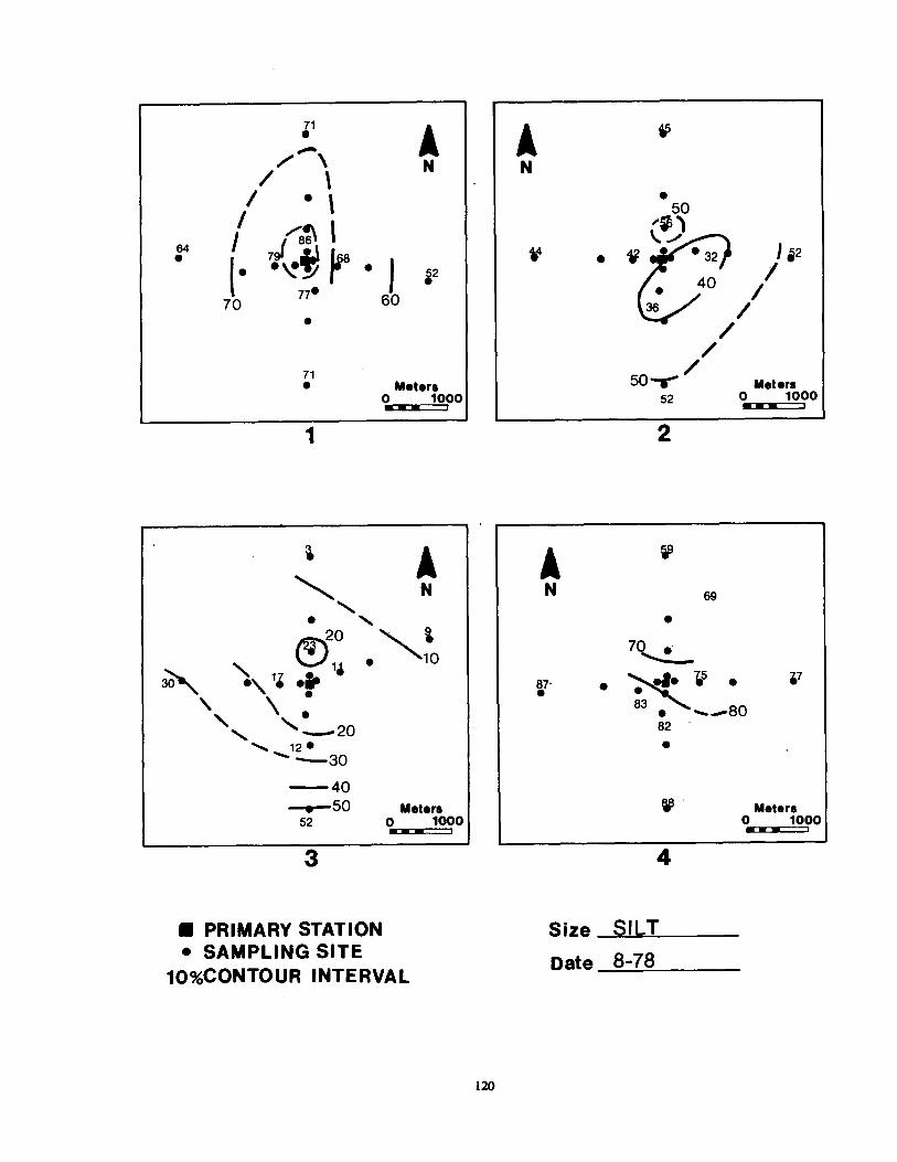
" 1 A N

/ /~8~ i sa

" t 0 ~~~ ~8 I 0 I i52

70 77* 60

71 0 Motors

0 1000

1

A N

Q20 10

.\ , j . 30

" - 20 \~ 120

30

40 --x-50 Meters

52 0 1000

3

" PRIMARY STATION " SAMPLING SITE

10,YoCONTOUR INTERVAL

A N

50

lei ~ 32 } ~ J2

r36

50-v- Motors 52 0 1000

2

A ss

70'..,-

.7. ~ . ,j. 45 . Z'

83

82

Motors 0 1000

4

Size SILT

Date 8-78

120

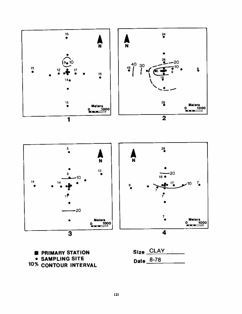
,5

A N

n (s,10

1s 12 L 17 ""j' " t 15

140

15 0 Motors

O 1000

1

5

A N

12 s -10

14 14

t

20

Motors p 1000 =3000==

I

3

" PRIMARY STATION " SAMPLING SITE CONTOUR INTERVAL

A 24

N

28 ~20 40 30 ~~ 10 R 4~ y ~ '

i

28 Motors

0 1000

G

28 A N

-20 1s

10 7 9

17

7

7

Motors 0 1000

4

Size CLAY

Date $'78

121

6.34

6.62

5.87 6.24

5.84

5.97

\6

6.10

A N

5;

Motors ~0

1

2.55 A -~- 3 N

3.49 4 3 .456 4 .69

4.07

9o 0

.6

0 0

F:O3. W8 4

0 5

6 Motors 0 6.21 p 1000

3

" PRIMARY STATION " SAMPLING SITE

1 0 CONTOUR INTERVAL

A 5+80

6

F~43 7

t~98 . ._. C -5 5.02

6 Maters

6.24 0 1000

2

A 6.74

N

6.J7

6:5 j~ spa ~ s~2

~ ' 5.92

81 5 .

6'"2 Meters 0 1000

4

Size MEAN

Date 8-78

122

1 ..9 A N

1;8 2

2i5 I 1j7 .+ ~ 1+59 1 2�es 1.73

Meters 2 .15 0 1000

1

'2 A ., 1.98

2 1 1 9 t

. .1 2 .59 2.1,20 &0 ~

t

~

2 .16 2

~ 2 .5

Meters 2.73 ~ 0

3

" PRIMARY STATION " SAMPLING SITE CONTOUR INTERVAL

A 2079

N

?r39

1 8

' (11133 1 54

2.21

Meters 2.23 0 1000

03~ 1

2

A zj?8 N

2~7 2

1.15 0 1 . 3*80 ~ ~ t.j4

1.94 t

t

I.J4 Motors 0 1000

4

Size _ STD. DEV .

Date _ 8-78

123

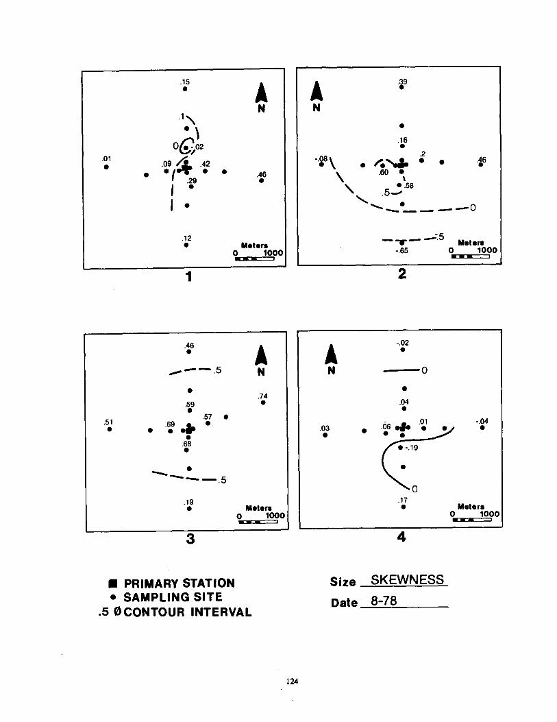
.15

A N

1

OC o2 .Ot

42 09 0 Z . .

" l" 0 0 .46 .zs

.12 0 Motors

0 1000

A 49

N

.is

- 46 .08

.so 0 .58

- .~-~0

- -W Motors -.65 0 1000

2 1

.46 t A

.000, .5 N

.74 .59

.51 .7 . .69

t .68 t

t

.is 0 Motors

0 1000

3

" PRIMARY STATION " SAMPLING SITE

.5 OCONTOUR INTERVAL

A _ .02 t

N ---- 0

.04 t

.03 .01 - .04

~ .06 ~~~ 0 0

0 -.19

0 .17

Motors 0 1000

124

4

Size SKEWNESS

Date 8-78

.86

A N

1 .02 0 1 .03 1 : ~ .9: . .

0 .79

~ .9 9

1 .04 Meters

0 1000

A .88

N

.aa

X1 .56 . 1 :2

1 .35 . 1.5

12

.78 Meters

0 1000 m===

1 2

3;4 A 3 N

2 .97 .. 1 .48 /

26 3 2 . 1 .0 1 .72 ~ '1

/ 3.09

2

Motors .83 p 1000

3

" PRIMARY STATION " SAMPLING SITE

.50 CONTOUR INTERVAL

.91 A N

d1.08

1.03 1 .61 ~ " j" t

.97 1 .43

1 .5

1 .72

1 .34 t

Meters 0 1000

4

Size KURTOSIS

Date 8-78

125

A N

12

i 16 " ,o~ . .+ . Z

19

10 - 20 15

is Maters

0 1000 mo

1

90

N

so 86 7.

79

73 -70

--.,-60

-5040

-30 y20 Motors

20 0 1000 Sao

3

" PRIMARY STATION SAMPLING SITE

109oCONTOUR INTERVAL

A 30

20

i s

10 t 47

50 52 40

-~-40 Meters

38 0 1000

2

A '' N

o

1

t

Meters 0 1000 K-~ i

4

Size SAND

Date 1-79

126

A N

g 60

s ' 75.1 .~ i

I (057- ~~"-59 '--~ 60

~%..-.*7o 0

Motors 72 0 1000

1

5 A N

" .1o

L7 5 " " , "ir

-20 --!-~30 ------40 --,50

Motors 56 0 1000

3

" PRIMARY STATION " SAMPLING SITE

1p%CONTOUR INTERVAL

A 44

50

5040

39 ~5 ~ i ~ 40 r 35

`~ ~ 30 1 /

/'

11,100,

i Motors 0 1000

A %9

N I

74

69 16 ;7 %6

70 ~ 67

Meters 0 1000

4

size . SILT

Date . 1-79

127

z' A N

%3i 30 -,,r 20 eir J3 11 ~' 1 J8 4

Meters 0 o 1000

l:mK:=

A N

30208 40 20

17 "8 / "4 18

/17

20~ Motors 0 1000

1 2

A N

to 08

0 +p

10 12 t

- 20 Meters

O 1000 ono

3

" PRIMARY STATION " SAMPLING SITE 109PONTOUR INTERVAL

16 A N

N 18

20 . :6 ~ 022 9 29 17

26/ /

20 Motors

0 1000

4

Size CLAY

Date 1-79

128

6' A N

6; 6.23 6.40 " ~ ~Z

6.63 t

5.37 6 / 5.98

5 .74 Motors

I 0 1000

1

2' A N

3 3.56

3.62 t

3.14 / 2.81 3 . 41 ..

3.99

-- 5

Meter 6.11 p 1000

mC~

3

" PRIMARY STATION " SAMPLING SITE

1 0 CONTOUR INTERVAL

A 5.77

s

1 659 J 7.47 7,j4 t " ~ 5.39 4.54 e

4.79

05

5.47 0 Motors 0 1000

2

6.29

A Is N

6.49 t

6 .. ~ . so* 6 ..7 . 6.90

6.61 t

6.55

6.52 Meters

0 1000

4

Size MEAN

Date 1-79

129

2.59

A N

2: 9

. 1:

1 2+12

772o

~ .00

- 1" .63

2.0Zr 2

1 .76 0 Motors

0 1000

1

,J2 A N

~2 1 .33

~ 0

2.17

1 .01 2 0 ~ . 6 2 .0 3

t 2.36 t

2 4 i Motors 0 1000 oC307=

3

t PRIMARY STATION " SAMPLING SITE

1 0 CONTOUR INTERVAL

A 2'8 N

2~a

242 2.07 " ~ 2.45 1 .60 /

l 1 .78

2.58 Meters

0 1000

2

A 2021

N

2,J4

~7 1 .64 2.13 ~ 1.82 "j" 1

2.1

2

1 .83 Motors

0 1000

4

Size STD . DEV .

Date 1-79

130

i A N

.17

/.5 /

.s1 .s2

0 .5 Motors .49 0 1000

1

42 o .25 I

.jo

~~.5

A N

Meters ~0

3

" PRIMARY STATION " SAMPLING SITE 10 CONTOUR INTERVAL

A .3; N

.38 t

.94 -.01 .46

0/

51 Motors

0 1000

2

A -._6 N --3

=0

07 0 .22 010 (0 .56 0 0 `.5

27

.12

.si

Motors 0 1000

4

Size _ SKEWNESS

Date 1-79

131

'° A N

.78

.83 63 0 ~ . 5 --- ~ . ~~ o zs o

.ss .72

.74 Meters

0 1000

1

3.98 A N

3.38 I

3 83 ~ ~ '1 \ . 2.61 , o~ 2.07

3.58

1 Meters

.90 p 1000

3

" PRIMARY STATION " SAMPLING SITE 1CONTOUR INTERVAL

A , .,3

N

.87

~ 5 .85 ~ ~ ~ 1 :0 "

i .os.

1 .39 t

/1 .5

i / Meters 1 .51 0 1000

2

A N

t

t ~ t t

t

Meters 0 1000

4

Size KURTOSIS

Date 1-79

132

VOLUME I-POLLUTANT FATE AND EFFECTS STUDIES Part 3-Organic Chemical Analyses

by

C.P. Nulton Principal Investigator Hydrocarbons in Fauna

D.E.Johnson Principal Investigator Hydrocarbons in Fauna

C .F. Bohnstedt Principal Investigator Sediment Total Organic Carbon Hydrocarbons in Water and Sediments

S.J. Martin Principal Investigator Sediment Total Organic Carbon Hydrocarbons in Water and Sediments

Southwest Research Institute GeoChem Research Inc. Department of Environmental Sciences 16920 Park Row Division of Chemistry and Houston, Texas 77984 Chemical Engineering

P.O . Drawer 28510 San Antonio, Texas 78284

Editor : C.A . Bedinger, Jr . Editorial Assistant: Laura Z. Kirby

TABLE OF CONTENTS

Page

I.

II .

III.

INTRODUCTION ... . . . . . . . . . . . . . . . . . . . . . . . . . . . . . . . . . . . . . . . . . . . . . . . . . . . . . . . . . . . . . . . . . . . . . . . . . . . . . . . . . . . . . . . . . . . . . . . . . . . . . . . . . . . . 133 A. Petroleum Hydrocarbons in the Marine Environment ... . . . . . . . . . . . . . . . . . . . . . . . . . . . . . . . . . . . . . . . . . . . . . . . . . . . . . . . . 133

l . Sources of Hydrocsrbons. . . . . . . . . . . . . . . . . . . . . . . . . . . . . . . . . . . . . . . . . . . . . . . . . . . . . . . . . . . . . . . . . . . . . . . . . . . . . . . . . . . . . . . 133 2. Indicators of Hydrocarbon Type. . . . . . . . . . . . . . . . . . . . . . . . . . . . . . . . . . . . . . . . . . . . . . . . . . . . . . . . . . . . . . . . . . . . . . . . . . . . . . 133

B . Other Studies in the Gulf of Mexico . . . . . . . . . . . . . . . . . . . . . . . . . . . . . . . . . . . . . . . . . . . . . . . . . . . . . . . . . . . . . . . . . . . . . . . . . . . . . . . . . . 133 C . The Central Gulf Platform Study . . . . . . . . . . . . . . . . . . . . . . . . . . . . . . . . . . . . . . . . . . . . . . . . . . . . . . . . . . . . . . . . . . . . . . . . . . . . . . . . . . . . . 133

i. Study Area and Sampling Scheme . . . . . . . . . . . . . . . . . . . . . . . . . . . . . . . . . . . . . . . . . . . . . . . . . . . . . . . . . . . . . . . . . . . . . . . . . . . . 133 2. General Design of the Present Study ... . . . . . . . . . . . . . . . . . . . . . . . . . . . . . . . . . . . . . . . . . . . . . . . . . . . . . . . . . . . . . . . . . . . . . . 135 3. Organic Chemistry Studies of Water and Sediments. . . . . . . . . . . . . . . . . . . . . . . . . . . . . . . . . . . . . . . . . . . . . . . . . . . . . . 135

a. Sediment TOC . . . . . . . . . . . . . . . . . . . . . . . . . . . . . . . . . . . . . . . . . . . . . . . . . . . . . . . . . . . . . . . . . . . . . . . . . . . . . . . . . . . . . . . . . . . . 135 b. LMW-HCin Seswater. . . . . . . . . . . . . . . . . . . . . . . . . . . . . . . . . . . . . . . . . . . . . . . . . . . . . . . . . . . . . . . . . . . . . . . . . . . . . . . . . . . 135 c. HMW-HCin Sediments. . . . . . . . . . . . . . . . . . . . . . . . . . . . . . . . . . . . . . . . . . . . . . . . . . . . . . . . . . . . . . . . . . . . . . . . . . . . . . . . . 135

4 . Hydrocarbons in Fauna . . . . . . . . . . . . . . . . . . . . . . . . . . . . . . . . . . . . . . . . . . . . . . . . . . . . . . . . . . . . . . . . . . . . . . . . . . . . . . . . . . . . . . . . . 136 a . Background . . . . . . . . . . . . . . . . . . . . . . . . . . . . . . . . . . . . . . . . . . . . . . . . . . . . . . . . . . . . . . . . . . . . . . . . . . . . . . . . . . . . . . . . . . . . . . . . 136 b . Previous HMW-HC Analyses of Fauna from the Gulf of Mexico . . . . . . . . . . . . . . . . . . . . . . . . . . . . . 136 c . HMW-HC Analyses of Fauna in the Present Study. . . . . . . . . . . . . . . . . . . . . . . . . . . . . . . . . . . . . . . . . . . . . . . 136

METHODS AND MATERIALS . . . . . . . . . . . . . . . . . . . . . . . . . . . . . . . . . . . . . . . . . . . . . . . . . . . . . . . . . . . . . . . . . . . . . . . . . . . . . . . . . . . . . . . . . . . . . 137 A. Sediment TOC .. . . . . . . . . . . . . . . . . . . . . . . . . . . . . . . . . . . . . . . . . . . . . . . . . . . . . . . . . . . . . . . . . . . . . . . . . . . . . . . . . . . . . . . . . . . . . . . . . . . . . . . . . . . 137

1. Sampling Methods . . . . . . . . . . . . . . . . . . . . . . . . . . . . . . . . . . . . . . . . . . . . . . . . . . . . . . . . . . . . . . . . . . . . . . . . . . . . . . . . . . . . . . . . . . . . . . . 137 2. LaboratoryAnalyses . . . . . . . . . . . . . . . . . . . . . . . . . . . . . . . . . . . . . . . . . . . . . . . . . . . . . . . . . . . . . . . . . . . . . . . . . . . . . . . . . . . . . . . . . . . . . 137

B. LMW-HC in Seawater . . . . . . . . . . . . . . . . . . . . . . . . . . . . . . . . . . . . . . . . . . . . . . . . . . . . . . . . . . . . . . . . . . . . . . . . . . . . . . . . . . . . . . . . . . . . . . . . . . . 137 1 . Sampling Methods . . . . . . . . . . . . . . . . . . . . . . . . . . . . . . . . . . . . . . . . . . . . . . . . . . . . . . . . . . . . . . . . . . . . . . . . . . . . . . . . . . . . . . . . . . . . . . . 137 2. Laboratory Ana/yses . . . . . . . . . . . . . . . . . . . . . . . . . . . . . . . . . . . . . . . . . . . . . . . . . . . . . . . . . . . . . . . . . . . . . . . . . . . . . . . . . . . . . . . . . . . . . 138

C. HMW-HC in Sediments . . . . . . . . . . . . . . . . . . . . . . . . . . . . . . . . . . . . . . . . . . . . . . . . . . . . . . . . . . . . . . . . . . . . . . . . . . . . . . . . . . . . . . . . . . . . . . . . . 138 1. Sampling Methods . . . . . . . . . . . . . . . . . . . . . . . . . . . . . . . . . . . . . . . . . . . . . . . . . . . . . . . . . . . . . . . . . . . . . . . . . . . . . . . . . . . . . . . . . . . . . . . 138

a. Surficial Sediments. . . . . . . . . . . . . . . . . . . . . . . . . . . . . . . . . . . . . . . . . . . . . . . . . . . . . . . . . . . . . . . . . . . . . . . . . . . . . . . . . . . . . . . 138 b. Downcore Sediments ... . . . . . . . . . . . . . . . . . . . . . . . . . . . . . . . . . . . . . . . . . . . . . . . . . . . . . . . . . . . . . . . . . . . . . . . . . . . . . . . . . 139 c. Shipboard Contaminants ... . . . . . . . . . . . . . . . . . . . . . . . . . . . . . . . . . . . . . . . . . . . . . . . . . . . . . . . . . . . . . . . . . . . . . . . . . . . . 139

2. LaboratoryAnalyses . . . . . . . . . . . . . . . . . . . . . . . . . . . . . . . . . . . . . . . . . . . . . . . . . . . . . . . . . . . . . . . . . . . . . . . . . . . . . . . . . . . . . . . . . . . . . 139 a . Sample Processing and Hydrocarbon Extraction. . . . . . . . . . . . . . . . . . . . . . . . . . . . . . . . . . . . . . . . . . . . . . . . . . 141 b . CC Analysis. . . . . . . . . . . . . . . . . . . . . . . . . . . . . . . . . . . . . . . . . . . . . . . . . . . . . . . . . . . . . . . . . . . . . . . . . . . . . . . . . . . . . . . . . . . . . . . . 141 c. GCAnalysis . . . . . . . . . . . . . . . . . . . . . . . . . . . . . . . . . . . . . . . . . . . . . . . . . . . . . . . . . . . . . . . . . . . . . . . . . . . . . . . . . . . . . . . . . . . . . . . 141 d. GC/MS . . . . . . . . . . . . . . . . . . . . . . . . . . . . . . . . . . . . . . . . . . . . . . . . . . . . . . . . . . . . . . . . . . . . . . . . . . . . . . . . . . . . . . . . . . . . . . . . . . . . . 145

D. Hydrocarbons in Fauna . . . . . . . . . . . . . . . . . . . . . . . . . . . . . . . . . . . . . . . . . . . . . . . . . . . . . . . . . . . . . . . . . . . . . . . . . . . . . . . . . . . . . . . . . . . . . . . . . 145 1. Sampling and Shipboard Processing . . . . . . . . . . . . . . . . . . . . . . . . . . . . . . . . . . . . . . . . . . . . . . . . . . . . . . . . . . . . . . . . . . . . . . . . . 145 2. Laboratory Analysis . . . . . . . . . . . . . . . . . . . . . . . . . . . . . . . . . . . . . . . . . . . . . . . . . . . . . . . . . . . . . . . . . . . . . . . . . . . . . . . . . . . . . . . . . . . . . 146

a . Dissection . . . . . . . . . . . . . . . . . . . . . . . . . . . . . . . . . . . . . . . . . . . . . . . . . . . . . . . . . . . . . . . . . . . . . . . . . . . . . . . . . . . . . . . . . . . . . . . . . . 146 6 . Tissue Digestion . . . . . . . . . . . . . . . . . . . . . . . . . . . . . . . . . . . . . . . . . . . . . . . . . . . . . . . . . . . . . . . . . . . . . . . . . . . . . . . . . . . . . . . . . . 146 c. Extraction . . . . . . . . . . . . . . . . . . . . . . . . . . . . . . . . . . . . . . . . . . . . . . . . . . . . . . . . . . . . . . . . . . . . . . . . . . . . . . . . . . . . . . . . . . . . . . . . . . 146 d. Silica Gel CC . . . . . . . . . . . . . . . . . . . . . . . . . . . . . . . . . . . . . . . . . . . . . . . . . . . . . . . . . . . . . . . . . . . . . . . . . . . . . . . . . . . . . . . . . . . . . . 146 e. Capillary Column GC. . . . . . . . . . . . . . . . . . . . . . . . . . . . . . . . . . . . . . . . . . . . . . . . . . . . . . . . . . . . . . . . . . . . . . . . . . . . . . . . . . . 146 f. Spiking Experiments . . . . . . . . . . . . . . . . . . . . . . . . . . . . . . . . . . . . . . . . . . . . . . . . . . . . . . . . . . . . . . . . . . . . . . . . . . . . . . . . . . . . . 146 g . GC/MS . . . . . . . . . . . . . . . . . . . . . . . . . . . . . . . . . . . . . . . . . . . . . . . . . . . . . . . . . . . . . . . . . . . . . . . . . . . . . . . . . . . . . . . . . . . . . . . . . . . . . 147

RESULTS . . . . . . . . . . . . . . . . . . . . . . . . . . . . . . . . . . . . . . . . . . . . . . . . . . . . . . . . . . . . . . . . . ... . . . . . . . . . . . . . . . . . . . . . . . . . . . . . . . . . . . . . . . . . . . . . . . . . . . . . . 149 A. Sediment TOC .... . . . . . . . . . . . . . . . . . . . . . . . . . . . . . . . . . . . . . . . . . . . . . . . . . . . . . . . . . . . . . . . . . . . . . . . . . . . . . . . . . . . . . . . . . . . . . . . . . . . . . . . . 149 B. LMW-HC in Seawater . . . . . . . . . . . . . . . . . . . . . . . . . . . . . . . . . . . . . . . . . . . . . . . . . . . . . . . . . . . . . . . . . . . . . . . . . . . . . . . . . . . . . . . . . . . . . . . . . . . 149 C. HMW-HC in Sediments. . . . . . . . . . . . . . . . . . . . . . . . . . . . . . . . . . . . . . . . . . . . . . . . . . . . . . . . . . . . . . . . . . . . . . . . . . . . . . . . . . . . . . . . . . . . . . . . . 149

i. Surficial Sediments. . . . . . . . . . . . . . . . . . . . . . . . . . . . . . . . . . . . . . . . . . . . . . . . . . . . . . . . . . . . . . . . . . . . . . . . . . . . . . . . . . . . . . . . . . . . . . . 149 a. Total Hydrocarbons ... . . . . . . . . . . . . . . . . . . . . . . . . . . . . . . . . . . . . . . . . . . . . . . . . . . . . . . . . . . . . . . . . . . . . . . . . . . . . . . . . . . 149 b. Saturated Hydrocarbons . . . . . . . . . . . . . . . . . . . . . . . . . . . . . . . . . . . . . . . . . . . . . . . . . . . . . . . . . . . . . . . . . . . . . . . . . . . . . . . . 1'49 c. Unsaturated Hydrocarbons . . . . . . . . . . . . . . . . . . . . . . . . . . . . . . . . . . . . . . . . . . . . . . . . . . . . . . . . . . . . . . . . . . . . . . . . . . . . 151

2. Downcore Sediments ... . . . . . . . . . . . . . . . . . . . . . . . . . . . . . . . . . . . . . . . . . . . . . . . . . . . . . . . . . . . . . . . . . . . . . . . . . . . . . . . . . . . . . . . . . 1 51 a. Saturated Fraction . . . . . . . . . . . . . . . . . . . . . . . . . . . . . . . . . . . . . . . . . . . . . . . . . . . . . . . . . . . . . . . . . . . . . . . . . . . . . . . . . . . . . . . 151 b. Unsaturated Fraction . . . . . . . . . . . . . . . . . . . . . . . . . . . . . . . . . . . . . . . . . . . . . . . . . . . . . . . . . . . . . . . . . . . . . . . . . . . . . . . . . . . . 151

D. Hydrocarbons in Fauna . . . . . . . . . . . . . . . . . . . . . . . . . . . . . . . . . . . . . . . . . . . . . . . . . . . . . . . . . . . . . . . . . . . . . . . . . . . . . . . . . . . . . . . . . . . . . . . . . 151 1 . Pelagic Fish . . . . . . . . . . . . . . . . . . . . . . . . . . . . . . . . . . . . . . . . . . . . . . . . . . . . . . . . . . . . . . . . . . . . . . . . . . . . . . . . . . . . . . . . . . . . . . . . . . . . . . . . 155

a . Saturated Fraction . . . . . . . . . . . . . . . . . . . . . . . . . . . . . . . . . . . . . . . . . . . . . . . . . . . . . . . . . . . . . . . . . . . . . . . . . . . . . . . . . . . . . . . 155 2. Demersal Fish and Macrcepifauna . . . . . . . . . . . . . . . . . . . . . . . . . . . . . . . . . . . . . . . . . . . . . . . . . . . . . . . . . . . . . . . . . . . . . . . . . . . 155

a. Saturated Fraction . . . . . . . . . . . . . . . . . . . . . . . . . . . . . . . . . . . . . . . . . . . . . . . . . . . . . . . . . . . . . . . . . . . . . . . . . . . . . . . . . . . . . . . 155 b. Unsaturated Fraction . . . . . . . . . . . . . . . . . . . . . . . . . . . . . . . . . . . . . . . . . . . . . . . . . . . . . . . . . . . . . . . . . . . . . . . . . . . . . . . . . . . . 155

3. GC/MS Analyses ... . . . . . . . . . . . . . . . . . . . . . . . . . . . . . . . . . . . . . . . . . . . . . . . . . . . . . . . . . . . . . . . . . . . . . . . . . . . . . . . . . . . . . . . . . . . . . . 155

iii

TABLE OF CONTENTS (cont'd)

Page

IV . DISCUSSION . . . . . . . . . . . . . . . . . . . . . . . . . . . . . . . . . . . . . . . . . . . . . . . . . . . . . . . . . . . . . . . . . . . . . . . . . . . . . . . . . . . . . . . . . . . . . . . . . . . . . . . . . . . . . . . . . . . . . 165 A . Sediment Total Organic Carbon . . . . . . . . . . . . . . . . . . . . . . . . . . . . . . . . . . . . . . . . . . . . . . . . . . . . . . . . . . . . . . . . . . . . . . . . . . . . . . . . . . . . . . 165 B . LMW-HC in Seawater . . . . . . . . . . . . . . . . . . . . . . . . . . . . . . . . . . . . . . . . . . . . . . . . . . . . . . . . . . . . . . . . . . . . . . . . . . . . . . . . . . . . . . . . . . . . . . . . . . . 165 C. HMW-HC in Saliments . . . . . . . . . . . . . . . . . . . . . . . . . . . . . . . . . . . . . . . . . . . . . . . . . . . . . . . . . . . . . . . . . . . . . . . . . . . . . . . . . . . . . . . . . . . . . . . . . 166

i . ToldHydtocarbons . . . . . . . . . . . . . . . . . . . . . . . . . . . . . . . . . . . . . . . . . . . . . . . . . . . . . . . . . . . . . . . . . . . . . . . . . . . . . . . . . . . . . . . . . . . . . 166 2. The UCMin Sediments. . . . . . . . . . . . . . . . . . . . . . . . . . . . . . . . . . . . . . . . . . . . . . . . . . . . . . . . . . . . . . . . . . . . . . . . . . . . . . . . . . . . . . . . . . 170 3 . Saturated Hydrocarbons . . . . . . . . . . . . . . . . . . . . . . . . . . . . . . . . . . . . . . . . . . . . . . . . . . . . . . . . . . . . . . . . . . . . . . . . . . . . . . . . . . . . . . . . 170 4. Unsaturated Hydrocarbons . . . . . . . . . . . . . . . . . . . . . . . . . . . . . . . . . . . . . . . . . . . . . . . . . . . . . . . . . . . . . . . . . . . . . . . . . . . . . . . . . . . . 172

D . Hydrocarbons in Fauna . . . . . . . . . . . . . . . . . . . . . . . . . . . . . . . . . . . . . . . . . . . . . . . . . . . . . . . . . . . . . . . . . . . . . . . . . . . . . . . . . . . . . . . . . . . . . . . . . 172 E . Synthesis of Results . . . . . . . . . . . . . . . . . . . . . . . . . . . . . . . . . . . . . . . . . . . . . . . . . . . . . . . . . . . . . . . . . . . . . . . . . . . . . . . . . . . . . . . . . . . . . . . . . . . . . . 173

J . Correlation of Hydrocarbon Contamination with Platform Characteristics . . . . . . . . . . . . . . . . . . . . . . . . 173 2 . Correlation of Hydrocarbons in Downcore Sediments with Historical Development of the

Study Area . . . . . . . . . . . . . . . . . . . . . . . . . . . . . . . . . . . . . . . . . . . . . . . . . . . . . . . . . . . . . . . . . . . . . . . . . . . . . . . . . . . . . . . . . . . . . . . . . . . . . . . . . 177 3 . Impacts of Known Spills, Discharges and Other Sources of Petroleum-activity-related Conta-

minants . . . . . . . . . . . . . . . . . . . . . . . . . . . . . . . . . . . . . . . . . . . . . . . . . . . . . . . . . . . . . . . . . . . . . . . . . . . . . . . . . . . . . . . . . . . . . . . . . . . . . . . . . . . . . 177 a . Known Spills . . . . . . . . . . . . . . . . . . . . . . . . . . . . . . . . . . . . . . . . . . . . . . . . . . . . . . . . . . . . . . . . . . . . . . . . . . . . . . . . . . . . . . . . . . . . . . . 177 6. Discharges. . . . . . . . . . . . . . . . . . . . . . . . . . . . . . . . . . . . . . . . . . . . . . . . . . . . . . . . . . . . . . . . . . . . . . . . . . . . . . . . . . . . . . . . . . . . . . . . . 178 c . Other Petroleum-related Contaminant Sources. . . . . . . . . . . . . . . . . . . . . . . . . . . . . . . . . . . . . . . . . . . . . . . ., . . . 178 d. The Mississippi River as a Pollution Source . . . . . . . . . . . . . . . . . . . . . . . . . . . . . . . . . . . . . . . . . . . . . . . . . . . . . . . . 178

4. Effects of Human Consumption of Study Ares Seafood Products . . . . . . . . . . . . . . . . . . . . . . . . . . . . . . . . . . . . 178 F. An Evaluation of the Present Study and Recommendations for Further Studies.. . . . . . . . . . . . . . . . . . . . . . . . . . 179

1. Geochem Research Inc. . . . . . . . . . . . . . . . . . . . . . . . . . . . . . . . . . . . . . . . . . . . . . . . . . . . . . . . . . . . . . . . . . . . . . . . . . . . . . . . . . . . . . . . . . 179 2. Southwest Research Institute . . . . . . . . . . . . . . . . . . . . . . . . . . . . . . . . . . . . . . . . . . . . . . . . . . . . . . . . . . . . . . . . . . . . . . . . . . . . . . . . . . 180

V. CONCLUSIONS ... . . . . . . . . . . . . . . . . . . . . . . . . . . . . . . . . . . . . . . . . . . . . . . . . . . . . . . . . . . . . . . . . . . . . . . . . . . . . . . . . . . . . . . . . . . . . . . . . . . . . . . . . . . . . . . 181 A. Hydrocarbons in Water and Sediment . . . . . . . . . . . . . . . . . . . . . . . . . . . . . . . . . . . . . . . . . . . . . . . . . . . . . . . . . . . . . . . . . . . . . . . . . . . . . . . 181 B. Hydrocarbons in Fauna . . . . . . . . . . . . . . . . . . . . . . . . . . . . . . . . . . . . . . . . . . . . . . . . . . . . . . . . . . . . . . . . . . . . . . . . . . . . . . . . . . . . . . . . . . . . . . . . . 181

VI . ACKNOWLEDGEMENTS . . . . . . . . . . . . . . . . . . . . . . . . . . . . . . . . . . . . . . . . . . . . . . . . . . . . . . . . . . . . . . . . . . . . . . . . . . . . . . . . . . . . . . . . . . . . . . . . . . . . 183 VII. LIST OF PARTICIPATING SCIENTIST ... . . . . . . . . . . . . . . . . . . . . . . . . . . . . . . . . . . . . . . . . . . . . . . . . . . . . . . . . . . . . . . . ., . . . .�. . . .�. 185

A. GeoChem Research Inc., Houston, Texas (LMW-HC in seawater, TOC and HMW-HC in sedi- ments) . . . . . . . . . . . . . . . . . . . . . . . . . . . . . . . . . . . . . . . . . . . . . . . . . . . . . . . . . . . . . . . . . . . . . . . . . . . . . . . . . . . . . . . . . . . . . . . . . . . . . . . . . . . . . . . . . . . . . . . 185

B. Southwest Research Institute, San Antonio, Texas (HMW-HC's in marine tissues). . . . . . . . . . . . . . . . . . . . . . . 185 VIII . LITERATURE CITED ... . . . . . . . . . . . . . . . . . . . . . . . . . . . . . . . . . . . . . . . . . . . . . . . . . . . . . . . . . . . . . . . . . . . . . . . . . . . . . . . . . . . . . . . . . . . . . . . . . . . . . . 187 IX. PERSONAL COMMUNICATIONS . . . . . . . . . . . . . . . . . . . . . . . . . . . . . . . . . . . . . . . . . . . . . . . . . . . . . . . . . . . . . . . . . . . . . . . . . . . . . . . . . . . . . . . . 189 APPENDICES

APPENDIX A-Abbreviations used in this work ... . . . . . . . . . . . . . . . . . . . . . . . . . . . . . . . . . . . . . . . . . . . . . . . . . . . . . . . . . ., . . . .�. . . . . ., . . . ., 193 APPENDIX B-Data summary ... . . . . . . . . . . . . . . . . . . . . . . . . . . . . . . . . . . . . . . . . . . . . . . . . . . . . . . . . . . . . . . . . . . . . . . . . . . . . . . . . . . . . . . . . . . . . . . . . . . . 197

iv

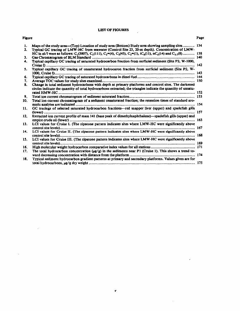
LIST OF FIGURES

Figure Page

1. Maps of the study area-(Top) Location of study area (Bottom) Study area showing sampling sites.. . . . . . . . . 134 2. Typical GC tracing of LMW-HC from seawater (Control Site 23, 20-m depth) . Concentration of LMW-

HC in nVl were as follows: C,(3807), 0(111), C2=(4), C3(43), C3=(1), iC4(11), nC4(14) and C5_7(8) .. . . . . . . . . 138 3. Gas Chromatogram of BLM Standard . . . . . . . . . . . . . . . . . . . . . . . . . . . . . . . . . . . . . . . . . . . . . . . . . . . . . . . . . . . . . . . . . . . . . . . . . . . . . . . . . . . . . . 140 4. Typical capillary GC tracing of saturated hydrocarbon fraction from surficial sediment (Site P2, W-1000,

Cruise I) . . . . . . . . . . . . . . . . . . . . . . . . . . . . . . . . . . . . . . . . . . . . . . . . . . . . . . . . . . . . . . . . . . . . . . . . . . . . . . . . . . . . . . . . . . . . . . . . . . . . . . . . . . . . . . . . . . . . . . . . . . . . 142 S. Typical capillary GC tracing of unsaturated hydrocaron fraction from surficial sediment (Site P2, W-

1000, Cruise I) .. . . . . . . . . . . . . . . . . . . . . . . . . . . . . . . . . . . . . . . . . . . . . . . . . . . . . . . . . . . . . . . . . . . . . . . . . . . . . . . . . . . . . . . . . . . . . . . . . . . . . . . . . . . . . . . . . . . . 143 6. Typical capillary GC tracing of saturated hydrocarbons in diesel fuel .. . . . . . . . . . . . . . . . . . . . . . . . . . . . . . . . . . . . . . . . . . . . . . . 144 7. Average TOC values for study sites examined... . . . . . . . . . . . . . . . . . . . . . . . . . . . . . . . . . . . . . . . . . . . . . . . . . . . . . . . . . . . . . . . . . . . . . . . . . . . 150 8. Change in total sediment hydrocarbons with depth at primary platforms and control sites. The darkened

circles indicate the quantity of total hydrocarbons extracted; the triangles indicate the quantity of unsatu- rated HMW-HC . . . . . . . . . . . . . . . . . . . . . . . . . . . . . . . . . . . . . . . . . . . . . . . . . . . . . . . . . . . . . . . . . . . . . . . . . . . . . . . . . . . . . . . . . . . . . . . . . . . . . . . . . . . . . . . . . . 152

9. Total ion current chromatogram of sediment saturated fraction.. . . . . . . . . . . . . . . . . . . . . . . . . . . . . . . . . . . . . . . . . . . . . . . . . . . . . . 153 10 . Total ion current chromatogram of a sediment unsaturated fraction; the retention times of standard aro-

matic analytes are indicated . . . . . . . . . . . . . . . . . . . . . . . . . . . . . . . . . . . . . . . . . . . . . . . . . . . . . . . . . . . . . . . . . . . . . . . . . . . . . . . . . . . . . . . . . . . .. . . . . . . . 154 11 . GC tracings of selected saturated hydrocarbon fractions-red snapper liver (upper) and spadefish gills

(lower) . . . . . . . . . . . . . . . . . . . . . . . . . . . . . . . . . . . . . . . . . . . . . . . . . . . . . . . . . . . . . . . . . . . . . . . . . . . . . . . . . . . . . . . . . . . . . . . . . . . . . . . . . . . . . . . . . . . . . . . . . . . . . . 157 12 . Extracted ion current profile of mass 141 (base peak of dimethylnaphthalene)-spadefish gills (upper) and

empire crude oil (lower) . . . . . . . . . . . . . . . . . . . . . . . . . . . . . . . . . . . . . . . . . . . . . . . . . . . . . . . . . . . . . . . . . . . . . . . . . . . . . . . . . . . . . . . . . . . . . . . . . . . . . . . . . 163 13 . LCI values for Cruise I. (The zipatone pattern indicates sites where LMW-HC were significantly above

control site levels).. . . . . . . . . . . . . . . . . . . . . . . . . . . . . . . . . . . . . . . . . . . . . . . . . . . . . . . . . . . . . . . . . . . . . . . . . . . . . . . . . . . . . . . . . . . . . . . . . . . . . . . . . . . . . . . . 167 14. LCI values for Cruise II . (The zipatone pattern indicates sites where LMW-HC were significantly above

control site levels). . . . . . . . . . . . . . . . . . . . . . . . . . . . . . . . . . . . . . . . . . . . . . . . . . . . . . . . . . . . . . . . . . . . . . . ., . . . . . . . . . . . . . . . . . . . . . . . . . . . . . . . . . . . . . . . . 168 15 . LCI values for Cruise III. (The zipatone pattern indicates sites where LMW-HC were significantly above

control site levels).. . . . . . . . . . . . . . . . . . . . . . . . . . . . . . . . . . . . . . . . . . . . . . . . . . . . . . . . . . . . . . . . . . . . . . . . . . . . . . . . . . . . . . . . . . . . . . . . . . . . . . . . . . . . . . . . 169 16 . High molecular weight hydrocarbon comparative index values for all stations . . . . . . . . . . . . . . . . . . . . . . . . . . . . . . . . . . . . . 171 17 . The total hydrocarbon concentration (ug/g) in the sediments near P1 (Cruise 1). This shows a trend to-

ward decreasing concentration with distance from the platform ... . . . . . . . . . . . . . . . . . . . . . . . . . . . . . . . . . . . . . . . . . . . . . . . . . . . . 174 18 . Typical sediment hydrocarbon gradient patterns at primary and secondary platforms. Values given are for

total hydrocarbons, FABIB dry weight . . . . . . . . . . . . . . . . . . . . . . . . . . . . . . . . . . . . . . . . . . . . . . . . . . . . . . . . . . . . . . . . . . . . . . . . . . . . . . . . . . . . . . . . . 175

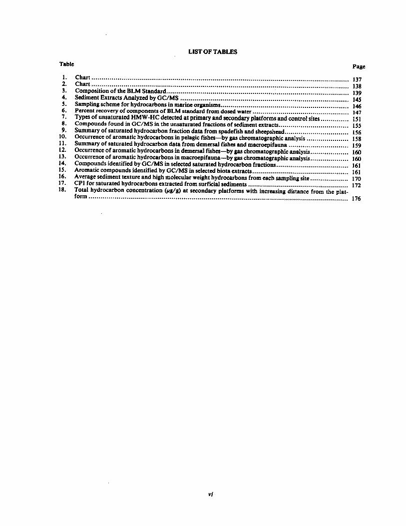
LIST OF TABLES

Table

1 . Chart . . . . . . . . . . . . . . . . . . . . . . . . . . . . . . . . . . . . . . . . . . . . . . . . . . . . . . . . . . . . . . . . . . . . . . . . . . . . . . . . . . . . . . . . . . . . . . . . . . . . . . . . . . . . . . . . . . . . . . . . . . . . . . . . 2 . Chart . . . . . . . . . . . . . . . . . . . . . . . . . . . . . . . . . . . . . . . . . . . . . . . . . . . . . . . . . . . . . . . . . . . . . . . . . . . . . . . . . . . . . . . . . . . . . . . . . . . . . . . . . . . . . . . . . . . . . . . . . . . . . . . . 3 . Composition of the BLM Standard. . . . . . . . . . . . . . . . . . . . . . . . . . . . . . . . . . . . . . . . . . . . . . . . . . . . . . . . . . . . . . . . . . . . . . . . . . . . . . . . . . . . . . . . . . . 4 . Sediment Extracts Analyzed by GC/MS . . . . . . . . . . . . . . . . . . . . . . . . . . . . . . . . . . . . . . . . . . . . . . . . . . . . . . . . . . . . . . . . . . . . . . . . . . . . . . . . . . . . S . Sampling scheme for hydrocarbons in marine organisms . . . . . . . . . . . . . . . . . . . . . . . . . . . . . . . . . . .��� , .���������� , 6 . Percent recovery of components of BLM standard from dosed water . . . . . . . . . . . . . . . . . . . . .� . . . . . . .��������� 7 . Types of unsaturated HMW-HC detected at primary and secondary platforms and control sites . . . . . . . . . . . . . . 8 . Compounds found in GC/MS in the unsaturated fractions of sediment extracts . . . . . . . . . . . . . . . . . . . . . . . . . ., .� . .� , 9 . Summary of saturated hydrocarbon fraction data from spadefish and sheepshead . . . . . . . . . . . . . . . . . . . . . . . . . . . . . . . . 10 . Occurrence of aromatic hydrocarbons in pelagic fishes-by gas chromatographic analysis . . . . . . . . . . . . . . . . . . . ., 11 . Summary of saturated hydrocarbon data from demersal fishes and macroepifauna . . . . . . . . . . . . . . ., . . . . . . ., . . . .� 12 . Occurrence of aromatic hydrocarbons in demersal fishes-by gas chromatographic analysis . . . . . . . . . . . . . . . . . . . 13 . Occurrence of aromatic hydrocarbons in macrcepifauna-by gas chromatographic analysis . . . . . . . . . . . . . . . . . ., 14. Compounds identified by GC/MS in selected saturated hydrocarbon fractions . . . . . . . . . . . . . . . . . . . . . . . . . . . . ���� 15 . Aromatic compounds identified by GC/MS in selected biota extracts . . . . . . . . . . . . . . . . . . . . . . . . .� , . . . . ., . ������ , 16 . Average sediment texture and high molecular weight hydrocarbons from each sampling site . . . . . . . . . . . . . . . . . . . 17 . CPI for saturated hydrocarbons extracted from surficial sediments . . . . . . . . . . . . . . . . . . . . . . . . . ., ., . . . .��� , . ���� , 18 . Total hydrocarbon concentration (Kg/g) at secondary platforms with increasing distance from the plat-

form ... . . . . . . . . . . . . . . . . . . . . . . . . . . . . . . . . . . . . . . . . . . . . . . . . . . . . . . . . . . . . . . . . . . . . . . . . . . . . . . . . . . . . . . . . . . . . . . . . . . . . . . . . . . . . . . . . . . . . . . . . . . . . . .

Page

137 138 139 145 146 147 151 155 156 158 159 160 160 161 161 170 172

176

vi

ABSTRACF

Samples taken at 20 production platform sites and four control sites is the north central Gulf of Mexico were ana-lyzed for low molecular weight hydrocarbons (LMW-HC)* in seawater, total organic carbon (TOG) and high molecu-lar weight hydrocarbons (HMW-HC) in sediments, and HMW-HC in invertebrates and fish. Analytical techniques in-cluded capillary column gas chromatography (GC), and capillary column gas chromatography/mass spectrometry (GC/MS). Results indicate that the whole of the Louisiana Outer Continental Shelf (OCS) study area is contaminated from chronic, low-level, multisource hydrocarbon pollution. High levels of LMW-HC were found in the water column anti are apparently associated with gas pipeline leaks. Levels of TOC in the sediments were not excessively high in com-parison to undeveloped areas of the Gulf OGS. Quantities of HMW-HC in sediments were variable and associated with site location relative to overall area production, Mississippi Rives influence, sediment drain size, and, in some in-stances, platform-related activities . Several platforms were indicated as probable sources of petrogenic hydrocarbons found in surrounding sediments. Low levels of aromatic hydrocarbons were found in 47% of the fauna samples; some samples -contained alkylated benzenes and naphthalenes which had isomer distributions similar to those seen in crude oil . No instances of massive contamination of sediments or fauna were seen .

" A glossary of abbreviations used in this report is liven in Appendix A.

V11

I . INTRODUCTION

A. Petroleum Hydrocarbons in the Marine Environ-ment Establishing the presence or absence of petroleum

contamination in the marine environment is important because petroleum hydrocarbons are toxic to marine ecosystems and certain of the aromatic constituents of oil are carcinogenic to man.

unsaturated fractions is useful as an indicator of the source of the hydrocarbons . Petroleum-derived hydrocarbons generally contain much higher quantities of unresolved components than do hydrocarbons from biogenic or pyro-genic sources (Youngblood and Blumer, 1975 ; Reed et al ., 1977) .

1. Sources of Hydrocarbons The terms biogenic, petrogenic, pyrogenic, and

anthropogenic are used to describe the sources of hydro-carbons . Biogenic hydrocarbons, produced by biologi-cal systems, include predominately odd-carbon number alkanes, pristane, and alkenes (e.g ., squalene) (Reed et al ., 1977) . Polycyclic aromatic hydrocarbons are not usually produced by biota in significant quantities . Pet-rogenic hydrocarbons are characterized by n-alkanes with no odd/even preference and a suite of aromatic compounds in which the alkylated homologues out-number the parent compounds (Blumer and Young-blood, 1975 ; Youngblood and Blumer, 1975 ; Reed et al ., 1977) . Pyrogenic hydrocarbons formed during com-bustion processes (e .g ., internal combustion engine, for-est fire) are characterized by unalkylated aromatics (Biumer, 1976 ; Hase and Hites, 1976) . Anthropogenic hydrocarbons are man-made and include many hydro-carbons also classed as pyrogenic and petrogenic .

2 . Indicators of Hydrocarbon Type An indication of the origin of a given suite of

high molecular weight hydrocarbons (C,4 C36) may be obtained by examining the data . The following indica-tors are important :

" A suite of alkanes may be characterized by de-termining its odd/even preference (OEP), a calculation to determine whether there is a preference for odd versus even carbon chain length . Petroleum hydrocarbons are indicated if there is no odd to even preference (Reed et al ., 1977) .

" A similar ratio is the carbon preference index (CPI) which is used to characterize a narrower range of alkanes (Bray and Evans, 1961) .

" The pristane/phyt8ne ratio is of interest be-cause pristane is a biogenic hydrocarbon whereas phytane is derived from petroleum (Meinschein, 1969 and National Academy of Sciences, 1975) . Similarly the pristane/n-C,7 and phytane/n-C~8 ratios may reflect the ori-gin of hydrocarbons .

" The presence of alkylated aromatic hydrocar-bons in amounts equal to or greater than the parent compounds is characteristic of petro-leum contamination (Youngblood and Blumer, 1975 ; Tissot and Welte, 1978) .

" An unresolved complex mixture (UCM) mani-fested by a rise in the baseline of a gas chroma-togram is due to many different hydrocarbons which are not separated from one another. The quantity of the UCM seen on the gas chro-matograms of both the saturated and

B. Other Studies in the Gulf of Mexico Some of the parameters examined in the present

study have been examined previously by Gulf Universi-ties Research Consortium (GURC) during the American Petroleum Institute (API) sponsored Offshore Ecology Investigation (OEI) (Lasater and Ledet, 1974 ; Ward, Bender, and Reish, 1979) . Evidence of petroleum con-tamination was found in the form of substantial unre-solved envelopes seen in many sediment samples and rel-atively high concentrations of n-paraffins present in Timbalier Bay (Morgan et al ., 1974) . No differences in total hydrocarbons were found between control and platform stations . Plankton and selected marine orga-nisms also showed evidence of contamination from petroleum-derived hydrocarbons . Many of the core sed-iment samples examined contained alkyl benzenes and naphthalenes similar to those seen in local crude oils . The OEI study concluded that although there was evi-dence of petroleum contamination, it was not of ecolog-ical significance (Ward et al ., 1979) .

Other important studies in the Gulf of Mexico in-clude two Bureau of Land Management (BLM) spon-sored programs : one offshore Mississippi, Alabama and Florida (MAFLA) (Dames and Moore, 1979) and the other on the South Texas Outer Continental Shelf (STOCS) (Parker, Scalan, and Winters, 1976, 1977, 1979) . Both studies provide background data for rela-tively unpolluted areas . In this report, data from these two studies are compared with data from the present study.

A recent effort off the coast of Texas is the Bucca-neer Gas/Oil Field Study (BGOF), sponsored by the En-vironmental Protection Agency (EPA) and conducted by the National Oceanographic and Atmospheric Ad-ministration (NOA.A) . This study is examining, among other things the contribution of hydrocarbons to the water, sediments, and biota during petroleum produc-tion activities (Middleditch and Basile, 1976, 1978, 1979 ; Middleditch ., Basile, and Chang, 1977, 1978, 1979 ; Middleditch and West, 1979) . Data from the BGOF study together with data from this study should provide a general picture of the impact of petroleum-related activities on the Gulf of Mexico .

C. The Central Gulf Platform Study

1. Study Area and Sampling Scheme Samples were collected in an approximately rect-

angular area west of the Mississippi Delta extending from 5 km (3 miles) to 115 km (69 miles) offshore and 225 km (135 miles) west (Fig . 1) . This area of the Louisi-ana Outer Continental Shelf (OCS) has been actively producing both oil[ and natural gas for more than 25 years .

133

105° 100° 95° 9p° 85° 80° 75°

35°

r.

30` San Antonio Houston New Orleans

~/U1/1/1~ Corpus Christi ~ STUDY AREA

Ft. Myars

25°

MEXICO ~nvna

CUB A

YUCATAN

SCALE

0 100 200 Nautical Miles

1 ~ i /U ~ ~ 1

9;e 3il, 96o '

AAarsh I . (/ G� a ? ,~.

+ oc m

~ w

r,

gay iy+ ` 0

ow c

: ~ ~ ~ a ~ r Pt . Au Far 1 . A t

~ 0°

X 21 5

Tarebonna k d Say 1 02

29° Timbalier Bay 121 '8 .

0 1 '8`

M

` 19 22

24 78 .~

" 20

"190" 7 " 9

r

.. cc,

' ~

~ _ o ~ .. . . .fl:_

___.__..__. .q

30' 1 6 23

17

15 PRIMARY SITES

~ SECONDARY SITES CONTROL SITES

m SCALE (kilometers)

"28° ' 0 10 20 30 40 oe

FIG. 1 . Maps of the study area-(Top) Location of study area (Bottom) Study area showing sampling sites .

134

Three cruises were made to include three cli-matic seasons : Cruise I, May 1978 ; Cruise II, August/ September 1978 ; and Cruise III, January 1979 . Four primary platforms (P1-P4) and four control sites (C21-C24) were samples during each cruise, Control sites selected to represent bottom types and depths similar to nearby study platforms were located in lease blocks where exploration and production had not occurred . Sixteen secondary platforms (SS-S20) were sampled only during Cruise II .

2. General Design of the Present Study This study was designed to monitor hydrocar-

bons in the water column, sediments, and marine biota . Low molecular weight hydrocarbons (LMW-HC) which include methane, ethane, ethene, propane, propene, n-butane, isobutane and a CS to C7 backflush peak were analyzed in the seawater column. The backflush peak also includes some low molecular weight aromatic com-pounds . The high molecular weight hydrocarbons (HMW-HC)(n-C]4 to rrC32, pristane, phytane, and se-lected aromatics) were analyzed in surficial and down-core sediments and biota . In addition, total organic car-bon (TOC) was determined in the sediments .

Analysis of downcore sediments was performed to provide an indication of the quantities of hydrocar-bons seen with depth . These data were to be correlated with lead-210 dating analysis in order to provide a time frame for the layered sediment and give an indication of hydrocarbon quantities in the sediment prior to explora-tion and production in this area . However, sediment turbation seems to preclude any downcore layering within the upper meter or so; this precluded any mean-ingful correlations .

The low molecular weight n-alkanes and aro-matic compounds (benzene, toluene and xylenes) have relatively high solubilities in seawater . Therefore, these compounds in the water column are excellent choices with which to study either a recent or on-going petro-leum input (oil spill, pipeline break, natural seep, etc .) into the seawater . The saturated n-alkanes in the range of C7-C14 have low solubility in water and evaporate rapidly from the water surface . Kreider (1971) has shown that, in a spill, all the hydrocarbons less than CAS (boiling point <250 C) will evaporate from the ocean water surface within 10 days . Therefore, these com-pounds would be included only in a study of a recent oil slick or sheen . Compounds of molecular weight greater than that of n-C14, because of their low volatility and their low solubility in the seawater, have a high proba-bility to either accumulate in the sediments or to form tar balls . Specific mechanisms in which petroleum hy-drocarbons may accumulate in the sediment are dis-cussed by the National Academy of Sciences (1975) .

Platforms studied varied according to age, de-gree of development, depth of water, sediment type, and production type (oil and/or gas) . The sites were selected to include all types of production platform environments .

3. Organic Chemistry Studies of Water and Sediments The purpose of this part of the organic chemical

analysis program was to establish levels of TOC in the sediments, of LMW-HC (CI -CQ) in the seawater, and of HMW-HC (n-C,4 to n-C32) in the surficial and

downcore sediments near production platforms on the central Gulf of Mexico OCS. Since these hydrocarbons may originate from spilled petroleum, data on their dis-tribution may reveal the impact of oil and gas explora-tion and development on the marine environment . Since these same organic materials may also originate from natural hydrocarbon seepages in the marine environ-ment, the data may also reveal the natural variations which might be expected on continental margins . The data would help establish the naturally-occurring varia-tions in these parameters as well as provide a basis for predicting the impact of oil and gas activities in frontier areas on and off the continental shelf .

a . Sediment TOC TOC in the sediments is a direct indicator of

the richness of organic productivity in the water col-umn, the degree of preservation, and the sediment type . Average TOC contents of recent sediments from the Gulf of Mexico have been reported to range from 0.5% (Hunt, 1961) to 0.9% (Philippi, 1965) . Occurrences of TOC significantly higher than these ranges combined with supportive data from HMW-HC analyses could in-dicate recent petroleum spills or natural seeps .

b . LMW-HCinSeawater Dissolved LMW-HC (methane, ethane,

ethene, propane, propene, isobutane, rrbutane and CS to C7 hydrocarbons) in the seawater are sensitive indica-tors of both petroleum and biological activity within a region (Sackett and Brooks, 1979) . Underwater venting of petroleum gases ;, gas pipeline leaks and natural gas seepages from the sediments contribute heavily to meth-ane, ethane, propane, isobutane, n-butane and CS to C7 hydrocarbon levels in the seawater . Biological activity also contributes dissolved methane as well as olefinic hydrocarbons (ethene and propene) to the water .

In a study by Swinnerton and Lamontagne, (1974), baseline measurements of LMW-HC were deter-mined in open ocean and nearshore water samples . A contamination index (CI) based on the average concen-trations of methane, ethane, and propane was proposed to differentiate between open-ocean clean water and water contaminated by hydrocarbons [CI = 1/3(C]/C-, + CZ/CZ + C3/C3 )] where 1 < C~ , CZ , and C3 are the average open ocean concentrations of methane, ethane, and propane respectively . Average values used in the calculation of CI were 49.5 nl/1 for methane, 0.50 nl/1 for ethane, and 0.34 nl/1 for propane . Based on concen-trations in the open. ocean, a CI greater than 5 indicates hydrocarbon contamination .

c. HMW-HCin Sediments The goat of this phase of the project was to

characterize HMW-HC (n-C,4 to n-C32) in the surficial sediments near production platforms and at control sites .

Typical values for hydrocarbon content of re-cent sediments in coastal basins, continental shelf and open marine basins are in the range of 20-100 1Ag/g (Tis-sot and Welte, 1978) . Recent sediments often contain saturated hydrocarbons characterized by o-alkanes that exhibit an odd carbon preference . Pristane and phytane contents are generally low compared to n-C,7 and n-C18, respectively ; high concentrations of pristane and phytane indicate petroleum contamination (Meinschein,

135

1969) . Hydrocarbons from ancient sediments and crude oils, in contrast, show no odd carbon preference and usually contain significant amounts of pristane and phytane .

Unsaturated hydrocarbons are commonly found in recent sediments (Palacas, Love and Gerrild, 1972; Youngblood and Blumer, 1975 ; Blumer, 1976 ; Reed et al ., 1977) . Establishing the origin of these unsat-urated compounds is often difficult . However, most authors agree that compounds such as pyrene and fluo-ranthene are products of high temperature formation (Blumer, 1976), such as by forest fire . Unsaturated hy-drocarbons in sediments are believed to be of petrogenic origin (Myers and Gunnerson, 1976 ; Reed et al ., 1977), if they contain :

" alkyl-substituted polynuclear aromatic hydro-carbons (PAH's)

" multiple isomers or homologous series of alkyl-substituted PAH's

" an unresolved complex mixture (UCM) of hy-drocarbons typical of weathered petroleum .

4. Hydrocarbons in Fauna

a . Background The purpose of this phase of the study was to

examine the tissues of ecologically and commercially important fishes and macroepifauna for contamination by petroleum hydrocarbons . Previous studies under controlled laboratory conditions and in natural environ-ments have provided ample evidence that marine ani-mals accumulate hydrocarbons from both pyrogenic and petrogenic sources (Lee, Sauerherber, and Benson, 1972 ; Pancirov and Brown, 1977 ; Bravo et al ., 1978 ; Middleditch et al ., 1979 ; Nunes and Benville, 1979) . This is of particular importance, not only because of the toxicity of hydrocarbons to marine ecosystems, but also because of the potential human health effects associated with consumption of contaminated tissues .

6 . Previous HMW-HC Analyses of Fauna from the Gulf of Mexico Data obtained from macroepifauna and

macronekton during the STOCS program showed that

very low levels of total hydrocarbons were present in the area, averaging two ppm or less with C,S and C,7 o-alkanes and pristane predominating . The odd carbon number preference, the low levels of phytane and the absence of aromatic hydrocarbons suggest that the area is free of petroleum contamination .

Results from the MAFLA study, completed in 1978, were similar to the STOCS results in that no evidence of petroleum contamination was found in the biota (Dames and Moore, 1979 ; Giam and Chan, 1979) .

Preliminary results from the BGOF study in-dicate that there is a low level of oil pollution through-out the area . Elevated aliphatic hydrocarbon levels were found in some of the fish, and pyrene and methylnaph-thalene were reported to be present in the biota (Middle-ditch and West, 1979) .

c. HMW-HC Analyses of Fauna in the Present Study The present study includes the examination

of hydrocarbons in macroepifauna and demersal and pelagic fish . Macroepifauna and demersal fish were se-lected to represent both non-motile and motile bottom dwelling biota . Pelagic fish are attracted by the plat-form structure and may accumulate certain platform-derived contaminants by feeding on fouling organisms, crustaceans, and other organisms associated with the platforms . Samples of several species of macroepifauna and demersal fish were collected at all stations (i .e ., platforms and control sites) while pelagic fish were col-lected only around platforms . Only the flesh from mac-roepifauna and demersal fish was examined, while seve-ral tissues of pelagic fish were examined including edible flesh, liver, and gonads or gills.

The analytical methodology for this program was designed to measure a selected number of aliphatic and aromatic hydrocarbons . The approach was to ex-tract the total hydrocarbons, separate them into two fractions, saturated and unsaturated, and analyze them by means of high resolution capillary GC using a flame ionization detector . A portion of the extracts was ana-lyzed by gas chromatography/mass spectometry (GC/MS) for confirmation of the identity of the hydro-carbons . The GC/MS efforts emphasized the unsatu-rated fraction because of its importance in discerning the presence or absence of petrogenic hydrocarbons .

136

Il . METHODS AND MATERIALS

A. Sediment TOC

1 . Sampling Methods Surficial sediment samples for TOC analysis

were obtained by subsampling Smith-McIntyre grabs (Kahlsico Model 214WA250) from primary and second-ary platforms and control sites . Samples for TOC analy-sis were taken from the first four Smith-McIntyre grabs at each site . A total of 140 samples was collected for analysis according to Table 1 .

Following drying, a measured scoop of iron and a measured scoop of copper initiator were placed in the crucible and the sample was burned in the Leco induction furnace in a one-liter-per-minute flow of purified oxy-gen . The carbon dioxide formed was absorbed on Asca-rite0 in a weighed absorption tube. The Leco instrument was fitted with an oversized Drierite0 purification tube in order to remove ; any excess water which might have formed . Sulfur dioxide, from any anhydrite present in the sample, was removed with manganese dioxide .

TABLE 1

Number of Number of Stations Samples

Cruise X Sites X per Site X per Station Total

I P1-P4 8. 1 32 C21-C24 1 1 4

II P 1-P4 8. 1 32 S5-S20 2"" 1 32 C21-C24 1 1 4

III P 1-P4 8' 1 32 C21-C24 1 1 - 4

'Stations at platforms were designated in meters on the four compass headings, i .e ., N, E, S, W at 500 and 2000 m

"" N-500, N-2000 m

Surficial sediments (uppermost 5 cm) of each Smith-McIntyre grab sample were subsampled using a 2-cm x 5-cm corer constructed of stainless steel and des-ignated for this purpose only . Subcores (>10 grams each) taken from the grab samples were pooled into a 40 g composite sample and stored in a clean hexane-rinsed glass container . The containers were sealed with aluminum foil-lined caps, labeled, logged and frozen . The corer was rinsed with seawater between sampling .

2. Laboratory Analyses The TOC was measured by combusting it to COZ

and determining the COZ gravimetrically on Ascarite0 . The procedure was as follows :

An aliquot of the sediment sample was oven dried at 75 C for ten hours . A small representative por-tion of this gross sample was ground by hand to a very fine particle size in an agate mortar and pestle . A weighed amount of the finely ground material was transferred into a Leco crucible in which it was dried at 75 C for an additional two hours . The crucible and con-tents were transferred into a specially designed vacuum filtration system and the ground sample cautiously acid-ified with two to three milliliters of cold 2N hydro-chloric acid . In samples where carbonates were present, and vigorous reaction took place, cold acid was added until the reaction abated . The cold hydrochloric acid was added very cautiously so that the reaction did not result in the loss of any of the sample from the crucible . Following initial acidification, the contents of the cruci-ble were treated with hot 2N hydrochloric acid at 60 C. On completion of the acidification, the liquid was fil-tered from the crucible by a vacuum suction and the contents thoroughly washed with distilled water to re-move any remaining traces of the acid . The crucible was then dried at 200 C for four hours .

At the beginning of each batch of organic carbon analyses, the instrument was calibrated by running rep-licate analyses on iron ring standards of varying organic carbon contents . The procedure was also performed with several empty crucibles in order to determine the crucible blank correction factor . During the analysis of sediment samples, every fifth sample was analyzed in duplicate .

Using these methods, the TOC levels normally found in surf icial sediments can be accurately measured to a detection limit of less than 1 part in 10,000 .

B. LMW-HC in Seawater

1. Sampling Methods Samples were obtained by sampling a hydrocast

using a series of 6 I GO-FLO (General Oceanics Model 1080) bottles lowered to sample just below the air-sea in-terface (approximately 1 m depth) and at 10 m intervals throughout the water column to within 10 m of the bot-tom . The near-bottom sampling depth was adjusted, where feasible, to sample any prominent "nepheloid layer." The depth observed for the presence of this layer was obtained by a transmissometer . The bottles were thoroughly washed with nitric acid and rinsed with distilled water prior to sampling in order to avoid contamination .

Upon retrieval of the hydrocast, a portion of the seawater in the GO-FLO bottle was decanted into a one-liter bottle until overfilled . Each bottle was then pre-served with sodium azide, capped with an aluminum foil-lined screw rap, sealed with tape, labeled, and shipped to the laboratory for analysis .

The sampling effort consisted of 40 profiles, one at each primary platform and control site during each cruise and one at each secondary platform during the

137

e, ct

nt4

C6' C7 ~1

C3"

i

FIG . 2. Typical GC tracing of LMW-HC from seawater (Control Site 23, 20-m depth) . Concentration of LMW-HC in nl/1 were as follows: C,(3807), C2(1 11), CZ=(4),

C,(43), C,=(1), iC,(11), nC,(14) and C,_,(8) .

Cruise II . A profile consisted of a minimum of one and a maximum of ten individual samples depending on the depth of the sampling station . A total of 136 samples was analyzed .

2 . Laboratory Analyses The originally proposed method of analysis

(Swinnerton and Linnenbom, 1967) required helium to be bubbled through the seawater and then collected in traps . However, during initial tests of test samples, the aluminum foil-lined caps which were used to seal the bottles in the field could not withstand any positive pressure and leaked freely when degasification proce-dures were attempted . Therefore, the method of analysis for LMW-HC was altered to follow that of

McAuliffe (1971) . Seawater (20 ml) was removed by sy-ringe and replaced by helium (20 ml) to create a head-space at atmospheric pressure . The sealed container was vigorously shaken for five minutes to strip the LMW-HC from the water . Then 8 ml of the headspace gas which was displaced by 8 ml of deionized degassed water was injected into a gas sampling valve with a 1 .0 ml standard loop . The sample then was valued into the Varian Model 1440 FID gas chromatograph equipped with a stainless steel column (3.2 mm X 2.40 m) packed with 100 mesh alumina . Figure 2 illustrates a typical GC tracing of the LMW-HC obtained in this study .

By this method methane, ethane, propane, pro-pene, isobutane, and n-butane were resolved and mea-sured by a digital integrator (Varian CDS-111) . The backflush peaks which contain predominantly CS-C., al-kanes, alkenes and/or low molecular weight aromatic hydrocarbons were also measured by the digital integra-tor, which was preprogrammed to adjust the slope sensi-tivity and peak width for that retention area . Although this method does not yield precise measurements of the CS-C., compounds (principally because one does not know the individual compounds and, therefore, does not know the flame response factor for the detector), the method does yield information on the presence of such compounds and a rough estimate of their concen-tration . The detection limit for the individual LMW-HC using these methods is about one part dissolved hydro-carbon in one hundred billion parts of seawater .

As an analytical check of the efficiency of the method to remove hydrocarbons from the samples, the headspaces of five samples were purged of all hydrocar-bons and the procedure was repeated . It was found that the first helium strip removed more than 90% of the LMW-HC from the water samples .

C. HMW-HC in Sediments

l. Sampling Methods

a. Surficial Sediments Surficial sediment samples for analysis of

HMW-HC were obtained by subsampling each of the first four Smith-McIntyre grabs collected at the desig-nated sampling sites . The total sampling effort was 220 samples taken as shown in Table 2 .

TABLE 2

Number of Number of Stations Samples

Cruise X Sites x per Site X per Station Total I P1-P4 16' 1 64

C21-C24 1 1 4 II PI-P4 8"" 1 32

S5-S20 4""* 1 64 C21-C24 1 1 4

III PI-P4 8** 1 32 C21-C24 1 1 4

All Quality Control Samples -16

"N,E,S,W at 100, 500, 1000 and 2000 m *"N,E,S, W at 500 and 2000 m """N at 100, 500, 1000 and 2000 m

138

Surficial sediment samples of each Smith-McIntyre grab were obtained by taking two subsamples from each of the grabs with a 5-cm diameter stainless steel corer to a depth of 5 cm. The two subsamples taken from the grab sample were combined into one sample and stored in a clean glass container. This container was sealed with an aluminum foil-lined cap, labeled, logged and frozen . Quality control samples were taken and processed in the same manner. The coring device was rinsed with seawater between samplings.

b. Downcore Sediments Samples were obtained as cores with a Kahl-

sico Piston corer (Kahlsico Model 217WA260) using a hexane-rinsed aluminum liner . They were collected at each primary platform (N-S00) and control site during Cruise I . A total of eight cores ranging in length from 20 to 52 cm were brought on board, capped, logged and frozen .

The intent of the coring operation was to col-lect samples at specific time/depth horizons . It was not possible to perform the time/depth study because when cores were analyzed for age with depth by lead-210 dat-ing they indicated complete mixing of the sediments throughout the length of the cores . However, the down-core sediments were analyzed for their hydrocarbon content at the intervals listed in Appendix B.4 to deter-mine the hydrocarbon profile as a function of depth .

c. Shipboard Contaminants Samples of fuel oil (diesel), engine oil, lute

oil, and bilge water from the research ship were col-lected to permit identification of any hydrocarbon con-tamination caused by shipboard activities . A total of eight samples were collected during Cruises I and III and analyzed for saturated and unsaturated hydrocar-bons . Gas chromatographic analyses of the petroleum hydrocarbons from these samples indicated characteris-tic chromatographic patterns . Sediment samples which contained putative petroleum contamination exhibited chromatograms which reflect weathered petroleum hy-drocarbons . There were no indications that shipboard hydrocarbons contaminated the samples .

2. Laboratory Analyses All extraction steps were carried out as described

in the following sections to obtain the saturated and un-saturated hydrocarbons from the samples prior to anal-ysis by GC and GC/MS.

All laboratory apparatus (glass, stainless steel or Teflon) that came in contact with the samples was cleaned rigorously shortly before use . A typical cleaning process involved soaking in No-Chromix0, rinsing with distilled deionized water, and successive rinsings with methanol, toluene and hexane . The procedure used for PyrexO glass was to clean the glassware with solvents, rinse thoroughly with deionized water, then bake at 480 C for 2 hours . All organic solvents used for cleaning glassware prior to sample preparation were analyzed by gas chromatography and their impurities measured .

A blank run analysis was conducted concurrently with sediment sample analysis (approximately one blank analysis for every twelfth sample) using identical meth-ods of extraction, column chromatography (CC), and GC, as described in the following sections . Although only glass-distilled solvents were used for extractions in

this study, SO ml of each solvent lot was concentrated by Kuderna-Danish concentrator and analyzed for possible contamination . The blanks and the solvent lots were free of contamination, indicating that the solvents, lab-oratory apparatus (glassware, rotaevaporators, etc .) and the analytical methods were satisfactory for trace hydrocarbon analysis .

The BLM standard and mixtures of standards consisting of saturated and unsaturated hydrocarbons were used regularly to evaluate recovery efficiency and column and gas chromatographic separations . The com-position of the BLM standard is given in Table 3 and a typical chromatogram of this mixture is shown in Fig . 3 .

TABLE 3 . Composition of the BLM Standard

Peak Concentration Number' Hydrocarbon (Exg/kl)

6 rrC1s 1 .0 8 o-C1b 1 .0 10 n-C17 0.5 11 pristane 1 .0 14 n-Ci8 0.1 15 phytane 0.1 16 n-C,9 0.1 19 n-C20: 1 0 .1 20 n-C20 0.1 13 o-C,8:, 0.1 22 n-CZ, 0.5 23 n-C22 0.1 ZS II-C26 0.1 26 n-C28 0.1 28 IJ-C30 0.1 29 n-C32 1 .5 27 cholestane (5 a) 0.5 18 androstane (5 a) 0.5 1 naphthalene 0.1 2 1-methylnaphthalene 1 .0 4 1,3-dimethylnaphthalene 1 .0 12 phenanthrene 0.1 17 3,6-dimethylphenanthrene 0.1 21 pyrene 0.1 9 9,10-dihydrophenanthrene 0.1 S acenaphthene 0.1 7 fluorene 0.1 3 biphenyl 0 .1

24 nonadecylbenzene 0.1 °see Figure 3

Recovery efficiency was evaluated by adding 200 lAg each of dimethylnaphthalene, pyrene and eicosane to a 2000-m1 round-bottomed flask containing toluene/ methanol (1 :1). The sample was then refluxed, ex- tracted, concentrated and chromatographed as de- scribed in the following sections . A set of five spiked tri- als was analyzed at the initiation of the project and a second set of five spiked trials was analyzed midway through the project. The results of these trials were as follows:

Mean % Number of Compound Recovery Trials Dimethylnaphthalene 63.9111 .2 10 Pyrene 91 .1 t 17.5 10 Eicosane 82.31 15.9 10

139

c

a V u b w O

a

2 4 6 >>

FIG . 3. Gas Chromatogram of BLM Standard

The level of separation of the BLM mixtures achieved by CC was typically less than 1 % of the unsat-urated compounds in the saturated hydrocarbon frac-tion and less than 1 % of each saturated hydrocarbon in the unsaturated fraction . Mass spectral searches of indi-cator compounds in the saturated and unsaturated frac-tions submitted for GC/MS analysis also indicated that the required separations by CC were obtained .

a . Sample Processing and Hydrocarbon Extrac-tion The surficial sediment samples were received

at the laboratory frozen at -5 C in glass jars . The down-core samples frozen at -5 C were removed from the alu-minum liner (5 .7 cm i.d .) by defrosting the outer part of the core in contact with the liner . The frozen core then easily slid from the liner onto a precleaned glass tray . The outer 2-4 mm of sediment were carefully scraped from the core with a stainless steel knife and discarded . The core was divided into sections consistent with the divisions made for lead-210 analysis . Sectioning infor-mation for specific samples can be found in Appendix B.4 . The same procedures for initial processing, reflux, CC and GC were employed on both surficial and down-core sediments .

The entire surficial sediment sample, was analyzed in most cases . Therefore, the samples did not require active homogenization .

The two primary methods of initially remov-ing water from the sediments are extracting the sediment with methanol and freeze drying the sample . Both of these methods were used in the STOCS study (Parker et al ., 1976, 1977 and 1979) . P.L . Parker (personal com-munication) stated that they observed no differences in the two methods but that he preferred the methanol pro-cedure over the freeze drying procedure because, in the methanol procedure, it is much easier to prevent con-tamination of the sample .

The sediment samples were refluxed with methanol for a minimum of 6 hours . This preliminary extraction removed water and possibly some of the hy-drocarbons . The remaining hydrocarbons were ex-tracted from the sample using toluene/methanol (1 :1) for at least 8 hours .

The extracts were recovered from the sol-vents by evaporation under partial vacuum in a flash evaporator at 46 C . Approximately 50 ml of a solution of potassium hydroxide in ethanol (30 g KOH per liter CZHSOH) were added for saponification . The mixture was refluxed on a steam bath for a minimum of 10 hours .

Distilled-deionized water was added to the saponified mixture and the non-saponifiable hydrocar-bons were extracted into hexane using a separatory fun-nel . They were mixed gently to avoid emulsion forma-tion . The hexane extract was then dried with anhydrous magnesium sulfate . Copper (powder, 4-5 g) was added prior to filtration of the extract to remove sulfur . The hexane was then evaporated from the extract using a Kuderna-Danish Evaporator. The final 4.0 ml were con-centrated under a nitrogen "blanket" at 40 C and the "total hydrocarbons" were recovered before all of the hexane was evaporated from the sample . Since the vapor pressure of hexane is significantly higher than tet-radecane at 40 C, the loss of compounds in the greater-than C I4 weight range was minimal .

b. CC Analysis The "total hydrocarbon" sample was sepa-

rated by CC into two fractions . A microcolumn (0.5 cm i.d . x 10.0 cm) was packed with silica gel (Bio-SiIOA, 100-200 mesh, Bio-Itad Laboratories), activated at 150 C for 6 hours, and pre-washed with purified hexane . The total non-saponifiable organic extract was washed onto the column with a small portion of hexane and the saturated hydrocarbons were eluted from the column with hexane (3-4 column volumes) . The unsaturated hy-drocarbons were eluted with 4 column volumes of 40% dichloromethane in hexane .

The eluting solvents were partially evapo-rated from the saturated and unsaturated hydrocarbons with a nitrogen stream at approximately 40 C to a vol-ume of about 0.2 ml .

c . GCAnalysis GC analysis was carried out on the fractions

eluted by CC. The fractions were separated on a glass capillary column (0.50 mm X 16 m) coated with OV-101 liquid phase (Scientific Glass Engineering, Inc .) . Rep-resentative GC tracings of a saturated and an unsatu-rated hydrocarbon fraction from surficial sediments, and a saturated fraction from diesel fuel are displayed in Figs . 4, 5, and 6, respectively . The high resolution, large loading capacity, and long-term stability of the OV-101 capillary column made it an excellent choice for detailed hydrocarbon analysis . The column was mounted in a flame ionization GC (Perkin-Elmer Model 3920-B) equipped with an all glass capillary injector, splitter, and detector . About 0.2 NI of sample was injected onto the capillary column . The following GC operating con-ditions were used :

Detector temperature Injection port temperature Temperature program Flow rate (at ambient temperature)

Split ratio

320 C 270 C 75 to 300 C at 16 C/min 2 ml/min He from column

25 ml/min He, make-up gas 30 ml/min HZ 300 ml/min air 30/l

The retention time and detector intensity of eluted compounds were measured by digital integrator (Varian CDS-111) and recorded on a strip chart . Areas of major peaks were calculated by the electronic integra-tor and graphically checked by the operator . In cases where near-baseline separation was not possible, areas were remeasured by calculating height times width at 1/2 height . The complex mixture of compounds ob-tained in these fractions was partly resolved by high res-olution GC . An unresolved envelope of compounds other than n-alkanes and isoprenoids was often found .

Quantitative measurements of individual compounds were made by comparing the peaks to the internal standard (Dlo anthracene) . This internal stan-dard has a retention time between pristane and C18 in the saturated fraction and immediately after phenan-threne in the unsaturated fraction . The detection limit for the individual hydrocarbons using these methods is one part hydrocarbon in ten billion parts surficial sediment .

141

N

n

Ef

V1

Fi O

~

A C7

O

i -~ cn

PR/STAKE

~ /N

TERNAL

STAN

DARD

C18

~ PNYTANE

C/9

CPO

1 CZ/

CPP

CP3

CPS

o

-----

CY3

\ ~ a

cm

,cps

O

Ct9

1 ~ o

~C29

I ^

C so

Ito

C3/

--

I

1~

I .

I

t

h

W I , V 2

1

Y I I UNRESOLVED COMPLEX

AI/XTURE

i

,r---- -------/ oASEG/NE

100, i

FIG. S. Typical capillary GC tracing of unsaturated hydrocarbon fraction from surficial sediment (Site P2, W-1000, Cruise I) .

143

~n

.. n

o~

d. GC/MS Forty-two sediment extracts were analyzed

by GC/MS (Table 4) . The extracts were stored in sealed ampules at 4 C until analyzed . The compounds searched for in the saturated fraction included the n-alkanes (C�-C,), pristane and phytane whereas the unsaturated fractions were scanned for a variety of aromatic compounds (see Table 8) . Since the unsaturated extracts were so complex, components were located by the single ion monitor technique.

GC/MS analyses were performed on a Finni-gan Model 3300F equipped with a Grob-type split-split-less capillary column injector. The GC column and op-erating conditions for GC/MS analysis were the same as

TABLE 4. Sediment Extracts Analyzed by GC/MS

Saturated Fractions Cruise I

Cruise II

Cruise III

P3 P4 P4 P4 P2 S12 S12 S15 C23 P2

west 1000 north 100 north 1000 south 100 west 2000 north 100 north 2000 north 1000 (Control) north 500

Unsaturated Fractions Cruise I

Cruise II

Cruise III

PI P1 P1 P2 P3 P3 P3 P3 P4 P4 P4 C21 P1 P2 P3 P3 P3 P3 SS S7 S8 S12 S12 S15 S15 S16 S17 S17 S18 C21 C22 P1 P2

north 1000 east 100 east 2000 south 100 east 2000 south 100 south 1000 west 1000 east 100 south 1000 west 1000 (Control) west 500 east 500 east 2000 south 2000 west 500 west 2000 north 500 north 1000 north 100 north 500 north 2000 north 500 north 500 north 2000 north 500 north 1000 north 100 (Control) (Control) north 2000 north 500 north 500

those described for the GC analyses except that the tem-perature program was 10 C/min. The MS operating conditions were as follows :

Ionization voltage 70 eV Ion source temperature 80 C Mass range 50-500 amu Scan time 1 sec Integration time 2 msec

The performance of the GC/MS was checked daily by injecting the BLM standard (See Table 3, Fig . 3) and by introducing decafluorotriphenylphosphine (DFTPP) via the leak inlet . Instrument performance was considered acceptable if :

(a) n-C,7 was resolved from pristane and n-C,8 was resolved from phytane,

(b)the normal alkanes, C14 through C3Z, were resolved,

(c) the standard peaks were nearly symmetrical in shape; and

(d) if the DFTPP spectrum met the criteria set by Eichelberger, Harris, and Budde et al ., 1975 .

Compound identifications were based on comparison to the retention index and mass spectrum obtained from an authentic standard . Occasionally, ten-tative identifications were made, based on comparison to library spectra .

D. Hydrocarbons in Fauna

1 . Sampling and Shipboard Processing Macroepifauna and demersal fish were collected

with a 9-m (30-ft .) otter trawl . Trawl nets, made of un-coated nylon, were towed in the vicinity of each sam-pling site, retrieved,, and contents emptied into stainless steel dump trays . The nets were cleaned frequently by towing at depth with the cod end open . Platform-associated fish were obtained either by angling or spear-ing . The sampling scheme outlined in Table 5 was fol-lowed when possible . Emphasis was placed on obtaining the following organisms : 1) shrimps (Penaeus aztecus and P. setiferus) and oysters (Crassostrea and Ostrea spp .) to represent macroepifauna, 2) spadefish (Chaeto-dipterus faber), sheepshead (Archosargus probatoce-phalus) and red snapper (Lutjanus campechanus) to represent pelagic fishes, and 3) Atlantic croaker (Micro-pogon undulatus) to represent demersal fishes . Hexane-rinsed stainless steel utensils (tongs, trays, etc .) and hexane-rinsed rubber gloves were used for all onboard handling of samples . Organisms were either wrapped in hexane-rinsed aluminum foil or placed in hexane-rinsed metal cans and frozen .

The terms pelagic and demersal are used here in an operational sense, e.g ., Atlantic croaker obtained during trawls away from the platform were designated demersal while these occasionally angled at the plat-forms, although not the species sought, were taken as the best available and labeled pelagic . The latter croak-ers were larger and probably farther up the food chain in preferred prey; therefore, the pelagic designation may be comparable to other species taken as pelagic .

145

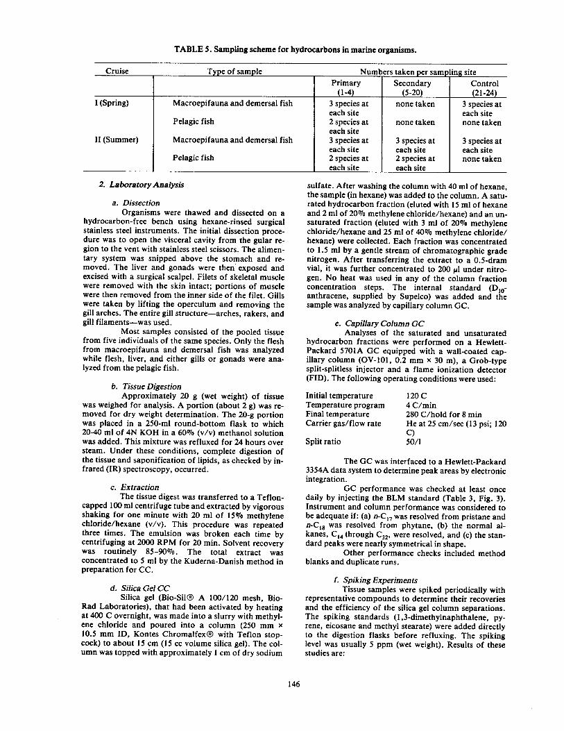
TABLE S. Sampling scheme for hydrocarbons in marine organisms.

c;ruise 1 e of sample Numbers taken per sam lin site Primary Secondary Control

1-4 5-20 21-24 I (Spring) Macroepifauna and demersal fish 3 species at none taken 3 species at

each site each site Pelagic fish 2 species at none taken none taken

each site II (Summer) Macroepifauna and demersal fish 3 species at 3 species at 3 species at

each site each site each site Pelagic fish 2 species at 2 species at none taken

each site each site

2. Laboratory Analysis

a . Dissection Organisms were thawed and dissected on a

hydrocarbon-free bench using hexane-rinsed surgical stainless steel instruments . The initial dissection proce-dure was to open the visceral cavity from the gular re-gion to the vent with stainless steel scissors . The alimen-tary system was snipped above the stomach and re-moved . The liver and gonads were then exposed and excised with a surgical scalpel . Filets of skeletal muscle were removed with the skin intact; portions of muscle were then removed from the inner side of the filet . Gills were taken by lifting the operculum and removing the gill arches . The entire gill structure-arches, rakers, and gill filaments-was used .

Most samples consisted of the pooled tissue from five individuals of the same species . Only the flesh from macroepifauna and demersal fish was analyzed while flesh, liver, and either gills or gonads were ana-lyzed from the pelagic fish .

b. Tissue Digestion Approximately 20 g (wet weight) of tissue

was weighed for analysis . A portion (about 2 g) was re-moved for dry weight determination . The 20-g portion was placed in a 250-m1 round-bottom flask to which 20-40 ml of 4N KOH in a 60% (v/v) methanol solution was added . This mixture was refluxed for 24 hours over steam . Under these conditions, complete digestion of the tissue and saponification of lipids, as checked by in-frared (IR) spectroscopy, occurred .

c. Extraction The tissue digest was transferred to a Teflon-

capped 100 ml centrifuge tube and extracted by vigorous shaking for one minute with 20 ml of 15% methylene chloride/hexane (v/v) . This procedure was repeated three times . The emulsion was broken each time by centrifuging at 2000 RPM for 20 min . Solvent recovery was routinely 85-90%. The total extract was concentrated to 5 ml by the Kuderna-Danish method in preparation for CC .

d. Silica Gel CC Silica gel (Bio-Silo A 100/120 mesh, Bio-

Rad Laboratories), that had been activated by heating at 400 C overnight, was made into a slurry with methyl-ene chloride and poured into a column (250 mm x 10.5 mm ID, Kontes Chromalfex0 with Teflon stop-cock) to about 15 cm (15 cc volume silica gel) . The col-umn was topped with approximately 1 cm of dry sodium

sulfate . After washing the column with 40 ml of hexane, the sample (in hexane) was added to the column . A satu-rated hydrocarbon fraction (eluted with 15 ml of hexane and 2 ml of 20% methylene chloride/hexane) and an un-saturated fraction (eluted with 3 ml of 20% methylene chloride/hexane and 25 ml of 40% methylene chloride/ hexane) were collected . Each fraction was concentrated to 1 .5 ml by a gentle stream of chromatographic grade nitrogen . After transferring the extract to a 0.5-dram vial, it was further concentrated to 200 yl under nitro-gen . No heat was used in any of the column fraction concentration steps . The internal standard (D10-anthracene, supplied by Supelco) was added and the sample was analyzed by capillary column GC.

e. Capillary Column GC Analyses of the saturated and unsaturated

hydrocarbon fractions were performed on a Hewlett-Packard 5701A GC equipped with a wall-coated cap-illary column (OV-101, 0.2 mm X 30 m), a Grob-type split-splitless injector and a flame ionization detector (FID) . The following operating conditions were used :

Initial temperature Temperature program Final temperature Carrier gas/flow rate

Split ratio

120 C 4 C/min 280 C/hold for 8 min Heat 25 cm/sec (13 psi ; 120 C) 50/1

The GC was interfaced to a Hewlett-Packard 3354A data system to determine peak areas by electronic integration .

GC performance was checked at least once daily by injecting the BLM standard (Table 3, Fig . 3) . Instrument and column performance was considered to be adequate if : (a) n-C17 was resolved from pristane and n-C,8 was resolved from phytane, (b) the normal al-kanes, C14 through C3Z, were resolved, and (c) the stan-dard peaks were nearly symmetrical in shape .

Other performance checks included method blanks and duplicate runs .

f. Spiking Experiments Tissue samples were spiked periodically with

representative compounds to determine their recoveries and the efficiency of the silica gel column separations . The spiking standards (1,3-dimethylnaphthalene, py-rene, eicosane and methyl stearate) were added directly to the digestion flasks before refluxing . The spiking level was usually 5 ppm (wet weight) . Results of these studies are :

146

Mean % Number of Compound Recover Trials Dimethylnaphthalene 62.4±14.7 33 Pyrene 95.8123.6 35 Eicosane 79.8124.4 40

The efficacy of the silica gel column separa-tion was tested by dosing the GC standard into water and processing the spiked water as if it were a sample

(i .e ., digestion, extraction, concentration and silica gel CC). The saturated and unsaturated fractions were ana-lyzed in the same fashion as the samples and the percent recoveries were determined (Table 6) .

g. GC/MS Analyses of tissue extracts by GC/MS were

performed in the same manner as described previously for sediment analyses except that the GC temperature program was 4 C/minute .

TABLE 6. Percent recovery of components of BLM standard from dosed water

Saturated Fraction Unsaturated Fraction

Compound Recover Compound Recover n-C,4 80 napthalene 70 o-C,s 83 1-methylnaphthalene 73 n-C,6 84 biphenyl 76 n-C,7 83 1,3-dimethylnaphthalene 75 o-C,B 83 acenaphthalene 76 o-C,,:2 83 fluorene 80 phytane 87 phenanthrene 80 pristane 86 9,10-dihydrophenanthrene 81 o-C1y 88 3,6-dimethylphenanthrene 91 androstane(Sa) 87 pyrene 90 o-C20 88 nonadecylbenzene 61 n-C20 : 1 84 o-C2, 89 rt-C22 89 nonadecylbenzene 35 o-C26 99 cholestane(S a) 101 n-C29 102 o-C3o 99 o-C32 98

147

III. RESULTS

Detailed results of the organic chemical analyses of seawater, sediment, and fauna are tabulated in the data summary volume (Volume I, Part 8) . A summary of data for LMW-HC in seawater and TOC and HMW-HC in sediment is presented in Appendix B .

A. Sediment TOC Average TOC values for each study site are dis-

played in Fig . 7 (sites containing the highest concentra-tions of organic carbon are illustrated by a "zipatone" pattern for ease of visualization) . The TOC of surficial sediment samples is tabulated in Appendix B.1 . The average TOC for all primary platforms and control sites did not change appreciably during the three sampling seasons (I, 0.63 ; II, 0.53 ; III, 0.63%) .

Relatively high average TOC values (greater than 0.80%) were found in the sediments from Platforms S6, S7, S9, and 513 . These platform sites are grouped within 25 km of each other and near the Southwest Pass outflow of the Mississippi River . Surficial sediments from Platform S13 had the highest average TOC con-tent (1 .08%) . Only one other site, S10 (0.85%), had an average TOC value greater than 0.80% . Figure 1 and background information on currents indicate that the Mississippi obviously contributes most of this TOC.

The average TOC values for the sediments from Platforms P2 and P3 were consistently lower than those from the other primary sites and the control sites . The lowest average TOC value (0.11%) was found at S19 . Sediments from this site are mostly sand with minor amounts of silt and clay . Organic detritus is usually poorly preserved in large-grained sediments .

B. LMW-HC in Seawater Methane concentrations in seawater collected during

Cruise I were highest at Control Site C23 (3810 nl/1 at 20 m) . This sample also had the highest concentrations of ethane, propane, n-butane and isobutane of any sam-ples from Cruise I . The methane levels in Cruise I sam-ples were highest at the intermediate depths (10 and 20 meters) at all sites . This stratification was also detected in several samples collected during Cruises II and III . Two examples of this phenomenon were encountered at S16 and C23 during Cruise II when the methane levels (in nl/1) were as follows :

Depth m Site S16 Site C23 0 2,730 297 10 23,900 1,420 20 11,500 1,750 30 2,940 558 40 2,210

The highest concentrations of methane were found in samples from Cruise II . The primary sites and control sites had nearly twice the average methane compared to methane values from the other two cruises . Seawater from Secondary Platforms S8 and S16 had 22,400 and 23,900 nl/1 of methane, respectively, at 10 meter depths. These samples also contained significantly high levels of CZ C4 saturated hydrocarbons (ethane, propane, isobu-tane, and o-butane) .

The highest concentrations of ethene and propene were also found during Cruise II . Platforms P2, S8, and 512, which are within 17 km of each other and within 25 km of shore, had relatively high values of ethene (18 .1, 25.2 and 17.6 nl/1, respectively) . Only trace amounts of unsaturated LMW-HC were detected in the 22 samples collected during Cruise III .

Methane content in seawater samples collected at the Control Sites during Cruise III decreased significantly to an average of 604 nl/1 . However, the methane levels at the primary sites remained high at 1760 nl/1 .

C. HMW-HC in Sediments HMW-HC (C14-F) were detected in sediments from

all sites . Typical GC patterns of saturated hydrocarbon fractions contained o-C,4 to n-C32, pristane, phytane and an unresolved envelope of compounds . An odd-carbon preference of n-alkanes which is most distinct between C24 and C,,2 was the most frequently observed pattern . The unsaturated hydrocarbon fractions most often contained naphthalene, pyrene, chrysene and/or benzo(a)pyrene along with a relatively large amount of polyunsaturated hydrocarbons .

1. Surficial Sediments

a . Total Hydrocarbons The total. hydrocarbons which were extracted

from the surficial sediments ranged from a high concen-tration (average for platform) of 87 .4 jAg/g at S6 to a low of 5.7 ;Ag/g at S19 (Appendix B.3 .) .

Samples from P 1, S6, S 11, S 13, and S 16 were determined to contain high total hydrocarbon content in the sediments relative to the Control Sites . Total hydro-carbon content decreased with distance from the plat-form at S11 (220 Ng/g at 100 m, 10 Mg/g at 500 m, 6 Ng/g at 1000 m and 13 ;Ag/g at 2000 m).

The primary and secondary platforms with average HMW-HC concentrations that were less than the average value for the control sites (35 .1 jAg/g) were P2, P3, P4, S5, S9, S10, 512, 514, S15, S19, and S20 .

In most samples the bulk of HMW-HC con-sisted of an unresolved complex mixture (UCM) of com-pounds which was observed in the chromatograms of both the saturated and unsaturated hydrocarbon frac-tions . The average UCM for all samples was 96.4% of the total hydrocarbons .

b . Saturated Hydrocarbons The average concentration of the saturated

hydrocarbon fraction was 22.1 jAg/g and ranged from a high of 316 jAg/g to a low of 0.82 NgYg . The three sam-ples which contained more than 100 pg/g of saturated hydrocarbons (all from P1) had gas chromatograms which were dominated by UCM.

The n-alkane content predominantly had an odd-to-even carbon preference . The carbon range of n-C24 to o-C3Z had the strongest odd-carbon preference .

Pristane and phytane were detected in nearly all of the sediments . The average ratio of pristane to phytane for all cruises was 1 .15 ; pristane to n-C17, 1 .09 ; and phytane to o-C~B, 0.67 .

149

WEST COT[ i __ YT

FRANKLIN

IIOp3AN CITY fv

NOU MA

f

arc ) ~'Ve~Y. ' 1

BAR"TAqIA

010

GOLDEN MEADOW

U O

14

, . 17

PL ~�, ~ J1~ /1j ~J V MI /FR l. a

\ VENICE\ 21

" GRAND % ISLE

TERRENOMME SAY

. . . . . . . .

040, 0, 2 cap. 12

a 13 6

24 X90 10 I22

.T ~ 2

9 ..

t` ' 3 -- j ~ . . . . . . .. . . . ... .. . . . . .. . : : -- SCALE

16 ' DIAMETER OF CIRCLE

0.00 WT

. - 0.50

. 15 SCALE 'I , ."' O 1 2 3 4.

1 00 or > .

FIG. 7. Average TOC values for study sites examined .

c. Unsaturated Hydrocarbons Unsaturated hydrocarbons were found at all

platform sites . Typical unsaturated hydrocarbon GC patterns indicated an extensive mixture of aromatic and polyunsaturated hydrocarbons which often resulted in an unresolved envelope . GC analyses indicated the pres-ence of both pyrogenic and petrogenic aromatic hydro-carbons in all the sediments . Table 7 illustrates the presence/absence of several monitored compounds at each platform site . This table gives the combined find-ings of multiple samplings at each site. Unsaturated hy-drocarbon fractions from sediments which yielded GC tracings with abundant (>30 ppm) UCMs were found at P1, S6, S11, S13, and S16 .

Surficial sediments near P1 contained an un-usually wide array of unsaturated compounds. These sediments typically contained a UMC, pyrogenic aro-matic hydrocarbons (pyrene and fluoranthene), petro-genic aromatic hydrocarbons (naphthalene and isomers of dimethylnaphthalene and dimethylphenanthrene) and anthropogenic compounds (polychlorinated biphe-nyls and phenoxybiphenyls) . Total unsaturated hydro-carbons at P 1 averaged 34.9 ppm with the highest value, 364 ppm, at 100 m south of the platform .

2. Downcore Sediments The cores from the primary platforms and con-

trol sites were from 20 to 52 cm long (Appendix B.4 .) . Each core was divided into a minimum of three intervals according to depth . In three cases, additional cuts were made either because of the extra length of the core or because the core fractured during removal from the alu-minum core-liner .

There was an increase in the total hydrocarbons with depth of core at all sites (Fig . 8) . In each case (ex-cept at Site C24) the section with the highest amount of extractable hydrocarbons was the lowest interval .

a. Saturated Fraction The GC patterns of the saturated fractions

from the downcore samples indicated a predominant odd-to-even carbon preference . The carbon range of n-C24 to n-C32 had the strongest odd-carbon preference .

Pristane and phytane were detected in all samples . The average pristane to phytane ratio was 0.76 .

The results of the GC/MS analyses of the sat-urated fraction were in good agreement with those ob-tained in the GC analyses, i .e ., the compounds reported to be present by GC retention time were confirmed by GC/MS and the quantities were found to be similar . An example of a total ion current (TIC) chromatogram of a sediment saturated fraction is presented in Fig . 9.

b. Unsaturated Fraction The unsaturated hydrocarbon GC patterns

indicated an extensive mixture of aromatic and polyun-saturated hydrocarbons which often resulted in an unre-solved envelope .

The pyrogenic compounds, fluoranthene, pyrene and benzo(a)pyrene were found in every unsatu-rated extract . Other frequently occurring compounds were perylene (27 times), phenanthrene (24 times), dimethylphenanthrene (22 times) and naphthalene (15 times) . A complete list of the unsaturates found in all sediment extracts analyzed by GC/MS is given in Table 8 . These compounds rarely gave discrete TIC peaks . It can be seen in the sediment unsaturated fraction TIC chromatogram shown in Fig . 10 that the aromatic con-stituents found by single ion monitoring were either bur-ied in the UCM or masked by much larger nearly co-eluting peaks which were determined to be polyunsatu-rated aliphatic hydrocarbons . A consequence of this finding is that the aromatic components in the sediment extracts cannot be quantified by flame ionization GC . Moreover, it is doubtful that a reliable qualitative pro-file can be generated by the GC approach taken in this study .

D. Hydrocarbons in Fauna The results of the GC analyses of n-alkanes and se-

lected unsaturated and aromatic hydrocarbons are tab-ulated in Volume I, Part 8 . Individual tissue concentra-tions (jAg/g wet weight) of the compounds in the BLM standard (Table 3) and squalene are given for selected tissues of pelagic fishes, and for the flesh of demersal

TABLE 7. Types of unsaturated HMW-HC detected at primary and secondary platforms and control sites

COMPOUNDS

naphthalene 1-methylnaphthalene biphenyl 1,3-dimethylnaphthalene acenaphthene fluorene 9,10-dihydrophenanthrene phenanthrcne 3,6-dimethylphenanthrene fluoranthene pyrene chrysene/triphenylene nonadecylbenzene perylene/3,4-benzpyrene phenoxy biphenyls' polychlorinated biphenyls'

1 2 3 4 5 6 7V 8 v 9 10 11 12 13 14 15 16 17 18 19 20 21 22 23 24 + + " + 0 + " + + " + " 0 + + + " + +

" + " + + + i i + + + + + + ' + i + + + + ' + + + + ' + + + " + + 0 + + + 0 + 0 . 0 + + + + + + i + ' + + + i + + + + + + + " + ' + + + + " + + " + + + + + + + + + + + + + + + + + 0 + + + + +

i + + + + + " + + + + + + + + + + + + + + + + 0

+ + i + + + + i + + i 0 i + + + " " + +

+ " ' + + + " + + ' + " + + + ' " + +

i i i i i + i i + + + i + + i i i ' + + i i + + 0 0 0 0 0 0 0 0 p " " 0 0 0 0 0 . 0 0 0 0 . 0 0 0 0

0 Not detected f Detected by GC retention time " Confirmed present by GC/MS i Confirmed present by GC/MS and isomers detected 1 Searched for only by GC/MS, not monitored by GC .

151

0

io

x d 030

40

PI P2

~ 20

50

U N O

10

E 20

x f-a 0 30

40

so 0

P3 P4

s

C22 C23 C24

1 V ZU 30Aq/9 0 10 20 30,uq/q 0 10 20 30y919 0 10 20 30yu9/2

FIG. 8. Change in total sediment hydrocarbons with depth at primary platforms and control sites. The darkened circles indicate the quantity of total hydrocarbons extracted; the triangles indicate the quantity of unsaturated HMW-HC.

w

100

i c c y

U ti

FIG. 9. Total ion current chromatogram of sediment saturated fraction .

t

L

ra

pyrene 0 rn fluoranthene

dimethylpheaanthrene --~

m

anthracene ~ m

phenanthrene

N n

O ~~~p,~-, N 'n

benzMa)PYrene

o 0 naphthalene

F

p Crhry$rrde -sE S l.

G b "r e

FIG. 10. Total ion current chromatogram of a sediment unsaturated fraction; the retention times of standard aromatic analytes are indicated .

154

TABLE 8. Compounds found by GC/MS in the unsaturated fractions of sediment extracts.

Number of Compound Occurrences

naphthalene 15 methylnaphthalenes 8 biphenyl 3 dimethylnaphthalenes 9 acenaphthene 1 fluorene 4 9,10-dihydrophenanthrene 3 phenanthrene 24 dimethyl and ethyl phenanthrenes/

anthracenes 22 fluoranthene 32 pyrene 32 chrysene/triphenylene/benzanthracene 28 perylene 27 benzo(a)pyrene 32 dibenzochrysene/indenopyrene/

benzoperylene 14 dibenzanthracene/benzo(b)chrysene 3 polychlorinated biphenyls 0 2,2-bis-(p-chlorophenyl)-

1,1-dichloroethylene 1

fishes and macroepifauna . In addition, the ratios of phytane/CAB, pristane/C1.� and pristane/phytane, the percent (C,s + Cl7) and carbon preference indices are listed .

1 . Pelagic Fish Since the majority (30 samples out of 45) of pe-

lagic fish analyzed were either sheepshead or spadefish, data obtained from these species are emphasized .

a . Saturated Fraction The concentrations of total n-alkanes, pris-

tane and phytane, the CPI and the pristane-phytane ra-tios found in spadefish and sheepshead are given in Table 9 . Representative GC tracings of the saturated fraction obtained from spadefish and red snapper are shown in Fig . 11 . The n-alkane levels in spadefish and sheepshead demonstrate a consistent relationship with tissue type, i .e ., the lowest concentration of n-alkanes occurred in flesh while the highest concentrations were found in liver . This trend was found in most species of pelagic fish analyzed . The most frequently occurring n-alkanes in pelagic fish were pentadecane and heptade-cane. Pristane was detected in 71, 79, and 74% of flesh, gill and liver samples, respectively . Flesh samples con-tained the lowest levels of pristane while the highest con-centrations were found in either gills (sheepshead) or liver (spadefish) . Phytane occurred in far fewer samples (16, 38 and 28% of flesh, gills and liver, respectively) and at much lower levels than pristane . Only four in-stances in which the level of phytane exceeded 100 ppb (wet weight) in pelagic fish tissue were recorded . The pristane/phytane ratio was greater than unity in all but two cases . No instances of UCM were found in the satu-rated fractions .

b. Unsaturated rraction Forty percent (51 out of 129) of the unsatu-

rated fractions obtained from pelagic fish tissues gave a

positive GC response at the retention time for at least one of the aromatic compounds in the BLM standard . These data are summarized in Table 10 . The most fre-quently found aromatic materials were pyrene (19 times), 1,3-dimethylnaphthalenes (16 times) and 1-methylnaphthalene (14 times) . Squalene, a naturally-occurring intermediate in steroid biosynthesis, was found in high concentrations in most aromatic fractions .

2. Demersal Fish and Macroepifauna Eleven species of demersal fishes and twelve

species of macroepifauna were analyzed . The species most frequently analyzed were Micropogon undulatus (Atlantic croaker), sampled nine times, and Penaeus az-tecus(brown shrimp) obtained at 13 sites .

a. Saturated Fraction A summary of all demersal fish and macroe-

pifauna saturated traction data is presented in Table 11 . Total n-alkane levels for Atlantic croaker and brown shrimp (range 0 to 22 ppb) are somewhat lower than those found in the pelagic fish . Again, the most fre-quently found o-alkanes were pentadecane and heptade-cane and no UCMs were encountered . Pristane was found in approximately 71 % of the samples analyzed . Generally, pristane levels were higher in organisms showing the higher o-alkane concentrations . Phytane was found in 31 % of the samples ; however, it never ex-ceeded 20 ppb (wet weight) .

b . Unsaturated Fraction Capillary GC analysis indicated the presence

of aromatic components in eight of 19 demersal fish samples and in 10 of 31 samples of macroepifauna (Tables 12 and 13, respectively) . Methylnaphthalene (seven times), 1-methylnaphthalene (six times), and 1,3-dimethyl-naphthalene (five times) were found most often . The concentration range observed for these com-pounds in all but one sample was 10-220 ppb (wet weight) ; however, the majority of samples showed less than 70 ppb .

High levels (1-5 ppm, wet weight) of squalene were found in most samples of demersal fish ; the mac-roepifauna contained lower levels . It is noted that the four demersal fish samples caught at Control Site 21 ex-hibited levels of squalene ten times greater (in the 50 ppm, wet weight range) than those observed at other sites .

3. GC/MS Analyses Analysis of 47 fractions (7 saturated and 40 un-

saturated) by capillary column GC/MS was done both to confirm GC results and obtain more information about the extracts . . The use of extracted ion current pro-filing allowed for greater sensitivity than was achievable in the GC analyses . Moreover, this technique permitted a search of the unsaturated fractions for some impor-tant compounds dial had been ignored in the GC proto-col, namely, the ;alkyl benzenes, isomers of the other alkylated aromatics, fluoranthene, benzopyrene/ perylene and DDE? . Tables 14 and 15 summarize the re-sults of these analyses for the selected saturated and un-saturated fraction's, respectively .

Generally, the results obtained from the GC/MS analyses of saturated fractions agreed with those

155

TABLE 9. Summary of saturated hydrocarbon fraction data from spadefish and sheepshead

jAg/G Ng/G Ng/G Pristane/ Total n-alkanes Pristane Phytane CPI,, CPI, Phytane

Locado F G L S F G L S F G L S F G L S F G L S F G L S Cruise (May 1978) ChaEtodipterusf aber( Spade (ish) 01 ND 0.2 2.4 NA 0.18 1 .02 1.95 NA ND ND 0.12 NA - W 8.4 NA - - 0.7 NA ~ ~ 16.25 NA 02 ND ND 0 .4 NA ND ND 0.2 NA ND ND ND NA - - - NA - - 1 .1 NA - - m NA 03 .S 0 .18 1 .01 NA ND 0 .13 0.11 NA ND 0 .04 0 .03 NA - 1 .6 0.8 NA 0 - 1 .3 NA - 3.25 21 NA 04 ND 0.54 1 .51 NA ND 0.25 0.17 NA ND ND 0.17 NA - - - NA - 0 0.2 NA - m 2.43 NA 04 ND 0 .37 1 .81 NA ND 0.24 0 .16 NA ND ND 0.06 NA - 4.2 - NA - - 0.9 NA - m 2.67 NA Cruise I-Archosargus probatocephalu s(She epshea d) 01 0 .36 ND 0 .93 NA ND

~ I I 0 .17 0 .13 NA ND ND ND NA - - - NA 0 - 3.88 NA - ~ m NA 1

02 O.lOI - 5.79 NA I - ( 0.131 0.22 NA ND ND ND NA 0 - - NA 0 - 4.72 NA - ~ ~ NA Cruise lI (Au ust1978) -Chaetodipter us fab er 01 1 .62 2.10 1 .42 NA 0.23 0.55 2.77 NA ND ND 0.02 0.05 - 6.0 8.1 - - 0.12 S.0 ~ 27.5 5.4 - OS 0 .09 NA NA NA 0.02 NA NA NA ND NA NA NA - NA NA NA 0 NA NA NA W NA NA NA 06 2.70 0.26 4.29 NA 0.01 0.04 0.4 NA ND 0.01 ND NA m 1S .0 9.0 NA 33 0.43 m NA W 51 .0 - NA 08 0 .25 0 .51 1 .49 NA 0.01 0 .35 0 .67 NA ND 0 .01 ND NA 2.0 19 .5 10.5 NA 2.14 0.46 m NA ~ 35 .0 m NA 10 0.58 0.26 0.05 NA 0.09 0.42 ND NA ND ND ND NA W W - NA m W - NA m ~ - NA 11 0.70 2.51 0.46 0.15 0.16 0.54 0.81 0.22 ND ND ND ND m 1.9 3.6 6.5 - W - - ~ ~ ao m 12 0.04 1 .16 0.07 0.12 0.11 ND 0.24 03S ND ND ND ND - - - m - - - m - 13 0.20 0.49 1 .55 0.29 0.15 0.89 1 .69 0.51 ND ND 0.04 0.01 1 .0 7.2 10.9 ND - - m - ~ ~ 2.3 S1 .0 14 0.11 0.64 4.64 NA 0.24 0.96 2.94 NA ND 0.05 0.22 NA - m 93 NA - - - NA ~ 19.2 13.4 NA 18 0.16 0.98 1 .63 NA ND ND ND NA ND ND ND NA ND 15 .4 7.5 NA - 0 - NA - - - NA 19 0.06 0.26 9.88 0.22 0.05 0.14 ND ND ND 0.01 ND ND - 4.2 m m - - 0 - - 14.0 - - ?A 0.34 0 .70 NA NA 0.43 ND NA NA ND ND NA NA - W NA NA 0 - NA NA - - NA NA Mean 0.57 0.87 2.55 0.20 0.13 0.35 0.86 0.27 SW Dev 0.86 0.80 3.02 0.08 0.13 0.35 1 .11 0.22 Median 0.23-0 .57 1 .49 0 .19 0.16 0 .54 0 .4 0.29 Cruise II-Archosargus probatocephal s 01 0.60 0 .59 0 .29 NA ND 0.42 0 .97 NA ND 0.05 ND NA - 2.89 m NA 4.75 0.2 - NA - 8.4 m NA 02 0.11 0.46 2.00 NA ND 1 .03 0.08 NA ND ND ND NA - 5.8 - NA - 0 0 NA - - ~ NA 0S 0.09 1 .4 14 .09 .24 0.02 0 .25 0 .11 0.03 ND ND ND ND - - 9.75 S .0 - - 0.4 NA ~ m 08 0.09 1 .7 0.98 NA 0.02 0.51 ND NA ND ND 0.02 NA 3.0 5.13 6.33 NA 0 m 5.75 NA ~ m 0 NA 10 0.89 0 .38 5 .42 NA ND 0 .17 ND NA ND ND ND NA - - 4.67 NA - - 8.96 NA - ~ - NA 11 0.14 0.53 2.17 NA ND 0.45 0.15 NA ND ND 0.04 NA ~ 2.53 1 .73 NA ~ - ~ NA - ~ 3.75 NA 12 ND 0.49 1 .56 NA 0.02 0.67 0.09 NA ND 0.06 ND NA - 15 .75 - NA - ~ ~ NA ~ 11 .17 - NA 14 0.06 0.52 1 .25 NA 0.01 033 0.08 NA 0.01 0.05 ND NA ~ 19 .44 4.67 NA - - ~ NA 1.00 0.60 m NA 18 0.3 9.93 1 .72 NA 0.14 0.29 ND NA ND ND ND NA ~ - - NA - 0.02 0.13 NA m - - - 19 0.19 0 .41 12 .97 NA 0.05 0 .65 0 .33 NA ND 0.21 ND NA m 4.13 9 .92 NA 1 .25 - - NA m 3 .1 ~ NA 20 0.05 ND 0.59 NA 0.05 ND 0.08 NA ND ND ND NA 0 - m NA 0 - 6.16 NA - - ~ NA Mean 0.19 1 .58 5 .28 0.03 0.44 0.11 Std De 0.26 2.98 5.23 0.04 0.30 0.16 Median 0.10 0.50 2.08 0.02 0.44 0.08 F-flpA Gyllt L" liver S-gonads NO-now delxted NA-not uulyzed CPlpsubon prefamce indu (a o-C14 through a-C20 CPlg-arbon D«<nrnce indu for nC2p through o-C3Z

156

FIG. 11 . GC tracings of selected saturated hydrocarbon fractions-red snapper liver (upper) and spadefish gills (lower).

157

TABLE 10. Occurrence of aromatic hydrocarbons in pelagic fishes-by gas chromatographic analysis

Tissue*-Aromatic Compounds

(May 1978 ) 01 Sheepshead (Archosargus probatocephalus)

Spadetish (Chaetodipterus faber) 02 Sheepshead

Spadefish

03 Red Snapper (Lu(janus cempenchanus) Spadefish

04 Spadefish Spadefish Grey Snapper ( Lutjanus griseus) Red Snapper

(August 1978) 01 Spadefish 02 Sheepshead

Sheepshead

OS Spadefish Sheepshead

06 07

08

09

?A

Spadefish (Atlantic Croaker (Micropogan undulatus)

Red Snapper Spadefish Sheepshead fAdantic Croaker Gray Triggerfish (Ballistes capriscus)

Spadefish Sheepshead Spadefish

Sheepshead

Spadefish Sheepshead

Spadefish

Blue Runner (Caranx chrysos) Spadefish Sheepshead

Dolphin (Coryphaena hippurus)

Creole fish (Paranrhius furcifer)

Amberjack (Seriola dumerifl)

Atlantic Croaker Creole fish

Spadefish

Sheepshead

Lane Snapper Spadefish

Sheepshead

Spadetish

F-ND; G-ND; L-pyrene (10) F-1,3-dimethylnaphthalene (60); G-ND ; L-ND F-ND; G-ND; L-ND F-ND; G-ND; L-ND

F-ND ; G-ND; L-ND F-ND ; G-ND; L-ND F-ND; G-ND; L-ND F-ND ; G-ND; L-ND F-ND ; G-ND; L-ND F-1,3-dimethylnaphthalene (10), pyrene (20) ; G-1-methylnaphthalene (20), pyrene (30)

F-ND ; G-1,3-dimethylnaphthalene (70) ; L-ND F-ND; G-ND ; L -ND F-1-methylnaphthalene (30) ; G-ND ; L-1,3-dime-thylnaphthalene (30) F-ND F-pyrene (30) ; G-naphthalene (30) ; 1-methylnaph-thalene (60) ; L-ND ; S-ND F-ND ; G-pyrene(10) ; L-ND F-1-methylnaphthalene (30) ; G-1-methylnaphthalene (30) ; L-ND F-1,3-dimethylnaphthalene (40); G-ND; L-ND F-ND ; G-pyrene (40) ; L-fluorene (20), pyrene (20) F-fluorene (10) ; G-pyrene (20); L-ND F-ND ; G-ND F-1,3-dimethylnaphthalene (30) G-1,3-dimethylnaphthalene (20) F-ND ; G-ND ; L-ND F-ND ; G-ND ; L-ND F-naphthalene (20), 1-methylnaphthalene (630), 3,6-dimethylphenanthrene (60), pyrene (80), G-naphtha-lene (130), 1-methylnaphthalene (30), 1,3-dimethyl-naphthalene (30), fluorene (10), 3,6-dimethylphenan-threne (40), pyrene (30) ; L-1-methylnaphthalene (20), 1,3-dimethylnaphthalene (30), S-naphthalene (20), 1-methylnaphthalene (260), dehydrophenanthrene (20) F-3,6-dimethylphenanthrene (40), G-3, 6-dimethyl-phenanthrene (40) ; L-3,5 dimethylphenanthrene (40) F-3,6-dimethylphenanthrene (10) ; G-ND ; L-ND F-ND ; G-1-methylnapthalene (190), 3,6-dimethyl-phenanthrene (20), L-ND F-ND ; G-naphthalene (30), 1-methylnaphthalene (250), 3,6-dimethylphenanthrene (90) ; L-3,6-dimethyl-phenanthrene(60),pyrene(SO) F-ND ; G-ND F-ND ; G-ND ; L-ND F-dihydrophenanthrene (20) ; G-naphthalene (SO), 3 .6-0imethylphenanthrene (30); L-ND F-naphthalene (50) ; G-fluorene (30); L-fluorene (30) ; S -ND F-ND ; G-ND ; L-ND ; S-1,3-dimethylnaphthalene (10), pyrene (1O) F-pyrene (10) ; G-1,3-dimethylnaphthalene (10) ; L-naphthalene (10), 1,3-dimethylnaphthalene (30) ; 3,6-dimethylphenanthrene (10), pyrene (10) G-ND F-1-methylnaphthalene (30) ; G-1-methylnaphthalene (30) ; L-pyrene (30) ; S-3,6-dimethylphenanthrene (10), pyrene (10) F-1,3-dimethylnaphthalene (30); G-ND; L-pyrene (20) F-ND ; G-ND ; L-3,6-dimethylphenanthrene (30), pyrcne (40) F-ND ; G-ND ; L-ND F-ND ; G-1-methylnaphthalene (160); L-ND ; S-l,3-dimethylnaphthalene(20) F-ND ; G-naphthalene (40), 1,3-dimethylnaphthalene (60) ; L-ND F-ND ; G-1,3-dimethylnaphthalene(50)

" F-Flesh, G -Gill, L-Liver, S-Gonads tPelyic is used here in an operational sense ; these specimens were lame platform associated fish .

158

TABLE 11 . Summary of saturated hydrocarbon data from demersal fishes and macroepifauna.

Total a o-alkane Pristine Phytane Pristine/ % (C,

Location Orpnism (pt/G) (pe/G) (y`/G) CPIA CPIB Phyune CIO

Cruise 1( MaY 1978) 02 Atlantic croaker ND ND ND - - - -

(MicropoQOn undulatus) 02 sued trout 1 .08 0.82 ND 28.6 0 78 .7

(Cynoscion arenarius) 02 spot 0.32 0.07 ND 0 0 .54 0

(Leiostomus xanthurus)

Cruise II ( August 1978) 01 sea catfish 0 .09 0 .03 ND 3 .5 - 77 .8

(Arius fells) 19 ND ND ND - - ND - 02 Atlantic croaker 0.19 0.03 ND 1.0 0 13 .8

(Micropogon undulates) 04 ND 0.05 ND - - - 05 012 0.02 0.01 6.0 2.0 273 06 0.09 ND ND 8.0 - - 88 .9 08 0 .07 0.01 ND 1 .33 - - 57 .1 13 0 .09 ND ND 0 0 - 73 .3 21 0.07 0.03 0.01 2.3 - 4.0 71 .4 03 brown shrimp 0 .06 0.01 ND - - 0

(Penaeus eztecus) 04 0.02 0.01 ND 1.0 - 50.0 06 0 .01 0.01 0 .01 0 - 1 .0 0 07 0.07 0.01 0.01 1 .0 0 1 .0 28 .6 08 0.04 0.02 0.01 1 .0 - 2.0 30.0 09 0 .05 0.01 0 .01 0 1 .0 20.0 13 0.02 ND ND - - 100.0 14 0.01 0.01 ND - 100.0 15 0.07 0 .01 0 .01 1 .0 0 1 .0 28 .6 16 0.07 0.01 0.01 0 - 14.7 17 0.10 ND ND 1 .3 - - 60.0 23 0.22 0.01 ND 0.62 4.6 03 dwarf sand perch 0.2 ND ND - - 0

(Diplectrum bivittatum) 03 oyster 0.1 0.12 ND 4.0 - 80.0

(Osttea equatds) 11 0.16 0.14 0.02 1 .67 - 7.0 62.3 04 Texas Venus 0.29 0.10 0.02 2.22 - 5.0 69.0

(Agriopoma texasiana) 06 ND ND ND - - - - 07 0.74 0.09 0.02 2.14 0.72 4.3 12.2 08 0.02 0 .09 ND - 100 .0 13 0.37 ND ND 1 .85 - - 64 .9 23 2.8 0.19 ND 2.68 0.88 - 18 .2 04 white shrimp 0 .04 0 .01 ND 3 .0 - 73 .0

( Pmatus seriferus) 21 0 .02 0 .01 ND - 100 .0 05 oyster 0 .04 0.09 0.01 1 .30 - 9 .0 60 .0

(Crassostrea virginica) 19 0.34 ND ND 3.23 - - 76 .3 07 rock sea bass 0.03 0.03 ND - - 100.0

(Centropristis philade l- phica)

09 0.16 ND ND 0.0 - - 80 .0 09 Bauahman's ark 0.11 ND ND - - 100.0

(Anedara 6aughmani) 10 ponderosa ark 0 .10 0.06 0 .01 9.0 - 6 .0 90 .0

(Noetia ponderous) 22 0.07 0.03 0.01 2.3 - 4.0 71 .4 23 7 .13 0.92 ND 6.46 0.07 11 .8

10 scamp 0.06 0.07 ND 5.0 - 83 .3 ( Mycteroperca phenax)

IO gray snapper 0.36 ND ND - - 100.0 (Lutjamusgriuus)

14 red snapper 0.46 0.08 ND 4.86 0 73 .9 ( Lutjamus campechanus)

70 0.94 ND ND 30 .0 - - %.8 Id lesser blue crab 0.06 0.06 0.01 1 .0 - 6.0 33 .3

( Callincetes similis) IS paper scallop 0.09 0.07 0.01 0.8 - 3.0 44.4

(Amusium papyraceum) 17 0.15 0.00 0.01 6.5 ~ 4.0 86.7 IS inshore lizard fish ND ND ND - - - -

(Synodus foetens) 17 0.06 ND ND - - 100.0 16 Mexican flounder 0.02 0.02 0.01 1 .0 - 2.0 50.0

(CycloOsetta chittendeni) 18 blue crab 0.04 0 .07 0.01 1 .0 - 7.0 30.0

(Callinecfes sapidus) 19 0.02 0.02 ND - - 100.0 21 sand sea trout 2.51 0.10 ND 10 .2 - 24 .3

(Cynoscion arenarius) 24 0 .23 0 .03 ND 43 .3 23 bearded brotula ND ND ND - - - -

Brotula barba[a

159

TABLE 12 . Occurrence of aromatic hydrocarbons in demersal fishes-by gas chromatographic analysis

Location 01 02 03 04 OS 06 07 08 09 10 13 14 15 16 17 19 20 21 24

Sea catfish (Arius fells) Atlantic croaker Dwarf sand perch (Diplectrum bivittatum) Atlantic croaker Atlantic croaker Atlantic croaker Rock sea bass (Centropristis philadelphica) Atlantic croaker Rock sea bass Scamp (Mycteraperca phenax) Atlantic croaker Atlantic croaker Inshore lizard fish (Synodus fetus) Mexican flounder (Cyclopsetta chittendem) Inshore lizard fish Sea catfish Sand sea trout (Cynoscion arenarius) Atlantic croaker Sand sea trout

ND ND ND 3,6-dimethylphenanthrene(60) 1-methylnaphthalene (40) naphthalene (40), 3,6-dimethylphenanthrene (40) ND ND ND ND naphthalene (SO) naphthalene (30), 3,6-dimethylphenanthrene (30) naphthalene (70), 1-methylnaphthalene (100) 1-methylnaphthalene (10) ND ND biphenyl (10) ND ND

Aromatic Compounds (ng/G, wet weight)

TABLE 13 . Occurrence of aromatic hydrocarbons in macroepifauna-by gas chromatographic analysis

Location Organism Aromatic Compounds (ng/G, wet weight)

03

04

OS

06

07

08

09

10

13

14

Brown shrimp (Penaeus aztecus) Horse oyster (Ostrea equestris) Brown shrimp Texas Venus (Agriopoma texasiana) White shrimp (Penaeus setiferus) Eastern oyster (Crassostrea virginica) Brown shrimp Texas Venus Brown shrimp Texas Venus Brown shrimp Texas Venus Brown shrimp Baughman's ark (Anadara baughmani) Ponderous ark (Neotia ponderosa) Horse oyster Brown shrimp Texas Venus Lesser blue crab ( Callinectes similis) Brown shrimp

ND 1,3-dimethylnaphthalene (30) ND ND ND naphthalene (40), 1,3-dimethylnaphthalene (100) naphthalene (70) ND naphthalene (30) 1-methylnaphthalene (70) ND ND ND 1,3-dimethylnaphthalene (10) ND biphenyl (100), 1,3-dimethylnaphthalene (10) ND ND ND 1-methy(naphthalene (10), 1,3-dimethylnaphthalene

(10), phenanthrene (10), pyrene (30) 15

16 17

18 19

21 22 23

Brown shrimp Paper scallop (Amusium papyraceum) Brown shrimp Brown shrimp Paper scallop Blue crab (Callinectes sapidus) Blue crab Eastern oyster White shrimp Ponderosa ark Brown shrimp

ND ND ND ND 1-methylnaphthalene (220), pyrene (130) ND ND pyrene(90) ND ND ND

160

TABLE 14. Compounds identified by GC/MS in selected saturated hydrocarbon fractions

Location Organism Tissue Compounds (May 1978)

02 Sea catfish (Arius fells) flesh n-CI3, n-C16, n-C,7, pristane

04 Red snapper (Lutjanus campechanus) gills n-C,S, o-C,7, pristane

(August 1978) 07 Texas Venus (Agriopoma texasiana) flesh o-alkanes C,5-

C221 pristane, phytane, n-alkanes C26-C32, branched alkanes

09 Brown shrimp (Penaeus aztecus) flesh n-alkanes CAS-C20, pristane, phytane lFC22, 12-C26,

!1-C28, 1tC29

branched alkanes 10 Sheepshead(Archosargusprobatocephalus) liver n-C15, o-C17,

pristane, o-C28, tl-C3

14 Spadefish (Chaetodipterus fa6ez) gills n-C,,, o-C16, o-C1� pristane, n-Cie,1, phytane

18 Lane snapper (Lutjanus synagris) liver Z?-C,,, n-C1� pristane, phytane, I7-C291 !I-C33

TABLE 15 . Aromatic compounds identified by GC/MS in selected biota extracts

Aromatic Compounds Location Organism Tissue (Number of Isomers Observed) (May19'78)

01 Spadefish (Chaetodipterus faber) Flesh ND 04 Spadefish Flesh naphthalene

Spadefish Liver ND Red snapper (Lutjanus campechanus) Flesh methylnaphthalenes, dimethyl-

naphthalenes, fluorene, phe- nanthrene, dimethylphenanth- renes (3) ; fluoranthrene, pyrene

21 Sea catfish(Arius fells) Flesh ND Sea catfish Liver ND

(August 1978) Ol Sheepshead (Archosargus pro6atocephalus) Flesh alkylbenzenes, naphthalene,

methylnaphthalenes (2), phe- nanthrene

03 Texas Venus (Agriopoma texasiana) Flesh alkylbenzenes, naphthalene, methylnaphthalene

OS Spadefish Flesh naphthalene, fluoranthrene Sheepshead Gills naphthalene, biphenyl, dimethyl-

naphthalene, phenanthrene, pyrene

Eastern Oyster (Crassostrea virginica) Flesh naphthalene, methylnaphthalenes (2), biphenyl, phenanthrene, di- methylnaphthalenes (4), benz(a)pyrene

161

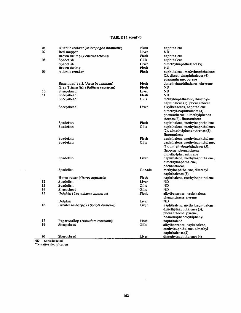
TABLE 15 . (conYd)

06 Atlantic croaker (Micropogon undulatus) 07 Red snapper

Brown shrimp (Penaeus aztecus) 08 Spadefish

Spadefish Brown shrimp

09 Atlantic croaker

Baughman's ark (Arca baughmani) Gray Triggerfish (Ballistes capriscus)

10 Sheepshead il Sheepshead

Sheepshead

Sheepshead

Spadefish Spadefish

Spadefish Spadefish

Spadefish

Flesh Liver Flesh Gills Liver Flesh Flesh

Flesh Flesh Liver Flesh Gills

Liver

Flesh Gills

Flesh Gills

naphthalene ND naphthalene naphthalene dimethylnaphthalenes (5) ND naphthalene, methylnaphthalenes (2), dimethylnaphthalenes (4), phenanthrene,pyrene dimethylnaphthalenes, chrysene ND ND ND methylnaphthalene, dimethyl- naphthalene (5), phenanthrene alkylbenzenes, naphthalene, dimethyl-naphthalenes (4), phenanthrene, dimethylphenan-threnes (3), fluoranthene naphthalene, methylnaphthalene naphthalene, methylnaphthalenes (2), dimethylphenanthrenes (3), fiuoranthene naphthalene, methylnaphthalene naphthalene, methylnaphthalenes (2), dimethylnaphthalenes (5), fluorene, phenanthrene, dimethylphenanthrene naphthalene, methylnaphthalene, dimethylnaphthalene, phenanthrene methylnaphthalene, dimethyl-naphthalenes (5) naphthalene, methylnaphthalene ND ND ND alkylbenzenes, naphthalene, phenanthrene,pyrene ND

Liver

Spadefish Gonads

Horse oyster (Ostrea equestris) Flesh 12 Spadefish Liver 13 Spadefish Gills 14 Sheepshead Gills 15 Dolphin (Coryphaena hippurus) Flesh

Dolphin Liver 16 Greater amberjack (Seriola dumerili) Liver naphthalene, methylnaphthalene,

dimethylnaphthalenes (3), phenanthrene,pyrene, "2-monophenoxybiphenyl

17 Paper scallop (Amusium texasiana) Flesh naphthalene 19 Sheepshead Gills alkylbenzenes, naphthalene,

methylnaphthalene, dimethyl- naphthalenes (2)

20 Sheenshead Liver dimethvlnanhthalenes (4) ND - none detected 'Tentative identification

162

obtained by GC. However, some additional o-alkanes were found in the samples due to the increased sensitiv-ity of the GC/MS method . The presence of phytane was confirmed in four instances . The most frequently con-firmed compounds in the unsaturated fraction were

naphthalene (20 times), squalene (19 times), methyl-naphthalene (14 times), dimethylnaphthalene (14 times), and phenanthrene (12 times) . A number of samples showed a suite of isomers for the alkyl benzenes and di-methylnaphthalenes similar to that observed in crude oil (Fig . 12) .

FIG. 12 . Extracted ion current profile of mass 141 (base peak of dimethylnaphthalene)-spadefish gills (upper) and empire crude oil (lower).

163

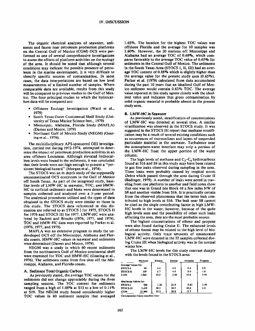
IV. DISCUSSION

The organic chemical analyses of seawater, sedi-ments and fauna near petroleum production platforms on the Central Gulf of Mexico (CGM) OCS were per-formed as one of several comprehensive investigations to assess the effects of platform activities on the ecology of the area . It should be noted that although several conditions may indicate the possible presence of petro-leum in the marine environment, it is very difficult to identify specific sources of contamination . In most cases, the data interpretations are based on low level measurements of a limited number of samples . Where comparable data are available, results from this study will be compared to previous studies in the Gulf of Mex-ico . The four principal studies to which the hydrocar-bon data will be compared are :

" Offshore Ecology Investigation (Ward et al ., 1979)

" South Texas Outer Continental Shelf Study (Uni-versity of Texas Marine Science Inst ., 1979)

" Mississippi, Alabama, Florida Study (MAFLA) (Dames and Moore, 1979)

" Northeast Gulf of Mexico Study (NEGM) (Gear-ing et al ., 1976) .

The multidisciplinary API-sponsored OEI investiga-tion, carried out during 1972-1974, attempted to deter-mine the impact of petroleum production activities in an area offshore Louisiana . Although elevated hydrocar-bon levels were found in the sediments, it was concluded that their levels were not high enough to present a "per-sistent biological hazard" (Morgan et al ., 1974) .

The STOCS was an in depth study of the supposedly uncontaminated OCS ecosystem in the Gulf of Mexico off South Texas . As part of the integrated study, base-line levels of LMW-HC in seawater, TOC, and HMW-HC in surficial sediments and biota were determined in samples collected and analyzed over a 3-year period . The analytical procedures utilized and the types of data obtained in the STOCS study were similar to those in this study . The STOCS data referenced in this dis-cussion are referred to as STOCS I for 1975, STOCS II for 1976 and STOCS III for 1977 . LMW-HC were ana-lyzed by Sackett and Brooks (1976, 1977, and 1979) . TOC and HMW-HC data were reported by Parker et al . (1976, 1977, and 1979) . MAFLA was an extensive program to study the un-

developed OCS off the Mississippi, Alabama and Flor-ida coasts . HMW-HC values in seawater and sediments were determined (Dames and Moore, 1979) . NEGM was a study in which 60 recent sediments

from the northeastern Gulf of Mexico continental shelf were examined for TOC and HMW-HC (Gearing et al ., 1976) . The sediments came from five sites off the Mis-sissippi, Alabama, and Florida coasts .

A. Sediment Total Organic Carbon As previously stated, the average TOC values for the

sediments did not change appreciably during the three sampling seasons . The TOC content for sediments ranged from a high of 1 .08% at S13 to a low of 0.11% at 519 . The NEGM study found considerably higher TOC values in 60 sediment samples that averaged

1 .65% . The location for the highest TOC values was offshore Florida and the average for 10 samples was 3.60%. However, the 20 stations off Mississippi and Alabama had an average TOC of 0.68%, which com-pares favorably to the average TOC value of 0.65% for sediments in the Central Gulf of Mexico . The sediments in the South Texas ,Area (STOCS I, II, III) had an aver-age TOC content of 0.88% which is slightly higher than the average value for the present study area (0.65%) . Parker et al . (1979) calculated from data accumulated during the past 10 ,years that an idealized Gulf of Mex-ico sediment would contain 0.63% TOC. The average value reported in this study agrees closely with the ideal-ized value and indicates that gross contamination by solid organic material is probably absent in the present study area .

B. LMW-HC in Seawater As previously noted, stratification of concentrations

of LMW-HC was detected at several sites . A similar stratification was observed in the STOCS study . It was suggested in the STOCS III report that methane stratifi-cation may be a result of several existing conditions such as occurrences of thermoclines and layers of suspended particulate material in the seawater. Turbulence near the atmosphere-water interface may strip a portion of the LMW-HC from the upper portion of the water column .

The high levels of methane and C2 -C4 hydrocarbons found at S16 and S8 in this study may have been related to gas line leaks observed during sampling in the area . These leaks were probably caused by tropical storm Debra which passed through the area during Cruise II (Bedinger, 1979) . A number of leaks were noted in trav-eling from one platform to another and field notes show that one was in Grand Isle Block 48 a few miles NW of S8 and another visible from 516 . It is practically certain from the observed phenomena that the latter leak con-tributed to high levels at S16 . The leak near S8 cannot be cited as the single contributing factor in high LMW-HC levels in the water ; however, because of the quite high levels seen and the possibility of other such leaks affecting the area, they are the most probable source .

The highest concentrations of ethene and propene were also found during Cruise II . The enhanced levels of ethene found may be related to the high level of bio-logical activity . Only trace amounts of unsaturated LMW-HC were detected in the 22 samples collected dur-ing Cruise III when biological activity was in the normal winter low .

The LMW-HC levels for this study contrast sharply with the levels found in the STOCS area :

Methane Ethane Ethene Propane Propene

Average Values for : STOCS-1 99 0.4 4.6 0.4 0.9 STOCS-11 339 1 .7 4 .8 0.9 1 .0 CGM 1,860 50 .9 2 .66 10.8 0 .49

Maximum Values for: STOCS-1 500 1 .30 25 .0 0.83 2.49 STOCS-111 5,410 58 .5 20 .5 16.6 2 .8 CGM 23,900 25 .2 38 .8 13 .7

Concentration Units nanoliter/ liter

165

Methane and CZ C4 saturated hydrocarbons were significantly higher in the present study area than those found in the STOCS area . The average levels of ethene and propene were slightly higher in the STOCS area .

In a study by Swinnerton and Lamontagne (1974), baseline measurements of LM W-HC were determined in open ocean and near shore water samples . A contami-nation index (CI) based on the average concentrations of methane, ethane, and propane was proposed to dif-ferentiate between open ocean, clean water and water contaminated by hydrocarbons :

CI =1/3(C,/C, + CZ/CZ + C3/C3)

where C,*, CZ and C3 are the averages of open ocean concentrations of methane, ethane and propane, re-spectively . Average values used in the calculation of CI were 49.5 nl/1 for methane, 0.50 nl/1 for ethane, and 0.34 nl/1 for propane . Based on concentrations in the open ocean, a CI greater than 5 indicates hydrocarbon contamination .

It was found that most sites in the present study area had abnormally high CI values indicating that methane, ethane and propane levels were considerably above open sea levels . The average CI level found for the control sites was 30.8 . Therefore, it was felt that the standard CI determination may not be useful when applied to the present study area since the entire baseline level for the area was much higher than open sea levels . The high lev-els over the entire study area, which encompasses seve-ral major gas production areas, may be a result of production-related activity such as brine discharge, un-derwater flaring and gas line leaks . Other contributions from natural sources may include natural gas seepages from subsurface faults and shallow biogenic gas from organic rich sediments . Other possible hydrocarbon sources which have not been investigated, such as Mis-sissippi River waters and leakage from tanker lightening operations conducted in the delta area, may contribute to the high levels of LMW-HC found in the CGM study area .

To locate areas of unusually high levels of LMW-HC, it was necessary to compare primary and secondary platforms to the control sites in order to determine the baseline values for the area . Since the average concen-trations of LMW-HC fluctuated during the three cruises, it was necessary to compare each platform for each cruise to the control sites for that particular cruise . The seasonal variations in the average concentrations of LMW-HC at the control sites was probably a result of wave intensity, current changes and water temperature . A comparative index for LMW-HC (LCI) patterned after the CI equation was derived as follows :

LCI = 1/2 [(C1/Cl-) + (CZ + C3 + iC4 + nC4)/(CZ + C3 + iC: + nC4 )]

where C,* is the average methane concentration for the control sites for each cruise (1560, 2260, and 646 nl/1 for Cruises I, II and III, respectively), and (CZ + C3 + iC4 + nC4 ) is the total average concentration of ethane, propane, isobutane and n-butane for the control sites for each cruise (47 .2, 44.8 and 0.93 nl/1 for Cruise I, II and III, respectively) . The values used for C, and (CZ + C3 + iC4 + nC4) were the average concentrations for each site . LMW-HC and LCI values are tabulated in Appendix B2.

Swinnerton and Lamontagne (1974) determined the criterion Contamination Index for their data by examin-ing the CI values for samples which they collected in the open sea . Their highest CI values in open seawater were near three . Therefore, samples collected near shore in their study which had CI values greater than three but not greater than five were classified as possibly contami-nated . Samples which had CI values greater than five were considered contaminated . The LCI values for the control sites in the present study were much closer in distribution . The highest LCI value for a control site was 1 .71 at C23 in Cruise I . Therefore, LCI values above 3.0 are considered significantly above the baseline level for the study area since these values are at least three times higher than the average control site value and nearly twice as high as the highest value found at the control sites .

The LCI values for Cruise I samples were 1 .75 or less (Fig . 13) . For Cruise II, three sites were found to have values significantly above the baseline level (Fig . 14) . These were S8, S16, and S18 with LCI levels of 8.94, 3.58, and 12.2, respectively (Fig . 14) . The probable rea-son for these high values at S8 and S16 was the previ-ously discussed gas line leaks . The production platform at S18 discharges daily 12-15 thousand barrels of brine, which may be introducing LMW-HC into the local area . All other sites sampled during Cruise II had LCIs equal to or less than 1 .52

Samples taken during Cruise III were generally much lower in LMW-HC content, as exemplified by the low average values for Cruise III control sites, except for Sites P2 and P4 which had LCI values equal to 4.30 and 115, respectively (Fig. 15) . Platform 2 is discharging a large amount of brine and Platform P4 is venting excess gas underwater, both of which may be contributing to the LMW-HC levels . Therefore, it is likely that these platform-related activities are elevating the amount of LMW-HC in the seawater in the vicinity of these plat-forms . During the first two cruises, high values of LMW-HC were not detected at these platforms perhaps because samples were taken at only 100 m north of the platform and possibly the currents fluctuated suffi-ciently for the sampling during Cruises I and II to be up-stream from the platform .

C. HMW-HC in Sediments

1. Total Hydrocarbons Concentrations of total hydrocarbons extracted

from surficial sediments ranged from a high (average for platform) of 87.2 lAg/g at S6 to a low of 5.7 Ng/g at S19 with an average of 36.5 1Ag/g (Appendix B.3 .) . The HMW-HC in surficial sediments from the control sites were compared with those from the primary and sec-ondary platforms by a comparative index (HCI) which was derived as follows :

HCI = (HMW-HC)/(HMW-HC*)

where HMW-HC is the average measured HMW-HC (ug/g) found in sediments at a platform site and HMW-HC* is the average measured HMW-HC found in sediments at control sites . Average HMW-HC con-tent found at each primary platform during the three sampling seasons was compared to the average HMW-HC content found in control site samples during those

166

v

V ~ FRANKLIN

BARATARI" v V

\\V

WEN CUM 41A10E ~. MOR(iAN CITY

v ~w N

~

1\

v YARfM 1. I '~

NOUMA �, ' e e

-0

~rC L 1 c t

1

~ - ~^~ L ~ v

vy~

r - c~ GOLDEN

~ MEADOW

K wQ ~~!! ,,,,~~

AU FIR 1 . ZS ~) ~J VENICE

GRAND ZI I ISLE

Cv( ~ TERIIEIONIIE II; � - - '- r yy

° ~~o~`~ ; . ~ " 2

022

1

. - " 3 --- - ., -- . . -- --- t - - ------- . . SCALE 04

DIAMETER OF CIRCLE

23 - 0.0

- 3.0

" . SCALE , .

--------- ,_ . -----------------------

""'"- ------

---- --- __ . . ----

--- 1"qU5M105 Of PETERS

FIG. 13 . LCI values for Cruise I. (The zipatone pattern indicates sites where LMW-HC were significantly above control site levels).

,S FRANKLIN

a 00

10tlT COR

__ 4r

IYMIiN 1 .

MORGAN CITY

NOUIIA i f

4re

fttiy~ i

rr w ro~i

18 .-

`0 24

14

0

is

023

017 19

-04 - SCALE DIAMETER OF CIRCLE

- 0.0

by - 3.0

SCALE ~ o i z

7"OUSANDS OF METERS

* BARATARIA

1p4

" '"

GOLDEN MEADOW

f 21 enISLE~wo ~

~ A - - --

Y CV~~ iE1ME~ONNE "AY ~ I

PJ ~Not

~ 13~ 0 19

1320 _10

-022 49

m ~ " 7 . ,_ .

09

---- -------

FIG. 14 . LCI values for Cruise II . (The zipatone pattern indicates sites where LMW-HC were significantly above control site levels) .

a

V ,` FRANKLIN

BANAIARIA \V1

WEST COR KA"M 110RGAN CITY f

a DAY

1 v tf

emu, ~, 11

YAIqN 1 . '~ HdJYA w

''

C ~

,rch _

l 2

C r k, 4 V i 14

r c - ~ GOLDEN MEADOW

PT ~u rpi i . - U VENICE

"

`

GRAND 21

C4,4 TERnEmONNE "Y

` d p 2

. . I 022

L` 3 -- - -------- ---- --- t '

., -- - -- -- ------- 4 ,_ SCALE

DIAMETER OF CIRCLE

a - 0.0 23

: . - 3.0

SCALE ., , . . . _,

. . -- '-" TNOVSANDS OF METERS

FIG. 15 . LCI values for Cruise III. (The zipatone pattern indicates sites where LMW-HC were significantly above control site levels) .

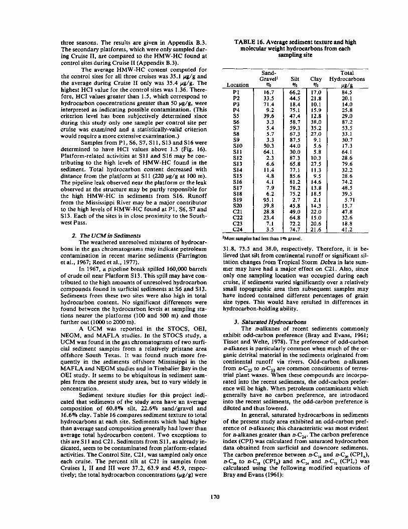
three seasons. The results are given in Appendix B.3 . The secondary platforms, which were only sampled dur-ing Cruise II, are compared to the HMW-HC found at control sites during Cruise II (Appendix B.3) .

The average HMW-HC content computed for the control sites for all three cruises was 35.1 Mg/g and the average during Cruise II only was 35.4 Ng/g . The highest HCI value for the control sites was 1 .36 . There-fore, HCI values greater than 1.5, which correspond to hydrocarbon concentrations greater than 50 1Ag/g, were interpreted as indicating possible contamination . (This criterion level has been subjectively determined since during this study only one sample per control site per cruise was examined and a statistically-valid criterion would require a more extensive examination .)

Samples from P1, S6, S7, S11, S13 and S16 were determined to have HCI values above 1 .5 (Fig . 16) . Platform -related activities at Sil and S16 may be con-tributing to the high levels of HMW-HC found in the sediment . Total hydrocarbon content decreased with distance from the platform at S11 (220 jug/g at 100 m). The pipeline leak observed near the platform or the leak observed at the structure may be partly responsible for the high HMW-HC in sediments from S16 . Runoff from the Mississippi River may be a major contributor to the high levels of HMW-HC found at P1, S6, S7 and 513 . Each of the sites is in close proximity to the South-west Pass .

2. The UCM in Sediments The weathered unresolved mixtures of hydrocar-

bons in the gas chromatograms may indicate petroleum contamination in recent marine sediments (Farrington et al ., 1967 ; Reed et al ., 1977) .

In 1967, a pipeline break spilled 160,000 barrels of crude oil near Platform 513 . This spill may have con-tributed to the high amounts of unresolved hydrocarbon compounds found in surficial sediments at S6 and 513 . Sediments from these two sites were also high in total hydrocarbon content . No significant differences were found between the hydrocarbon levels at sampling sta-tions nearer the platforms (100 and 500 m) and those further out (1000 to 2000 m).

A UCM was reported in the STOCS, OEI, NEGM, and MAFLA studies . In the STOCS study, a UCM was found in the gas chromatograms of two surfi-cial sediment samples from a relatively pristane area offshore South Texas. It was found much more fre-quently in the sediments offshore Mississippi in the MAFLA and NEGM studies and in Timbalier Bay in the OEI study . It seems to be ubiquitous in sediment sam-ples from the present study area, but to vary widely in concentration .

Sediment texture studies for this project indi-cated that sediments of the study area have an average composition of 60.8% silt, 22.6% sand/gravel and 16.6% clay . Table 16 compares sediment texture to total hydrocarbons at each site . Sediments which had higher than average sand composition generally had lower than average total hydrocarbon content . Two exceptions to this are S11 and C21 . Sediments from 511, as already in-dicated, seem to be contaminated from platform-related activities . The Control Site, C21, was sampled only once each cruise . The percent silt at C21 in samples from Cruises I, II and III were 37.2, 63 .9 and 45.9, respec-tively ; the total hydrocarbon concentrations (fig/g) were

TABLE 16 . Average sediment texture and high molecular weight hydrocarbons from each

sampling site

Sand- Total Gravel' Silt Clay Hydrocarbons

Location % % % / P1 16.7 66.2 17 .0 84.5 P2 33.5 44.5 21 .8 20.1 P3 71 .4 18 .4 10 .1 14.0 P4 9.2 75.1 15 .9 25 .8 S5 39.6 47.4 12.8 29.0 S6 3.3 58.7 38.0 87.2 S7 5.4 59.3 35 .2 53 .5 S8 5.7 67.3 27.0 33 .1 S9 3.3 87.5 9 .1 30 .7 S10 50.3 44.0 5 .6 17 .3 S11 64 .1 30.0 5 .8 64.1 S12 2.3 87.3 10 .3 28 .6 S13 6.6 65.8 27.5 79.6 S14 11 .4 77.1 11 .3 32.2 S15 4.8 85.6 9 .5 28.6 S16 4 .1 81 .2 14.6 74.2 S17 7.9 78.2 13 .8 48.5 S18 6.2 75.2 18.5 39.5 S19 95 .1 2 .7 2 .1 5 .71 S20 39.8 45.8 143 15 .7 C21 28.8 49.0 22.0 47.8 C22 23 .4 64.8 15 .0 32.6 C23 7.1 72.2 20.6 18 .8 C24 3 .5 74.7 21 .6 41 .2

Most samples had less than 1 % gravel

31 .8, 73 .5 and 38.0, respectively. Therefore, it is be-lieved that silt from continental runoff or significant sil-tation changes from Tropical Storm Debra in late sum-mer may have had a major effect on C21 . Also, since only one sampling location was occupied during each cruise, if sediments varied significantly over a relatively small topographic area then subsequent samples may 'have indeed contained different percentages of grain size types . This would have resulted in differences in hydrocarbon-holding ability.

3. Saturated Hydrocarbons The n-alkanes of recent sediments commonly

exhibit odd-carbon preference (Bray and Evans, 1961 ; Tissot and Welte, 1978) . The preference of odd-carbon n-alkanes is particularly common when much of the or-ganic detrital material in the sediments originated from continental runoff via rivers . Odd-carbon n-alkanes from n-Cys to n-C33 are common constituents of terres-trial plant waxes . When these compounds are incorpo-rated into the recent sediments, the odd-carbon prefer-ence will be high . When petroleum contaminants which generally have no carbon preference, are introduced into the recent sediments, the odd-carbon preference is diluted and thus lowered .

In general, saturated hydrocarbons in sediments of the present study area exhibited an odd-carbon pref-erence of n-alkanes ; this characteristic was most evident for n-alkanes greater than n-C2, . The carbon preference index (CPI) was calculated from saturated hydrocarbon data obtained from surficial and downcore sediments . The carbon preference between n-C� and n-Cm (CPI), n-C, to n-C, (CPI,) and n-C, and n-C,, (CPI) was calculated using the following modified equations of Bray and Evans (1961) :

170

v ~ FRANKLIN V~v

P BARATARIA \~V

WEST COTf BLANCHE MORWN CITY fv u

MOUIAA YMlM 1 . k~ ~

(~-~~ S( i j

PC 44P ~.J C ?

i ~ s 14~ a

GOLDEN ~J MEADOW

PL Z,w iG )S 9J "u fER i .

VENICE

" GRAND 2 ISLE ' S

.,r

I. 12 Allk

8 '--

13 I W22

Is 019 20

. . - .1Q~

14 _ 3 9 .

~ -- - . . t -----------------------

q - SCALE is DIAMETER OF CIRCLE

023 - 0.0

> :2 - 1 . 5

AdIlk IT .. . .....

15 4 2 3 4 _ . . . . . . . . . .

~2 Y ---------------------------------

TNOUSYID3 0F YETERS - "; "O . _

FIG. 16. High molecular weight hydrocarbon comparative index values for all stations .

CPI, = 1/2 [(Cis + Cp +Ci9)ACIa + Cis + Cps) + (C" + C, + C,9)/C,6 + C18 + C20)]

CPI, = 1/2 [(CZ, + C23 + CZS + C27)/(C20 + CZZ + Cu + Cam) + (CZi + CZ3 + CZS + C27)/(C22 + Cu

+ CZ6 + Cam)]

CPI 1/2 [(C21 + CZ7 + CZ9 + C;,)/(C2, + C26 + C28 + Cam) + (CZS + CZ7 + C29 + C3,)/(C26 + C,

+ C30 + C32)]

Averages for values of CPI,,,, and c for each site are given in Table 17 . For all sites and all cruises, the average CPIA was 1 .11 ; the average CPIB was 3.12 ; and the average CPI was 6.37 . Six sites with the highest CPI values were P1, P3, S7, S13, S17 and C21 .

TABLE 17 . CPI for saturated hydrocarbons extracted from surficial sediments

CPIA CPIB CPI (n-C,4 to (n-C20 to (n-C24 to

Site o-C20) n-C28) o-C3Z)

P 1 1 .46 4.21 8 .42 P2 1.12 2.93 6.22 P3 1 .27 2.98 8.31 P4 1 .37 3 .19 6.97 S5 1 .37 3 .86 5.66 S6 1 .18 3 .20 5.55 S7 1 .25 2.72 7.74 S8 0.76 2.92 6.92 S9 1 .05 2.87 4.50 S10 1 .03 2.30 4.27 S11 1 .06 3 .18 4.21 S12 1 .31 3 .09 6.57 S13 1 .15 3 .36 8.25 S14 0.73 2.72 4.86 S15 0.88 2.24 5.19 S16 1 .07 2.81 4.42 S17 0.66 3 .02 7.67 S18 1 .21 3 .03 5.28 S19 1 .29 2 .01 2.90 S20 1 .31 2.97 6.65 C21 0.82 3.62 8.85 C22 1 .15 2.63 5 .11 C23 0.94 3 .03 5 .09 C24 0.92 3.58 5 .71

Sediments from S11 had an average CPIA of 1 .06 . The saturated hydrocarbons from this platform contained large concentrations of C,3, C,4 and C,5 n-alkanes with C13 and C14 being dominant peaks . They may be petroleum hydrocarbon contaminants .

Platform S19 had some of the lowest CPI val-ues . Also sediments from this platform had the least amount of total hydrocarbons (5.71 Mg/g) ; however, this is probably a consequence of the sandy nature of S19 sediments (see Table 16) .

The average ratio of pristane to phytane for all cruises was 1 .15 ; pristane to n-C, 7, 1 .09 ; and phytane to n-C,8, 0.67 . These values are less than those found at two sites off Mississippi in the NEGM study (1 .73, 2.31, 2.80, respectively) .

The average CPIA, CPIB and CPI values in the downcore samples were 0.97, 2.24, and 4.65, respec-tively. These values are less than those found in the sur-ficial sediments and in the case of CPI would suggest

that the downcore samples were more contaminated by petroleum hydrocarbons than were the surficial sediments.

4. Unsaturated Hydrocarbons Unsaturated hydrocarbons were found at all

platform sites . Typical unsaturated hydrocarbon GC patterns indicated an extensive mixture of aromatic and polyunsaturated hydrocarbons which often resulted in an unresolved envelope . GC and GC/MS analyses indi-cated the presence of compounds typified as pyrogenic and petrogenic aromatic hydrocarbons as well as some anthropogenic compounds at many sites . This indicates that many sites are experiencing contamination by un-saturated hydrocarbons from multiple sources .

Anthropogenic compounds (phenoxybiphenyls and/or polychlorinated biphenyls) searched for by GC/MS, were detected in sediments at P1, S5, S16, S17 and S18 . Platforms P1 and S5, which are relatively close to both the coastline and the Southwest Pass, contained these compounds, but they were not detected at a nearby Control Site (C21) . Platforms 516, S17 and S18 are the sites which are farthest from the mouth of the Mississippi River and they contained this class of compounds.

Pyrogenic compounds such as pyrene, fluoran-thene and benzo(a)pyrene were detected at all sampling sites .

The key petrogenic aromatic hydrocarbons are the alkyl aromatic hydrocarbons and their isomers . Spe-cific alkyl aromatic hydrocarbons which were mon-itored in this study were methylnaphthalene, dimethyl-naphthalene and dimethylphenanthrene . Each site, in-cluding the control sites, contained alkyl aromatic hydrocarbons . Platforms which contained multiple isomers of these compounds (a very strong indication of petroleum contamination) were P1, P2, P3, S7, S8, 512, S15 and 517 . The presence of isomers was determined by GC/MS. Of the six sites which contained high HCI values, three were checked by GC/MS (P1, S7 and S16) . Platforms P1 and S7 contained relatively high concen-trations of the isomers while no isomers were detected in the sample from 516 .

D. Hydrocarbons in Fauna The results suggest that a significant number of or-

ganisms in the study area have been exposed to low lev-els of petroleum and pyrogenic hydrocarbons. The pet-rogenic nature of a portion of these hydrocarbons is in-dicated by the presence of the alkyl derivatives of 1, 2, and 3-ring aromatics . For example, GC/MS'analysis of Empire crude oil showed that the ratio of CZ alkyl homologues of 3-ring aromatics to the parent com-pounds was 1 .4 . However, differences in solubility and possible metabolic changes make it difficult to predict what this ratio would be in a given tissue if the com-pounds originated only from petroleum .

The problem is further complicated by the presence of combustion products (e.g ., benzopyrene, pyrene, and fluoranthene) . Their presence in pristane sediments has been attributed to atmospheric fallout of products re-sulting from fossil fuel usage (Hites, LaFlamme, and Farrington, 1977 ; Brown and Starves, 1978) . However, that these compounds were rarely found in tissues in the STOCS or MAFLA programs and that they were in tis-sues from the present study area indicates that levels of these materials are elevated in the study area .

172

All that can be concluded is that the organisms in the study area are probably being exposed to both petro-genic and combustion-related hydrocarbons . Qualita-tive assessment of the data suggests that the relative sig-nificance of either process may be related to location ; e.g ., the contaminated organisms obtained from Plat-form S11 (Table 15) contained alkyl homologues as well as parent compounds, whereas the aromatic profile of organisms at SS is dominated by the parent compounds (biphenyl, phenanthrene, pyrene, fluoranthene, and benzopyrene) .

It is interesting that the compound tentatively identi-fied as a phenoxybiphenyl (=1 ppm) found in the greater amberjack (Seriola dumerih) at Platform S16 was also found in high levels in the sediments nearby . With the exception of this compound, all of the GC/MS con-firmed aromatics were in the 1-70 ppb range .

The conclusions reached by recent studies both in the Gulf of Mexico and elsewhere have generally fallen into two groups-those that demonstrate little or no evi-dence of petroleum contamination of tissues (STOCS ; MAFLA; Shaw and Baker, 1978) and those that show significant levels of petroleum hydrocarbons and/or pyrogenic aromatics (Dunn and Stich, 1975 ; Bravo et al ., 1978 ; Middleditch and West, 1979) . This may reflect the emphasis in previous studies of this type and the ini-tial design of this study, i .e ., to monitor primarily the n-alkanes and the higher aromatics (3 rings or more) . This approach is not ideal for determining low level ex-posure to petroleum .

Study of the saturated hydrocarbon fraction (pris-tane/phytane and CPI ratios) will probably not reveal low level contamination for the following reasons :

Although the n-alkanes are a major component of crude oil, they disappear with time due to weathering . The solubility of n-alkanes prevents them from being as readily accessible to organisms as other, more polar constituents of petroleum . The presence of biogenic alkanes may mask low levels of petrogenic alkanes .

Similarly, searching for 4- and 5-ring aromatics in tissues will not be useful for detecting low levels of pe-troleum contamination inasmuch as these compounds exist in very low concentrations in crude oil and are rela-tively insoluble in water . Unresolved envelopes, al-though valuable for the study of sediments and highly contaminated tissues, are of no use in detecting low level tissue contamination .

Low level input of petroleum hydrocarbons may be better indicated by searching for benzene and naphtha-lene and their alkyl-substituted isomers . The solubility of these compounds and hence their availability to ma-rine organisms is significantly greater than other hydro-carbon components of petroleum . In the future, meth-ods of screening for petroleum contamination should be modified so that the more volatile aromatics are de-tected reliably. Perhaps either purge and trap and head-space techniques together with selective aromatic GC detection (e .g ., photoionization) could be used for such analyses .

E. Synthesis of Results The purpose of the data synthesis on the organic

chemical data was as follows :

To correlate concentrations of hydrocarbons in sediments and benthic and pelagic macrofauna with proximity to and age of platforms studied, with emphasis on potentially toxic compounds; To correlate concentrations of hydrocarbons in downcore sediments of various ages with proxim-ity to and the age of platforms studied, with esti-mated age of the sediments analyzed, and with initiation of petroleum exploration, development, and production in the overall study area ; To determine the probable or possible impact of known spills, discharges, or other sources of petroleum-activity-related contaminants on the study area in general and on the samples collected and analyzed ; to review other known sources of pollutants in the study area ; and to discuss the Mississippi and Atchafalaya Rivers' discharges in terms of magnitude and contaminant loading, and potential impact on the study area ; To discuss the effects of human consumption of seafood products containing various levels of hy-drocarbon compounds including contaminant levels and seafood consumption necessary to pro-duce a probable effect .

The results of these synthesis tasks are discussed below.

l . Correlation of Hydrocarbon Contamination with Platform Characteristics From the data obtained on the analyses of sedi-

ments and biota for hydrocarbon content, the following platforms were judged to show some indication of envi-ronmental pollution arising from platform-related activities :

Sediments-Pl, S6, S7, S11, S13, S16 Biota-P4, S9, S11, 516, 519, S20

These designations are made on the basis of the HCI as described for the sediments and on the presence of aro-matic compounds in the benthic and pelagic macro-fauna as confirmed by GC/MS. These results are dis-cussed in previous sections .

To supplement these investigations, the levels of total hydrocarbons in the sediments were evaluated to see if there was a trend toward decreasing concentra-tions with distance from the platform . The platforms where this trend was observed included : P1 (Fig . 17), S6, S7, 510, S11, 512, 513, 514, 516, and S17 (Table 18) . The total hydrocarbons in the sediment were used since this includes the UCMs of both saturated and un-saturated fractions . The UCMs characteristically con-tained upwards of '75% of the total fraction and are gen-erally considered to be representative of pollution rather than natural input . . Examples of the trends observed are shown in Fig . 18, which gives examples of a trend and no trend for each of the primary and secondary plat-forms, respectively . This trend was most evident at 511, where the 100-m station had a concentration of total hy-drocarbons in excess of 200 jAg/g, and the remaining sta-tions had concentrations of less than 15 1Ag/g . Platforms S6, S13, and S16 showed values in excess of 100 lAg/g at the 100-m station with lower values at the farther dis-tances, and P1 had a range of 96 to 370 pg/g for the four 100-m stations in Cruise I . At the other platforms cited above, the concentration at the closest station was

173

NORTH

63.0 2000 m

39.7 1000 m

15.3 500 m

189.5 100 m

J A

T_4 WEST 60.4 14.6 22.5 96.4 PLATFORM 159.3 36.7 102.6 40.8 EAST

3

0 100 M

2000 m 1000 m 500 m 100 m 100 m 500 m 1000 m 2000 rn 70.7 100 M

28.5 [ 500 m

46.9 1000 m

38.9 2000 m

SOUTH

FIG. 17 . The total hydrocarbon concentration (fig/g) in the sediments near P1 (Cruise I) . This shows a trend toward decreasing concentration with distance from the platform .

v U

N

63 2000 m

40 1000 m

15 500 m

189 100 m

60 ~5 22 9~ PLATFORM 1~ 37 103 41 6 8 27 5

2000 m 1000 m 500 m 100 m 100 m 500 m 1000 m 2000 m 2000 m 1000 m 500 m 100 m

371 100 m

yg 500 m

47 1000 m

39 ~ m

P7 SECONDARY SITES

Z4

7

23

223

U 38

S71 S15

2 2000 m

14 1000 m

g 500 m

7 100 m

PLATFORM 32 6 13 7

100 m 500 m 1000 m 2000 m

63 100 m

9 500 m

24 1000 m

37 2000 m

P2

FIG. 18 . Typical sediment hydrocarbon gradient patterns at primary and secondary platforms. Values given are for total hydrocarbons, jAg/g dry weight .

TABLE 18 . Total hydrocarbon concentration (fig/g) at secondary platforms with increasing distance from

the platform

Platform loom, 500 m 1000 m 2000 m S5 25 .5 41 .1 42.0 7.6 S6 84.8 131 .0 49.1 43.5 S7 67.8 47.4 60.2 38 .5 S8 34.0 21 .5 54.0 22.8 S9 13.2 19.5 39.4 50.4 S10 32.2 4 .0 8 .6 24 .1 SI1 222.7 11 .6 7 .3 13 .9 S12 43.6 18 .8 36.8 15 .1 S13 105 .1 75 .6 87 .3 54.4 S14 64.5 37 .2 19.0 8.2 S15 38 .2 23 .0 30.0 23 .6 S16 106.7 84.9 55 .1 49.7 S17 76.4 61 .6 29.5 13.6 S18 41 .6 75 .9 10.0 30.6 S19 3 .4 8.3 5 .5 5 .7 S20 35 .0 7.6 15.4 4.7

All sampling was north of the platform .

not considered unusually high for the study area (gener-ally 40 to 70 Ng/g), but an apparent gradient existed with distance . This decreasing concentration with dis-tance may imply that the platforms and/or their related activities are the source of elevated levels of hydrocar-bons in the surrounding environment . This fact, when coupled with the results of the LMW-HC and biota analyses, leads to an ordering of platforms on the basis of level of indicated platform-related effects. This is as follows :

High : P1, S7, 511, S16 Medium : P4, SS, S8, S9, 515, 517, S18, 519, S20 Low: P2, P3, S6, S10, S12, 513, S14

This classification was based on the following scheme . The factors given highest priority were the pres-ence of high hydrocarbon levels in the sediments, the presence of a gradient of decreasing sediment hydrocar-bon concentrations away from the platform, and the confirmation of petrogenic chemicals in the biota . The seawater hydrocarbon data were given lower priority .

The only sites which had aromatic hydrocarbons in both the sediments and the biota were Platforms S11 and S16, which were placed in the high effects category along with Platform P1 and Platform S7 . Although Platform P1 is located close to the mouth of the Missis-sippi River and has high hydrocarbon levels as a result, the presence of a gradient of decreasing concentration with distance from the platform implicated the platform as a source above and beyond the background levels . Platform S7 had both high levels of hydrocarbons in the sediment and a decreasing concentration gradient with increasing distance from the platform .

The medium effects group contains those plat-forms implicated by at least one of the studies . Plat-forms P4, S9, 519, and S20 were placed in the medium effects category on the basis of biota data . Platforms S5, S8, S15, S17 and S18 were placed in this group based on one or more of the following : LMW-HC, presence of petrogenic compounds in sediment, and low CPIA.

The low effects group consists of those plat-forms which give no real indication of platform-related pollution . This category includes S6 and S13 which, although cited for high sediment hydrocarbon values, exhibited only a slight trend toward decreasing concen-tration with distance . The values observed for these platforms could have resulted from river influence and therefore they were assigned to the low effects group .

An attempt was made to ascertain a relationship between the hydrocarbon concentration and the age of the platform, level of production, and type of produc-tion . These investigations are summarized below .

TABLE 19. Ages of study area platforms

Age in Years Platform (as of 1979)

P1 17 P2 25 P3 11 P4 15 SS 17 S6 14 S7 14 S8 22 S9 14 S10 24 S11 22 S12 17 S13 11 S14 6 S15 5 S16 8 S17 7 S18 9 S19 19 S20 10

The age of the platform is shown in Table 19 for each of the study platforms . The platforms were arbi-trarily divided into three age groupings : 5-8 years, 9-17 years, and 22-25 years . If there were no relationship between environmental levels of hydrocar-bons and age of the platform, then the distribution of platforms by age should be mirrored by the distribution of age at each of the exposure levels . Expected fre-quencies (EU) for this evaluation were calculated by the formula :

Eu = (R .) (C) N

where EU = expected frequency in the i row, j column of the array

R; = number of items in row i Ci = number of items in column j and N = total number of platforms

A contingency table of age versus exposure level is given below showing the observed number of plat-forms in each exposure and age group followed in par-entheses by the expected number of platforms for each group .

176

AGE/EXPOSURE DISTRIBUTION Exposure

A e rs High Medium Low Ri 5-8 1 2(2.25) 1(1 .75) 5 9-17 2 4(4.5) 4(3 .50) 10

22-25 1 2(2.25) 2(1 .75) 5 C~ 4 9 7 N=20

As can be seen, the expected frequencies match the observed frequencies very closely . A chi-square test for independence yields a value of

Xz = 0.54

with 4 degrees of freedom and is clearly not significant. The conclusion is that the environmental effect on the surrounding area is unrelated to the age of the platform .

Similar investigations were conducted for pro-duction level and type of production . Using the number of wells drilled from a particular platform as the indi-cator of level of activity, a contingency table was con-structed as shown below :

DRILLING LEVEL/EXPOSURE DISTRIBUTION Exposure

No. of Wells High Medium Low Ri 1-7 0(0.4) 2(0.7) (0.19) 2

12-18 4(2.6) 4(4.5) 5(5 .8) 13 21-24 0(1 .0) 1(1 .8) 4(2.3) 5 C: 4 7 9 N=20

The test for independence between these factors gives a chi-square value of 7.25, which is not significant . The conclusion is that the levels of hydrocarbons arising from the platform-related activities are not attributable to the number of wells drilled .

The cumulative production of oil in barrels and gas in Mcf were obtained for 17 of the 20 platforms studied . These were grouped into three frequency classes for oil and four for gas . Contingency tables are shown as follows :

PRODUCTION OF OIL/EXPOSURE DISTRIBUTION Exposure

Oil Production (bb1X10-6) High Medium Low Ri

18.4-27.9 1(1 .4) 2(2.S) 3(2.1) 6

za16.o uo .7)

]

1(1 .z) a1 .p 3 0.2- 2.6 1(1 .9) 4(3 .3) 3(2.8) 8 C 4 7 6 N-17

PRODUCTION OF GAS/EXPOSURE DISTRIBUTION Exposure

Gas Production (MotX10-6) High Medium Low Ri

138 .1-170 .3 1(0.5) 1(0.8) 0(0 .7) 2 21 .4- 57 .3 0(1 .4) 4(2 .5) 2c21 .0> e 9 .9- 18 .< 2(1 . .> 2(2 .5) 2(2 .1) 1.1- 5.4 1ro.1>> 0(1.2) 2(1 .1) 3

Ci 4 1 6 N-17

For neither oil nor gas production was there a significant relationship between production and relative

environmental contamination, with Xz values of 4.74 and 5.98, respectively .

The overall conclusion, then, is that a plat-form's being a source of hydrocarbons in the environ-ment cannot be correlated with the age or production-activity level of the platform .

2. Correlation of Hydrocarbons in Downcore Sedi-ments with Historical Development of the Study Area The investigation of hydrocarbons in downcore

sediments with respect to age of the platform and dis-tance from it could not be successfully completed . The dating of the cores, as previously discussed, revealed that either extensive mixing had occurred during the coring process and no accurate time frames could be es-tablished or that the sediments themselves are quite well mixed . The data also indicate that some additional phe-nomenon had taken place, either as a result of the sampling process or some activity in the ocean which is not understood at this time . For both the total hydro-carbons determined for the sample and the specific aro-matic hydrocarbons selected for study, the tendency was for the highest concentrations to be found in the deepest interval .

Two mechanisms which would result in the upper layers of sediment containing less total hydrocar-bons are (1) a continuous cleansing of the upper layer by dissolution and (2) a covering of the hydrocarbon-con-taminated layer by fresh uncontaminated sediment . The solubilities of many of the petroleum hydrocarbons in seawater are greater than 1 ppm as exemplified by naph-thalene, 1-methylnaphthalene and biphenyl which have solubilities of 31 .3, 25 .5 and 4.76 ppm, respectively (Eganhouse and Calder, 1976) . Given large volumes of seawater passing over the surface and possibly through a nepheloid layer, a . significant amount of hydrocarbons would be stripped from the upper few centimeters . If the hydrocarbon-contaminated sediment were covered by a fresh sediment layer, then the sediment would be protected from the dissolution process and the hydro-carbon's residence time in the sediment would be increased .

Attempts were made to resolve the presence of the concentrations by relating them to the grain size of the downcore sediments ; however, particle size analyses revealed no major differences with depth which might affect the concentrations observed . In addition, the particle size analysis of the top ten centimeters did not correspond to the analysis of the surficial sediments from the same sites . This raises the possibility that the surficial layer of the downcore sample was possibly lost or severely disturbed during the coring operation, which would also adversely affect the results of this investigation .

The only conclusion, then, is that there is an in-crease in sediment hydrocarbon contamination with depth in the sediment column for reasons presently unknown .

3. Impacts of Known Spills, Discharges and Other Sources of Petroleum-activity-related Contami-nants

a . Known :Spills Platforms S12 and S13 have been identified

and discussed in Part i as being near the sites of

177

previous oil spills . Platform S12 has been identified in this report as being a site which, based on total hydro-carbon determinations, appears to exhibit a gradient of decreasing contamination away from the structure . Since the spill in 1971 was some 600 m WSW of the plat-form and the four samples analyzed in this study were taken on a north transect it is not possible to conclu-sively determine whether the decrease in concentration was due to the platform or the spill . However, since lev-els of sediment HMW-HC are relatively low and in the range of nearby platforms and C22 (Fig . 16), it is sug-gested that the apparent platform source is likely and that the earlier spill has not caused a remaining residue higher than surrounding sites .

Platform S13 has been discussed as defini-tively contributing to contamination in fauna of the area, as confirmed by GC/MS demonstration of aro-matic compounds indicative of petroleum sources ; and it exhibits among the highest levels of HMW-HC in sed-iments, as shown by the HCI (Fig . 16) . This implicates the site as one which could have been affected by the nearby spill . The spill site was to the NW of the plat-form and sampling was to the N ; therefore, it is conceiv-able that any gradients from the spill or the platform might cancel out each other . No gradients away from the platform were found . Absolute levels of hydrocar-bons and total organics at this location were among the highest found, as were the levels of TOC at nearby S6, S7 and S9 (Fig . 7) and the HCI at P1, S6 and S7 (Fig. 16) . Thus, as has been previously discussed, it is quite possible that either total production from this highly de-veloped area or more probably the Mississippi River is providing the sediment contaminant load . This is not to say that the aromatics found in associated fauna are not from the platform .

Review of the OCS events file on the plat-forms studied indicates that it is not uncommon to have periodic accidental spills of from 2 to 10 barrels of oil when equipment malfunction or human error occurs . It is not possible to assess the effect of these pollution events over the long term due to their relatively small size .

6. Discharges The significant discharge from offshore pro-

duction platforms which is likely to contribute to any levels of detectable contamination over time is the oil not separated from produced water from the wells . Even with separator limits of 30 ppm of hydrocarbons, as is presently required, the volumes of some platform brines can carry relatively large amounts of hydrocar-bons into the water . An example of this is P1, one of the older, heavier producers in the study area and contribu-tor of up to 20,000 bpd of produced water (John Burg-bacher, personal communication) . At the allowable level of 30 ppm, 20,000 bpd of produced water would carry with it approximately 25 gallons of oil . Since this platform produces a relatively high amount of sand this oil would probably settle in nearby sediments .

A similar high producer over the years on a sandy bottom is 519; however, examination shows that levels of detectable hydrocarbons are at present among the lowest . Sediments from S19, which had the highest sand concentration (>90%), follow the general trend of sediments with high sand concentrations (>23% in this study), i .e ., they tend to have low hydrocarbon content

regardless of production activity or terrestrial runoff. Other sites with relatively high production and amounts of discharge which demonstrated higher sediment con-tamination were S6 and S13 . However, S7, nearby, had a relatively high HCI but much lower discharge amount . Conversely, S10 and S11 with no real discharge differ-ences (Dick Hickman, personal communication) were widely different in contamination . Therefore, while produced water influences may make a significant con-taminant contribution, the data from this study show that this is not always the case . Many known and appar-ently unknown factors influence the degree of effect .

c. Other Petroleum-related Contaminant Sources All results and discussion of the findings of

this study point to widespread occurrence of hydrocar-bon contaminants which are of biogenic, pyrogenic, or anthropogenic origin as well as of petrogenic origin . The widespread need for petroleum and its products in the OCS industry is evidenced by these findings . Pyro-genic hydrocarbons have as possible sources boats (es-pecially supply and service boats), platform-based com-pressors and other engines, flaring of unusable natural gas, airborne terrestrial sources (large amounts of Loui-siana marshlands are burned yearly as management pro-cedures) and riverine input .

Anthropogenic sources have been shown to be important in two areas . The finding of DDE and PCB's at platforms in the eastern portion of the study area tends to confirm the importance of the contami-nants carried into the area by the Mississippi . In the western and more offshore areas where absolute levels of contamination are lower, the finding of any contami-nation indicates the likelihood of the platforms as the source.

Thus the widespread finding of numerous petroleum-derived contaminants demonstrates that the Louisiana OCS as a whole is contaminated by low level industrial products, as would be expected in any indus-trialized region .

d . The Mississippi River as a Pollution Source A discussion of the Mississippi River as a

pollution source was presented in Part 1, and at that time it was suggested that the Mississippi was the princi-pal source of hydrocarbons on the Louisiana OCS. This postulation has been supported in this hydrocarbons study by the finding of anthropogenic contaminants and higher absolute levels of HMW-HC and TOC in the dis-charge area, both in sediments and fauna from study platforms and at control sites .

4. Effects of Human Consumption of Study Area Seafood Products There is public health concern that the consump-

tion of oil contaminated marine tissues would expose persons to carcinogenic PAHs. One of the tasks of this program was to examine the results from the analysis of biota for aromatics and to assess the public health im-portance of the findings . Qualitative distributions of PAHs provide information useful in assessing their probable sources . For example, combustion processes, such as forest fires and burning of fossil fuels, lead to the formation of predominantly unsubstituted PAHs such as benzopyrene, phenanthrene and pyrene . Petro-leum-derived PAHs contain a high proportion of alkyl

178

compounds. Very low levels (1 ppb or less) of certain un-substituted PAHs have been found in soil and sediments in areas remote from man's activities (Hites et al ., 1977 ; Brown and Starnes, 1978), which suggests that the com-pounds may be present throughout the environment .

Measurable levels of PAHs were found in biota collected in the present study area . Aromatics were rar-ely found in biota in the STOCS and MAFLA studies; thus the present study area does have higher concentra-tions of PAHs in biota . The data show that both alkyl and unsubstituted aromatics were present, indicating petroleum and pyrogenic sources . Lower molecular weight aromatics (benzene, alkylbenzenes, and naph-thalene) were also found, which suggests petroleum sources .

The levels of aromatics in biota generally mea-sured less than 70 ppb . This level does not suggest a public health problem but it does indicate that biota from this area have higher levels of PAHs than biota from other areas of the Gulf of Mexico . Persons con-suming seafood from this area will receive an additional contribution of PAHs over that present in air, water and other food sources . While this contribution does not by itself constitute a public health problem, it does increase the total, and the total intake does concern environmentalists . Decreasing the public's exposures to chemical carcinogens from all sources-air, water and food-is a worthwhile goal .

F . An Evaluation of the Present Study and Recommen-dations for Further Studies

1. Geochem Research Inc. Geochem Research Inc . feels that the program

was basically a success . The apparent baseline levels of TOC, HMW-HC and LMW-HC were established and specific "hotspots" of high concentrations of LMW-HC and HMW-HC were identified . Some prob-lems were encountered in the program and are presented below .

Sampling procedures were excellent overall . Contamination of the samples by shipboard procedures was never observed . Specific problems in sampling methods centered around the downcore samples . The piston corer employed apparently allowed mixing of the sediments . It is obvious that a different type of corer is required . Our staff has had extensive experience and success using gravity corers in the Gulf of Mexico . Using this type of corer, one observes distinctly lami-nated sediments with a minimum of mixing . Its use is recommended in future studies .

Production platform-related contamination of the sediments apparently decreases rapidly with distance from the platform . Heavy concentrations of HMW-HC were observed at 100 m from some platforms but not at 500 m. However, the sampling design did not allow for 100 m sampling of any of the primary sites during Cruises II and III . Collection of samples at 100 m from the platform should have been routine .

We feel that more extensive control site collec-tions should have been made . Only one sample was col-lected for TOC and HMW-HC analysis at each control site on each cruise . TOC findings at C21 for Cruises I, II and III were 0.54%, 0.90% and 0.51 %, respectively . We feel that these findings may reflect sediment varia-bility more than seasonal variability . At least four

separate samples should have been taken at each control site . Additional control sites with at least one near the Mississippi River outflow would also have been helpful in determining the river's contribution of petrogenic hy-drocarbons to the study area .

The analytical methods used in this program were successful in the detection of trace levels of hydro-carbons in sediments and seawater . Accurate determin-ations of concentrations of TOC, LMW-HC, total hydrocarbons, total saturated hydrocarbons, individual o-alkanes and total unsaturated hydrocarbons were made. Because of the complexity of the unsaturated hy-drocarbon fraction � absolute concentrations of individ-ual aromatic compounds could not be determined by GC analysis . Individual aromatic hydrocarbons in se-lected samples could be quantitatively determined by GC/MS. This is an expensive and time-consuming pro-cedure and it is debatable whether the use of the data would warrant an extensive use of this procedure .

An overall shortcoming in the program was that it was difficult to determine the source of any petroleum contamination . A contingency plan should have been established so that, if sediments from a site had sus-pected petroleum contamination, additional samples would have been recollected using a more extensive sam-pling grid emphasizing sediments closer to the platform . Hydrocarbons from the produced oil and discharged brine should also have been compared to the hydrocar-bons in the seawater column and sediments .

The present program established a working esti-mate of the baseline of hydrocarbons in the study area and detected some sites where there were high concen-trations of LMW-HC and HMW-HC. A future research project should further define the values of the baseline levels of hydrocarbons in the study area and study in depth areas of elevated concentrations of hydrocarbons to determine the source of contamination . The follow-ing analyses would be performed :

LMW-HC analyses of seawater and sediments, C4 Cg analyses of seawater, TOC analyses of surficial and downcore sediments, Fluorescence spectroscopic analyses of sediment

extracts, HMW-HC analyses of surficial and downcore

samples, GC/MS of HMW-HC fractions .

Downcore sediment sampling and analysis would employ the identical method used in the present pro-gram except coring would be done with a gravity corer and the subsamples of the core for HMW-HC analysis should be analyzed additionally for TOC content .

For LMW-HC analyses in seawater and HMW-HC and LMW-HC analyses in surficial sediments, prescreening procedures would be used to evaluate sam-ples for further study . By prescreening samples, sam-ples which have the highest concentrations of hydro-carbons would undergo the more extensive chemical characterization .

LMW-HC, although often exhibiting an ephem-eral occurrence, are sensitive indicators of an on-going light hydrocarbon input (pipeline leak, active seep, un-derwater venting, etc .) into the water . Therefore, LMW-HC analysis of seawater would be done at all platform sites and control sites during the sampling

179

season . LMW-HC tend to be most concentrated at in-termediate depths (as was found in the present study and in the STOCS study) . One sample from an inter-mediate depth would be analyzed by GC on shipboard immediately for C1-C4 content . If the concentration of saturated C,-C4 hydrocarbons is greater than 2500 ppb, then additional samples would be taken in an extensive, predesigned sampling grid around the platform . The samples would be bottled and returned to the laboratory for further analysis . If the level was between 1500-2500 ppb then a second sample would be taken in an-other direction from the platform, and analyzed . If, again, the level was below 2500 ppb, then no further collection would be done at the site and other sea-water samples from that site would not be analyzed . If it was greater than 2500 ppb, then an extensive collec-tion would be made at the site . If the level of satu-rated LMW-HC in the original sample was less than 1500 ppb, additional sampling and analyses would be suspended .

If shipboard prescreening procedures had been used during Cruise II of the present program, more samples would have been collected around Platform Sites S8 and S16 where greater than 22,000 ppb of meth-ane were found . As it was, the collecting team had no indication that saturated LMW-HC were 10 times the baseline level for the study area .

If LMW-HC analysis indicated a CS-C7 back-flush peak greater than 30 ppb as was found in several samples in the present program, then the sample would be analyzed by GC for gasoline-range hydrocarbons .

Shipboard prescreening of samples would be performed on the surficial sediments . Two samples would be taken at 100 m north and west of a platform using procedures established in this project. A weighed amount of sediment would be sealed in a liter container, vigorously shaken for five minutes and then a headspace sample taken for LMW-HC analysis . If the sample proved to be a gas-rich sediment, then additional sedi-ment samples would be taken in the area and the data compared to the LMW-HC data of the seawater . After LMW-HC analysis of the sediment, the container would be opened and an aliquot removed for shipboard fluo-rescence spectroscopic analysis using methods similar to those described by Hargrave and Phillips (1975) . If lev-els of HMW-HC were greater than 50,ug/g at either of the two stations, then an extensive sampling of the pre-designed grid would be conducted . If the levels were below SO lig/g of HMW-HC at both stations, then fur-ther sampling and analyses would be discontinued at the site . At sites where greater than SO ;jg/g were found, the extensive sampling could be conducted and the samples returned to the laboratory for more detailed analysis .

LMW-HC analysis would be conducted on all samples returned to the laboratory . Then each sample would be prescreened by fluorescence spectroscopy to determine samples significantly above baseline level (SO 1Ag/g) . Sediments with greater than SO jAg/g of

HMW-HC would be analyzed more extensively . The samples would be extracted, fractionated and analyzed by GC as performed in this program . GC/MS analysis would be performed on a portion of the fractions with emphasis placed on the unsaturated hydrocarbon fractions .

We feel that by using these prescribed screening procedures, we would improve both the sample cover-age and the significance of results of future studies . Fewer analyses would be run on samples from areas with baseline or lower hydrocarbon contents, and more information would be obtained about hydrocarbon-contaminated areas . This sampling rationale would re-sult in a more cost effective program while at the same time optimizing its scientific return .

2. Southwest Research Institute The methods used in the present study focused

on determining the saturated hydrocarbon larameters (e .g ., pristane/phytane ratio and CPIs) and searching for polynuclear aromatic hydrocarbons . These methods were effective inasmuch as they provided the sought after data ; however, they were inadequate for character-izing the low level contamination of tissues seen in the study area . Saturated hydrocarbons are of little value for determining low levels of petroleum contamination because they are masked by higher levels of biogenic al-kanes and the low solubility of n-alkanes reduces their accessibility to marine organisms . Polynuclear aromatic hydrocarbons, although good indicators of high level contamination, are relatively insoluble in water and occur at low levels in petroleum ; hence their utility for indicating chronic low level input of petroleum hydro-carbons is limited . In future studies of this type, we rec-ommend the following :

1 . Aromatic hydrocarbon fractions should be screened by a UV-fluorescent method (e .g ., Hargrave and Phillips, 1975) . Moreover satu-rated hydrocarbon fractions should not be analyzed by GC unless substantial contami-nation is indicated by UV-fluorescence analysis of the aromatic fraction .

2 . More emphasis should be placed on searching for the more volatile aromatic hydrocarbons (e.g ., benzene, alkylbenzenes) since they are more water soluble and occur at substantially higher concentrations in crude oil than the polynuclear aromatic hydrocarbons .

3 . Quantitative GC/MS analysis should be per-formed on selected extracts early in the study . Characterizing extracts by GC/MS would alert the analyst to unanticipated findings, thus al-lowing for suitable changes in the method and/or experimental design . Also, early con-firmation of the identity of frequently appear-ing GC peaks may prevent erroneous conclu-sions and save time (and money) later in the program .

180

V . CONCLUSIONS

A. Hydrocarbons in Water and Sediment Major findings resulting from the analyses of water

and sediments are:

LMW-HC analyses of seawater indicate that the entire study area has a baseline level of C,-C4 sat-urated hydrocarbons considerably above open ocean levels . Samples from control sites had levels 30-fold higher than open sea levels . Three Sites (S8, 516, S IS) were found to have lev-els of LMW-HC considerably above the apparent baseline level (LCI = 3.0) during each of the three cruises . Two Sites (P2, P4) exhibited high concen-trations of LMW-HC only during Cruise III . At these five sites production-related activities were probably the major contributor to the high levels of saturated C,-C4 hydrocarbons . Platforms S8 and S16 had pipeline breaks in their immediate vi-cinity during the period of study . Platforms P2 and S18 were reported to be discharging brine, as much as 12-IS thousand barrels daily at 518 . Plat-form P4 is reported to be venting 40 thousand cubic feet of gas underwater daily . These activ-ities are probably contributing LMW-HC to the seawater near the platforms . TOC analyses of sediments indicate no excessively high values . The TOC average for all sites was 0.65% with a high average of 1 .08% at S13 and a low average of 0.11 % at 519 . Sediments from most sites contained HMW-HC that were very diverse in their origins . The quanti-ties of hydrocarbons at each site seemed depen-dent on location relative to river flow, types of sediments, and, in some instances, platform-related activities . Pyrogenic aromatic hydrocarbons such as pyrene and fluoranthene were detected at most sites and could be a consequence of continental runoff of atmospheric precipitation . Anthropogenic com-pounds (polychlorinated biphenyls and phenoxy-biphenyls) detected by GC/MS at several sites may be the result of long-term river runoff . A large odd-carbon preference in the n-C24 to 12-C32 range, which is indicative of terrestrial plant input, was characteristic of most saturated HMW-HC.

Elevated concentrations of HMW-HC, partic-ularly with unresolved complex mixtures in the gas chromatograms, were found at several sites . GC/MS detected multiple isomers of alkyl aro-matic compounds (dimethylnaphthalene, dimethylphenanthrene) along with the parent compounds (naphthalene and phenanthrene) . These two indicators-UCM and the alkyl aro-matic compounds-point to the probable pres-ence of petrogenic hydrocarbons at P1, S6, S7, S11, 513, and S16 .

B. Hydrocarbons in Fauna Major findings resulting from the analyses of faunal

samples are :

" Saturated hydrocarbon fraction analyses did not indicate the presence of petrogenic hydrocarbons ; i .e ., the predominant n-alkanes were pentadecane and heptadecane, the CPI ratios were typically much greater than 1, phytane was not found often or in significant levels, the pristane/phytane ratio was almost always above 2, and no unresolved saturated envelopes were observed .

" Analyses of the unsaturated hydrocarbon frac-tions revealed that 47% of all the fractions ana-lyzed gave a GC response at a retention time for at least one of the aromatic compounds in the BLM standard .

" GC/MS analyses of some tissues demonstrated the presence of low levels of alkylated benzenes, naphthalene, alkylated naphthalenes, phenan-threne, alkylated 3-ring aromatics, and pyrene in a variety of fishes and macroepifauna, including some organisms which are harvested for human consumption .

" The isomer distribution of alkylated benzenes and naphthalenes observed in some tissue samples was similar to those seen in crude oil .

" No instances of massive contamination as evi-denced by an unresolved complex in the unsatu-rated fraction were observed .

In summary, it appears that biota in the study area have been subjected to a low level exposure to both petroleum hydrocarbons and combustion products.

181

VI . ACKNOWLEDGEMENTS

The authors wish to acknowledge Cynthia Camba, Texas A&M University and P . L . Parker, J . K . Winters, Sue Durke, Patricia Driffill, David B. Holland, Joe and R . S . Scalan of The University of Texas Marine Sci-Nino and Bert Wheeler for their technical assistance, ence Institute . This work was supported by the Bureau and Ralph Childers for organizing the data . We also ap- of Land Management Contract No . AA551-CT8-17 . preciate the advice and support given by C . S . Giam of

183

VII. LIST OF PARTICIPATING SCIENTIST

A. GeoChem Research Inc., Houston, Texas (LMW-HC in seawater, TOC and HMW-HC in sediments)

B. Southwest Research Institute, San Antonio, Texas (HMW-HC's in marine tissues)

1 . C . F . Bohnstedt, Principal Investigator 2 . S . J . Martin, Principal Investigator 3 . C. D. Sitz, Laboratory Chemist 4. L. de Jesus, Laboratory Technician

1 . Donald Johnson, Principal Investigator 2 . Carter Nulton, Technical Manager 3. John Hosenfeld, On-Board Chemist 4. Bert Wheeler, Mass Spectral Analyst 5. Sue Durke, Mass Spectral Analyst 6 . David Holland, Analytical Chemist 7 . Joe Nino, Technician 8 . Pat Driffill, Technician 9. Cynthia Camba, Technician

185

VIII . LITERATURE CITED

Bedinger, C.A ., Jr . 1979 . Ecological investigations of petroleum production platforms in the Central Gulf of Mexico, preliminary findings, pp 2149-2162 . In Proc . 10th Annu . Offshore Technol . Conf . Vol . 4 .

Blumer, M. 1976 . Polycyclic aromatic compounds in nature . Sci . Amer. 234:34-45 .

Blumer, M. and W. W. Youngblood . 1975 . Polycyclic aromatic hydrocarbons in soils and recent sedi-ments . Science 188:53-55 .

Bravo, A.H., S.L . Salazar, A.V . Botello, and E.F . Mandelli . 1978 . Polyaromatic hydrocarbons in oysters from coastal lagoons along the eastern coast of the Gulf of Mexico . Bull . Environ . Con-tam . Toxicol . 21 :171-176 .

Bray, E.E ., and E.D . Evans . 1961 . Distribution of n-paraffins as a clue to recognition of source beds . Geochim . Cosmochim . Acta 222-15 .

Brown, R .A ., and P.K . Starnes . 1978 . Hydrocarbons in the water and sediment of Wilderness Lake II . Mar . Pollut . Bull . 9(6) :162-165 .

Dames and Moore . 1979 . The Mississippi, Alabama, Florida outer continental shelf baseline environ-mental survey, 1977/1978 . Vol . 1-A : Program synthesis report . Results and discussion : marine chemistry . Final Report Bureau of Land Manage-ment . AA 50-CT7-34 .

Dunn, B.P., and H .F . Stich . 1975 . The use of mussels in estimating benzo-(a)-pyrene contamination of the marine environment . Soc . Exp. Biol . Med ., Proc. 150:49-51 .

Eganhouse, R.P., and J.A . Calder . 1976 . The solubility of medium molecular weight aromatic hydrocar-bons and the effects of hydrocarbon co-solutes and salinity . Geochim. Cosmochim . Acta 40:555-561 .

Eichelberger, J .W ., L.E . Harris, and W.L . Budde . 1975 . Reference compound to calibrate ion abun-dance measurements in gas chromatography-mass spectrometry . Anal . Chem . 47(7) :995-1000.

Farrington, J.W., J.M . Teal, J .G . Quinn, T. Wade, and K . Burns . 1973 . Intercalibration of analyses of recently biosynthesized hydrocarbons and petroleum hydrocarbons in marine lipids . Bull . Environ . Contain . Toxicol . 10:129-136 .

Gearing, P., J.N . Gearing, T.F . Lytle, and J.S . Lytle . 1976 . Hydrocarbons in 60 northeast Gulf of Mex-ico shelf sediments : a preliminary survey . Geo-chim . Cosmochim . Acta 40:1005-1017 .

Giam, C.S ., and H.S . Chau . 1979 . Heavy molecular weight hydrocarbons in macroepifauna and mac-ronekton samples, pp 5-1 to 5-23 . In Environmen-tal Studies, South Texas Outer Continental Shelf, Biology and Chemistry. Final Report 1977 . AA550-c17-1 1.

Hargrave, B.T ., and G.A . Phillips . 1975 . Estimates of oil in aquatic sediments by fluorescence spectros-copy. Environ . Pollut . 8 :193-215 .

Hase, A., and R.A . Hites . 1976 . On the origin of poly-cyclic aromatic hydrocarbons in the aqueous environment . In Identification and Analysis of

Organic Pollutants in Water, L.H . Keith (ed .) . Ann Arbor Science Publishers, Ann Arbor .

Hites, R.A ., R.E . LaFlamme, and J .W . Farrington. 1977 . Sedimentary polycyclic aromatic hydro-carbons : the historical record . Science 198(4319):829-831 .

Hunt, J.M. 1961 . Distribution of hydrocarbons in sedi-mentary rocks. Geochim. Cosmochim. Acta 22:37-49 .

Jackson, W.B . (ed .) . 1979 . Environmental assessment of an active oil-field in the northwestern Gulf of Mexico, 1977/1978 . Report to EPA EPA-IAG-DS-E693-EO .

Kreider, R.E . 1971 . Identification of oil leaks and spills, pp 119- 124 . 1'n Proceedings, Joint Conference on Prevention and Control of Oil Spills . American Petroleum Institute, Washington, DC.

Laseter, J .L ., and E ; .J . Ledet . 1974 . Hydrocarbons and free fatty acids associated with the air/water in-terface, sediments, and beaches of the Timbalier Bay and offshore Louisiana area . Summary Report. Offshore Ecology Investigations, Gulf Universities Research Consortium .

Lee, R.F ., R.F . Sauerherber, and A.A . Benson . 1972 . Petroleum hydrocarbons : uptake and discharge by the marine mussel Mytilus edulis. Science 177:344-346 .

McAuliffe, C.D . 1471 . GC determination of solutes by multiple phase equilibration. Chem . Technol . 1 :45-61 .

Meinschein, W.G . 1969 . Hydrocarbons-saturated, un-saturated and aromatic, pp 330-356 . In G . Eglin-ton and M.T.J . Murphy, Organic geochemistry-methods and results . Springer-Verlag, New York .

Middleditch, B.S ., and B. Basile . 1976 . Deuteriated analogs as internal standards for the quantitation of environmental alkanes by gas chromato-graphy . Anal- t . Letters 9:1031-1034 .

Middleditch, B.S ., B . Basile, and E.S . Chang . 1977 . Environmental effects of offshore oil production : alkanes in they region of the Buccaneer Oilfield . J . Chromatography 142:777-785 .

Middleditch, B.S ., B . Basile, and E.S . Chang. 1978 . Discharge of alkanes during offshore oil produc-tion in the Buccaneer Oilfield . Bull . Environm . Contain . Toxicol . 20:59-65 .

Middleditch, B .S ., and B . Basile. 1978 . Alkanes in sur-ficial sediments from the region of the Buccaneer Oilfield . J . Chromatography 158:449-463 .

Middleditch, B.S ., B . Basile, and E.S . Chang . 1979 . Al-kanes in seawater in the vicinity of the Buccaneer Oilfield . Bull . Environm . Contain . Toxicol . 21 :413-420 .

Middleditch, B.S ., E.S . Chang, and B . Basile . 1979 . AI-kanes in plankton from the Buccaneer Oilfield . Bull . Environm . Toxicol . 21 :421-427 .

Middleditch, B.S ., and D.L . West . 1979 . Hydrocar-bons, biocide:s and sulfur, pp 82-102 . In Environ-mental assessment of an active oil field in the northwestern Gulf of Mexico . National Marine Fisheries Service, Galveston, Texas .

187

Morgan, J.P ., R .J . Menzies, S.Z . El-Sayed, and C.H . Oppenheimer . In : First Project Council Report, 1974 . Gulf Universities Research Consortium Re-port No . 133 .

Myers, E.P ., and G. Gunnerson . 1976 . Hydrocarbons in the ocean, MESA Special Report . National Oceanic and Atmospheric Administration and Maritime Administration . Boulder, Colorado . 42 p .

National Academy of Sciences . 1975 . Petroleum in the marine environment, Washington, DC. 107 p .

Nunes, P., and P.E . Benville, Jr . 1979 . Uptake and dep- uration of petroleum hydrocarbons in the Manila clam, Tapes semidecussata Reeve . Bull . Environ . Contain . Toxicol . 21 :719-726 .

Palacas, J.G ., A.H . Love, and P .M. Gerrild . 1972 . Hy-drocarbons in the estuarine sediments of Choc-tawhatcheee Bay, Florida, and their implications for genesis of petroleum . Amer . Assoc . Petro-leum Geol . Bull . 56:1402-1418 .

Parker, P.L ., R.S . Scalan, and J.K . Winter . 1976 . Heavy hydrocarbon project - water, zooplankton, neuston, and sediment, pp 443-530. In Environ-mental Studies, South Texas Outer Continental Shelf, 1975, Biology and Chemistry . Final Re-port . 08550-CTS-17 .

Parker, P.L ., R.S . Scalan, and J.K . Winters . 1977 . High-molecular-weight hydrocarbons in zoo-plankton, sediment, and water, pp 16-1 to 16-129. In Environmental Studies, South Texas Outer Continental Shelf, Biology and Chemistry . Final Report 1976 . AA550-CT6-17.

Parker, P .L ., R.S . Scalan, and J.K . Winters . 1979 . High-molecular-weight hydrocarbons in zoo-plankton, sediment and water ; total organic car-bon and d13C ; summary of high-molecular-weight hydrocarbons analyses carried out in support of the microbiology project and the topo-high pro-gram, pp 4-1 to 4-47 . In Environmental Studies, South Texas Outer Continental Shelf, Biology and Chemistry. Final Report 1977 . AA550-CT7-11 .

Philippi, G .T . 1965 . On the depth, time and mechanism of petroleum generation . Geochim. Cosmochim . Acta 29:1021-1049 .

Pancirov, R.J ., and R.A . Brown . 1977 . Polynuclear ar-omatic hydrocarbons in marine tissues . Environ . Sci . Technol . 11 :989-992 .

Reed, W .E ., I .R . Kaplan, M. Sandstrom, and P . Man-kiewicz . 1977 . Petroleum and anthropogenic in-fluence on the composition of sediments from the Southern California Bight, pp 183-188 . In Proc . 1977 Oil Spill Conference (Prevention, Behavior, Control, Clean-up) . March 8-10, 1977 . New Orleans, LA.

Sackett, W.M., and J .M. Brooks . 1976 . Productivity and low-molecular-weight hydrocarbons project, pp 331-373 . In Environmental Studies, South Texas Outer Continental Shelf, 1975, Biology and Chemistry . Final Report . AA550-CTS-17 .

Sackett, W.M., and J.M . Brooks . 1977 . Selected water column measurements : low-molecular-weight hy-drocarbons, nutrients and dissolved oxygen, pp IS-1 to 15-108 . In Environmental Studies, South Texas Outer Continental Shelf, Biology and Chemistry . Final Report 1976 . AA550.CT6-17 .

Sackett, W.M., and J.M . Brooks . 1979 . Low-molecu-lar-weight hydrocarbons and hydrographic project, pp 3-I to 3-125 . In Environmental Stud-ies, South Texas Outer Continental Shelf, Biology and Chemistry, Final Report 1977 . AA550-CT7-11 .

Shaw, D .G ., and B.A . Baker . 1978 . Hydrocarbons in the marine environment of Port Valdez, Alaska . Environ . Sci . Tech . 12: 1200-1205 .

Swinnerton, J.W., and R.A . Lamontagne . 1974 . Oceanic distribution of low-molecular-weight hydrocarbons : baseline measurements . Environ . Sci . Tech . 8:657-663 .

Swinnerton, J.W., and V.J . Linnenbom . 1967 . Gaseous hydrocarbons in seawater : determination . Science 156:1119-1120 .

Tissot, B.P ., and D.H . Welte. 1978 . Petroleum forma-tion and occurrence . Springer-Verlag, New York . 538 p .

University of Texas Marine Science Institute . 1979 . En-vironmental Studies, South Texas Outer Conti-nental Shelf, Biology and Chemistry . Final Re-port 1977 to Bureau of Land Management . AA550-CT7-11 .

Ward, C.H ., M.E . Bender, and D.J . Reish . (eds .) . 1979 . The offshore Ecology Investigation . Rice University Studies 65 (4 and 5) .

Youngblood, W.W., and M. Blumer . 1975 . Polycyclic aromatic hydrocarbons in the environment : ho-mologous series in soils and recent marine sedi-ments . Geochim . Cosmochim . Acta 39:1303-1314.

188

IX. PERSONAL COMMUNICATIONS

1. John Burgbacher 2. Richard R. Hickman Shell Oil Company Exxon One Shell Square Rm 3650 P.O. Box 60626 P. O . Box 60124 New Orleans, LA 60160 New Orleans, LA 70160

189

APPENDICES

191

APPENDIX A

ABBREVIATIONS USED IN THIS WORK

193

APPENDIX A

ABBREVIATIONS USED IN THIS WORK

API American Petroleum Institute BLM The Bureau of Land Management BGOF Buccaneer Gas/Oil Field CC Column Chromatography CGM Central Gulf of Mexico CI Contamination Index CPI Carbon Preference Index DFTPP Decafluorotriphenylphosphine EPA Environmental Protection Agency FID Flame ionization detector GC Gas chromatography GC/MS Gas chromatography/mass spectrometry GURC Gulf Universities Research Consortium HCI High Molecular Weight Hydrocarbon

Comparative Index HMW-HC High molecular weight hydrocarbons

IR Infrared or infrared spectroscopy LCI Low Molecular Weight Hydrocarbon

Comparative Index LMW-HC Low molecular weight hydrocarbons MAFLA Mississippi, Alabama and Florida Study NOAH National Oceanic and Atmospheric

Administration OCS Outer Continental Shelf OEI Offshore Ecology Investigation OEP Odd)'Even Preference PAH Polynuclear aromatic hydrocarbon STOCS South Texas Outer Continental Shelf TIC Total ion current chromatogram TOC Total organic carbon UCM Unresolved complete mixture

195

APPENDIX B

DATA SUMMARY

The data judged to be of most value in reporting the results are summarized in Appendices 1-4 . Other analytical data not included in Appendix B are reported in Volume 1, Part 8 .

197

TABLE Bl . Sediment total organic carbon content. a. Individual sample values .

Total Or anic Carbon Content Wt . V Cruise I Cruise II Cruise III

Site Station May 1978 August 1978 January 1979

P1 N- 500 0.52 0 .81 0.71 N-2000 0.77 0.74 0 .68 E- 500 0 .79 0 .83 0 .78 E-2000 0 .58 0.58 0.64 S- 500 0.66 ; 0 .70* 0 .82 ; 0 .87* 0 .64 ; 0 .65* S-2000 0 .74 0.71 0 .71 W- 500 0 .71 0.79 0 .67 W-2000 0.72 0.74 0.71

P2 N- 500 0.64 0.59 0 .56 N-2000 0.71 0.55 0.36 E- 500 0.61 0.27 0.58 E-2000 0.43 0.45 0.35 S- 500 0 .58 0.32 0.43 S-2000 0 .72 0 .42 0 .38 W- 500 0 .38 0 .27 ; 0 .30* 0 .48 W-2000 0.67 ; 0.64* 0.60 0.54 ; 0.54*

P3 N- 500 0.33 0.20 0.39 N-2000 0.17 0.19 0.44 E- 500 0.26 0.24 0.39 E-2000 0.18 0 .19 0.49 S- 500 0 .26 ; 0 .27* 0 .26 0 .37 S-2000 0.69 0.59 0.61 W- 500 0.28 0.45 0.26 W-2000 0.72 0.43 0.33

P4 N- 500 0.73 ; 0 .73* 0.64 0.66 N-2000 0.74 0.64 ; 0.64* 0.60 E- 500 0.76 ; 0 .77* 0.67 0 .62 ; 0.61* E-2000 0.75 0.75 0.71 S- 500 0.67 0.61 0.63 S-2000 0.85 ; 0.85* 0.76 0.70 W- 500 0 .62 0.66 0.65 W-2000 0.75 0.70 0.64

S5 N- 500 0 .62 N-2000 0.41

S6 N- 500 0.89 N-2000 0.94

Replicate analysis Percent dry weight

199

TABLE Bl .a . (conNd)

Total Organic Carbon Content (Wt . %)1 Cruise I Cruise II Cruise I

Site Station May 1978 August 1978 January 1979

S7 N- 500 0 .87 N-2000 0.96

S8 N- 500 0.70 N-2000 0.61

S9 N- 500 0.87 ; 0 .86* N-2000 0.87

S10 N- 500 0.86 N-2000 0 .84

S11 N- 500 0.56 N-2000 0.84

S12 N- 500 0.53 N-2000 0.61

S13 N- 500 1 .05 N-2000 1 .10

S14 N- 500 0.62 N-2000 0.67 ; 0 .65*

S15 N- 500 0.68 N-2000 0.68

S16 N- 500 0 .78 N-2000 0.76

S17 N- 500 0.72 N-2000 0.69

S18 N- 500 0.70 N-2000 0.64

S19 N- 500 0.15 N-2000 0.07

S20 N- 500 0.45 N-2000 0 .48 '

* Replicate analysis Percent dry weight

200

TABLE Bl .a. (cont'd)

Total Organic Carbon Content Wt . % ) ' Cruise Cruise Cruise III

Site Station May 1978 August 197'8 January 1979

C21 0.54 0 .90 0.51

C22 0 .56 0.65 0.77

C23 0.69 0 .64 0 .82

C24 0 .91 0.71 0.73

Replicate analysis Percent dry weight

201

TABLE Bl . Sediment total organic carbon content. b. Average values.

Avera e Total Or anic Carbon Content Wt . % Site Cruise I Cruise Cruise Cruise , , 111

P1 0.69 0.76 0.69 0.71 P2 0.59 0.44 0.46 0.50 P3 0.36 0.32 0.41 0.36 P4 0.73 0.68 0.65 0.69 S5 0.52 - S6 0.92 - S7 0.92 S8 0.66 - S9 0.87 - S10 0 .85 - S11 0.70 - S12 0 .57 - S13 1 .08 - S14 0.64 - S15 0.68 - S16 0.77 - S17 0.71 - S18 0.67 - S19 0.11 - S20 0 .47 - C21 0.54 0.90 0 .51 0.65 C22 0.56 0.65 0.17 0.66 C23 0.69 0 .64 0.82 0 .72 C24 0.91 0.71 0.73 0.78

202

TABLE B2. Low molecular weight hydrocarbons in seawater . a. Individual sample values .

N 0 W

Concentration Units Nanoliters/liter Site Station Depth Cruise Methane Ethane Ethene Propane Propene i-butane n-butane

(m)

P1 N-100 0-1 I-May 1978 1870 ~ 16 .6 ~ 2 .86 I 6 .19 0.62 2.19 2 .05 10 No ana lysis ; s ample ca p leaked . 20 334 3.61 0.69 1 .73 0.73 0.31 0.34

P1 N-100 0-1 II-August 1978 1070 0.82 0.00 1 .53 0.00 0.55 0.65 10 3590 100 0.00 17 .6 1 .67 3.86 4.92

P1 N-100 0-1 III-January 1979 1640 0 .00 0.00 0.17 0 .00 0.00 0.00 10 256 0.00 0 .00 0.00 0 .03 0 .00 0.00

P2 N-100 0-1 I 1420 27 .8 4.67 11 .4 0.32 3 .46 3 .40 10 1470 3.71 1 .86 0 .74 0.00 0.95 0.39

P2 N-100 0-1 II 2190 51 .1 18 .1 14 .8 1 .25 4.90 4 .90 10 5340 6.74 0.00 5 .88 0.69 2.08 2 .63

P2 N-100 0-1 III 6840 0.00 0.00 0 .00 0.00 0.00 0.00 10 2370 2 .72 0.53 0.00 0 .00 0.00 0.00

P3 N-100 0-1 I 805 20 .2 1 .74 7 .53 0 .14 2 .06 1 .61 10 935 26 .0 1 .91 10 .2 0.15 2 .76 2 .82 20 381 12 .2 1 .43 4.44 0.00 1 .03 1 .26 30 813 13 .7 2 .07 5.42 0.30 1 .63 0 .95

P3 N-100 0-1 II 1850 8.74 1 .53 3.45 0.33 3.00 1 .02 10 2310 19 .2 2 .25 8 .12 0.86 3.84 3 .18 20 1730 2.43 0 .06 0 .39 0.02 0.92 0 .67

TABLE B2.a . (Cont'd)

Concentration Units Nanoliters liter Site Station Depth Cruise Methane Ethane Ethene Propane Propene i-butane n-butane

(m)

P3 N-100 0-1 III 362 0.93 0 .70 0.86 0.00 0.00 0.00 10 422 1 .60 0.57 1 .02 0.00 0.00 0.00 20 921 1 .68 1 .14 2.17 0.00 0.00 0.00

P4 N-100 0-1 I 584 7 .83 1 .97 1 .70 0.26 1 .38 0.11 10 917 6.13 1 .42 1 .45 0.12 0 .18 0.55 20 821 7 .39 3.28 2.65 0.00 0.89 0.68 30 343 1 .96 0.55 0.68 0.26 0 .24 0.52

P4 N-100 0-1 II 2780 14 .2 0.00 6.27 0.78 3 .22 2 .31 10 2780 15 .3 1 .29 6.25 0.71 2 .57 2 .06 20 2470 2.16 0.00 1 .98 0.00 1 .10 1 .02 30 701 0 .59 0.55 1 .27 0.33 0.80 0 .71

P4 N-100 0-1 III 2130 164 0.00 80 .1 0.00 22 .0 18 .9 10 2760 212 0.00 104 0.00 30 .2 25 .5 20 1160 100 0.00 47 .7 0.00 14 .9 14 .4 30 545 8.79 4.23 3 .15 0 .00 0.00 0.00

S5 N-100 0-1 II 2200 13 .8 2 .41 8.22 0 .84 3 .12 3 .39

S6 N-100 0-1 II 1080 6 .49 6.02 3.55 0 .55 1 .31 1 .55 10 476 15 .2 4.22 2.02 0 .51 0 .63 0 .71 20 1030 1 .20 0.33 1 .18 0.00 0 .49 0 .53 30 755 4.22 0.27 2.90 0.00 0 .00 0 .00 40 368 2.02 0.53 0.94 0.00 0 .47 0.43

TABLE B2.a . (cont'd)

N 0

Concentratio n Units Nanoliters liter Site Station Depth Cruise Methane Ethane Ethene Propane Propene i-butane - n-butane -

(m) I S7 N-100 0-1 II 602 16 .6 5.84 2.69 0 .92 1 .37 1 .53

10 739 15 .4 6.61 4.51 0.69 1 .74 1 .74 20 2370 10 .8 3.08 5 .94 0.00 2.94 2.37 30 1580 2 .94 1.41 2.41 0.29 0.88 0.53 40 236 1 .20 0.82 1 .37 0.37 0.86 0.57 50 352 1 .53 0.00 1 .35 0.00 0.53 0.55 60 602 4.22 2 .12 3 .90 2.35 2.88 2.84

S8 N-100 0-1 II 5370 181 25 .2 55 .8 0.55 20 .5 22 .9 10 22400 833 0.00 338 0.53 99 .1 146 20 2410 62 .3 10 .5 21 .7 0.45 7.12 8.45

S9 N-100 0-1 II 463 13 .2 5.67 2.33 0.47 0.78 0.74 10 443 12 .2 5.82 2.04 0.53 0.65 0.74 20 2210 8 .33 4.33 4.35 0 .53 1 .35 1 .27 30 1950 8.18 3.27 4.35 0 .00 1 .92 1 .53 40 2770 3 .76 1 .92 2.63 0 .00 1 .02 0.45 50 2290 4 .27 1 .71 2.51 0 .18 1 .08 0.55 60 710 2 .27 1 .14 1 .47 0.33 0 .53 0 .00 70 243 5 .20 2.71 1 .65 0.45 0 .35 0 .29 80 182 5 .94 3.33 0 .90 0.31 0.00 0 .08 90 407 11 .1 6 .43 1 .76 0.76 0.78 0.92

S10 N-100 0-1 II 3100 7 .10 0.00 2 .57 0.59 1 .57 0.96 10 658 29 .1 0.00 3 .88 0.63 1 .06 1 .16

S11 N-100 0-1 II 719 26 .0 0 .00 3.41 0.00 0.59 0.59 10 2260 4.31 0.29 1 .61 0.02 1 .00 0.51

TABLE B2.a . (cont'd)

Concentratio n Units Nanoliters/liter Site Station Depth Cruise Methane Ethane Ethene Propane Propene i-butane n-butane

(m)

S12 N-100 0-1 II 1820 49 .8 17 .6 17 .1 0 .88 5 .53 6 .47 10 1410 8.31 3 .10 5 .22 0.51 1 .49 1 .49

S13 N-100 0-1 II 1430 4.90 2.84 3 .22 0 .84 1 .35 1 .45 10 590 14 .1 7 .51 2 .06 0.63 0.71 0.88 20 2580 0.00 0.00 0 .92 0.00 0.63 0.37 30 1030 2.22 0.39 1 .65 0.00 0.98 0.71 40 146 2.45 0.53 0.69 0.00 0 .33 0.47

S14 N-100 0-1 II 1540 54 .0 0.00 15 .6 13 .7 3 .74 3.11 10 2870 99 .6 0.00 24 .4 0.57 5 .51 5.96 20 1810 12 .8 0.39 5.47 0.45 1 .63 1 .39

S15 N-100 0-1 II 141 18 .5 5.49 2.27 0.45 0 .45 0.86 10 172 12 .4 6.00 1 .74 0.51 0.63 2 .27 20 199 13 .6 4.14 2.43 0.59 0.84 1 .04 30 844 55 .7 12 .0 15 .8 0.33 3.63 4.12 40 285 10 .4 6.57 1 .41 0.00 0.37 0.51 50 1470 2 .57 1 .41 1 .51 0.00 0.53 0.22 60 807 1 .35 0.63 2.12 0.00 0.59 0.71 70 1030 0.00 0.33 1 .53 0.00 0.61 0.00 80 1930 42 .4 0.00 20 .6 0.43 3.10 5.71

S16 N-100 0-1 II 2730 58.1 16 .7 14 .4 0.63 5.18 5.33 10 23900 0.00 0 .88 4.22 0 .00 4.14 2.12 20 11500 395 16 .4 105 0.88 27 .4 37 .0 30 2940 7 .27 0.00 3.67 0 .51 1 .78 1 .33 40 2210 54 .2 0 .00 11 .3 0 .00 3.49 4 .10

TABLE B2.a. (cont'd)

Concentration Units Nanoliters liter Site Station Depth Cruise Methane Ethane Ethene Propane Propene i-butane n-butane

(m)

S17 N-100 0-1 II 159 8.78 2.22 1 .29 0 .00 0.00 1 .00 10 158 7 .08 4.31 2 .10 0 .96 1 .14 1 .53 20 126 27 .5 0.00 2.92 1 .49 0 .22 0.74 30 278 19 .0 1 .57 4 .12 0.49 1 .18 2.51 40 988 70 .7 0.00 14 .6 0.00 3 .51 3.25 50 1270 10 .4 3.02 5 .37 0.37 1 .43 1 .88 60 609 4 .33 2 .16 3 .90 2.22 2 .90 2 .96 70 303 0.67 0.61 0 .69 0.31 0 .39 0 .41

S18 N-100 0-1 II 2690 10 .2 0 .00 24 .9 0.61 7 .74 16 .3 10 4050 800 0 .00 8.00 0.71 86 .6 0 .51 20 2220 94 .0 0 .00 22 .2 0.00 5.61 5 .57

S19 N-100 0-1 II 679 3 .51 0.94 2.06 0.74 0.65 0.76

S20 N-100 0-1 II 2210 4.14 0.00 1 .29 0 .43 1 .39 0.82 10 6670 0 .00 0.00 0.71 0 .29 0.61 0.51

X21 0-1 I 1360 18*5 6*06 4,30 0 .27 2 .16 1 .53 10 1830 2 .58 1 .12 0.64 0 .29 0.78 0.08

C21 0-1 II 2640 83 .3 0.00 14 .0 0.41 4 .10 4 .06 10 4610 0.00 0.00 3.45 0.00 1 .45 1 .59

C21 0-1 III 1380 0.00 0.00 0 .00 0.00 0 .00 0 .00 10 404 0.00 0.00 0 .00 0.00 0 .00 0.00

TABLE B2.a . (conYd)

Concentratio n Units Nanoliters liter Site Station Depth Cruise Methane Ethane Ethene Propane Propene i-butane n-butane

(m)

C22 0-1 I 1120 21 .4 2.04 7 .10 0.32 2.27 1 .85 10 2150 4.72 0.25 1 .76 0.29 0.79 0.53 20 555 1 .12 0.00 0.65 0.00 0.87 0 .86

C22 0-1 II 1120 4 .35 1 .39 1 .92 0.61 1 .22 1 .14 10 4140 2 .43 0 .00 1 .84 0.00 1 .04 0.80

C22 0-1 III 1530 0 .55 0.71 2.03 0.00 0.00 0.00 10 187 0.00 0.00 0.61 0.00 0 .00 0.00 20 1390 0 .00 0.00 0.00 0.00 0 .00

C23 0-1 I 379 18 .4 3 .24 9.81 0.30 1 .45 1 .87 10 1710 62 .4 3 .53 27 .7 2.56 9 .04 10 .3 20 3810 111 3 .76 43 .1 0 .29 10 .8 14 .5 30 1740 59 .5 1 .18 24 .4 0 .02 5 .51 6.62

C23 0-1 II 297 10 .0 4.90 3 .20 0 .82 1 .04 1 .12 10 1420 49 .1 0.00 6 .29 0 .00 2.08 1 .76 20 1750 53 .1 12 .7 18 .1 1 .25 4 .67 6.08 30 558 1 .67 0.63 1 .92 0.31 0.96 0.69

C23 0-1 III 189 0.00 0.00 0 .00 0 .00 0.00 0 .00 10 284 1 .26 0.00 0 .00 0 .00 0.00 0 .00 20 253 0.00 0.00 0 .00 0 .00 0.00 0.00 30 192 0.00 0 .00 0 .00 0 .00 0.00 0.00

TABLE B2.a . (cont'd)

0

Concentratio n Units Nanoliters liter Site Station Depth Cruise Methane Ethane Ethene Propane Propene i-butane n-butane

(m)

C24 0-1 I 453 11 .2 2 .45 4.25 0.48 1 .68 2 .09 10 3420 84 .2 4.10 34 .4 2 .61 8.04 8.14 20 521 4 .77 4 .29 3.96 0.00 0.69 0.35

C24 0-1 II 1680 43 .5 12 .1 12 .7 2.51 5.16 5.33 10 1840 50 .8 16 .1 13 .2 0.27 2 .39 2.96

C24 0-1 III 484 0 .00 0 .00 0.00 0.00 0 .00 0.00 10 356 3.58 0 .00 1 .49 0.00 0.00 0.00

TABLE B2 . Low molecular weight hydrocarbons in seawater . b. Average values .

Concentration Units Nanoliters liter Site Cruise Methane C2 to Cq C2= + C3= L .C .I .

P1 I 1100 16 .5 2 .45 0.53 II 2330 64 .8 0 .84 1 .24 III 948 0.09 0 .02 0 .79

P2 I 1450 25 .9 3 .43 0.74 II 3770 46 .5 10 .0 1 .36 III 4610 1 .36 0 .27 4.30

P3 I 734 28 .5 1 .94 0 .54 II 1960 18 .3 1 .68 0 .64 III 568 3.13 0.80 2.13

P4 I 666 8.73 1 .97 0.31 II 2350 15 .5 1 .22 0.70 III 1650 211 1 .06 115

S5 II 2200 28 .5 3.25 0.81

S6 II 742 9.18 2.49 0.27

S7 II 926 13 .7 3.50 0.36

S8 II 10100 599 12 .4 8.94

S9 II 1170 11 .4 3 .99 0.39

S10 II 1880 23 .7 0.61 0.68

S11 II 1490 19 .0 0 .16 0 .41

S12 II 1620 47 .7 11 .1 0.89

S13 II 1160 8.02 2 .55 0 .35

S14 II 2070 77 .8 5 .04 1 .33

S15 II 764 25 .8 4.32 0.46

S16 II 8660 149 7 .20 3 .58

S17 II 486 26 .1 2.47 0 .40

210

TABLE B2.b . (ConYd)

Concentration Units Nanoliters liter Site Cruise Methane C2 to C4 C2= + C3= L .C .I .

S18 11 2990 1030 0.44 12 .2

S19 11 679 6 .98 1 .68 0 .23

S20 11 4440 4.74 0.36 1 .04

C21 1 1600 15 .3 3.87 0.68 11 3630 63 .4 0 .21 1 .52 111 892 0.00 0.00 0.69

C22 1 1280 14 .6 0 .97 0 .57 11 2630 7 .37 1 .00 0 .66 111 1040 0 .86 0 .24 1 .27

C23 1 1910 104 3.72 1 .71 11 1010 40 .5 5.17 0.69 111 230 0.32 0.00 0.49

C24 1 1460 54 .7 4.64 1 .05 11 1760 68 .1 15 .5 1 .15 111 420 2.54 0.00 1 .69

211

TABLE B3 . High molecular weight hydrocarbons (HMW-HC) in surficial sediments. a. Individual sample values .

Site Station Cruise Total HMW-HC (u9/9)

Saturated HMW-HC G9/9)

Unsaturated HMW-HC (u9/9)

P1 N- 100 I-May 1978 190 119 70 .8 N- 500 15 .3 7 .90 7.38 N-1000 39 .7 32 .4 7.34 N-2000 63 .0 43 .0 20 .0 E- 100 133 .9 ; 184.6* 35 .6 ; 62 .4* 98 .3 ; 122.2* E- 500 36 .7 18 .6 18 .1 E-1000 103 11 .1 91 .5 E-2000 40 .8 29 .5 11 .3 S- 100 371 7 .08 364 S- 500 28 .5 19 .3 9 .20 S-1000 47 .0 34 .9 12 .1 S-2000 38 .8 24 .2 14 .6 W- 100 96 .4 61 .3 35 .1 W- 500 22 .5 18 .2 4.27 W-1000 14 .6 9.76 4 .88 W-2000 60 .4 38 .2 22 .2

P1 N- 500 II-August 1978 51 .1 37 .8 13 .3 N-2000 22 .2 15 .1 7.07 E- 500 350 316 34 .1 E-2000 48 .0 25 .4 22 .6 S- 500 101 .2 69 .8 31 .4 S-2000 59 .9 24 .7 35 .2 W- 500 44 .9 25 .8 19 .1 W-2000 80 .7 0 .8 79 .9

Quality control analysis

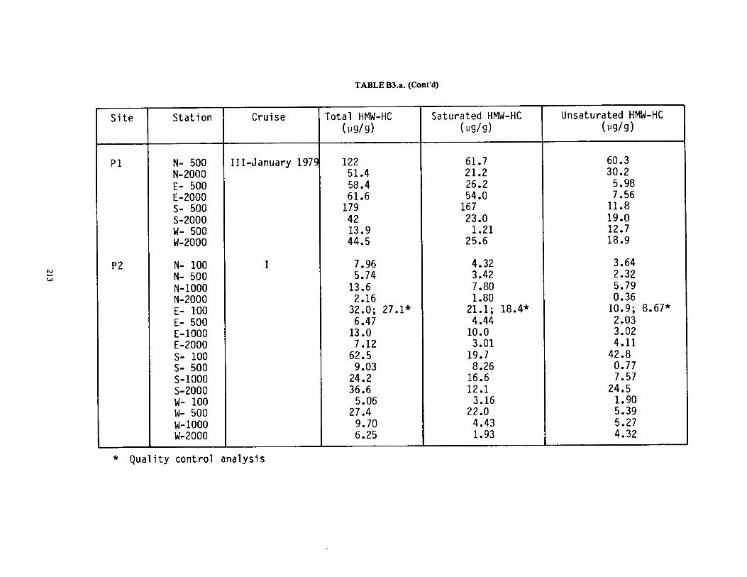
TABLE B3.a. (Cont'd)

N W

Site Station Cruise Total HMW-HC (u9/9)

Saturated HMW-HC (u9/9)

Unsaturated HMW-HC (u9/9)

P1 N- 500 III-January 1979 122 61 .7 60 .3 N-2000 51 .4 21 .2 30 .2 E- 500 58 .4 26 .2 5.98 E-2000 61 .6 54 .0 7.56 S- 500 179 167 11 .8 S-2000 42 23 .0 19 .0 W- 500 13 .9 1 .21 12 .7 W-2000 44 .5 25 .6 18 .9

P2 N- 100 1 7.96 4.32 3.64 N- 500 5.74 3.42 2.32 N-1000 13 .6 7.80 5.79 N-2000 2 .16 1 .80 0.36 E- 100 32 .0 ; 27 .1* 21 .1 ; 18 .4* 10 .9 ; 8.67* E- 500 6 .47 4 .44 2 .03 E-1000 13 .0 10 .0 3 .02 E-2000 7 .12 3 .01 4 .11 S- 100 62 .5 19 .7 42 .8 S- 500 9.03 8.26 0.77 S-1000 24 .2 16 .6 7 .57 S-2000 36 .6 12 .1 24 .5 W- 100 5 .06 3.16 1 .90 W- 500 27 .4 22 .0 5.39 W-1000 9 .70 4.43 5 .27 W-2000 6.25 1 .93 4 .32

* Quality control analysis

TABLE B3.a . (cont'd)

Site Station Cruise Total HMW-HC (ug/9)

Saturated HMW-HC (ug/9)

Unsaturated HMW-HC (ug/9)

P2 N- 500 II 14 .0 10 .3 3 .68 N-2000 15 .2 9.56 5 .67 E- 500 15 .0 9.72 5 .31 E-2000 32 .7 31 .4 1 .28 S- 500 14 .0 12 .2 1 .82 S-2000 -- -- -- W- 500 31 .6 28 .5 3.13 W-2000 13.9 8.99 4.93

P2 N- 500 III 4.51 1 .86 2.65 N-2000 25 .7 19 .6 6.14 E- 500 34 .2 25 .9 8.26 E-2000 35 .0 24 .1 10 .9 S- 500 24 .2 17 .3 6.94 S-2000 31 .0 23 .1 7.86 W- 500 16 .2 10 .3 5.90 W-2000 15 .4 1 .5 7.91

* Quality control analysis

TABLE B3.a . (cont'd)

Site Station Cruise Total HMW-HC (u9/9)

Saturated HMW-HC (u9/9)

Unsaturated HMW-HC (u9/9)

P3 N- 100 1 6 .85 4 .70 2 .15 N- 500 9.49 5 .53 3.96 N-1000 4 .64 3 .06 1 .58 N-2000 4 .74 3 .07 1 .67 E- 100 18 .2 ; 17 .7* 11 .7 ; 14 .0* 6 .51 ; 3.70* E- 500 8 .57 6 .28 2 .29 E-1000 6.16 3.33 2 .83 E-2000 9 .87 7 .61 2 .26 S- 100 9.98 7 .25 2.73 S- 500 11 .8 10 .63 1 .17 S-1000 10 .7 8.12 2.54 S-2000 7 .24 5 .44 1 .80 W- 100 14 .0 8 .64 5 .34 W- 500 11 .2 10 .4 0.75 W-1000 3 .69 2 .34 1 .35 W-2000 9.61 5.65 3 .96

P3 N- 500 11 20 .6 17 .6 2.99 N-2000 5 .30 4 .03 1 .27 E- 500 12 .3 ; 14 .5** 5 .22 ; 9.53** 7 .04 ; 4.95** E-2000 22 .9 16 .8 6.06 S- 500 16 .2 ; 11 .9** 11 .5 ; a.37** 4.74 ; 3.57** S-2000 46 .1 ; 26 .5** 38 .3 ; 17 .7** 7 .19 ; 8 .77** W- 500 13 .8 ; 6 .97** 12 .4 ; 5 .00** 1 .36 ; 1 .97** W-2000 14 .6 11 .0 3 .63

* Quality control analysis ** Sample collection repeated

TABLE B3.a . (conYd)

Site Station Cruise Total HMW-HC (u9/9)

Saturated HMW-HC (u9/9)

Unsaturated HMW-HC (u9/9)

P3 N- 500 III 18 .1 12 .2 5.85 N-2000 12 .1 7 .16 4.97 E- 500 10 .4 7 .06 3.34 E-2000 7 .69 4.56 3.13 S- 500 38 .3 32 .0 6.34 S-2000 13 .5 7 .81 5.12 W- 500 6.85 5 .71 1 .14 W-2000 9.78 7 .46 2.32

P4 N- 100 I 80 .9 7 .56 73 .3 N- 500 25 .0 9.59 15 .4 N-1000 26 .1 22 .4 3.74 N-2000 21 .6 15 .3 6.30 E- 100 15 .5 ; 9.79* 9.33 ; 6 .25* 6.13 ; 3.54* E- 500 26 .2 17 .4 8.81 E-1000 22 .3 16 .8 5.48 E-2000 30 .3 27 .1 3.21 S- 100 6.63 4.14 2.49 S- 500 24 .8 17 .0 7 .71 S-1000 40 .4 30 .3 10 .1 S-2000 7 .61 4.15 3.46 W- 100 -- __ -- W- 500 66 .4 60 .1 16 .30 W-1000 41 .2 26 .8 14 .4 W-2000 38 .1 26 .9 11 .2

* Quality control analysis

TABLE B3.a . (conYd)

N

v

Site Station Cruise Total HMW-HC (u9/9)

Saturated HMW-HC (u9/9)

Unsaturated HMW-HC (u9/9)

P4 N- 500 II 23 .6 14 .1 9.45 N-2000 19 .8 13 .3 6.51 E- 500 44 .4 29 .7 14 .7 E-2000 24 .2 16 .4 7 .79 S- 500 14 .3 9.46 4.88 S-2000 23 .1 12 .5 10 .6 W- 500 15 .2 10 .3 4.85 W-2000 -- -- '-

P4 N- 500 III 40 .2 31 .2 9.01 N-2000 18 .5 1.78 10 .7 E- 500 22 .4 19 .3 3.11 E-2000 26 .4 17 .5 8.87 S- 500 19 .1 14 .4 4.70 S-2000 30 .4 17 .9 12 .5 W- 500 5.58 2.85 2.73 W-2000 27 .1 12 .7 14 .4

S5 N- 100 II 25 .4 13 .3 12 .1 N- 500 41 .1 6.80 34 .3 N-1000 42 .0 36 .0 5 .98 N-2000 7 .59 3.90 3 .69

* Quality control analysis

TABLE B3.a . (conYd)

Site Station Cruise Total HMW-HC (u9/9)

Saturated HMW-HC (u9/9)

Unsaturated HMW-HC (u9/9)

S6 N- 100 II 102 .4 ; 67 .3* 69 .3 ; 54 .5* 33 .1 ; 12 .8* N- 500 148 ; 113* 37 .9 ; 22 .6* 111 ; 90 .4* N-1000 49 .1 26 .8 22 .3 N-2000 43 .5 3.34 40 .2

S7 N- 100 II 67 .8 24 .6 43 .2 N- 500 47 .5 30 .0 17 .5 N-1000 60 .2 47 .5 12 .7 N-2000 38 .6 28 .0 10 .6

S8 N- 100 II 34 .0 22 .4 11 .6 N- 500 21 .5 15 .0 6.48 N-1000 54 .1 32 .0 22 .1 N-2000 22 .8 2 .48 20 .3

S9 N- 100 II 13 .2 7 .95 5 .26 N- 500 19 .5 12 .0 7 .51 N-1000 39 .4 27 .1 12 .3 N-2000 50 .5 41 .3 9 .20

S10 N- 100 II 32 .3 7.67 24 .6 N- 500 3.95 1 .69 2 .26 N-1000 8.55 7 .95 0 .60 N-2000 24 .2 19 .49 4 .66

* Quality control analysis

TABLE B3.a. (cont'd)

Site Station Cruise Total HMW-HC (u9/9)

Saturated HMW-HC (u9/9)

Unsaturated HMW-HC (u9/9)

S11 N- 100 II 223 3 .21 220 N- 500 12 7 .30 4 .35 N-1000 7 .33 3.17 4.16 N-2000 14 .0 5 .23 8 .72

S12 N- 100 II 43 .6 7.91 35 .7 N- 500 18 .8 13 .1 5.70 N-1000 36 .9 29 .0 7.88 N-2000 15 .2 7.03 8 .12

S13 N- 100 II 105 79 .9 25 .2 N- 500 85 .0 ; 66 .1* 60 .1 ; 36 .6* 24 .9 ; 29 .5* N-1000 87 .3 46 .3 41 .0 N-2000 54 .4 24 .6 29 .8

S14 N- 100 II 64 .5 26 .9 37 .6 N- 500 37 .5 30 .2 6.95 N-1000 18 .9 14 .5 4 .42 N-2000 8.16 3.24 4 .92

S15 N- 100 II 38 .2 28 .1 10 .1 N- 500 23 .0 16 .9 6 .13 N-1000 29 .6 22 .6 7 .00 N-2000 23 .6 12 .1 11 .5

* Quality control analysis

TABLE B3.a . (cont'd)

Site Station Cruise Total HMW-HC (u9/9)

Saturated HMW-HC (u9/9)

Unsaturated HMW-HC (u9/9)

S16 N- 100 II 107 12 .1 94 .6 N- 500 84 .9 14 .5 70 .4 N-1000 55 .1 29 .6 25 .5 N-2000 49 .7 37 .5 12 .2

S17 N- 100 II 76 .3 12 .7 63 .6 N- 500 72 .7 ; 50 .4* 45 .2 ; 38 .2* 27 .5 ; 12 .2* N-1000 29 .6 13 .8 15 .8 N-2000 13 .6 9.68 3.94

S18 N- 100 II 41 .6 28 .3 13 .3 N- 500 75 .8 61 .2 14 .6 N-1000 10 .0 3.04 6.99 N-2000 30 .6 19 .3 11 .3

S19 N- 100 I I N- 500 3 .42 2 .02 1 .40 N-1000 8.25 4.87 3.38 N-2000 5 .47 2 .49 2.98

S20 N- 100 II 34 .9 28 .4 6.54 N- 500 7 .64 5 .53 2.11 N-1000 15 .4 11 .8 3.60 N-2000 4.70 2.07 2.63

Quality control analysis

TABLE B3.a. (cont'd)

Site Station Cruise Total HMW-HC (u9/9)

Saturated HMW-HC Ou9/9)

Unsaturated HMW-HC (u9/9)

C21 1 31 .8 27 .6 4.18 II 73 .5 34 .9 38 .6 III 38 .0 31 .2 6.78

C22 I 40 .2 17 .7 22 .5 II 23 .9 13 .3 10 .6 III 33 .8 23 .0 10 .8

C23 1 13 .5 10 .1 3.41 II 10 .4 10 .4 0.04 III 32 .6 29 .8 2.84

C24 1 45 .5 41 .5 4.00 II 32 .9 23 .5 9.40 III 45 .2 19 .1 26 .1

TABLE B3. High molecular weight hydrocarbons (HMW-HC) in surficial sediments. b. Average values .

Site Cruise HMW-HC HCI Total Saturated Unsaturated

P1 I 87 .4 33 .7 53 .7 II 94 .8 64 .4 30 .3 III 71 .6 47 .5 20 .8 Average 84 .5 2 .41

P2 I 17 .4 9.56 7.85 II 19 .5 15 .8 3.69 III 23 .3 16 .2 7 .07 Average 20 .1 0.57

P3 I 9.67 6.93 2.74 II 17 .6 13 .1 4 .51 III 14 .6 10 .5 4.10 Average 14 .0 0.40

P4 I 30 .2 18 .8 11 .4 II 23 .5 15 .1 8 .40 III 23 .7 15 .5 8.25 Average 25 .8 0.74

S5 II 29 .0 15 .0 14 .0 0.82

S6 II 87 .2 35 .7 51 .6 2 .48

S7 II 53 .5 32 .5 21 .0 1 .52

S8 II 33 .1 18 .0 15 .1 0.94

S9 II 30 .7 22 .1 8 .57 0.87

S10 II 17 .3 9 .2 8.03 0.49

S11 II 64 .1 4 .73 59 .3 1 .82

S12 II 28 .6 14 .3 14 .4 0.81

S13 II 79 .6 49 .5 30 .1 2 .26

S14 II 32 .2 18 .7 13 .5 0 .91

S15 II 28 .6 19 .9 8.68 0.81

S16 II 74 .2 23 .4 50 .7 2 .11

222

TABLE B3.b. (Cont'd)

Site Cruise HMW-HC HCI Total Saturated Unsaturated

S17 II 48 .5 23 .9 24 .6 . 1 .38

S18 II 39 .5 28 .0 11 .5 1 .12

S19 II 5 .71 3 .13 2 .59 0 .16

S20 II 15 .7 11 .8 3.72 0.45

X21 I 31 .8 27 .6 4.18 II 73 .5 34 .9 38 .6 III 38 .0 31 .2 6.78 Average 47 .8 1 .36

C22 I 40 .2 17 .7 22 .5 II 23 .9 13 .3 10 .6 III 33 .8 23 .0 10 .8 Average 32 .6 0.93

C23 I 13 .5 10 .1 3 .41 II 10 .4 10 .4 0 .04 III 32 .6 29 .8 2.84 Average 18 .8 0.54

C24 I 45 .5 41 .5 4.00 II 32 .9 23 .5 9 .40 III 45 .2 19 .1 26 .1 Average 41 .2 1 .17

223

TABLE B4 . High molecular weight hydrocarbons (HMW-HC) in downcore sediments.

Site Station Sample Interval (cm)

Total HMW-HC (ug/g)

Saturated HMW-HC (u9/9)

Unsaturated HMW-HC (u9/9)

P1 N-500 0-13 3 .77 3 .38 0 .39 13-26 7 .49 1 .19 6.30 26-39 27 .4 6.30 21 .1

P2 N-500 0-3 14 .0 5.14 8.86 3-13 14 .6 5.13 9.43

13-20 45 .7 10 .0 35 .7

P3 N-500 0-6 14 .0 13 .8 0.19 6-16 15 .3 11 .1 4.23

16-25 19 .0 15 .1 3.91 25-35 26 .1 21 .3 4.84

P4 N-500 0-20 8 .33 6 .23 2 .10 20-35 9 .37 7 .68 1 .69 35-47 15 .0 7 .89 7 .15

C21 N-500 0-10 10 .2 7 .31 2 .88 10-24 13 .9 2.98 10 .9 24-38 14 .6 12 .1 2 .47

C22 N-500 0-10 8 .39 4.80 " 59 10-20 10 .6 7 .63 2 .96 20-30 26 .4 23 .6 2 .80

C23 N-500 0-12 12 .3 9.38 2.94 12-24 13 .3 10 .5 2 .83 24-36 14 .1 11 .7 2 .40 36-52 14 .3 3 .1 11 .2

C24 N-500 0-10 0 .17 0.10 .07 10-20 0.78 0.70 0.08 20-30 10 .8 9.51 1 .27 30-40 23 .8 23 .7 0.05 40-50 0 .00 0.00 0.00

224

The Department of the Interior Mission As the Nation's principal conservation agency, the Department of the Interior has responsibility for most of our nationally owned public lands and natural resources. This includes fostering sound use of our land and water resources; protecting our fish, wildlife, and biological diversity; preserving the environmental and cultural values of our national parks and historical places; and providing for the enjoyment of life through outdoor recreation. The Department assesses our energy and mineral resources and works to ensure that their development is in the best interests of all our people by encouraging stewardship and citizen participation in their care. The Department also has a major responsibility for American Indian reservation communities and for people who live in island territories under U.S. administration. The Minerals Management Service Mission As a bureau of the Department of the Interior, the Minerals Management Service's (MMS) primary responsibilities are to manage the mineral resources located on the Nation's Outer Continental Shelf (OCS), collect revenue from the Federal OCS and onshore Federal and Indian lands, and distribute those revenues. Moreover, in working to meet its responsibilities, the Offshore Minerals Management Program administers the OCS competitive leasing program and oversees the safe and environmentally sound exploration and production of our Nation's offshore natural gas, oil and other mineral resources. The MMS Minerals Revenue Management meets its responsibilities by ensuring the efficient, timely and accurate collection and disbursement of revenue from mineral leasing and production due to Indian tribes and allottees, States and the U.S. Treasury. The MMS strives to fulfill its responsibilities through the general guiding principles of: (1) being responsive to the public's concerns and interests by maintaining a dialogue with all potentially affected parties and (2) carrying out its programs with an emphasis on working to enhance the quality of life for all Americans by lending MMS assistance and expertise to economic development and environmental protection.