ecological network indicators of ecosystem status and

Ecological Network Indicators of Ecosystem Status andChange in the Baltic SeaMaciej T. Tomczak1*, Johanna J. Heymans2, Johanna Yletyinen3,4, Susa Niiranen4, Saskia A. Otto4,

Thorsten Blenckner4

1 Baltic Sea Centre, Stockholm University, Stockholm, Sweden, 2 Scottish Association for Marine Science, Scottish Marine Institute, Dunbeg, Oban, United Kingdom,

3Nordic Centre for Research on Marine Ecosystems and Resources under Climate Change (NorMER), Stockholm Resilience Centre, Stockholm University, Stockholm,

Sweden, 4 Stockholm Resilience Centre, Stockholm University, Stockholm, Sweden

Abstract

Several marine ecosystems under anthropogenic pressure have experienced shifts from one ecological state to another. Inthe central Baltic Sea, the regime shift of the 1980s has been associated with food-web reorganization and redirection ofenergy flow pathways. These long-term dynamics from 1974 to 2006 have been simulated here using a food-web modelforced by climate and fishing. Ecological network analysis was performed to calculate indices of ecosystem change. Themodel replicated the regime shift. The analyses of indicators suggested that the system’s resilience was higher prior to 1988and lower thereafter. The ecosystem topology also changed from a web-like structure to a linearized food-web.

Citation: Tomczak MT, Heymans JJ, Yletyinen J, Niiranen S, Otto SA, et al. (2013) Ecological Network Indicators of Ecosystem Status and Change in the BalticSea. PLoS ONE 8(10): e75439. doi:10.1371/journal.pone.0075439

Editor: Brian R. MacKenzie, Technical University of Denmark, Denmark

Received February 26, 2013; Accepted August 15, 2013; Published October 7, 2013

Copyright: � 2013 Tomczak et al. This is an open-access article distributed under the terms of the Creative Commons Attribution License, which permitsunrestricted use, distribution, and reproduction in any medium, provided the original author and source are credited.

Funding: The study has been carried out with financial support from the EU 7th Framework Project KnowSeas (FP7/2007–2013) under grant agreement number226675 and the Swedish FORMAS project ‘‘Regime Shifts in the Baltic Sea Ecosystem-Modelling Complex Adaptive Ecosystems and Governance Implications’’.Further, the research leading to these results has received funding from the Baltic Ecosystem Adaptive Management (BEAM) program funded by SwedishFORMAS, and from the Norden Top-level Research Initiative sub-programme ‘Effect Studies and Adaptation to Climate Change’ through the Nordic Centre forResearch on Marine Ecosystems and Resources under Climate Change (NorMER). The funders had no role in study design, data collection and analysis, decision topublish, or preparation of the manuscript.

Competing Interests: The authors have declared that no competing interests exist.

* E-mail: [email protected]

Introduction

Many marine ecosystems are under pressure due to multiple

drivers, such as fishing, climate change and eutrophication,

causing large-scale food-web reorganizations, often called regime

shifts [1]. The definitions of regime shifts vary, see for example

Lees et al. [1]. In this study, we use the definition of McKinnell

et al. [2] who state that: ‘‘regime shifts are low-frequency, high-

amplitude and sometimes abrupt changes in species abundance,

community composition and trophic organization that occur

concurrently with physical changes in the climate system’’.

McKinnell et al. [2] and Cury and Shannon [3,4] highlight

changes of the internal structure, organization and size of an

ecosystem as characteristic of regime shifts. Regime shifts have

been described in several marine ecosystems such as the Southern

and Northern Benguela [3,5,6], Southeast Alaska and Aleutian

Islands [7] and the Black Sea [8]. All of these regime shifts have

the re-organisation of food-webs in common. In general, food-web

re-organizations are best described by Ecological Network

Analysis (ENA) sensu Ulanowicz [9]. The network approach to

ecological research provides a powerful representation of the

pattern of interactions among species; highlights their interdepen-

dence and equips ecologists to find generalities among seemingly

different systems [10]. Knowledge of the network topology (e.g.

connectance, number of species, interaction rates) provides

insights to ecosystem functioning and stability, highlights the

advantages of integrating network research with empirical

indicators of resilience, and uncovers generic features of these

complex systems [10–16].

In the Baltic Sea (Fig. 1), an ecosystem regime shift has been

described for the Central Basin (Baltic Proper) in the late 1980s

[17,18]. This regime shift included pronounced changes and

reorganizations within and across the trophic levels of zooplankton

and fish [17,18]. Network analyses have already been applied to

the Baltic Sea. For example, Wulff et al. [19] used the ENA

method to compare the Baltic Sea to Chesapeake Bay and

Tomczak et al. [20] used ENA to compare coastal ecosystem

maturation and stress in five coastal ecosystems. However, none of

these Baltic related ENA studies took temporal changes in the

ENA indices and regime shifts into account. Similarly, a number

of studies have analysed food-web changes in other marine systems

using ENA indices [4,5,21–23], but very few have used a time

dynamic approach [7].

Thus, we focused on changes in the resilience of the Baltic

ecosystem to describe and understand the processes underlying the

regime shift. We investigated food-web reorganisation at the

ecosystem level as revealed by the theory of ecological succession

and maturity [9,24,25], which is linked to the theory of resilience

[26] and regime shifts [27,28]. Therefore, the aim of this study was

to calculate temporally integrated ENA and ecological indices to

test for dynamic changes in the food-web in relation to the

suggested regime shift, and to explain these changes in relation to

the resilience and trophodynamic properties of the Baltic Sea

ecosystem.

PLOS ONE | www.plosone.org 1 October 2013 | Volume 8 | Issue 10 | e75439

Materials and Methods

Study SiteThe Baltic Sea hydrographical conditions are characterized by:

(i) a horizontal sea surface salinity gradient from 10 PSU in the

South-West to 6 PSU in the North-Eastern part of the Baltic

Proper [29], (ii) high riverine inflows [30], and (iii) major,

irregular, inflows of saline, oxygenated water from the North

Sea leading to a permanent pycnocline that partly contributes to

deep-water hypoxia [31,32]. During the last century, high land-

based nutrient loads have led to the eutrophication of the Baltic

Sea with typical eutrophication-related symptoms, such as massive

cyanobacteria blooms in summer and widespread deep-water

anoxia [31,33].

Fisheries have heavily exploited the Baltic Sea resources [34].

Landings of the main commercial fish stock, Eastern Baltic cod

(Gadus morhua calarias), increased dramatically at the beginning of

the 1980s and collapsed in the early 1990s [35]. During that time

cod biomass has declined severely [36]. Instead, small pelagic fish,

such as sprat (Sprattus sprattus) and herring (Clupea harengus), have

dominated the catches during the last 20 years [35]. Mollmann

et al. [18] suggested that high fishing pressure on cod contributed

to its decline, and the resulting trophic effects cascaded down to

the copepods (Pseudocalanus acuspes). Increasing temperature

positively affected zooplankton (Acartia spp.) abundance, sprat

reproduction, and consequently established the current regime of

Acartia spp. and sprat dominance [37].

Modelling Approach and Model DescriptionEcopath with Ecosim [38] was created for building food-web

models (www.ecopath.org). The dynamic extension of Ecopath

that allows temporal analysis and fitting the model to time series is

undertaken by Ecosim, using the master equation (1)

dBi=dt~giX

j

Qji{X

QjizIi{ M0izFzeið Þ.Bi ð1Þ

where dBi/dt represents the growth rate during the time interval

dt of group (i) in terms of its biomass (Bi), gi is the net growth

efficiency (production/consumption ratio), Qji is the consumption

rates, M0i the non-predation (‘other’) natural mortality rate, Fi is

fishing mortality rate, ei is emigration rate, Ii is immigration rate

(and ei*Bi-Ii is the net migration rate).

The current Baltic Ecopath with Ecosim model, based on

Tomczak et al. [39], covers the area of the Central Baltic Sea

(ICES subdivisions 25–29, excluding Gulf of Riga) and contains 21

functional groups (Fig. 2), including three fishing fleets on the main

commercial fish species: cod, sprat and herring. For details see

Tab. S1–S3 and Fig. S1–S3 in File S1.

Data and AnalysisThree analyses were performed to: i) test for abrupt changes in

the observed data that were used to force the ecosystem model, ii)

test for abrupt changes in the modelled biomass, and iii) analyse

ecosystem properties (ENA indices) in reference to observed

changes [18], and the ecological theories of Scheffer and

Carpenter [28], Folke et al. [40] and Odum [24] (see section

Linking theory).

Forcing Data and Simulated BiomassThe forcing data represent both environmental and human

impacts on the Baltic Sea food-web (Fig. S2 in File S1). Temporal

anomalies of sea surface temperature in August and the spring

temperature from 0–50 m depth (SST_aug; TempWC_spring),

primary production (PP_BALTSEM), hypoxic area, Cod Repro-

ductive Volume (CodRV [41]), herring recruitment (HER_rec), as

well as fishing on small and adult cod (FSmallCod, FAdCod), sprat

(FJuvSprat, FAdSprat) and herring (FJuvHerr, FAdHerr) were

analysed to test for non-linear shifts. For the time series data used

see references and application details in Tomczak et al. [39]. The

modelled biomasses of 19 of the 21 functional groups were

included in the statistical analysis (see section Statistical analysis

and Fig. S3 in File S1). Seals and detritus were excluded from the

dataset to ensure that the data were comparable and consistent

with the number of trophic levels used in Mollmann et al. [18]. A

further motivation for exclusion of the seal and detritus data was

that seal biomass was used as one of the forcings in the model,

while detritus showed very high cross-correlation with PP.

Ecosystem Indicators and Ecological Network AnalysisIndicesWe calculated 15 network analysis indices, ecosystem metrics

and biomass diversity indices (Fig. 3; for definitions and

descriptions see Tab. S5 in File S1), commonly used to describe

changes in ecosystem properties and food-web dynamics

[7,9,19,21,22,24,25,42–54]. Indices were assigned to a number

of groups, describing ecosystem properties in terms of ecosystem/

food-web resilience and structure, and fisheries. Structure indices

included: Total System Throughput (TST), Relative Ascendancy

(A/C), Redundancy (R), Average Mutual Information (AMI),

Entropy (H), Mean Path Length (MPL), Kempton-Q index (Q),

recycling within the ecosystem: Finn Cycle Index (FCI), Predatory

Cycle Index (PCI), Proportional Flow to Detritus (PFD), System

turnover rate (ToTP/ToTB), and Total Primary Production per

Total Respiration (TPP/TR). Fisheries impact indices included:

Primary Production Required to sustain catch per Primary

Production (PPR/PP), mean Trophic Level of catch (mTLc), and

Total Catch (Tot C).

Figure 1. The Baltic Sea with the study area, the Baltic Proper(dark).doi:10.1371/journal.pone.0075439.g001

Ecological Indicators of Baltic Sea Ecosystem


Linking TheoryMageau et al. [25] used ENA indices to define system health

[55] and maturation [43] and concluded that an unstressed

(healthy) ecosystem is able to maintain its structure (organization)

and function (vigor) over time in the face of external stress

(resilience). Vigor is a measure of system activity, metabolism or

production [55]. Organization is a measure of the number and

diversity of interactions between the components of a system, and

resilience refers to the ability of a system to maintain its structure

and function in the presence of stress [25]. Odum [56] and

Ulanowicz [9] suggested that stressed ecosystems are characterized

by an inhibition or even reversal of the trends associated with

ecosystem development. In this paper we specifically refer to

proxies of resilience - namely redundancy (Tab. S5 in File S1),

linked by Christensen [43] with system stability and proposed by

Heymans et al. [7] as an index of food-web resilience. According to

Bondavalli et al. [57] high redundancy signifies that either the

system is maintaining a higher number of parallel trophic channels

in order to compensate for the effects of environmental stress, or

that it is well along its way to maturity. At the same time, Scheffer

et al. [27] and Scheffer and Carpenter [28] defined resilience as

the ‘‘depth of the basin of attraction’’. We link resilience to

changes in redundancy, by assuming that R is a proxy of resilience

as given by Christensen [43] and Heymans et al. [7].

Statistical AnalysisA series of statistical methods (see sections below) as described in

Diekmann and Mollmann [58] were applied to the time series of

model forcing (force) and modelled biomass (mb): 1) Sequential t-

test analyses of regime shifts (STARS) [59]; 2) Principal

Component Analysis (PCA); 3) STARS on PCA scores and 4)

Chronological Clustering Analysis (CC) [60]. Due to high cross-

correlations (see Tab. S6 in File S1), we did not perform a PCA on

the ENA indices. Instead, ENA indices were analysed using

STARS and integrated using CC. For ENA indices, coefficient of

variation (CV) was estimated to examine the variability in the

given time periods. A traffic light plot was used to visualise the

dynamics of subsequent data sets (forcing and biomass).

Sequential t-test Analyses of Regime Shifts (STARS)To recognize significant shifts in mean values of a given time

series, a sequential t-test on the mean (STARS) was applied for

each time series separately. The two parameters that control the

scale and magnitude of potential regime shifts were set a priori. The

significance level (a) was set to 0.05. The cut-off length (l) was set to

five for forcing variables and indices, to test for changes in ‘‘fast’’

environmental variables and examine specific periods of changes

between regimes. For modelled biomasses, the cut-off length was

set to 10 years for comparison to Mollmann et al. [18]. The

calculation of shifts was also affected by the handling of outliers.

Thus, the Huber’s weight parameter (which controls the

identification and weights assigned to outliers [59]) was set to 3.

Figure 2. The structure of the food-web model, also indicating the fishing pressure (F) for the respective fisheries on the three fishspecies, pp – primary producers, juv – juvenile stanza of given fish species. Detritus pool is divided into two groups: detritus on thesediment (detritus (s)) and water column detritus (detritus (w)).doi:10.1371/journal.pone.0075439.g002



Therefore, if the deviation of a measurement from the expected

average (normalized by its standard deviation) was .3, its weight

was inversely proportional to the distance from the expected mean

value. Shifts detected in the very last years were not taken into

account during the analysis due to the known limitation of this

method [61].

Principal Component Analysis (PCA)Standardized PCA, based on the correlation matrix, was carried

out on the transformed values (ln+1) of the given data set. First, a

PCA was applied for forcing (force) and modelled biomass (mb)

time series. The PC1 scores on the forcing variables (PC1force)

were used as an index of pressure and the scores of the modelled

Figure 3. Ecological indicators and ENA indices anomalies (note different scale) from 1974–2006.doi:10.1371/journal.pone.0075439.g003



biomass were used as an index of biological change (PC1mb).

Annual scores of the two principal components, PC1mb and

PC2mb, were plotted against time to visualise temporal relation-

ships and the occurrence of abrupt modelled system changes.

Variable loadings and scores were displayed on the 1st factorial

plane, and the years were chronologically connected to show the

pressure/state trajectory [18].

STARS on PCA Index Time SeriesSTARS were used to detect sudden changes in the PC scores to

identify whether abrupt changes had occurred [18]. Parameters

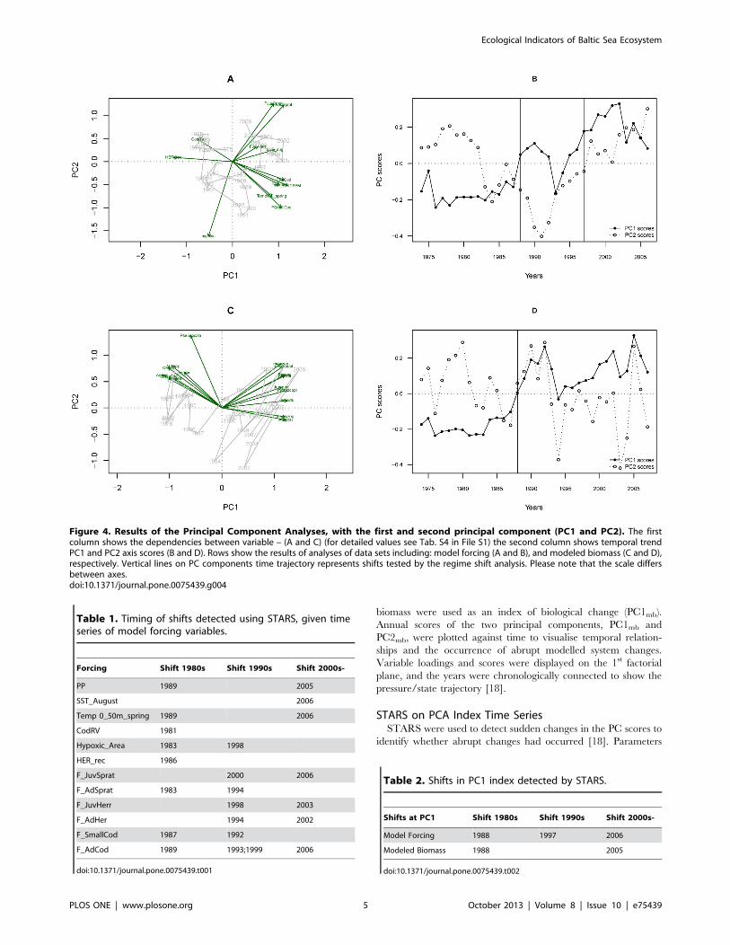
Figure 4. Results of the Principal Component Analyses, with the first and second principal component (PC1 and PC2). The firstcolumn shows the dependencies between variable – (A and C) (for detailed values see Tab. S4 in File S1) the second column shows temporal trendPC1 and PC2 axis scores (B and D). Rows show the results of analyses of data sets including: model forcing (A and B), and modeled biomass (C and D),respectively. Vertical lines on PC components time trajectory represents shifts tested by the regime shift analysis. Please note that the scale differsbetween axes.doi:10.1371/journal.pone.0075439.g004

Table 1. Timing of shifts detected using STARS, given timeseries of model forcing variables.

Forcing Shift 1980s Shift 1990s Shift 2000s-

PP 1989 2005

SST_August 2006

Temp 0_50m_spring 1989 2006

CodRV 1981

Hypoxic_Area 1983 1998

HER_rec 1986

F_JuvSprat 2000 2006

F_AdSprat 1983 1994

F_JuvHerr 1998 2003

F_AdHer 1994 2002

F_SmallCod 1987 1992

F_AdCod 1989 1993;1999 2006

doi:10.1371/journal.pone.0075439.t001

Table 2. Shifts in PC1 index detected by STARS.

Shifts at PC1 Shift 1980s Shift 1990s Shift 2000s-

Model Forcing 1988 1997 2006

Modeled Biomass 1988 2005




for the analyses were set as described in sections above.

Chronological Clustering (CC)Independently of the STARS and PCA analyses, a second

discontinuity analysis, CC, was carried out to identify the years in

which the largest shifts in the mean value of the time series

occurred. This method groups sequential years based on a time-

variable matrix [61]. To demonstrate the most important break-

points in the dataset, the significance level (a), which can be

considered as a clustering-intensity parameter, was set to 0.01. The

connectedness level was set to 50%. In accordance with the use of

the correlation coefficient in the PCA, the data were first

normalized, and then the Euclidean distance was calculated to

determine similarity between years.

Traffic Light Plots (TLP)To visualise overall systematic patterns based on single time

series, TLPs were generated [62]. The modelled biomass values of

each functional group were categorized into quintiles and each

quantile was assigned a specific colour: green for the lowest (0–

20%), red for the highest (80–100%) and a gradation of colours in

between. The variables were then sorted in descending order

according to their PC1 loadings, and plotted against years to

visualise temporal patterns.

Results

Changes in External ForcingMany of the observed changes in model forcing time series

(Tab. 1) occur in the mid-late 1980s and mid-late 1990s, with some

shifts appearing after 2000 (Fishing mortality of Juv. Sprat, Juv.

Herring and Adult Herring). PCA on the forcing time series (Fig. 4)

indicates a strong change in the overall pressure on the ecosystem

(Fig. 4A) with changes in PC1force and PC2force indices (Fig. 4B)

explaining 33% and 18% of the total variation, respectively.

Forcing variables that contributed most to PC1force were: PP, Cod

RV, herring recruitment and the fishing mortality on cod and

sprat (Fig. 4A, Tab. S4 in File S1). The shifts in the forcing index

(i.e., PC1force) occurred in 1988 and 1997 (Fig. 4B, Tab. 2) while

CC detected data discontinuity at 1983, 1998 and 2003 (Tab. 3).

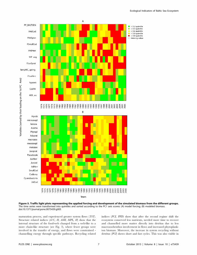
The traffic light plot (Fig. 5) illustrates the temporal changes in

forcing factors as well as modelled biomass: Fig. 5A shows

differences before (low PP, high Cod RV and low fishing) and after

the mid-1980s regime shift (with high PP suggesting eutrophica-

tion, high fishing, increased temperature and unfavourable cod

reproduction conditions).

Biomass State ChangeThe majority of significant shifts in modelled biomass occurred

in the late 1980s (Tab. 4), with three time series showing additional

shifts in the 1990s (Pseudocalanus sp., Juvenile Herring and Adult

Herring). The first two axes of the PCA on the modelled biomasses

(PC1mb and PC2mb; Fig. 4C and D, Tab. S4 in File S1) explained

72% and respectively 10% of the total variance. The shift in

biomass index (PC1mb, Fig. 4D) occurred in 1988, and is

confirmed by the CC (Tab. 3). The PCmb shifts (Tab. 2) and

traffic light plot of modelled biomass (Fig. 5B) shows a clear

dichotomy in the food-web, between cod vs. sprat and zooplank-

ton vs. plankton (Fig. 5B).

Emergent Food-web ChangesSimilar to findings from the forcing and biomass time series,

STARS detected shifts in most ecosystem descriptors and ENA

indices at the end of the 1980s (1987/89) and the mid-1990s

(1993/96) (Tab. 5). The ENA clearly shows two regimes, with a

discrete step function between the end of the 1980s and the mid-

1990s, described by Mollmann et al. [18] as a transitional period.

No significant shifts were detected in AMI, turnover rate (ToTP/

ToTB) or total primary production to respiration (TPP/TR), but

the anomalies for almost all indicators fluctuated significantly

(Fig. 3), showing extreme values between 1988 and 1995, and

increased variability (higher CV) after the late 1980s (Tab. 6).

Fisheries Affect Indicator ChangesIndicators directly related to exploitation reflect the shift in

fisheries both in total yield and catch composition (Fig. 3 and

Tab. 5). The first regime was characterized by high mTLc. The

second regime had high total catch dominated by sprat, decreasing

mTLc and increasing PPR/PP after the mid-1990s.

Resilience and Regime ShiftThe changes in redundancy (R) show a shift in 1989 and 1994

(Fig. 6). After 1994 a slight increase in R occurred, although not to

the high values of the pre-1988 phase. The decrease in the R after

the 1989 regime shift and the increase in 1994 indicate a transition

period with lowest resilience between the two regimes (regime I,

1974–1989 and regime II 1994–2006). Using our resilience index

– R as an index for ecosystem state and relating it to pressure

indices using PC1force shows the shift between the two regimes and

the transition period (Fig. 7). Between 1974 and 1988 the R

suggests a higher resilience, but with the change in the species

interaction and the multiple pressures, changing via a transition

period into another regime. The years 1992 and 1993 were

characterised by a low R, even though pressure was decreasing.

After 1993, R increased again, but not to the initial level, staying

constant even with a change in the pressure until about 2000 after

which it started to decline again.

Discussion

This study demonstrated that i) the regime shift in the Baltic Sea

in the late 1980s is well reflected by the ENA indices, and ii) two

different ecosystem regimes can be distinguished. The first regime

between 1974 and 1988 reflected a more mature and balanced

ecosystem, with more diverse flow structure, higher resilience,

characterised also by high primary production, and high fishing

pressure at relatively high trophic levels. The second regime,

between 1994 and 2006, was characterised as a more stressed, less

resilient regime with high primary production and high fishing

pressure on lower TL species, indicating a more productive and

linearized food-web. We hypothesise that the regime shift was

caused by the interplay of multiple drivers: climate, eutrophication

and fishing.

The macro descriptors (A/C, H, MPL) and food-web indices

(PCI, FCI, PFD) indicate that after the regime shift (mid-1990) the

ecosystem was more disturbed, more stressed, had an inverted

Table 3. Shifts in given data sets detected by ChronologicalClustering.

CC alfa = 0.01 Shift 1980s Shift 1990s Shift 2000s-

Model Forcing 1983 1998 2003

Modeled Biomass 1988

Modeled Indices 1989




maturation process, and experienced greater system flows (TST).

Structure related indices (A/C, H, AMI, MPL, H) show that the

internal structure of the food-web changed from a web-like to a

more chain-like structure (see Fig. 3), where fewer groups were

involved in the transfer of energy, and flows were constrained -

channelling energy through specific pathways. Recycling related

indices (FCI, PFD) show that after the second regime shift the

ecosystem conserved less nutrients, needed more time to recover

and channelled more matter directly into detritus due to less

macrozoobenthos involvement in flows and increased phytoplank-

ton biomass. Moreover, the increase in system recycling without

detritus (PCI) shows short and fast cycles. This was also visible in

Figure 5. Traffic light plots representing the applied forcing and development of the simulated biomass from the different groups.The time series were transformed into quintiles and sorted according to the PC1 axis scores: (A) model forcing; (B) modeled biomass.doi:10.1371/journal.pone.0075439.g005



the ecosystem turnover rate and Q index, which is due to the

higher proportion of biomass of small, fast growing organisms in

the food-web (i.e. sprat and small copepods) after the mid-1990s.

The changes in fisheries indicators during the first regime could

be explained by a higher percentage of cod in the catches, and low

PPR/PP, due to higher support of cod biomass from the detrital

food-chain [39]. The second regime was characterised by

increased sprat catches and the redirection of flows from benthic

to pelagic pathways [39]. According to Tudela et al. [65], PPR/PP

in combination with mTLc could be treated as an ecosystem index

to capture the effect of fisheries and define ‘‘Ecosystem Overfish-

ing’’. After the regime shift there was an increase in PPR/PP and a

drastic shift to lower mTLc. Therefore, this together with the

trends/shift described above suggest ecosystem overfishing in the

Baltic Sea.

A transition period, defined as the time when the ecosystem

changed from one regime to another, was suggested by the low R

between 1989 and 1993. It was characterized by high fluctuations

of ecosystem structure (AMI, Fig. 3) and flows (PCI, FCI, ToTP/

TotB or TPP/TR, Fig. 3), with the lowest system resilience (R, Fig. 7)

during the studied time period. The transition occurred where the

ecosystem was under high, constant pressure from eutrophication

and cod and herring fisheries (Fig. 7). However, at the same time

there was a stochastic overlap of hydrodynamic drivers, i.e.,

temperature, low cod reproductive volume (CodRV), probably

affecting the change (Fig. S2 in File S1, see also Lindegren et al.

[63]). After the transition period our analysis suggests that the

system did not return to the initial regime when the external

forcing was reduced.

Our ENA analysis suggests further that the resilience of the

second regime is lower than the first, and therefore another

significant disturbance of the ecosystem may cause the system to

move to another alternative regime [27] similar to what happened

in the Black Sea [64]. At this stage we are not able to say if the

current regime is reversible or how stable it is. However, since

2006 higher cod biomass seems to suggest a possible change

towards the first state [65].

Our results of forcing (abiotic factors) are in line with Mollmann

et al. [18,37] and the ICES Working Group on Integrated

Assessment of the Baltic Sea (WGIAB) [60]. It also agrees with

that of Kenny et al. [66] who showed a drivers shift in the 1980s

for the North Sea. The second shift, during the mid-1990s (Tab. 2),

has also been described by Mollmann et al. [18], although a similar

shift was not detected by Kenny et al. [66] for the North Sea. In

the mid-1980s, the North Atlantic Oscillation (NAO) and Baltic

Sea Index (BSI) shifted sharply from a negative to a positive phase,

Table 4. Timing of shifts detected using STARS, given timeseries of modeled biomass.

Modeled group Shift 1980s Shift 1990s Shift 2000s-

Cyanobacteria 1988 2006

Phytoplankton 1988

Microzooplankton 1988

Temora sp. 1988 2005

Acartia sp. 1988

Pseudocalanus sp. 1991

Mesozooplankton 1988 2005

Mysids 1988 2005

Meiozoobenthos 1988 2005

Macrozoobenthos 1988 2005

Juvenile Sprat 1988

Adult Sprat 1989 2006

Juvenile Herring 1994

Adult Herring 1982 1997

Cod larvae 1986

Juvenile Cod 1982

Small Cod 1984

Adult Cod 1985


Table 5. Timing of shifts detected using STARS, given timeseries of indices.

Indices Shift 1980s Shift 1990s Shift 2000s-

TST 1989 1994 2005

A/C 1993

R 1989 1994 2005

AMI

H 1988 2005

FCI 1988 2005

PCI 1993 2006

MPL 1988 2005

PFD 1989 2006

ToTP/TotB

TPP/TR 2005

Tot C 1983; 1988 1995 2005

PPR/PP 1996

mTLc 1982; 1987 1992

Kempton Q index 1979;1984;1989 1994 2002


Table 6. Coefficient of variation of used indices for giventime period (regime).

CV 1974–89 1990–2006 1974–2006

TST 0.108 0.148 0.215

A/C 0.007 0.014 0.014

R 0.013 0.017 0.031

AMI 0.012 0.022 0.018

H 0.006 0.011 0.015

PCI 0.160 0.310 0.318

FCI 0.097 0.144 0.188

MPL 0.035 0.033 0.061

PFD 0.014 0.017 0.030

ToTP/TotB 0.040 0.076 0.065

TPP/TR 0.022 0.045 0.039

Tot C 0.159 0.177 0.290

PPR/PP 0.183 0.244 0.285

mTLc 0.011 0.007 0.017

Kempton Q index 0.185 0.135 0.308




affecting the hydrodynamic conditions, i.e. temperature, salinity

and oxygen conditions throughout the whole area [64]. These

climate anomalies most probably induced the simultaneous regime

shift observed in the North Sea and Baltic Sea between 1987 and

1988 [17,63].

Despite the fact that the model reproduces shifts in given

functional groups relatively well (see Fig. S1 in File S1), and that

the integrated analyses (Tab. 2–3 and Fig. 4–5) compare well to

the results in Mollmann et al. [18], we are aware of the limitations

of our analyses, such as high cross-correlation, the lack of

seasonality and natural noise, as well as the aggregated and

simplified food-web structure.

Method DiscussionRecent advances in network science have encouraged ecologists

to study food-webs through network indices [14,67,68]. The

estimations of species interactions often benefit the understanding

of ecosystem response to perturbations [10,69], but it must be kept

in mind that the impact of network structure on community may

differ between different interaction types [70]. Consequently, the

ENA analysis depends strongly on model quality and structure. As

explained by Abarca-Arenas and Ulanowicz [71] and Pinnegar

et al. [72] the number of functional groups and model structure

have an impact on the number of flows and system properties.

This has to be taken into account when comparing our results to

other system outputs and other Baltic Sea models. Ecopath with

Ecosim [73] is a commonly used approach that has been broadly

discussed. Plaganyi and Butterworth [74], Aydin [75], Coll et al.

[76] and Walters et al. [77] described the pros and cons of the

methodology, which has been taken into account during model

building, fitting and evaluation [39,78]. Niiranen et al. [78] found

that data uncertainties may translate to uncertainties in modelled

trophic control and hence results. However in this study the model

was well fitted for several trophic levels and we have confidence in

the model and data [39], which represent changes in biomasses

and ecosystem dynamics well (see Fig. S1 in File S1).

Management OutlookOur results have significant implications for the understanding

of the dynamics of the ecosystem [40,79] and adaptive manage-

ment [80].

With regard to overall performance and robustness, ecosystem

level indicators based on ENA and food-web analysis are

informative on intermediate and long time-scales [4,81,82]. But

they are also difficult to use in annual updates of integrated

assessments and advice, and may be more difficult for stakeholders

to understand [82]. Nevertheless, examples of operational use do

exist, e.g. the Puget Sound Integrated Ecosystem Assessment [83].

In addition, using food-web models and the ENA approach to

explore different management scenarios, through changing fishing

mortality of different species, nutrient loads, and/or hydrodynam-

ic condition, could enable optimal management to ensure

restoration, increasing ecosystem resilience and guard against

future surprises.

Conclusions

Our study revealed that the cumulative nature of anthropogenic

stressors, such as fishing and eutrophication, needs to be analysed

in combination with large scale environmental drivers (climate),

ecosystem characteristics and emergent properties. This encapsu-

lates the holistic approach needed for ecosystem based manage-

ment. This is the first study where an abrupt regime shift was

demonstrated by using an index of resilience calculated from the

ecological network analysis using an Ecopath with Ecosim model

that described the system as a whole.

Supporting Information

File S1 Figure S1, Model fit to observed data (dots are

observations, solid line are model estimates). The input data

(annual biomass - B and cathes - C) and model estimates are

expressed as t/km2 of wet weight. Figure S2, Model forcing

anomalies relative to the initial value in 1974, 1974–2006 (note

different scale). Where SST_aug is sea surface temperature in

August; TempWC_spring is 0–50 m temperature in spring,

PP_BALTSEM represents primary production, hypoxic is the

area that is hypoxic, CodRV - Cod Reproductive Volume,

HER_rec is herring recruitments anomalies, FSmallCod and

FAdCod are anomalies of fishing morality of small and adult cod,

FJuvSprat and FAdSprat, FJuvHerr, FAdHerr represent fishing

mortality changes for adult and juvenile clupeid species. Figure S3,

Modelled biomass anomalies (note different scale) 1974–2006.

Figure 6. Time dynamics of redundancy (R) as percentage ofcapacity (C) in black and the red line represents the regimetested by the regime shift analysis for the period 1974–2006.doi:10.1371/journal.pone.0075439.g006

Figure 7. The redundancy (R) versus the overall pressure index,which is the principal component 1 from the model forcingvariables.doi:10.1371/journal.pone.0075439.g007



Table S1, Basic input to current EwE model (biomass is in t/km2,

P/B and Q/B are annual ratios of production and consumption to

biomass, EE is ecotrophic efficiency (proportion), P/Q is the ratio

of production to consumption, TL is trophic level and the catch is

in t/km2/yr. Table S2, Diet (proportion) composition matrix of

used EwE model. Table S3, Vulnerabilities parameters obtained

after model fitting. Table S4, PCA (PC1 and PC2) loadings - for

graphic representation see Figure 4A and 4C. Table S5, Indices

and definitions used. Table S6, Cross-correlations between indices.

(DOCX)

Acknowledgments

We would like to thank Dr. Karen Alexander from SAMS in Oban and

two anonymous reviewers for useful comments and language corrections

and Erik Smedberg from Baltic Nest Institute for graphical support.

Author Contributions

Conceived and designed the experiments: MTT JJH JY SAO TB.

Performed the experiments: MTT JJH SAO TB. Analyzed the data: MTT

JJH JY TB. Contributed reagents/materials/analysis tools: MTT JJH JY

SN SAO TB. Wrote the paper: MTT JJH JY SN SAO TB.

References

1. Lees K, Pitois S, Scott C, Frid C, Mackinson S (2006) Characterizing regimeshifts in the marine environment. Fish Fish 7: 104–127.

2. McKinnell SM, Brodeur RD, Hanawa K, Hollowed AB, Polovina JJ, et al.(2001) An introduction to the Beyond El Nino conference: climate variability

and marine ecosystem impacts from the tropics to the Arctic. Prog Oceanogr 49:1–6.

3. Cury P, Shannon L (2004) Regime shifts in upwelling ecosystems: observedchanges and possible mechanisms in the northern and southern Benguela. Prog

Oceanogr 60: 223–243.

4. Cury PM, Shannon LJ, Roux JP, Daskalov GM, Jarre A, et al. (2005)

Trophodynamic indicators for an ecosystem approach to fisheries. ICES J Mar

Sci 62: 430–442.

5. Shannon LJ, Field JG, Moloney CL (2004) Simulating anchovy-sardine regime

shifts in the southern Benguela ecosystem. Ecol Modell 172: 269–281.

6. Watermeyer KE, Shannon LJ, Griffiths CL (2008) Changes in the trophicstructure of the southern Benguela before and after the onset of industrial

fishing. Afr J Mar Sci 30: 351–382.

7. Heymans JJ, Guenette S, Christensen V (2007) Evaluating network analysis

indicators of ecosystem status in the Gulf of Alaska. Ecosystems 10: 488–502.

8. Daskalov GM, Grishin AN, Rodionov S, Mihneva V (2007) Trophic cascades

triggered by overfishing reveal possible mechanisms of ecosystem regime shifts.

Proc Natl Acad Sci USA 104: 10518–10523.

9. Ulanowicz R (1986) Growth and development: ecosystems phenomenology.

New York: Springer. 220 p.

10. Bascompte J (2009) Disentangling the Web of Life. Science 325: 416–419.

11. O’Gorman EJ, Emmerson MC (2009) Perturbations to trophic interactions and

the stability of complex food webs. Proc Natl Acad Sci USA 106: 13393–13398.

12. Dunne J, Brose U, Williams R, Martinez N (2005) Modeling food-web

dynamics: complexity-stability implications. In: Belgrano A, Scharler SU, Dunne

J, Ulanowicz RE, editors. Aquatic Food Webs An Ecosystem Approach. NewYork: Oxford University Press Inc. 117–129.

13. Martinez N, Williams R, Dunne J (2006) Diversity, complexity and persistencein large model ecosystems. In: Pascual M, Dunne J, editors. Ecological

Networks: Linking Structure to Dynamics in Food Webs. New York: OxfordUniversity Press. 163–185.

14. Jordan F, Scheuring I (2004) Network ecology: topological constraints onecosystem dynamics. Phys Life Rev 1: 139–172.

15. McCann KS (2000) The diversity-stability debate. Nature 405: 228–233.

16. Scheffer M, Carpenter SR, Lenton TM, Bascompte J, Brock W, et al. (2012)

Anticipating Critical Transitions. Science 338: 344–348.

17. Alheit J, Mollmann C, Dutz J, Kornilovs G, Loewe P et al. (2005) Synchronous

ecological regime shifts in the central Baltic and the North Sea in the late 1980s.ICES J Mar Sci 62: 1205–1215.

18. Mollmann C, Diekmann R, Muller-Karulis B, Kornilovs G, Plikshs M, et al.(2009) Reorganization of a large marine ecosystem due to atmospheric and

anthropogenic pressure: a discontinuous regime shift in the Central Baltic Sea.Glob Chang Biol 15: 1377–1393.

19. Wulff F, Field JG, Mann KH (1989) Network Analysis in Marine Ecosystems:Methods and Applications. Heidelberg: Springer-Verlag. 292 p.

20. Tomczak MT, Muller-Karulis B, Jarv L, Kotta J, Martin G, et al. (2009)Analysis of trophic networks and carbon flows in south-eastern Baltic coastal

ecosystems. Prog Oceanogr 81: 111–131.

21. Shannon LJ, Coll M, Neira S (2009) Exploring the dynamics of ecological

indicators using food web models fitted to time series of abundance and catch

data. Ecol Indic 9: 1078–1095.

22. Baird D, Ulanowicz RE (1993) Comparative study on the trophic structure,

cycling and ecosystem properties of four tidal estuaries. Mar Ecol Prog Ser 99:221–237.

23. Heymans JJ, Baird D (2000) Network analysis of the northern Benguelaecosystem by means of NETWRK and ECOPATH. Ecol Modell 131: 97–119.

24. Odum E (1969) The strategy of ecosystem development. Science 104: 262–270.

25. Mageau MT, Costanza R, Ulanowicz RE (1998) Quantifying the trends

expected in developing ecosystems. Ecol Modell 112: 1–22.

26. Holling C (1973) Resilience and stability of ecological systems. Annu Rev Ecol

Syst 4: 1–23.

27. Scheffer M, Carpenter S, Foley JA, Folke C, Walker B (2001) Catastrophic shifts

in ecosystems. Nature 413: 591–596.

28. Scheffer M, Carpenter SR (2003) Catastrophic regime shifts in ecosystems:

linking theory to observation. Trends Ecol Evol 18: 648–656.

29. ICES (2008) Report of the ICES/HELCOM Working Group on Integrated

Assessment of the Baltic Sea (WGIAB), CM 2008/BCC:04.:145.

30. Wulff F, Rahm L, Larsson P (2001) A Systems Analysis of the Baltic Sea(Ecological Studies). In Wulff F, Rahm LA, Larsson P, editors. Berlin: Springer-

Verlag. 455 p.

31. Conley DJ, Humborg C, Rahm L, Savchuk OP, Wulff F (2002) Hypoxia in theBaltic Sea and basin-scale changes in phosphorus biogeochemistry. Environ Sci

Technol 36: 5315–5320.

32. Conley DJ, Carstensen J, Vaquer-Sunyer R, Duarte CM (2009) Ecosystemthresholds with hypoxia. Hydrobiologia 629: 21–29.

33. Bianchi TS, Engelhaupt E, Westman P, Andren T, Rolff C, et al. (2000)

Cyanobacterial blooms in the Baltic Sea: Natural or human-induced? LimnolOceanogr 45: 716–726.

34. Thurow F (1997) Estimation of the total fish biomass in the Baltic Sea during the20th century. ICES J Mar Sci 54: 444–461.

35. ICES (2008) Report of the Baltic Fisheries Assessment Working Group

(WGBFAS), 817 April 2008, ICES CM 2008\ACOM:06.:692.

36. Horbowy J (1996) The dynamics of Baltic fish stocks based on a multispecies

stock production model. J Appl Ichthyol 21: 198–204.

37. Mollmann C, Muller-Karulis B, Kornilovs G, St John MA (2008) Effects ofclimate and overfishing on zooplankton dynamics and ecosystem structure:

regime shifts, trophic cascade, and feedback coops in a simple ecosystem.

ICES J Mar Sci 65: 302–310.

38. Christensen V, Walters CJ, Pauly D (2005) ECOPATH with ECOSIM: A user’s

guide. Vancouver: Fisheries Centre, University of British Columbia. 254 p.

39. Tomczak MT, Niiranen S, Hjerne O, Blenckner T (2012) Ecosystem flow

dynamics in the Baltic Proper-Using a multi-trophic dataset as a basis for food-

web modelling. Ecol Modell 230: 123–147.

40. Folke C, Carpenter S, Walker B, Scheffer M, Elmqvist T, et al. (2004) Regime

Shift, Resilience, and Biodiversity in Ecosystem Management. Annu Rev Ecol

Evol Syst 35: 557–581.

41. Plikshs M, Kalejs M, Grauman G (1993) The influence of environmental

conditions and spawning stock size on the yearclass strength of the Eastern Baltic

cod. ICES CM 1993/J:22.

42. Finn J (1980) Flow analysis of model of the Hubbard Brook ecosystem. Ecology

6: 562–571.

43. Christensen V (1995) Ecosystem Maturity - Towards Quantification. Ecol

Modell 77: 3–32.

44. Pauly D, Christensen V (1995) Primary Production Required to Sustain GlobalFisheries. Nature 374: 255–257.

45. Ulanowicz RE, Abarca-Arenas LG (1997) An informational synthesis of

ecosystem structure and function. Ecol Modell 95: 1–10.

46. Ulanowicz RE (2004) Quantitative methods for ecological network analysis.

Comput Biol Chem 28: 321–339.

47. Ainsworth CH, Pitcher TJ (2006) Modifying Kempton’s species diversity index

for use with ecosystem simulation models. Ecol Indic 6: 623–630.

48. Kay JJ, Graham LA, Ulanowicz RE (1989) A detailed guide to network analysis.In Wulff F, Field JG, Mann KH, editors. Network Analysis in Marine

Ecosystems: Methods and Applications. Heidelberg: Springer-Verlag. 15–61.

49. Monaco ME, Ulankowicz RE (1997) Comparative ecosystem trophic structureof three U.S.mid-Atlantic estuaries. Mar Ecol Prog Ser 161: 239–254.

50. Vasconcellos M, Mackinson S, Sloman K, Pauly D (1997) The stability of

trophic mass-balance models of marine ecosystems: a comparative analysis. EcolModell 100: 125–134.

51. Coll M, Shannon LJ, Moloney CL, Palomera I, Tudela S (2006) Comparingtrophic flows and fishing impacts of a NWMediterranean ecosystem with coastal

upwelling systems by means of standardized models and indicators. Ecol Modell

198: 53–70.

52. Finn J (1976) Measures of structure and functioning derived from analysis of

flows. J Theor Biol 56: 363–380.

53. Ulanowicz RE (2000) Toward the measurement of ecological integrity. In:Pimentel D, Westra L, Noss RF, editors. Ecological Integrity: integrating

environmental, conservation and health. Washington DC: Island Press. 99–113.

54. Odum EP (1953) Fundamentals of Ecology. Philadelphia: Saunders. 624 p.



55. Costanza R (1992) Toward an operational definition of health. In: Costanza R,

Norton B, Haskell B, editors. Ecosystem Health-New Goals for EnvironmentalManagement. Washington DC: Island Press. 279 p.

56. Odum E (1985) Trends expected in stressed ecosystems. Bioscience 35: 419–422.

57. Bondavalli C, Ulanowicz RE, Bodini A (2000) Insights into the processing ofcarbon in the South Florida Cypress Wetlands: a whole-ecosystem approach

using network analysis. J Biogeogr 27: 697–710.58. Diekmann R, Mollmann C (2010) Integrated ecosystem assessment of seven

Baltic Sea areas covering the last three decades. ICES Cooperative Research

Report No 302. 90 p.59. Rodionov SN (2004) A sequential algorithm for testing climate regime shifts.

Geophys Res Lett 31: L09204.60. ICES (2012) Report of the ICES/HELCOM Working Group on Integrated

Assessments of the Baltic Sea (WGIAB), ICES CM 2012/SSGRSP:02.: 178.61. Legendre P, Dallot S, Legendre L (1985) Succession of Species within a

Community - Chronological Clustering, with Applications to Marine and Fresh-

Water Zooplankton. Am Nat 125: 257–288.62. Link JS, Brodziak JKT, Edwards SF, Overholtz WJ, Mountain D, et al. (2002)

Marine ecosystem assessment in a fisheries management context. Can J FishAquat Sci 59: 1429–1440.

63. Lindegren M, Diekmann R, Mollmann C (2010) Regime shifts, resilience and

recovery of a cod stock. Mar Ecol Prog Ser 402: 239–253.64. Daskalov GM (2002) Overfishing drives a trophic cascade in the Black Sea. Mar

Ecol Prog Ser 225: 53–63.65. Eero M, Koster FW, Vinther M (2012) Why is the Eastern Baltic cod

recovering? Mar Policy 36: 235–240.66. Kenny AJ, Skjoldal HR, Engelhard GH, Kershaw PJ, Reid JB (2009) An

integrated approach for assessing the relative significance of human pressures

and environmental forcing on the status of Large Marine Ecosystems. ProgOceanogr 81: 132–148.

67. Proulx SR, Promislow DEL, Phillips PC (2005) Network thinking in ecology andevolution. Trends Ecol Evol 20: 345–353.

68. Sole RV, Montoya JM (2001) Proc R Soc Lond B Biol Sci 268: 2039–2045.

69. Novak M, Wootton JT, Doak DF, Emmerson M, Estes JA, et al. (2011)Predicting community responses to perturbations in the face of imperfect

knowledge and network complexity. Ecology 92: 836–846.70. Thebault E, Fontaine C (2010) Stability of Ecological Communities and the

Architecture of Mutualistic and Trophic Networks. Science 329: 853–856.

71. Abarca-Arenas LG, Ulanowicz RE (2002) The effects of taxonomic aggregation

on network analysis. Ecol Modell 149: 285–296.72. Pinnegar JK, Blanchard JL, Mackinson S, Scott RD, Duplisea DE (2005)

Aggregation and removal of weak-links in food-web models: system stability and

recovery from disturbance. Ecol Modell 184: 229–248.73. Christensen V, Walters CJ (2004) Ecopath with Ecosim: methods, capabilities

and limitations. Ecol Modell 172: 109–139.74. Plaganyi EE, Butterworth DS (2004) A critical look at the potential of ecopath

with ECOSIM to assist in practical fisheries management. Afr J Mar Sci 26:

261–287.75. Aydin KY (2004) Age structure or functional response? Reconciling the

energetics of surplus production between single-species models and ECOSIM.Afr J Mar Sci 26: 289–301.

76. Coll M, Bundy A, Shannon L (2009) Ecosystem Modelling Using the Ecopathwith Ecosim Approach. In: Megrey BA, Moksness E, editors. Computers in

Fisheries Research. Netherlands: Springer. 225–291.

77. Walters C, Christensen V, Pauly D (1997) Structuring dynamic models ofexploited ecosystems from trophic mass-balance assessments. Rev Fish Biol Fish

7: 139–172.78. Niiranen S, Blenckner T, Hjerne O, Tomczak MT (2012) Uncertainties in a

Baltic Sea Food-Web Model Reveal Challenges for Future Projections. Ambio

41: 613–625.79. Coll M, Libralato S (2012) Contributions of food web modelling to the ecosystem

approach to marine resource management in the Mediterranean Sea. Fish Fish13: 60–88.

80. Armitage DR, Plummer R, Berkes F, Arthur RI, Charles AT, et al. (2009)Adaptive co-management for social-ecological complexity. Front Ecol Environ

7: 95–102.

81. Moloney C, Jarre A, Arancibia H, Bozec Y-M, Neira S, et al. (2005) Comparingthe Benguela and Humbold marine upwelling ecosystem with indicators derived

from inter-calibrated models. ICES J Mar Sci 62: 493–502.82. IEEP (2005) A review of the indicators for ecosystem structure and functioning.

INDECO Development of Indicators of Environmental Performance of

Common Fisheries Policy resport. Project no. 513754. Institute for EuropeanEnvironmental Policy (IEEP). 74p.

83. Tallis H, Levin PS, Ruckelshaus M, Lester SE, McLeod KL, et al. (2010) Themany faces of ecosystem-based management: Making the process work today in

real places. Mar Policy 34: 340–348.



ecological network indicators of ecosystem status and

Documents