econ 214 elements of statistics for economists of education school of continuing and distance...

College of Education

School of Continuing and Distance Education 2014/2015 – 2016/2017

ECON 214

Elements of Statistics for

Economists

Session 3 – Presentation of Data: Numerical Summary Measures – Part 2

Lecturer: Dr. Bernardin Senadza, Dept. of Economics Contact Information: [email protected]

Session Overview

• A measure of average, such as the mean, only locates the centre of the data.

• But it is also important to know how the data is spread out.

• This is what measures of dispersion tell us; the spread in the data.

• This session discusses and illustrates the computation of the various measures of dispersion.

Slide 2

Session Overview

• At the end of the session, the student will

– Be able to compute and interpret the range, variance and standard deviation from ungrouped data

– Be able to compute and interpret the range, variance and standard deviation from grouped data

– Be able to compute and interpret the coefficient of variation, percentiles, quartiles and deciles

– Be able to compute and interpret interquartile and percentile ranges

– Be able to describe a data set in terms of its skewness

Slide 3

Session Outline

The key topics to be covered in the session are as follows: • Measures of dispersion for ungrouped data

• Measures of dispersion for grouped data

• Other measures of dispersion

Slide 4

Reading List

• Michael Barrow, “Statistics for Economics, Accounting and Business Studies”, 4th Edition, Pearson

• R.D. Mason , D.A. Lind, and W.G. Marchal, “Statistical Techniques in Business and Economics”, 10th Edition, McGraw-Hill

Slide 5

MEASURES OF DISPERSION TENDENCY FOR UNGROUPED DATA

Topic One

Slide 6

Measures of Dispersion

• A measure of average, such as the mean, only locates the centre of the data.

• But it is also important to know how the data is spread out.

• This is what measures of dispersion tell us; the spread in the data.

• A small value for a measure of dispersion indicates that the data are clustered closely around the mean, whereas a large value indicates that the data are widely spread around the mean.

• We shall consider several measures of dispersion.

Slide 7

The Range

• It is the simplest measure of dispersion.

• It is calculated as the difference between the highest and the lowest values in the data.

• Range = highest value – lowest value.

• Consider ECON214 interim assessment results for second semester 2014/2015.

• Highest mark was 29 (out of 30) and lowest mark was 2

• Range = 29 – 2 = 27

Slide 8

Population Variance

• The population variance, denoted and pronounced sigma squared, for ungrouped data is the arithmetic mean of the squared deviations from the population mean, and is given by the formula.

Slide 9

2

2

( )X

N

Population Variance

• The ages of the Aproni family are 2, 18, 34, and 42 years. What is the population variance?

• First calculate the mean as

• Then obtain the variance as

Slide 10

/ (2 18 34 42) / 4 96 / 4 24X N

2 2

2 2 2 2

( ) /

[(2 24) (18 24) (34 24) (42 24) ] / 4

944 / 4 236

X N

Population Variance

• An alternative formula for the population variance is:

• Or

Slide 11

2

2

2 X

N

X

N( )

22 2X

N

Population Standard Deviation

• The population standard deviation ( σ , called sigma) is the square root of the population variance.

• From the previous example, the population standard deviation is

Slide 12

236 15.36

Sample Variance and Standard Deviation

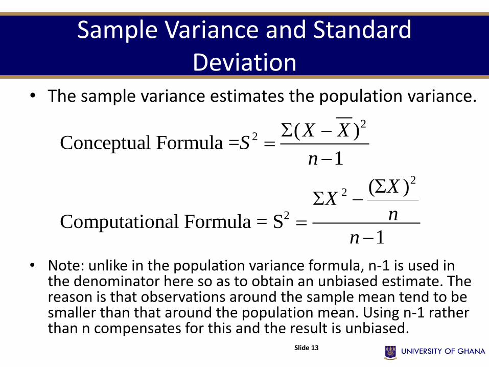
• The sample variance estimates the population variance.

• Note: unlike in the population variance formula, n-1 is used in the denominator here so as to obtain an unbiased estimate. The reason is that observations around the sample mean tend to be smaller than that around the population mean. Using n-1 rather than n compensates for this and the result is unbiased.

Slide 13

22

22

2

( )Conceptual Formula =

1

( )

Computational Formula = S1

X XS

n

XX

n

n


• A sample of five hourly wages for various jobs on campus is: 7, 5, 11, 8, 6. Find the variance.

• The sample standard deviation (s) is the square root of the sample variance.

• So the sample standard deviation is

Slide 14

2 2 2 2 22

7 5 11 8 6 377.4

5 5

( ) [(7 7.4) (5 7.4) (11 7.4) (8 7.4) (6 7.4) ]

1 5 1

21.15.3

4

XX

n

X Xs

n

5.3 2.3s

MEASURES OF DISPERSION FOR GROUPED DATA

Topic Two


• The formula for the sample variance for grouped data used as an estimator of the population variance is:

• Or

• where f is class frequency and X is class midpoint.

Slide 16

2

2

1

f X Xs

n

22

2

( )

1

fXfX

nsn


• The sample variance gives an unbiased estimate of the population variance.

• The sample standard deviation is obtained by taking the square root of the sample variance.

Slide 17

Slide 18

OTHER MEASURES OF DISPERSION

Topic Three

Coefficient of Variation

• The coefficient of variation is the ratio of the standard deviation to the arithmetic mean, expressed as a percentage:

• It is used compare the relative dispersion in distributions measured in different units (or measured in same units but are wide apart (for example, the incomes of top executives and unskilled workers)).

• The relative dispersion measure thus becomes unitless and enables direct comparison of the relative variation in the two distributions.

Slide 19

)100(X

sCV

Coefficient of Variation

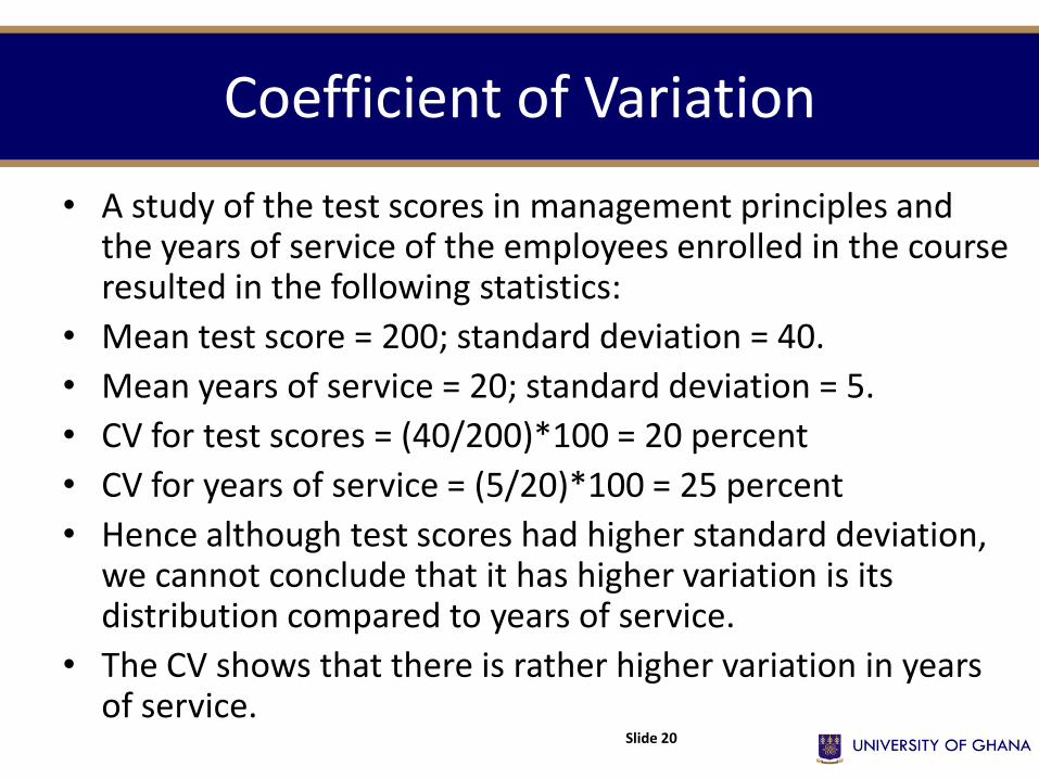
• A study of the test scores in management principles and the years of service of the employees enrolled in the course resulted in the following statistics:

• Mean test score = 200; standard deviation = 40.

• Mean years of service = 20; standard deviation = 5.

• CV for test scores = (40/200)*100 = 20 percent

• CV for years of service = (5/20)*100 = 25 percent

• Hence although test scores had higher standard deviation, we cannot conclude that it has higher variation is its distribution compared to years of service.

• The CV shows that there is rather higher variation in years of service.

Slide 20

Percentiles, Quartiles and Deciles

• The median divides the data arranged in ascending

order into two equal halves; it is also the value such

that 50% of observations are below and 50% above.

• Percentiles divide a set of observations into 100

equal parts.

• A percentile is the value such that P% of

observations are below and (100-P)% are above this

value.

Slide 21


• For example, the 10th percentile is the value such that 10% of observations are below this value and 90% are above.

• We saw earlier that we can locate the position of the median using the formula; (n+1)/2

• We could write it generally as (n+1)(P/100) and since in this case P = 50, we get (n+1)(50/100) = (n+1)/2.

Slide 22


• Thus to determine a given percentile in a distribution, we first locate its position using the formula

• Consider the following data: 37, 59, 71, 75, 78, 78, 81, 86, 88, 92, 95, 96

• Assuming we want the 25th percentile, then Lp= (12+1)(25/100)=3.25 • Hence the 25th percentile is a quarter of the distance

between the 3rd and 4th observations, which gives us 71 + 0.25 (75-71) = 71 + 0.25(4) = 72

Slide 23

Lp np

( )1100


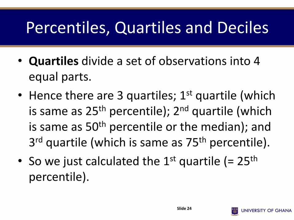
• Quartiles divide a set of observations into 4 equal parts.

• Hence there are 3 quartiles; 1st quartile (which is same as 25th percentile); 2nd quartile (which is same as 50th percentile or the median); and 3rd quartile (which is same as 75th percentile).

• So we just calculated the 1st quartile (= 25th percentile).

Slide 24


• Similarly, deciles divide a set of observations into 10 equal parts; so there are 9 deciles.

• The 1st decile is the same as the 10th percentile and the 5th decile is the same as the 50th percentile or the median.

• In the same vein, each data set has 99 percentiles, thus dividing the data set into 100 equal parts.

• The percentile formula described on the previous slide is applied in calculating quartiles as well as deciles.

Slide 25


• Assuming we wish to calculate the 90th, then

Lp = (12+1)(90/100) = 11.7

• So the 90th percentile is 70% of the distance between the 11th and 12th observations, which gives

95 + 0.7(96-95) = 95.7

Slide 26


• The First Quartile is the value corresponding to the point below which 25% of the observations lie in an ordered data set.

• For grouped data the formula below is applied.

– where L=lower limit of the class containing Q1, CF= cumulative

frequency preceding class containing Q1, f= frequency of class containing Q1, i= size of class containing Q1.

Slide 27

Q L

nCF

fi1

4

( )


• The Third Quartile is the value corresponding to the point below which 75% of the observations lie in an ordered data set:

• The formula is:

– where L=lower limit of the class containing Q3, CF= cumulative frequency preceding class containing Q3, f= frequency of class containing Q3, i= size of class containing Q3.

Slide 28

Q L

nCF

fi3

3

4

( )


• In general, the percentile for grouped data is calculated using the formula:

• where p=percentile we want to calculate, n=number of observations, L=lower limit of the class containing the percentile, CF= cumulative frequency preceding class containing the percentile, f= frequency of class containing the percentile, i= size of class containing the percentile.

Slide 29

)(100 if

CFpn

LP

Inter-quartile and Percentile Ranges

• The Inter-quartile range is the distance between the third quartile Q3 and the first quartile Q1.

• Inter-quartile range = third quartile - first quartile = Q3 - Q1

• The percentile range is the distance between two stated percentiles.

• The 10-to-90 percentile range is the distance between the 10th and 90th percentiles.

Slide 30

Skewness

• Skewness is the measure of the lack of symmetry of a distribution.

• A symmetrical frequency curve is one for which the right half of the curve is the mirror image of the left half.

• If one or more observations of a distribution are extremely large, the mean becomes greater than the median or mode, and the distribution is said to be positively (right) skewed.

Slide 31

Skewness

• Conversely, if one or more extremely small values are present in the data, the mean becomes smaller than the median or mode, and the distribution is said to be negatively (left) skewed.

• The coefficient of skewness is computed from the following formula: Sk = 3(Mean - Median) / (Standard deviation)

Slide 32

Symmetric Distribution

• zero skewness mode = median = mean

3-26

Right Skewed Distribution

• positively skewed: Mean and Median are to

• the right of the Mode.

• Mode<Median<Mean

3-27

Left Skewed Distribution

• Negatively Skewed: Mean and Median are to the left of the Mode.

• Mean<Median<Mode

3-28

Skewness

• Example - The length of stay on the cancer floor of Korle Bu Hospital were organized into a frequency distribution. The mean length of stay is 28 days, the median 25 days and the modal length is 23 days. The standard deviation was computed to be 4.2 days. Is the distribution symmetrical, positively skewed or negatively skewed? Calculate the coefficient of skewness and interpret it.

Slide 36

Skewness

• The distribution is positively skewed because the mean is the largest of the three measures of central tendency.

• Sk = 3(Mean - Median) / (Standard deviation)

• Sk = 3(28 – 25)/4.2 = 2.14

• The coefficient of skewness generally lies between -3 and +3.

• The coefficient of 2.14 indicates a substantial amount of skewness, and shows that a few cancer patients are staying in the hospital for a long time, causing the mean to be larger than the median or mode.

Slide 37

References

• Michael Barrow, “Statistics for Economics, Accounting and Business Studies”, 4th Edition, Pearson

• R.D. Mason , D.A. Lind, and W.G. Marchal, “Statistical Techniques in Business and Economics”, 10th Edition, McGraw-Hill

econ 214 elements of statistics for economists of education school of continuing and distance...

Documents