econ 325: introduction to empirical economics...0.60 0.70 0.80 0.90 0 1 2 3 4 5 6 7 0.9048 0.0905...
TRANSCRIPT
Lecture 3
Discrete Random Variables and Probability Distributions
Econ 325: Introduction to Empirical Economics
Copyright © 2010 Pearson Education, Inc. Publishing as Prentice Hall Ch. 4-1

Introduction to Probability Distributions
n Random Variablen Represents a possible numerical value from
a random experimentRandom Variables
Discrete Random Variable
ContinuousRandom Variable
Ch. 4 Ch. 5
Copyright © 2010 Pearson Education, Inc. Publishing as Prentice Hall Ch. 4-2
4.1

Discrete Random Variablesn Can only take on a countable number of values
Examples:
n Roll a die twiceLet X be the number of times 4 comes up (then X could be 0, 1, or 2 times)
n Toss a coin 3 times. Let X be the number of heads(then X = 0, 1, 2, or 3)
Copyright © 2010 Pearson Education, Inc. Publishing as Prentice Hall Ch. 4-3
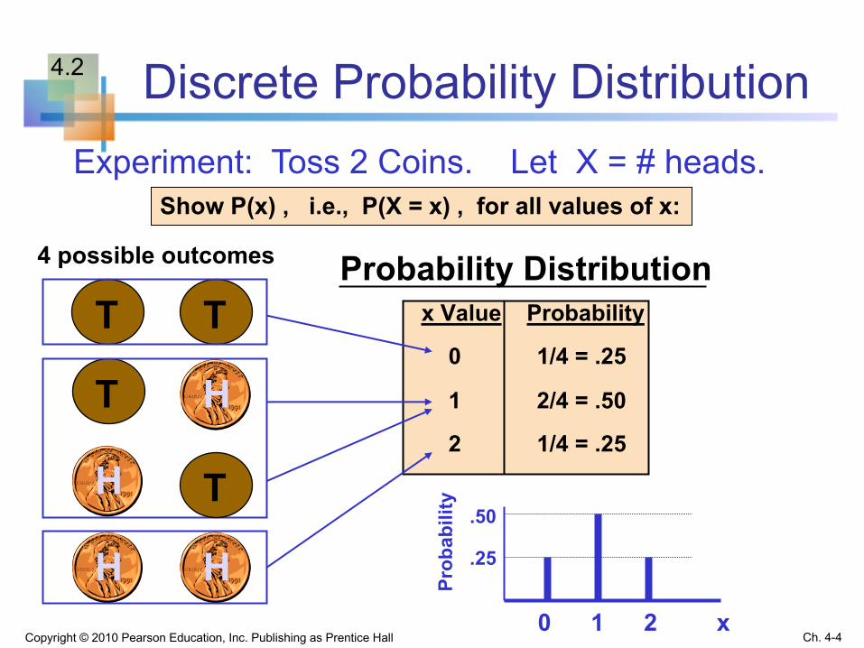
Discrete Probability Distribution
x Value Probability
0 1/4 = .25
1 2/4 = .50
2 1/4 = .25
Experiment: Toss 2 Coins. Let X = # heads.
T
T4 possible outcomes
T
T
H
H
H H
Probability Distribution
0 1 2 x
.50
.25
Prob
abili
ty
Show P(x) , i.e., P(X = x) , for all values of x:
Copyright © 2010 Pearson Education, Inc. Publishing as Prentice Hall Ch. 4-4
4.2

Random variable
n S = {TT, TH, HT, TH}
n Define a function X(s) by
X({TT})=0, X({TH})=1, X({HT})=1, X({HH})=2
n P(X=0) = P({TT}) = 1/4
n P(X=1) = P ({TH,HT}) = 1/2
Ch. 4-5Copyright © 2010 Pearson Education, Inc. Publishing as Prentice Hall

Definition: Random variable
n A random variable X is a function which maps the outcome of an experiment 𝑠 to the real number 𝑥.
𝑋: 𝑆 → 𝑡ℎ𝑒 𝑠𝑝𝑎𝑐𝑒 𝑜𝑓 𝑋n The space of X is given by
𝑆𝑋 = {𝑥: 𝑋 𝑠 = 𝑥, 𝑠 ∈ 𝑆}
Ch. 4-6Copyright © 2010 Pearson Education, Inc. Publishing as Prentice Hall

Discrete Probability Distribution
n The space of X = {0,1,2}.n Define a set A = {0,1} in the space of X. Then,
n Notation: Uppercase ``X’’ represents a random variable and lowercase ``x’’ represents some constant (e.g., realized value).
Ch. 4-7Copyright © 2010 Pearson Education, Inc. Publishing as Prentice Hall
åÎ
=+====ÎAx
1)P(X0)P(X x)P(X A)P(X

Definition: Probability mass function
Copyright © 2010 Pearson Education, Inc. Publishing as Prentice Hall Ch. 4-8
4.3
The probability mass function (pmf) of a discrete random variable X is a function that satisfies the following properties:
1). 𝟎 ≤ 𝐟𝑋 𝒙 ≤ 𝟏2). ∑𝒙∈:; 𝐟𝑋 𝒙 = 13). 𝑷 𝑿 ∈ 𝑨 = ∑𝒙∈𝑨 𝐟𝑋 𝒙

Probability mass function
Ch. 4-9Copyright © 2010 Pearson Education, Inc. Publishing as Prentice Hall
x)P(X)(f X ==x

Cumulative Distribution Function
n The cumulative distribution function, denotedF(x0), is a function defined by the probability of X being less than or equal to x0
å£
=£=0xxX00 (x)f)xP(X)F(x
Copyright © 2010 Pearson Education, Inc. Publishing as Prentice Hall Ch. 4-10

Question
n Define X = # of heads when you toss 2 coins.
n What is the probability mass function and the cumulative distribution function of X?
Ch. 4-11Copyright © 2010 Pearson Education, Inc. Publishing as Prentice Hall
Question
n Define X = a number you get from rolling a die.
n What is the probability mass function and the cumulative distribution function of X?
Ch. 4-12Copyright © 2010 Pearson Education, Inc. Publishing as Prentice Hall
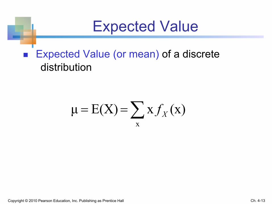
Expected Value
n Expected Value (or mean) of a discretedistribution
å==x
(x)x E(X) μ Xf
Copyright © 2010 Pearson Education, Inc. Publishing as Prentice Hall Ch. 4-13

Example
n What is the expected value when you roll a die once?
n 𝒇𝑿 𝒊 = 𝐏 𝑿 = 𝒊 = 𝟏𝟔
for 𝒊 = 𝟏, 𝟐, … , 𝟔
n 𝑬 𝑿 = ∑𝒊F𝟏𝟔 𝒊× 𝟏𝟔= 𝟑. 𝟓
Ch. 4-14Copyright © 2010 Pearson Education, Inc. Publishing as Prentice Hall

Clicker Question 3-1
Define X = # of heads when you toss 2 coins.What is the expected value of X?
A). 0.5B). 1C). 1.5
Ch. 4-15Copyright © 2010 Pearson Education, Inc. Publishing as Prentice Hall
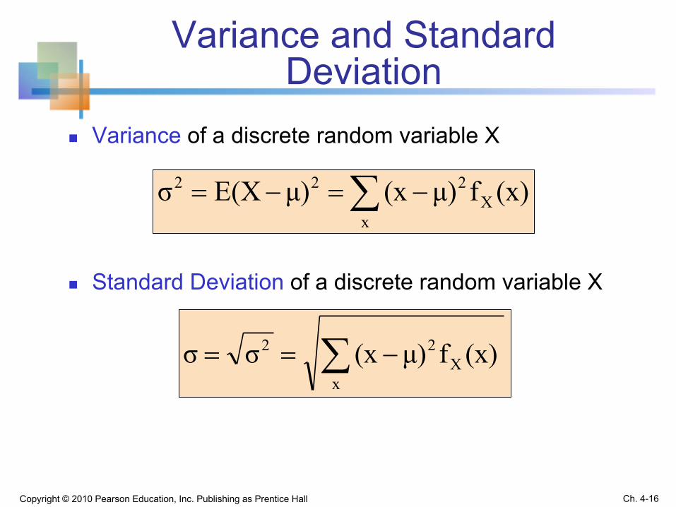
Variance and Standard Deviation
n Variance of a discrete random variable X
n Standard Deviation of a discrete random variable X
å -=-=x
X222 (x)fμ)(xμ)E(Xσ
å -==x
X22 (x)fμ)(xσσ
Copyright © 2010 Pearson Education, Inc. Publishing as Prentice Hall Ch. 4-16

Standard Deviation Example
n Example: Toss 2 coins, X = # heads, compute standard deviation (recall E(x) = 1)
å -=x
X2 (x)fμ)(xσ
.707.50(.25)1)(2(.50)1)(1(.25)1)(0σ 222 ==-+-+-=
Possible number of heads = 0, 1, or 2
Copyright © 2010 Pearson Education, Inc. Publishing as Prentice Hall Ch. 4-17

Clicker Question 3-2
n Toss 1 coin. Let X = 1 if it is head and X=0 if it is tail. What is the variance of this random variable?
A). 1B). 0.5C). 0.25D). 0.1
Ch. 4-18Copyright © 2010 Pearson Education, Inc. Publishing as Prentice Hall

Functions of Random Variables
n If P(x) is the probability function of a discrete random variable X , and g(X) is some function of X , then the expected value of function g is
å=x
X (x)g(x)fE[g(X)]
Copyright © 2010 Pearson Education, Inc. Publishing as Prentice Hall Ch. 4-19

Clicker Question 3-3
n Toss 1 coin. Let X = 1 if it is head and X=0 if it is tail. Consider a function g(X) such that g(1) = 100 and g(0) = 0. What is E[g(X)]?
A). 0B). 100C). 50D). 10
Ch. 4-20Copyright © 2010 Pearson Education, Inc. Publishing as Prentice Hall

Linear Functions of Random Variables
n Let a and b be any constants.
n a)
i.e., if a random variable always takes the value a, it will have mean a and variance 0
n b)
i.e., the expected value of b·X is b·E(X)
0Var(a)andaE(a) ==
E(bX) = bE(X) and Var(bX) = b2Var(X)
Copyright © 2010 Pearson Education, Inc. Publishing as Prentice Hall Ch. 4-21

Linear Functions of Random Variables
n Let random variable X have mean µx and variance σ2x
n Let a and b be any constants. n Let Y = a + bXn Then the mean and variance of Y are
n so that the standard deviation of Y is
E(Y) = E(a + bX) = a + bE(X)
Var(X)bbX)Var(aVar(Y) 2=+=
XY σbσ =
(continued)
Copyright © 2010 Pearson Education, Inc. Publishing as Prentice Hall Ch. 4-22

Bernoulli Distribution
n Consider only two outcomes: “success” or “failure” n Let p denote the probability of successn Let 1 – p be the probability of failure n Define random variable X:
X = 1 if success, X = 0 if failuren Then the Bernoulli probability function is
p1)P(X andp)(10)P(X ==-==
Copyright © 2010 Pearson Education, Inc. Publishing as Prentice Hall Ch. 4-23

Possible Bernoulli Distribution Settings
n A survey responses of ``I will vote for the Liberal Party’’ or ``I will vote for the Conservative Party’’
n A manufacturing plant labels items as either defective or acceptable
n A marketing research firm receives survey responses of “yes I will buy” or “no I will not”
Copyright © 2010 Pearson Education, Inc. Publishing as Prentice Hall Ch. 4-24

Bernoulli DistributionMean and Variance
n The mean is µ = p
n The variance is σ2 = p(1 – p)
µ= E(X) = xx=0,1∑ P(X = x) = (0)(1− p)+ (1)p = p
σ 2 = E[(X−µ)2 ]= (x−µ)2P(X = x)x=0,1∑
= (0− p)2(1− p)+ (1− p)2p = p(1− p)
Copyright © 2010 Pearson Education, Inc. Publishing as Prentice Hall Ch. 4-25

2019 Canadian federal election
Ch. 4-26Copyright © 2010 Pearson Education, Inc. Publishing as Prentice Hall
Canada Poll Tracker: CBC News
338Canada

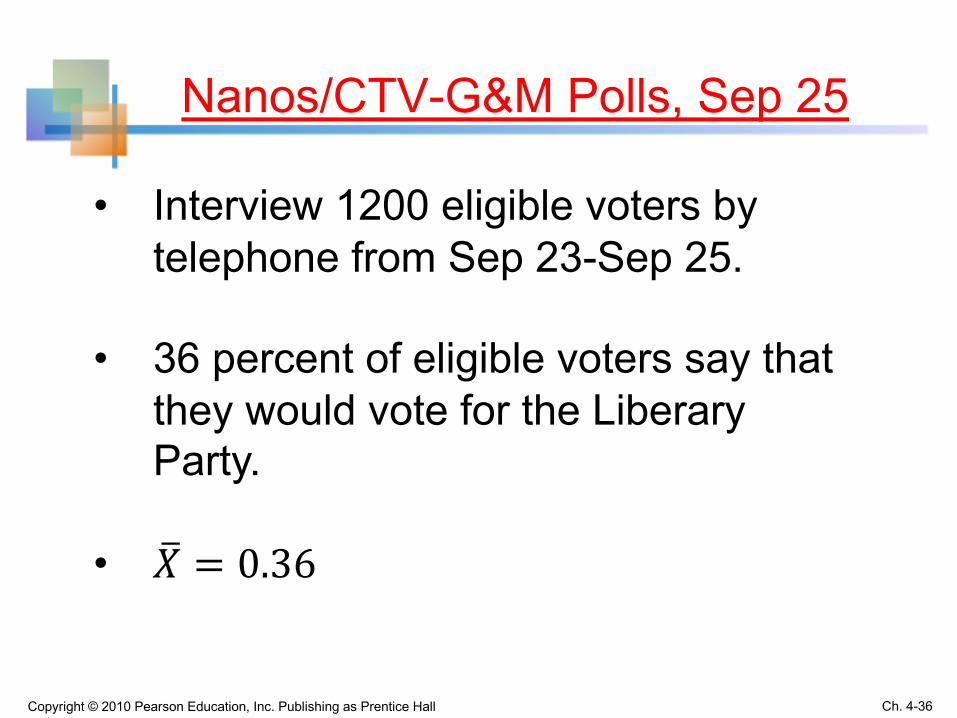
Nanos/CTV-G&M Polls, Sep 25
Ch. 4-27Copyright © 2010 Pearson Education, Inc. Publishing as Prentice Hall
• Interview 1200 eligible voters by telephone from Sep 23-Sep 25.
• Out of 1200, 432 eligible voters say that they would vote for the LiberaryParty.

Question
Ch. 4-28Copyright © 2010 Pearson Education, Inc. Publishing as Prentice Hall
𝑋K = 1 if ``I will vote for the Liberal Party’’𝑝 = 𝑃 𝑋K = 1 = the population fraction of voters who vote for the Liberal Party Let 𝑋N, 𝑋O, and 𝑋P be survey responses from randomly sampled three individuals.What is the probability mass function of 𝑌 = 𝑋N + 𝑋O + 𝑋P?

Question
Ch. 4-29Copyright © 2010 Pearson Education, Inc. Publishing as Prentice Hall
Let 𝑋K for 𝑖 = 1,2, … , 𝑛 are survey responses from randomly sampled n individuals with 𝑃 𝑋K = 1 = 𝑝.
What is the probability mass function of
𝑌 = ∑KFNV 𝑋K ?
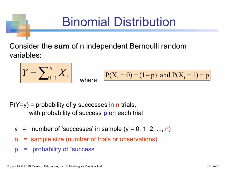
Binomial Distribution
Consider the sum of n independent Bernoulli random variables:
, where
P(Y=y) = probability of y successes in n trials,with probability of success p on each trial
y = number of ‘successes’ in sample (y = 0, 1, 2, ..., n)n = sample size (number of trials or observations)p = probability of “success”
Copyright © 2010 Pearson Education, Inc. Publishing as Prentice Hall Ch. 4-30
p1)P(X and p)(10)P(X ii ==-==å ==
n
i iXY1

Probability mass function of Binomial distribution
P(y) = probability of y successes in n trials,with probability of success p on each trial
y = number of ‘successes’ in sample, (y = 0, 1, 2, ..., n)
n = sample size (number of trials or observations)
p = probability of “success”
P(Y=y)n
y ! n yp (1- p)y n y!
( )!=
--
Copyright © 2010 Pearson Education, Inc. Publishing as Prentice Hall Ch. 4-31

Clicker Question 3-4
Randomly sampled 3 individuals. What is the probability that 2 out of 3 person supports the Liberal party if p=0.4?
(A). 0.4 × (1 − 0.4)O
(B). (1 − 0.4)× (0.4)O
(C). 3×0.4 × (1 − 0.4)O
(D). 3×(1 − 0.4)× (0.4)O
Ch. 4-32Copyright © 2010 Pearson Education, Inc. Publishing as Prentice Hall
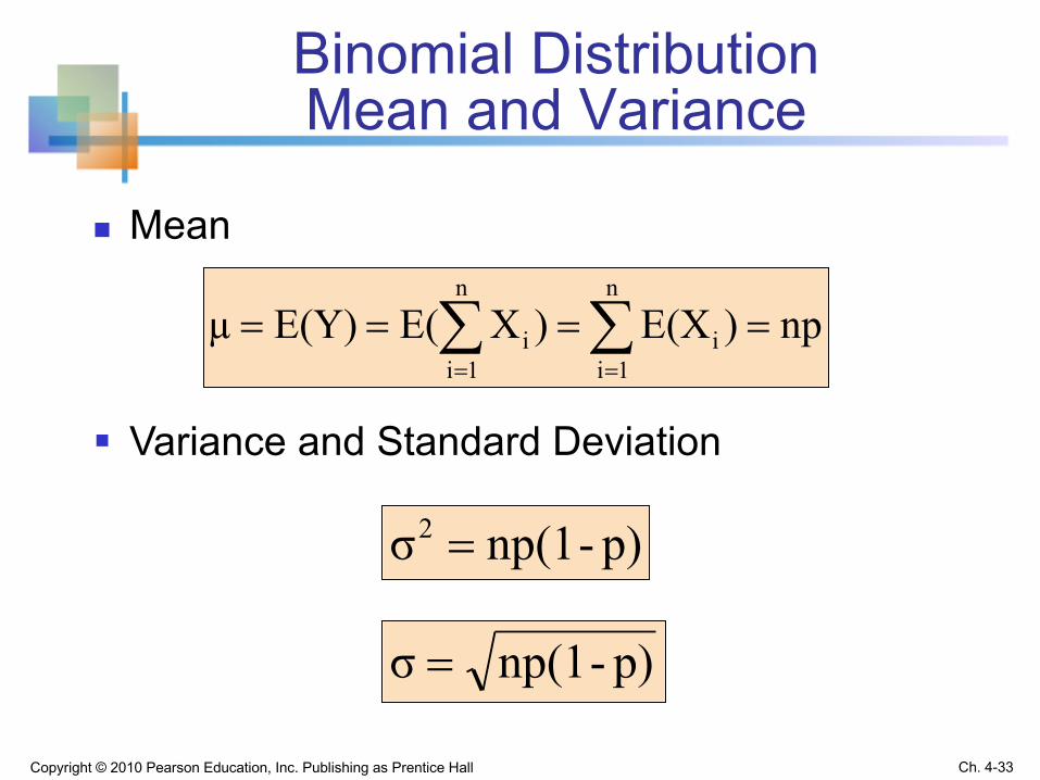
Binomial DistributionMean and Variance
n Mean
§ Variance and Standard Deviation
np)E(X)XE(E(Y)µn
1ii
n
1ii ==== åå
==
p)-np(1σ2 =
p)-np(1σ =
Copyright © 2010 Pearson Education, Inc. Publishing as Prentice Hall Ch. 4-33

Average of n independent Bernoulli random variable
Consider the sample average of n independent Bernoulli random variable:
, with
Then, ]𝑋 is related to Binomial random variable 𝑌 = ∑KFNV 𝑋K as
Copyright © 2010 Pearson Education, Inc. Publishing as Prentice Hall Ch. 4-34
p)(10)P(X and p1)P(X ii -====å ==
n
i iXnX
1
1
Yn
Xn
X n
i i11
1== å =
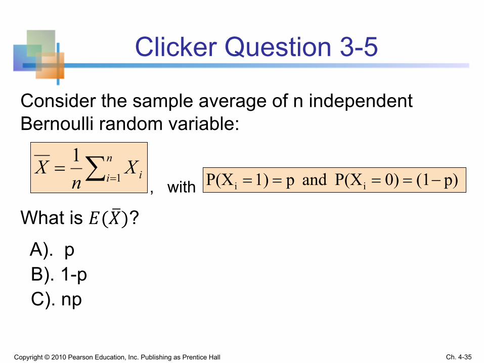
Clicker Question 3-5
Consider the sample average of n independent Bernoulli random variable:
, with
What is 𝐸( ]𝑋)?A). pB). 1-pC). np
Copyright © 2010 Pearson Education, Inc. Publishing as Prentice Hall Ch. 4-35
p)(10)P(X and p1)P(X ii -====å ==
n
i iXnX
1
1
Nanos/CTV-G&M Polls, Sep 25
Ch. 4-36Copyright © 2010 Pearson Education, Inc. Publishing as Prentice Hall
• Interview 1200 eligible voters by telephone from Sep 23-Sep 25.
• 36 percent of eligible voters say that they would vote for the LiberaryParty.
• ]𝑋 = 0.36

Poisson Distribution Function
n The Poisson probability distribution gives the probability of a number of events occurring in a fixed interval of time or space.
n Examples:n The number of telephone calls to 911 in a large city
from 1am to 5am.n The number of delivery trucks to arrive at a central
warehouse in an hour. n The number of customers to arrive at a checkout
aisle in your local grocery store from 2pm to 3pm.
Ch. 4-37Copyright © 2010 Pearson Education, Inc. Publishing as Prentice Hall

Poisson Distribution Function
n Assume an interval is divided into a very large number of ``very short’’ subintervals with equal length h.
1. The number of occurrences in subintervals are independent.
2. The probability of exactly one occurrence in a subinterval of length h is approximately 𝜆h.
3. The probability of two or more occurrences approaches zero as the length h approaches zero.
Ch. 4-38Copyright © 2010 Pearson Education, Inc. Publishing as Prentice Hall

Poisson Distribution Function
Ch. 4-39Copyright © 2010 Pearson Education, Inc. Publishing as Prentice Hall
n The expected number of occurrences per time/space unit is the parameter l (lambda).
( )xeP x
x
ll-
=!
where:P(x) = the probability of x occurrences over one unit of time or spacel = the expected number of occurrences per time/space unit, l > 0
e = base of the natural logarithm system (2.71828...)
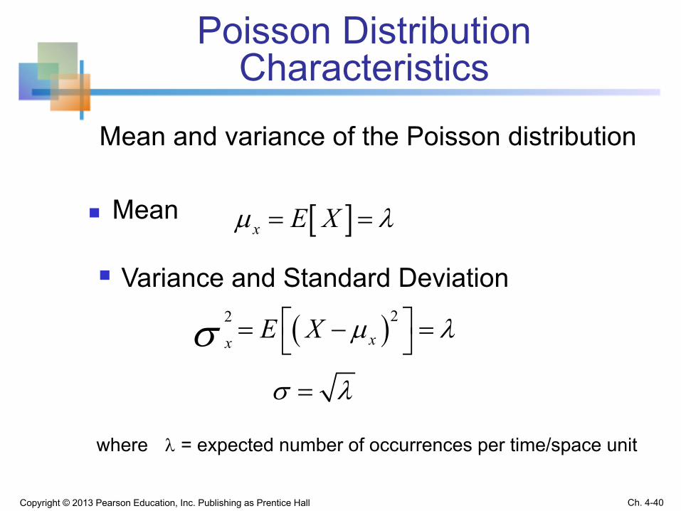
Poisson Distribution Characteristics
n Mean
§ Variance and Standard Deviation
where l = expected number of occurrences per time/space unit
Copyright © 2013 Pearson Education, Inc. Publishing as Prentice Hall Ch. 4-40
Mean and variance of the Poisson distribution
[ ]x E Xµ l= =
( )22xx E X µ ls é ù= - =ë û
s l=
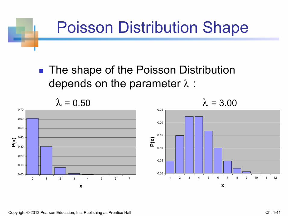
Poisson Distribution Shape
n The shape of the Poisson Distribution depends on the parameter l :
0.00
0.05
0.10
0.15
0.20
0.25
1 2 3 4 5 6 7 8 9 10 11 12
x
P(x)
0.00
0.10
0.20
0.30
0.40
0.50
0.60
0.70
0 1 2 3 4 5 6 7
x
P(x)
l = 0.50 l = 3.00
Copyright © 2013 Pearson Education, Inc. Publishing as Prentice Hall Ch. 4-41

Example
You are the CEO of a grocery store. Customers arrive at checkout counters at an average rate of 1 customer every 2 minutes. Assume that these arrivals are independent over time.
What is the probability that more than two customers arrive within one minute?
In this case, the expected number of customers per minute is 𝜆 = 1/2 = 0.5
Ch. 4-42Copyright © 2010 Pearson Education, Inc. Publishing as Prentice Hall

Using Poisson Tables
X
l
0.10 0.20 0.30 0.40 0.50 0.60 0.70 0.80 0.90
01234567
0.90480.09050.00450.00020.00000.00000.00000.0000
0.81870.16370.01640.00110.00010.00000.00000.0000
0.74080.22220.03330.00330.00030.00000.00000.0000
0.67030.26810.05360.00720.00070.00010.00000.0000
0.60650.30330.07580.01260.00160.00020.00000.0000
0.54880.32930.09880.01980.00300.00040.00000.0000
0.49660.34760.12170.02840.00500.00070.00010.0000
0.44930.35950.14380.03830.00770.00120.00020.0000
0.40660.36590.16470.04940.01110.00200.00030.0000
Example: Find P(X = 2) if l = .50
.07582!(0.50)e
!Xe)2X(P
20.50X
==l
==-l-
Copyright © 2013 Pearson Education, Inc. Publishing as Prentice Hall Ch. 4-43

Graph of Poisson Probabilities
0.00
0.10
0.20
0.30
0.40
0.50
0.60
0.70
0 1 2 3 4 5 6 7
x
P(x)X
l =0.50
01234567
0.60650.30330.07580.01260.00160.00020.00000.0000
P(X = 2) = .0758
Graphically:l = .50
Copyright © 2013 Pearson Education, Inc. Publishing as Prentice Hall Ch. 4-44

Clicker Question 3-6
Customers independently arrive at counters at an average rate of 1 customer every 2 minutes.
What is the probability that more than two customers arrive within one minute?
A). 0.0758B). 0.0886C). 0.6065
Ch. 4-45Copyright © 2010 Pearson Education, Inc. Publishing as Prentice Hall

Poisson and Binomial Distribution
Ch. 4-46Copyright © 2010 Pearson Education, Inc. Publishing as Prentice Hall
n Divide one unit of time into n subintervals, each of which has length of h = 1/n.
n For sufficiently large n, the probability of one occurrence is given by 𝜆h=𝜆/n ⇒ a sequence of n Bernoulli trials.
n The number of occurrences within one unit of time is approximate by the sum of n Bernoulli trials, i.e., Binomial distribution:
𝑃 𝑋 = 𝑥 ≈ V!d! Ved !
fV
d1 − f
V
Ved
→ fghi
d!as n → ∞

Poisson and Binomial Distribution
Ch. 4-47Copyright © 2010 Pearson Education, Inc. Publishing as Prentice Hall
n Set p = 𝜆/n ⇒ 𝜆=np.n Then, we may approximate the binomial distribution by
the Poisson distribution:
𝑃 𝑋 = 𝑥 = V!d! Ved !
pd 1 − p Ved
≈ npghnpd!
if n is large
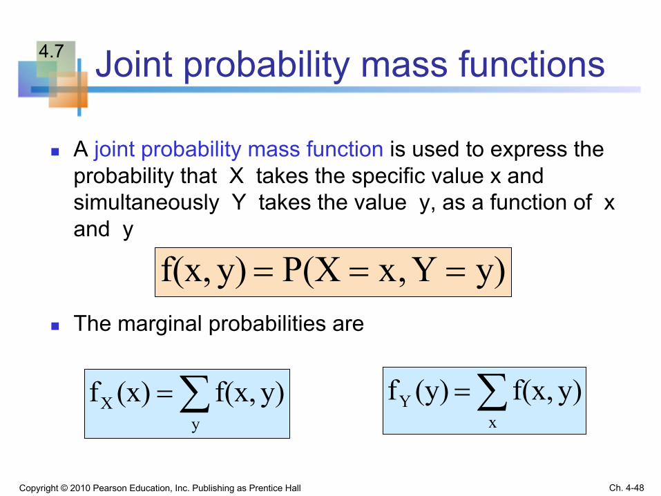
Joint probability mass functions
n A joint probability mass function is used to express the probability that X takes the specific value x and simultaneously Y takes the value y, as a function of x and y
n The marginal probabilities are
y)Y,xP(Xy)f(x, ===
å=y
X y)f(x,(x)f å=x
Y y)f(x,(y)f
Copyright © 2010 Pearson Education, Inc. Publishing as Prentice Hall Ch. 4-48
4.7

Stochastic Independence
n The jointly distributed random variables X and Y are said to be independent if and only if
for all possible pairs of values x and y
n A set of k random variables are independent if and only if
(y)(x)ffy)f(x, YX=
)(xf)(x)f(xf)x,,x,f(x k21k21 21 kXXX !! =
Copyright © 2010 Pearson Education, Inc. Publishing as Prentice Hall Ch. 4-49
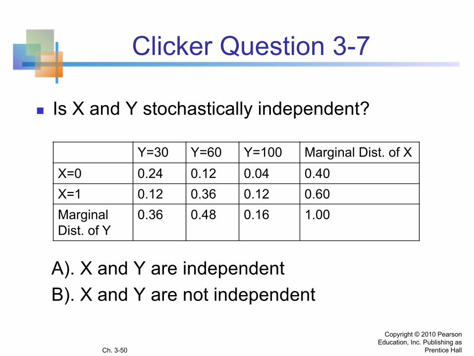
Clicker Question 3-7
n Is X and Y stochastically independent?
A). X and Y are independentB). X and Y are not independent
Copyright © 2010 Pearson Education, Inc. Publishing as
Prentice HallCh. 3-50
Y=30 Y=60 Y=100 Marginal Dist. of XX=0 0.24 0.12 0.04 0.40X=1 0.12 0.36 0.12 0.60Marginal Dist. of Y
0.36 0.48 0.16 1.00

Conditional probability mass functions
n The conditional probability mass function of the random variable Y is define by
n Similarly, the conditional probability mass function of X given Y = y is:
(x)fy)f(x,x)|(yf
XX|Y =
(y)fy)f(x,y)|(xf
YY|X =
Copyright © 2010 Pearson Education, Inc. Publishing as Prentice Hall Ch. 4-51
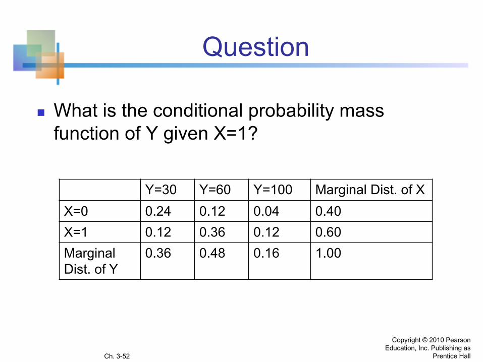
Question
n What is the conditional probability mass function of Y given X=1?
Copyright © 2010 Pearson Education, Inc. Publishing as
Prentice HallCh. 3-52
Y=30 Y=60 Y=100 Marginal Dist. of XX=0 0.24 0.12 0.04 0.40X=1 0.12 0.36 0.12 0.60Marginal Dist. of Y
0.36 0.48 0.16 1.00
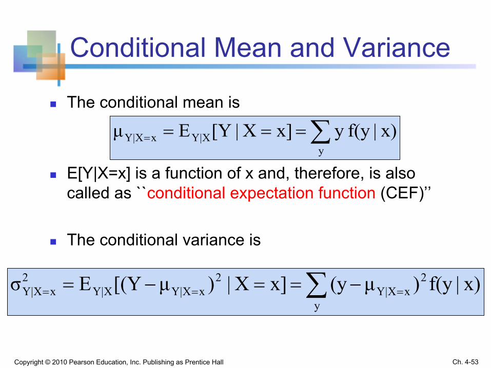
Conditional Mean and Variance
Ch. 4-53Copyright © 2010 Pearson Education, Inc. Publishing as Prentice Hall
n The conditional mean is
n E[Y|X=x] is a function of x and, therefore, is also called as ``conditional expectation function (CEF)’’
n The conditional variance is
x)|f(yy x]X|[YEμy
X|YxX|Y å====
å === -==-=y
2xX|Y
2xX|YX|Y
2xX|Y x)|f(y)μ(yx]X|)μ[(YEσ
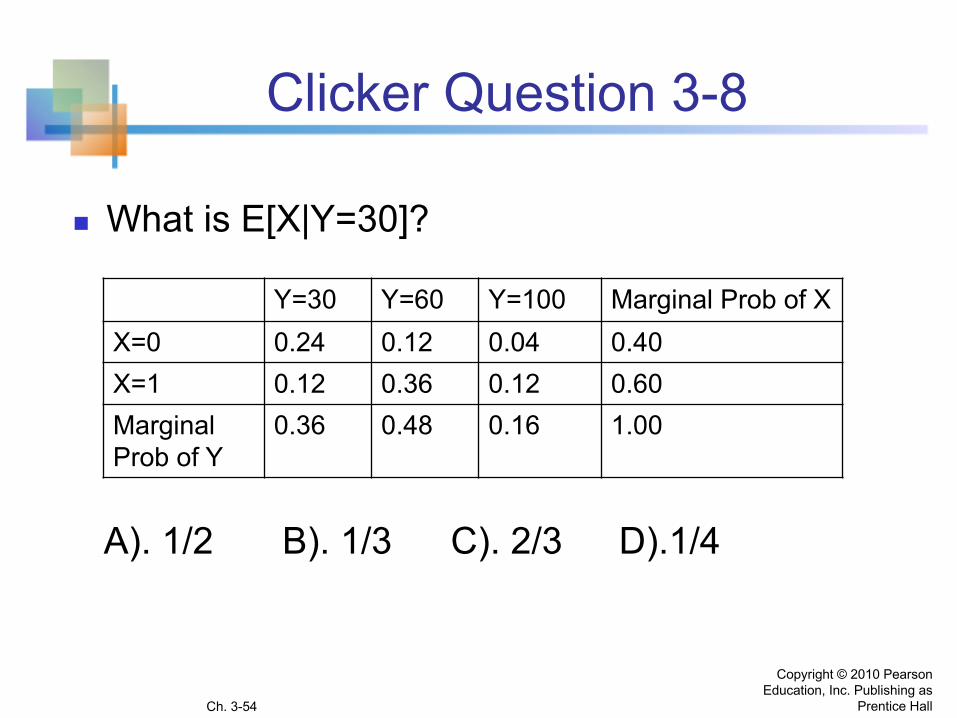
Clicker Question 3-8
n What is E[X|Y=30]?
A). 1/2 B). 1/3 C). 2/3 D).1/4
Copyright © 2010 Pearson Education, Inc. Publishing as
Prentice HallCh. 3-54
Y=30 Y=60 Y=100 Marginal Prob of XX=0 0.24 0.12 0.04 0.40X=1 0.12 0.36 0.12 0.60Marginal Prob of Y
0.36 0.48 0.16 1.00

Clicker Question 3-9
n What is Var[X|Y=30]?
A). 1/9 B). 1/3 C). 2/9 D). 2/27
Copyright © 2010 Pearson Education, Inc. Publishing as
Prentice HallCh. 3-55
Y=30 Y=60 Y=100 Marginal Prob of XX=0 0.24 0.12 0.04 0.40X=1 0.12 0.36 0.12 0.60Marginal Prob of Y
0.36 0.48 0.16 1.00

𝐸l|;[𝑌|𝑋] as a random variable
n Viewing X as a random variable, 𝐸l|;[𝑌|𝑋] is a random variable because the value of 𝐸l|;[𝑌|𝑋]depends on a realization of X.
n The Law of Iterated Expectations:
𝐸;[𝐸l|;[𝑌|𝑋]] = 𝐸l[𝑌]
Ch. 4-56Copyright © 2010 Pearson Education, Inc. Publishing as Prentice Hall

Covariance
n Let X and Y be discrete random variables with means μX and μY
n The expected value of (X - μX)(Y - μY) is called the covariance between X and Y
n For discrete random variables
åå --=--=x y
YXYX y))f(x,μ)(yμ(x)]μ)(YμE[(XY)Cov(X,
Copyright © 2010 Pearson Education, Inc. Publishing as Prentice Hall Ch. 4-57

Correlation
n The correlation between X and Y is:
n ρ = 0 : no linear relationship between X and Yn ρ > 0 : positive linear relationship between X and Y
n when X is high (low) then Y is likely to be high (low)n ρ = +1 : perfect positive linear dependency
n ρ < 0 : negative linear relationship between X and Yn when X is high (low) then Y is likely to be low (high)n ρ = -1 : perfect negative linear dependency
YXσσY)Cov(X,Y)Corr(X,ρ ==
Copyright © 2010 Pearson Education, Inc. Publishing as Prentice Hall Ch. 4-58

Uncorrelatedness, Mean Independence, Stochastic Independence
n X and Y are said to be uncorrelated when Cov(X,Y)=0 or 𝜌 = 0.
n X is said to be mean independent of Y when 𝐸;|l 𝑋 𝑌 = 𝐸;[𝑋].
n X and Y are said to be stochastically independent when 𝑓 𝑥, 𝑦 = 𝑓; 𝑥 𝑓l 𝑦 .
Copyright © 2010 Pearson Education, Inc. Publishing as Prentice Hall Ch. 4-59

Uncorrelatedness, Mean Independence, Stochastic Independence
Stochastic Independence 𝑓 𝑥, 𝑦 = 𝑓; 𝑥 𝑓l 𝑦
⇓Mean Independence
𝐸;|l 𝑋 𝑌 = 𝐸;[𝑋] or 𝐸l|; 𝑌 𝑋 = 𝐸l[𝑌]
⇓Uncorrelatedness
Cov(X,Y)=0Copyright © 2010 Pearson Education, Inc. Publishing as Prentice Hall Ch. 4-60

Clicker Question 3-10
n Suppose X and Y are stochastically independent. Then,
A). the conditional mean of X given Y=y is the same as the unconditional mean of X.
B). the conditional mean of X given Y=y may not be the same as the unconditional mean of X.
Ch. 4-61Copyright © 2010 Pearson Education, Inc. Publishing as Prentice Hall

𝑉𝑎𝑟 𝑎𝑋 + 𝑏𝑌
n For any constant a and b and any two random variables X and Y,
𝑉𝑎𝑟 𝑎𝑋 + 𝑏𝑌 = 𝑎O𝑉𝑎𝑟 𝑋 + 𝑏O𝑉𝑎𝑟 𝑌+2𝑎𝑏 𝐶𝑜𝑣 𝑋, 𝑌
Ch. 4-62Copyright © 2010 Pearson Education, Inc. Publishing as Prentice Hall

Clicker Question 3-10
n Which of the following is true.
A). 𝑉𝑎𝑟 𝑎𝑋 + 𝑏𝑌 = 𝑎O𝑉𝑎𝑟 𝑋 + 𝑏O𝑉𝑎𝑟 𝑌+2𝑎𝑏 𝐶𝑜𝑟𝑟 𝑋, 𝑌
B). 𝑉𝑎𝑟 𝑎𝑋 + 𝑏𝑌 = 𝑎O𝑉𝑎𝑟 𝑋 + 𝑏O𝑉𝑎𝑟 𝑌+2𝑎𝑏𝜎;𝜎l𝐶𝑜𝑟𝑟 𝑋, 𝑌
C). 𝑉𝑎𝑟 𝑎𝑋 + 𝑏𝑌 = 𝑎O𝑉𝑎𝑟 𝑋 + 𝑏O𝑉𝑎𝑟 𝑌+2𝑎𝑏𝐶𝑜𝑟𝑟 𝑋, 𝑌 /𝜎;𝜎l
Ch. 4-63Copyright © 2010 Pearson Education, Inc. Publishing as Prentice Hall
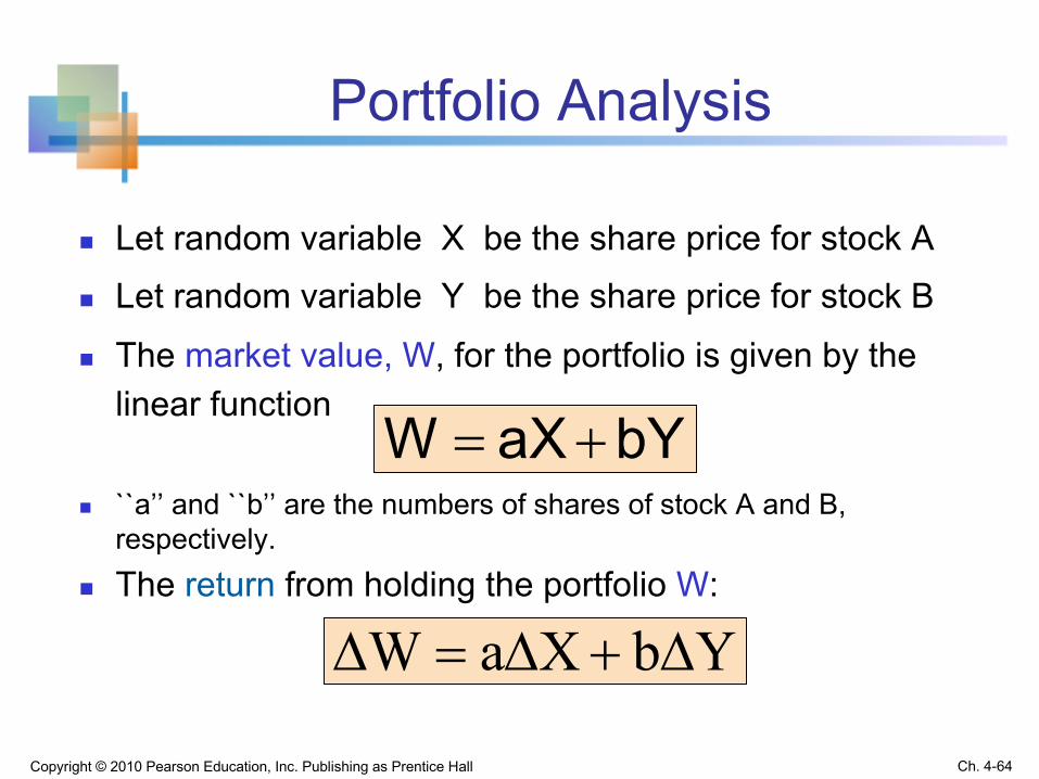
Portfolio Analysis
n Let random variable X be the share price for stock A n Let random variable Y be the share price for stock B
n The market value, W, for the portfolio is given by the linear function
n ``a’’ and ``b’’ are the numbers of shares of stock A and B, respectively.
n The return from holding the portfolio W:
bYaXW +=
Copyright © 2010 Pearson Education, Inc. Publishing as Prentice Hall Ch. 4-64
YbXaW D+D=D

Portfolio Analysis
n The mean value for ∆W is
n The variance for ∆W is
or using the correlation formula
(continued)
Y]bE[X]aE[Y]bXE[aW]E[
D+D=D+D=D
Y),2abCov(σbσaσ 2Y
22X
22W DD++= DDD X
YX2Y
22X
22W σY)σX,2abCorr(σbσaσ DDDDD DD++=
Copyright © 2010 Pearson Education, Inc. Publishing as Prentice Hall Ch. 4-65

Asset Class Correlation Matrix
Ch. 4-66Copyright © 2010 Pearson Education, Inc. Publishing as Prentice Hall

Example: Investment Returns
Return per $100 for two types of investments
P(∆X,∆Y) Economic condition Bond Fund X Aggressive Fund Y
0.2 Recession + $ 7 - $20
0.5 Stable Economy + 4 + 6
0.3 Expanding Economy + 2 + 35
Investment
E(∆X) = (7)(.2) +(4)(.5) + (2)(.3) = 4
E(∆Y) = (-20)(.2) +(6)(.5) + (35)(.3) = 9.5
Copyright © 2010 Pearson Education, Inc. Publishing as Prentice Hall Ch. 4-67

Computing the Standard Deviation for Investment Returns
P(∆X,∆Y) Economic condition Bond Fund X Aggressive Fund Y
0.2 Recession + $ 7 - $20
0.5 Stable Economy + 4 + 6
0.3 Expanding Economy + 2 + 35
Investment
731.3
(0.3)4)(2(0.5)4)(4(0.2)4)(7X)Var( 222X
»=
-+-+-=D=Ds
19.3725.375
(0.3)9.5)(35(0.5)9.5)(6(0.2)9.5)(-20Y)Var( 222Y
»=
-+-+-=D=Ds
Copyright © 2010 Pearson Education, Inc. Publishing as Prentice Hall Ch. 4-68

Covariance for Investment Returns
P(∆X,∆Y) Economic condition Bond Fund X Aggressive Fund Y
0.2 Recession + $ 7 - $20
0.5 Stable Economy + 4 + 6
0.3 Expanding Economy + 2 + 35
Investment
-339.5)(.3)4)(35(2
9.5)(.5)4)(6(49.5)(.2)20-4)((7Y)X,Cov(YX
=--+
--+--=DD=DDs
Copyright © 2010 Pearson Education, Inc. Publishing as Prentice Hall Ch. 4-69

Portfolio Example
Investment X: E(∆X)= 4 σ∆X = 1.73Investment Y: E(∆Y)= 9.5 σ∆Y = 19.32
σ∆X∆Y = -33
Suppose 40% of the portfolio (W) is in Investment X and 60% is in Investment Y:
𝑉𝑎𝑟 ∆𝑊 = .4(1.73)O+ .6(19.32)O+2 .4 (.6)(−33) = 14.47
The portfolio return and portfolio variability are between the values for investments X and Y considered individually
3.7)5.9()6(.)4(4.W)E( =+=D
Copyright © 2010 Pearson Education, Inc. Publishing as Prentice Hall Ch. 4-70

Interpreting the Results for Investment Returns
n The aggressive fund has a higher expected return, but much more risk
E(∆Y)= 9.5 > E(∆X) = 4but
σ∆Y = 19.32 > σ∆X = 1.73
n The Covariance of -33 indicates that the two investments are negatively related and will vary in the opposite direction
Copyright © 2010 Pearson Education, Inc. Publishing as Prentice Hall Ch. 4-71