Econometric analysis of games with multiple equilibria

Áureo de Paula

The Institute for Fiscal Studies Department of Economics, UCL

cemmap working paper CWP29/12

Econometric Analysis of Games with Multiple Equilibria

⇤

Aureo de Paula†

University College London, CeMMAP and IFS

This Version: September, 2012

Abstract

This article reviews the recent literature on the econometric analysis of games where

multiple solutions are possible. Multiplicity does not necessarily preclude the estima-

tion of a particular model (and in certain cases even improves its identification), but

ignoring it can lead to misspecifications. The survey starts with a general characteriza-

tion of structural models that highlights how multiplicity a↵ects the classical paradigm.

Because the information structure is an important guide to identification and estima-

tion strategies, I discuss games of complete and incomplete information separately.

Whereas many of the techniques discussed in the article can be transported across dif-

ferent information environments, some of them are specific to particular models. I also

survey models of social interactions in a di↵erent section. I close with a brief discussion

of post-estimation issues and research prospects.

KEYWORDS: Identification, multiplicity, games, social interactions.

⇤I would like to thank Tim Halliday, Chris Julliard, Elie Tamer and Matthew Weinberg for discussions

and suggestions. I am very grateful to the Editor, Chuck Manski, who provided detailed comments which

markedly improved this survey. Financial support from the Economic and Social Research Council through

the ESRC Centre for Microdata Methods and Practice grant RES-589-28-0001 and the National Science

Foundation through grant award number SES 1123990 is gratefully acknowledged. When citing this paper,

please use the following: de Paula, A. 2013. Econometric Analysis of Games with Multiple Equilibria. Annu.

Rev. Econ. 5: Submitted. Doi: 10.1146/annurev-economics-081612-185944.†University College London, CeMMAP and IFS, London, UK. E-mail: apaula@ucl.ac.uk

1

1 Introduction

In this article I review the recent literature on the econometric analysis of games where

multiple solutions are possible. Equilibrium models are a defining ingredient of Economics.

Game theoretic models in particular have occupied a prominent role in various subfields of

the discipline for many decades. When taking these models to data, a sample of games repre-

sented by markets, neighborhoods, or economies, is endowed with an interdependent payo↵

structure that depends on observable and unobservable variables (to the econometrician and

potentially to the players) and participants choose actions. One pervasive feature in many

of these models is the existence of multiple solutions for various payo↵ configurations, and

this is an aspect that carries over to estimable versions of such systems.

Whereas the existence of more than one solution for a given realization of the pay-

o↵ structure does not preclude the estimation of a particular model (and in certain cases

even improves their identification), ignoring its possible occurrence opens the door to poten-

tially severe misspecifications and non-robustness in the analysis of substantive questions.

Fortunately a lot has been learnt in the recent past about the econometric properties of

such models. The tools available benefit from advances in identification analysis, estimation

techniques, and computational capabilities. I cover some of these in the ensuing pages.

Given space limitations, the survey is by no means exhaustive. I nevertheless try to

cover some of the main developments thus far. Because most of the literature has so far

concentrated on parametric models, this is also my focus here. As in many other contexts,

which parametric and functional restrictions are imposed deserves careful deliberation and

some of the parametric and functional restrictions in the models I present can be relaxed

(e.g., the linearity of the parametric payo↵ function and the distributional assumptions in

Theorem 2 of Tamer (2003) or the analysis of social interactions models in Brock and Durlauf

(2007)). Once point or partial identification is established, estimation typically proceeds by

applying well understood methods such as Maximum Likelihood and Method of Moments

(many times with the assistance of simulations) in the case of point-identified models, or

by carrying out recently developed methods for partially identified models. A thorough

2

discussion of partially identified models would require much more space and I leave that for

other surveys covering those methods in more generality and detail (see, e.g., Tamer (2010)).

I nevertheless do discuss estimation and computation aspects that are somewhat peculiar to

the environments described in this survey at various points.

In all the games analyzed here, given a set of payo↵s for the economic agents involved,

a solution concept defines the (possibly multiple) outcomes that are consistent with the eco-

nomic environment. The solution concepts I use below essentially consist of mutual best

responses (plus consistent beliefs when information is asymmetrically available) and I refer

to those as “equilibria” or “solutions” indiscriminately (hopefully without much confusion

to the reader). In the following sections, the solution concepts are Nash equilibrium for com-

plete information games, Bayes-Nash or Markov Perfect equilibrium for games of incomplete

information, and rational expectations equilibrium as defined in the social interactions lit-

erature for those types of models. Whereas these are commonly assumed solution concepts,

others exist. Aradillas-Lopez and Tamer (2008) for example consider rationalizable strate-

gies and network formation games rely on pairwise stability or similar concepts. Multiplicity

is often an issue for these alternative definitions and many of the ideas discussed below (e.g.,

bounds) can be used when those concepts are adopted instead.

One important ingredient guiding identification and estimation strategies in these

models is the information environment of a game. Whether a game is one of complete or

incomplete (i.e., private) information may a↵ect the econometric analysis in a substantive

manner. Many of the techniques discussed below can be transported across these di↵erent

information environments, but some of them are specific to particular models. In the next

sections I discuss identification and estimation in games of complete and incomplete infor-

mation separately. I also separately survey models of social interactions, where multiplicity

occur as well. For certain specifications (though not always), these models coincide with

games of incomplete information and the discussion of that class of games carries forward.

Because the number of players in a given economy is typically large in this class of models

though, additional estimation strategies handling multiplicity may be employed. I end the

article with a discussion of post-estimation issues and research prospects.

3

2 Preliminary Foundations

Following early analyses of the problem such as Jovanovic (1989), I start by casting my

discussion in terms of the perspective adopted by Koopmans and co-workers in the mid-

20th century. I do so because it makes it apparent how multiplicity interferes with usual

econometric methodologies and lays many of the models on a common ground, making it

easier to identify discrepancies and commonalities across models. Koopmans and colleagues

recognized that the analysis of economic phenomena often requires that we go beyond the

mere statistical description of the observable probability distributions of interest and pursue

primitive parameters, or policy invariant features, of an economic model. In their own words,

[i]n many fields the objective of the investigator’s inquisitiveness is not just a

“population” in the sense of a distribution of observable variables, but a physical

structure projected behind this distribution, by which the latter is thought to

be generated. (. . . ) [T]he structure concept is based on the investigator’s ideas

as to the “explanation” or “formation” of the phenomena studied, briefly, on his

theory of these phenomena, whether they are classified as physical in the literal

sense, biological, psychological, sociological, economic or otherwise. (Koopmans

and Reiersol (1950), p.1)

The above considerations embody the spirit of what became known as the Cowles

Commission research program. The research philosophy typically identified with the Cowles

Commission prescribed (1) defining an economic model, (2) specifying its probabilistic fea-

tures to take the economic model to data and (3) using statistical methods to estimate

policy invariant parameters and test relevant hypotheses about those parameters. The first

step is a prerequisite for the study of any counterfactual intervention in the economy. The

economic model essentially postulates how the outcomes and other variables in the model

relate to each other. Some of these variables are observed by the econometrician and others

are latent or unobserved by the researcher. When the distribution of observed variables is

consistent with only one parameter configuration, the model is point identified. If that is

4

not the case the model is partially or set identified and the set of parameters consistent with

the observable data may still be informative about the analyst’s research question.

One implicit assumption in the above analysis is that the economic model predicts

only one value of the observed variables for a given realization of latent variables. This is

not necessarily the case of many models of interest (e.g. models of strategic interactions).

A simple but intriguing early example is that of the entry game depicted in Bresnahan and

Reiss (1991) (see also Bjorn and Vuong (1984)). The population comprises i.i.d. copies of

a game between two players. In the Bresnahan and Reiss paper the players are firms (e.g.,

small business in di↵erent geographical markets) deciding on whether to enter a particular

market. In Bjorn and Vuong (1984), the players are husband and wife and the action is

whether to participate in the labor force or not. This model is also related to the precursor

works on dummy endogenous variables, although it should be noted that the multi-agent,

fully simultaneous nature of the problem here brings in important di↵erences.

The researcher observes di↵erent markets and in each of these markets there are two

firms. It is typically assumed that firms can be labeled. In many applications, this label is

natural and refers to the actual identity of the firm (i.e., Delta or United Airlines) or, in the

case of a household, the roles of husband or wife. Here I will assume that firms are labeled by

i = 1, 2. A firm’s decision depends on its profit, which in turn depends on whether the other

firm also entered the market or not. Let yi 2 {0, 1} denote whether firm i enter (yi = 1) or

not (yi = 0) and assume that profits are given by x>i �i+�iyj+ui, i = 1, 2, j 6= i where xi are

observable variables that a↵ect firm i’s profit and ui is an unobserved (to the econometrician)

variable a↵ecting the profit for firm i. The distribution of u ⌘ (u1, u2) is denoted by F . In

Ciliberto and Tamer (2009)’s analysis of the airline industry, for example, the market is

a particular route, the firms are di↵erent airlines (e.g., American, Delta, United Airlines)

and xi comprises market- and firm-specific variables a↵ecting demand (e.g., population size,

income) and costs for the firms (e.g., various distance measures between the route endpoints

and to nearest hub airport of the firm). The linear functional form x>i �i can be relaxed,

but additive separability between observed and latent variables in the payo↵ structure is

typically necessary for inference. Because I assume that player identities or roles can be

5

assigned, the parameters �i and �i are allowed to be label- or role-specific. If players’ roles

cannot be distinguished, symmetry in the coe�cients would have to be imposed. (This is the

case in the social interactions models reviewed in Section 5.) Here I suppose that xi includes

at least one variable that impacts only firm i. This is a common and powerful exclusion

restriction used in the literature, though it may not always be necessary in the analysis of

games.

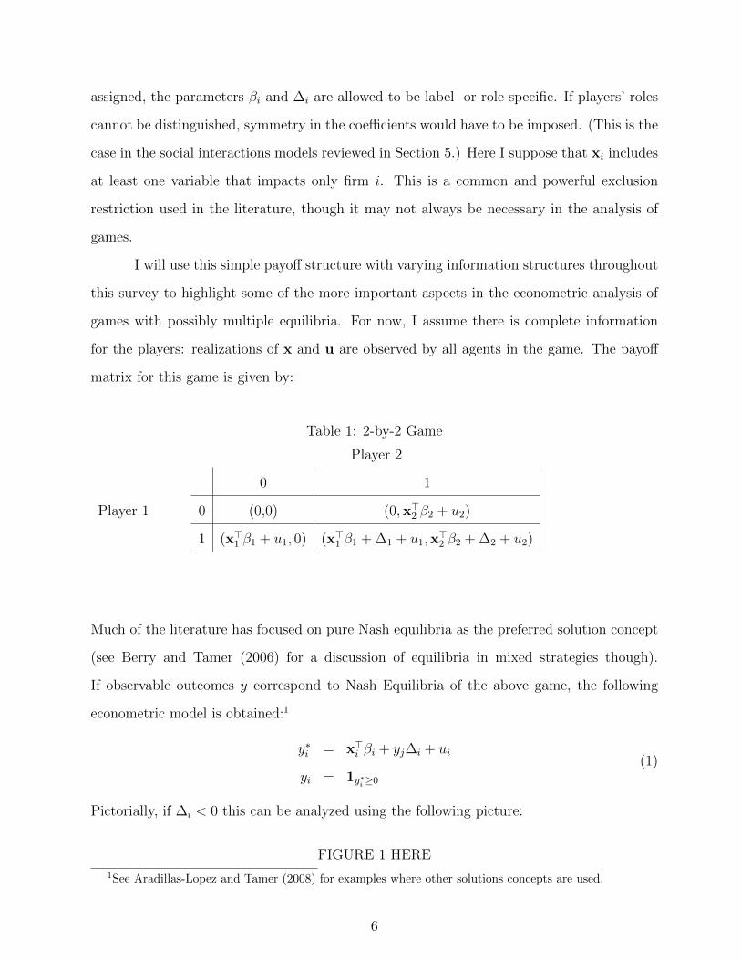
I will use this simple payo↵ structure with varying information structures throughout

this survey to highlight some of the more important aspects in the econometric analysis of

games with possibly multiple equilibria. For now, I assume there is complete information

for the players: realizations of x and u are observed by all agents in the game. The payo↵

matrix for this game is given by:

Table 1: 2-by-2 Game

Player 2

Player 1

0 1

0 (0,0) (0,x>2 �2 + u2)

1 (x>1 �1 + u1, 0) (x>

1 �1 +�1 + u1,x>2 �2 +�2 + u2)

Much of the literature has focused on pure Nash equilibria as the preferred solution concept

(see Berry and Tamer (2006) for a discussion of equilibria in mixed strategies though).

If observable outcomes y correspond to Nash Equilibria of the above game, the following

econometric model is obtained:1

y

⇤i = x>

i �i + yj�i + ui

yi = 1y⇤i �0

(1)

Pictorially, if �i < 0 this can be analyzed using the following picture:

FIGURE 1 HERE1See Aradillas-Lopez and Tamer (2008) for examples where other solutions concepts are used.

6

In the central region of the plane, the model predicts two possible solutions. What

is missing here is an “equilibrium selection mechanism” and in that sense the model is

“incomplete”. For payo↵ realizations within the region of indeterminacy (i.e., the central

region), one could imagine circumstances where (0, 1) is always selected or scenarios where

(1, 0) is always selected. Also possible are intermediary cases where with some probability

(potentially dependent on the realizations of x and u and the parameters in the model

✓ ⌘ (�1, �2,�1,�2)), say �(x,u, ✓) 2 [0, 1], one of the two equilibria is selected whenever

payo↵s fall in the multiplicity region. Di↵erent selection probabilities (i.e., �(x,u, ✓) in the

example) will induce di↵erent distributions over the observable outcomes yi.

One could (and in many examples below does) include the equilibrium selection mech-

anism into the structure. It is nevertheless important to bear in mind that modelling the

equilibrium selection process requires extra assumptions. This opens up an additional av-

enue for misspecification. Moreover, an estimated equilibrium selection mechanism is more

likely to be policy-sensitive. This is because “in a game with multiple equilibria, anything

that tends to focus the payers’ attention on one equilibrium may make them all expect it

and hence fulfill it, like a self-fulfilling prophecy. (. . . ) [T]he question of which equilibrium

would be focused on and played by real individuals in a given situation can be answered

only with reference to the psychology of human perception and the cultural background of

the players.” (Myerson (1991), pp. 108, 113) Consequently, a question that permeates much

of the literature on empirical games with possibly many equilibria is whether one can be

agnostic about the equilibrium selection rule, economizing on identifying assumptions, and

still be able recover the parameters of interest (i.e., ✓ in this example) or functions of these

parameters. Of course, many authors adopt a less pessimistic view than Myerson’s and point

out that certain equilibria, such as Pareto e�cient, risk-dominant or pure strategy equilibria,

are more salient and likely to be played than others. In the husband and wife example, for

instance, important papers in the intra-household allocation literature support the view that

Pareto ine�cient equilibria should not be selected. Inference methods that incorporate the

equilibrium selection mechanism may be informative about when and how certain equilibria

are likely to be played.

7

In his 1989 paper, Jovanovic stresses that multiplicity may or may not preclude point

identification. (It can be checked that without further restrictions the above example is

not point identified.) Certainly, even when the model is not point-identified, it may still

be partially (i.e., set) identifiable and informative about many issues of interest. What is

perhaps more intriguing is that multiplicity can, in some instances, help establish point

identification or make set-identified models more informative partly because it introduces

additional variation in the data (see, e.g. the discussion in Section 3.1 of Manski (1993)).

3 Games of Complete Information

In Section 2, I presented a two-player game where information is assumed to be complete:

both players know the realized values of all observable and latent variables (i.e., there is no

private information). Bresnahan and Reiss (1991) show that multiplicity (of pure strategy

Nash equilibria) will happen with positive probability in similar models of simultaneous

moves with more than two actions and two players if the support of the latent variables u

is large enough (e.g., ui 2 (�1,1)) (see Proposition 1 in Bresnahan and Reiss (1991)). To

keep matters simple, I keep with the example above with two actions (0 or 1) and two players.

In what follows I discuss various approaches to inference in games of complete information.

3.1 Pooling Multiple Equilibria Outcomes

If �i < 0, i = 1, 2, the entry of a firm in the market a↵ects the other firm’s profits negatively

and all equilibria in pure strategies for a given realization of u involve a unique number

y1 + y2 of players choosing 1. Let 1(N,x,u; ✓) be 1 if the number of players choosing 1 is N

for x,u and ✓. In this case, the likelihood conditional on x of observing N players choosing

1 is given by

P(N |x; ✓) =Z

1(N,x,u; ✓)P(du|x).

8

For the illustrative example in the previous section, we get

P✓(N = 0|x) = Fu1,u2(�x>1 �1,�x>

2 �2)

P✓(N = 2|x) = 1� Fu1(�x>1 �1 ��1)� Fu1(�x>

2 �2 ��2)

+Fu1,u2(�x>1 �1 ��1,�x>

2 �2 ��2)

P✓(N = 1|x) = 1� P✓(N = 0|x)� P✓(N = 2|x)

where u is assumed to be independent of x and Fu1,u2 is its known cdf. Given the assumption

of independence between x and u and known cdf Fu1,u2 , point identification can be ascer-

tained using arguments similar to those employed for parametric discrete choice models.

Once point-identification of ✓ is demonstrated, the model can be estimated via Maximum

Likelihood, under the assumption that �i < 0, with a random sample of games. This strat-

egy is pursued, for example, in Bresnahan and Reiss (1990) to identify and estimate a model

of firm entry in automobile retail markets and Berry (1992) for an entry model in the airline

industry. It also highlights the point that multiplicity is not necessarily an impediment to

identification. This happens because certain quantities (i.e. the number of entrants) are

invariant across equilibria when more than one solution is possible.

More generally, the key insight is that in this model certain outcomes can only occur

as unique equilibria. When �i < 0, i = 1, 2, this happens for y = (0, 0) and y = (1, 1).

This provides an avenue for identification and estimation of the model. In a coordination

game, where �i > 0, i = 1, 2, multiple (pure strategy) Nash equilibria occur whenever

u = (u1, u2) 2 [�x>1 �1 ��1,�x>

1 �1] ⇥ [�x>2 �2 ��2,�x>

2 �2]. In this case, both y = (0, 0)

and y = (1, 1) are possible equilibria. (y = (0, 0) is a unique equilibrium when ui <

�x>i �i ��i, i = 1, 2 and y = (1, 1) is a unique equilibrium when ui > �x>

i �i, i = 1, 2.) The

number of players choosing 1 is no longer the same across equilibria, but one could nonetheless

mimic the previous strategy and consider the probability of events {(0, 1)}, {(1, 0)} and

{(1, 1), (0, 0)}, where one pools together any two outcomes that are both equilibria for some

given x and u. Once this is done, singleton events correspond to outcomes that only occur

as unique equilibria regardless of the value taken by x and u.

The idea of identifying certain (non-exhaustive) outcomes with the occurrence of

9

multiple equilibria is pursued by Honore and de Paula (2010) for the identification of a

complete information timing game. In that paper, outcomes y are duration variables chosen

by individuals to model circumstances where timing decisions by one person a↵ect the payo↵

of another individual (e.g., joint migration, joint retirement, technology adoption). The

paper shows that multiplicity occurs only when duration spells terminate simultaneously for

both players (i.e., y1 = y2) and sequential spell terminations (i.e., y1 6= y2) occur only as

unique equilibria. Identification and estimation can then be achieved by considering those

events separately using standard arguments in the duration literature.

Unfortunately, this strategy is not always feasible in more general games as most

of the possible outcomes (if not all) might arise as equilibria alongside many other possible

solutions for a set of x and u with high probability. This would limit the ability of this insight

to achieve point-identification (though it might still allow for set-identification). Take for

instance the simple example in Jovanovic (1989). This example corresponds to the two-

action, two-player example from Section 2 with �1 = �2 = 0, � ⌘ �1 = �2 2 [0, 1) and

the pdf for u is f

u

(u1, u2) = 1(u1,u2)2[�1,0]2 (i.e., the latent variables are independently and

uniformly distributed on [�1, 0]). In this example, y = (0, 0) is a Nash equilibrium for any

realization of u. In addition, y = (1, 1) is also a Nash equilibrium for (u1, u2) 2 [��, 0]2.

(0, 1) or (1, 0) are never equilibria. Notice that (0, 0) arises as a unique equilibrium when

(u1, u2) /2 [��, 0]2, but also occur as equilibria alongside (1, 1) otherwise. Observation of y =

(0, 0) does not allow one to determine whether (u1, u2) were drawn in the region of multiplicity

(i.e., [��, 0]2) or not. Pooling the two outcomes as in the discussion above is hopeless for

(either point or set) identification (and consequently estimation) since P✓({(0, 0), (1, 1)}) = 1.

This is not an isolated example or a mere consequence of the lack of covariates: Bresnahan

and Reiss (1991) show that this problem is generally present for a wide class of discrete action

games (see Proposition 3 in that paper). In this case, pooling outcomes that are equilibria

for the same realizations of observed and latent covariates provides no identification leverage.

10

3.2 Large Support and Identification

An alternative strategy for point-identification of the parameters of interest in the presence

of multiplicity is provided by Tamer (2003), adapting similar ideas from the individual

discrete choice literature (e.g., Manski (1988) and Heckman (1990)). Consider models where

�1 ⇥ �2 < 0 for example. Figure 2 depicts the possible equilibria on the space of latent

covariates (u1, u2). In contrast with the case where �1 ⇥�2 > 0, any equilibrium is unique.

Nonetheless, there are no equilibria in pure strategies in the central region of the picture.

Tamer assumes that any outcome is possible in that area. One can rationalize this either

because players are thought to choose one of the outcomes in ways that are not prescribed

by the solution concept adopted here (Nash in pure strategies) or because the (unique)

equilibrium in mixed strategy places positive probability on every outcome y (though the

mixed strategy equilibrium probabilities are not incorporated into the econometric model).

Either way, we end up with an “incomplete” econometric model where the outcome of the

game in the central region is not resolved within the economic model. In this case, the

strategy from the previous subsection would be inconclusive as in Jovanovic’s example. This

is because it would bundle together all possible outcomes given that they are all allowed in

the central area of Figure 2.

FIGURE 2 HERE

Theorem 2 in Tamer’s paper nevertheless demonstrates the point-identification of the

parameter vector ✓ using exclusion restrictions and large support conditions on the observable

covariates. Without loss of generality, assume that �1 > 0 and �2 < 0. In this case, given

that games are identically and independently distributed and assuming that u is independent

of other covariates and has a known c.d.f., the following result holds:

Theorem 2 (Tamer 2003) Assume that for i = 1 or i = 2, there exists a regressor xik with

�k 6= 0 such that xik /2 xj, j 6= i and such that the distribution of xik|x�ik has everywhere

positive density, where x�ik = (xi1, . . . , xik�1, xik+1, . . . , xiK) and K is the dimension of

�i, i = 1, 2. Then the parameter vector ✓ = (�1, �2,�1,�2) is identified if the matrices

E[x1x>1 ] and E[x2x>

2 ] are nonsingular.

11

Here I only sketch the idea behind this result. Without loss of generality, assume

that �k > 0 (an analogous argument can be made for �k < 0). Because of the large

support condition, one can find extreme values of xik such that only unique equilibria in

pure strategies are realized (because P(ui > �� � x>i �i) ! 1 and P(ui > �x>

i �i) ! 1 as

xik ! 1). On the other �j 6= �

0j, j 6= i, the full rank condition on E[xjx>

j ] guarantees that

x>j �j 6= x>

j �0j with positive probability. This then implies that in the limit (as xik ! 1),

P�j(yj = 1|x) 6= P�0j(yj = 1|x) and the model identifies the parameter �j. Similar arguments

can be employed to demonstrate the identifiability of the remaining parameters. This point-

identification strategy can be extended to other contexts. Grieco (2012), for example, extends

it to a game of incomplete information where some variables are publicly observed by the

participants but not by the econometrician. I also note that the result uses the excluded

regressor xik in conjunction with the large support assumption. This is nonetheless not

necessary in more general contexts, for example when the payo↵ is not a linear function of

x for every player (see for example the generalization in Bajari, Hong, and Ryan (2010)).

The essence of this result is to find values of the regressor for which the actions of

all but one player are dictated by dominant strategies (regardless of the realizations of the

latent unobservable variables). This turns the problem into one of a discrete choice by the

single agent that does not play dominant strategies (given the covariates). The existence of

a regressor value that induces some of the players to always choose one action may be hard

to ascertain in many empirical contexts, but one may nevertheless get reasonably close to

that ideal.

Ciliberto and Tamer (2009), for example, estimate a firm entry model for the airline

industry where the distance between two airports a↵ects di↵erentially the decision of tra-

ditional carriers and discount airlines to operate a route between those two airports. They

find that distance carries a very negative e↵ect on the payo↵ for Southwest Airlines and

a mildly positive e↵ect on the payo↵ for traditional carriers. As they point out, “[t]his is

consistent with anecdotal evidence that Southwest serves shorter markets than the larger

national carriers” (p.1818). One could then think of markets where the distance between

airports is large as inducing a small probability of entry by Southwest and other discount

12

airlines but still providing variation in entry decisions by other, larger, carriers.

When the regressor values guaranteeing a dominant strategy for a subset of play-

ers cannot be obtained in an empirical application, other identification ideas need to be

employed. One feasible identification plan relies on bounds, focusing on a (possibly non-

singleton) set of parameters that are consistent with the model (see next subsection). In

that case, if the probability that certain players adopt dominant strategies gets larger, one

approaches the conditions for the point-identification strategy above and the identified set

of parameters gets smaller.

Because the point-identification result above relies on extreme values of the covariates,

even with the ideal conditions for Tamer’s result satisfied, this “identification at infinity”

strategy will have important consequences for inference as pointed out in Khan and Tamer

(2010), leading to asymptotic convergence rates that are slower than parametric rates as

the sample size (i.e., number of games) gets larger (see also the discussion in Bajari, Hahn,

Hong, and Ridder (2011)).2

Bajari, Hong, and Ryan (2010) incorporate the equilibrium selection mechanism into

the problem and demonstrate how large support conditions can help establish necessary

conditions for point-identification of the selection process. In expanding the model to in-

clude the equilibrium selection, they generalize the paper by Bjorn and Vuong (1984) where

equilibria are selected with a nondegenerate probability which is estimated along the other

payo↵ relevant parameters. Bajari, Hong and Ryan point out that “[e]stimating the selec-

tion mechanism allows the researcher to simulate the model, which is central to performing

counterfactuals”. Some caution is nonetheless warranted in justifying the policy-invariance

of the equilibrium selection mechanism in relation to the particular counterfactual of interest

as I indicate earlier (and also later) in this survey.

To maintain consistency with the discussion above, I assume that there are always

equilibria in pure strategy and remain in the two-player, two-action environment introduced

2The statement of Theorem 3 in Tamer (2003) is inaccurate. An additional term in the asymptotic

variance is missing, potentially invalidating the e�ciency claim in the result, as noted in Hahn and Tamer

(2004).

13

earlier. Bajari, Hong and Ryan nevertheless do allow for equilibria in mixed strategies (see

also Berry and Tamer (2006)), which are guaranteed to exist under more general conditions.

Let E(x,u, ✓) ⇢ {0, 1}2 be the set of equilibrium profiles given particular realizations of x

and u and value of ✓. Denote by �(y|E(x,u, ✓),x,u, ✓) the probability that y is selected

when the equilibrium set is E(x,u, ✓) given covariates at x and u and parameter ✓. The

distribution of latent variables F is known. When y is the unique equilibrium for the

realizations of x and u and parameter vector ✓, �(y|E(x,u, ✓),x,u, ✓) = 1. When it is

not an equilibrium, �(y|E(x,u, ✓),x,u, ✓) = 0. Finally, when there are other equilibria,

�(y|E(x,u, ✓),x,u, ✓) 2 [0, 1]. The conditional probabilities of actions are then

P(y|x; (✓, Fu

)) =

Z�(y|E(x,u, ✓),x,u, ✓)1

y2E(x,u,✓)fu(u)du (2)

where f

u

(·) is the pdf for u, which is assumed to be independent of x.

Given the specification summarised in (2), it is not clear whether the model identifies

the equilibrium selection mechanism �(·). As a matter of fact, unless further restrictions are

imposed, it does not. To take an extreme, but very simple illustration, consider again the

example in Jovanovic (1989) with no covariates. In this case, let � denote the probability

that (1, 1) is selected whenever there are multiple equilibria (i.e., (u1, u2) 2 [��, 0]2). Then,

P(y = (1, 1)) = ��2 and P(y = (0, 0)) = 1� P(y = (1, 1)).

It is not possible to pin down � and � from the distribution of outcomes. One of the issues

here is that there are more unknowns than equations. To reduce the degrees of freedom in

the problem, Bajari, Hong and Ryan impose additional structure. The first thing to note

is that the number of equations can be increased if the support of covariates x is relatively

large, generating additional conditional moments. To keep the number of parameters under

control, Bajari and co-authors assume that selection probabilities depend only on utility

indices through a relatively low-dimensional “su�cient statistic”. In essence this allows them

to parameterize the equilibrium selection mechanism as �(·) = �(·; �) for some parameter

� of relatively low dimension compared to the cardinality of covariate support. Once this

is guaranteed and exclusion restrictions like those in Tamer (2003)’s theorem above are

14

imposed, one can rely on there being at least as many conditional moments as there are

parameters (i.e., ✓ and �), which is necessary for identification (see their Theorem 3).

Of course, one should be careful not to introduce misspecifications while incorporating

the equilibrium selection mechanism into the econometric model (especially a parametric

one). Because the number of equilibria and the selection probability of an equilibrium may

depend on all variables observed by the players and the parameter ✓, the selection mechanism

should typically allow for this possibility. Any misspecification will likely contaminate the

estimation of ✓. Furthermore, it should be noted that the results in Bajari, Hong, and

Ryan (2010) provide necessary but not su�cient conditions for the point-identification of

the selection mechanism. Finally, as highlighted earlier, one ought to be careful not to

extrapolate the equilibrium selection mechanism in counterfactual experiments mimicking

policies that might a↵ect the way in which equilibria are selected.

If point-identification can be established, the authors suggest estimating the parame-

ters of interest using the conditional probability in (2) by the Method of Simulated Moments

(MSM) in order to handle the integration over the latent variables u. (As pointed out in

the text, the Simulated Maximum Likelihood (SML) method could also be applied here.)

Here the estimation procedure requires the determination of E(x,u, ✓) for given realizations

of x, u and values of ✓. Computing the whole equilibrium set becomes prohibitive already

with a relatively small number of players and actions. Bajari, Hong and Ryan also suggest

strategies to partly accommodate the computational issues.

With a random sample of g = 1, . . . , G games, one can then estimate the parameters

of interest using moments such as

E [(1yt=a � P(y = a|x; ✓, �, F ))h(x)] = 0

where h(·) are appropriately chosen weight functions of the observable covariates and a are

admissible action profiles. The sample analog of the above moment for the MSM estimator

is given byGX

g=1

⇣1yg=a � bP(y = a|x; ✓, �, F )

⌘h(x)

where bP is a computer simulated estimate of P.

15

3.3 Bounds

Typically the covariates’ support is not rich enough and the previous point-identification

strategy will not su�ce. Another avenue for inference in games with possibly multiple

equilibria is to rely on partial identification and use bounds for estimation. Take again

for instance the example in Jovanovic (1989) and note that P(y = (1, 1)) is at most �2

(if (1, 1) is always selected when (u1, u2) 2 [��, 0]2). Hence, because � < 1 we have

thatp

P(y = (1, 1)) � < 1. This is the set of all parameters � which are consistent

with the observable distribution of outcomes: for every � within [p

P(y = (1, 1)), 1) there

is an equilibrium selection probability that delivers the same distribution of observables.

Since P(y = (1, 1)) can be consistently estimated, one can estimate the identified set by

[q

bP(y = (1, 1)), 1).

This insight appears in Jovanovic’s discussion of this particular example and is ex-

plored in more detail by Tamer (2003). Consider the entry game in Section 2 for �i < 0, i =

1, 2. We were able to handle this case before using the fact that, whenever multiple equilib-

ria occur, the number of entrants is the same. In more general cases (e.g. when there are

more players and payo↵s are heterogeneous), this is not always the case even if we restrict

ourselves to pure strategy equilibria as noted in Ciliberto and Tamer (2009). We use this

simple example to illustrate the construction of bounds for the parameters of interest.

Remember that in this case (0, 0) and (1, 1) always occur as unique (pure) strategy

equilibria. Note also that

P(y = (0, 1)|x) 1� P(y = (1, 1)|x)� P(y = (0, 0)|x)

and

P(y = (0, 1)|x) � 1� P(y = (1, 1)|x)� P(y = (0, 0)|x)

�P�(u1, u2) 2 ⇥i=1,2[�x>

i �i,�x>i �i ��]|x

�

16

where, as before

P(y = (0, 0)|x) = Fu1,u2(�x>1 �1,�x>

2 �2) and

P(y = (1, 1)|x) = 1� Fu1(�x>1 �1 ��1)� Fu1(�x>

2 �2 ��2)

+Fu1,u2(�x>1 �1 ��1,�x>

2 �2 ��2).

The upper bound on P(y = (0, 1)|x) is attained if (0, 1) is always selected when (u1, u2) falls

in the region of multiplicity. Conversely, the lower bound is attained when (0, 1) is never

selected in that case. Hence, we subtract the probability that (u1, u2) falls in that region

from the previous probability. Similar bounds hold for P(y = (1, 0)|x). The bounds can be

modified to allow for mixed strategy equilibria as done in Berry and Tamer (2006).

These inequalities define a region of the parameter space where the true parameter

vector resides. When the covariates support is not as rich as outlined in the previous section

to guarantee point-identification, this set may (and typically will) be larger than a singleton.

Inference may nonetheless be carried out using methods developed in the recent literature

on estimation of partially identified models. Papers on the topic that pay special attention

to games with possibly multiple equilibria include Andrews, Berry, and Jia (2004), Ciliberto

and Tamer (2009), Beresteanu, Molchanov, and Molinari (2009), Pakes, Porter, Ho, and

Ishii (2011), Galichon and Henry (2011), Moon and Schorfheide (2012) and Chesher and

Rosen (2012). Other papers, more general in treatment, could also be cited and many of

the ideas can be applied to games under di↵erent information structures. Pakes, Porter, Ho,

and Ishii (2011), for instance, handle games where there is uncertainty which is symmetric

across players and information is complete as well as games of incomplete information (i.e.,

some information about payo↵s is private information to players). A thorough treatment of

the techniques in that literature would nonetheless be beyond the scope of this survey and

require much more space. For a recent introduction to that literature, see the survey by

Tamer (2010) and references therein.

17

3.4 Additional Topics

I close this section with a short discussion. First, much of the work dealing with multiplic-

ity has focused on discrete games. Many of the issues encountered in discrete games will

nevertheless also appear when the action space is continuous. These models are particularly

relevant in the study of pricing games among firms for example. If more than one solution

for a given realization of the payo↵ structure is possible, observed outcomes will be a mix-

ture over equilibria having the equilibrium selection mechanism as the mixing distribution.

Most of the ideas above can in principle be applied in those settings (see for instance the

discussion in Pakes, Porter, Ho, and Ishii (2011)), but more work in the future may reveal

further advantages or disadvantages of environments with continuous action spaces.

One notable reference in Econometrics focusing on continuous action spaces and mul-

tiple equilibria is Echenique and Komunjer (2009). They analyse a coordination game with

continuous actions and use equilibrium results typically found in the literature of supermod-

ular games. In this case, Tarski’s fixed point theorem can be employed to establish maximal

and minimal equilibria. Certain features of the structure under study (e.g., monotone com-

parative statics) can then be econometrically tested for using these extremal equilibria (see

also de Paula (2009) and Lazzati (2012) for econometric multi-agent models using Tarski’s

fixed point theorem and Molinari and Rosen (2008) for a discussion of identification in super-

modular games with discrete actions). A similar environment (with payo↵ complementarities

and discrete action space) also appears for the empirical analyses of Ackerberg and Gowrin-

sankaran (2006) (where an equilibrium selection mechanism with support on the best and

worst equilibria is incorporated incorporated into the econometric model) and of Jia (2008)

(where one of the extremal equilibria is assumed to be selected). Jia (2008) also exploits a

constructive version of Tarski’s theorem for computation.

4 Games of Incomplete Information

The previous section presented ideas for the analysis of games of complete information.

There, individuals are assumed to know the payo↵ realizations of every other player. This

18

is nevertheless not always a good assumption. In the case of firms contemplating entry into

a particular market, at least some part of the cost structure is private information to each

firm. It turns out that games where information is incomplete and agents possess at least

partially private information about payo↵s provide di↵erent avenues for identification and

estimation of the structure of interest when there are multiple equilibria.

I start with the same payo↵ structure as in the example from Table 1, but assume

that ui is known only to person i, where i = 1, 2. As in the previous section, I assume

that roles or labels can be assigned to players. Given realizations of x and u, agents now

decide on their actions based on the payo↵s they expect, given the distribution of “types”

for the other individual involved in the game (i.e. the private information components of

their payo↵s, ui). As before, I consider only pure strategy equilibria for simplicity. Given i’s

opponent’s strategy, her best response dictates that

yi = 1 if x>i �i + P(yj = 1|x, ui)�i + ui � 0, j 6= i (3)

and 0 otherwise. The term “P(yj = 1|x, ui)” accommodates i’s beliefs about the other

person’s type given her information set (comprising x and ui) and the other person’s strategy

about choosing 0 or 1. A Bayes-Nash equilibrium (in pure strategies) is characterized by

mutual best reponses of players 1 and 2 and consistent beliefs.

When information is incomplete, the expression above highlights the fact that the

joint distribution of the latent variables (u1, u2) plays an important role. Unless these vari-

ables are independent, P(yj = 1|x, ui) will be a non-trivial function of ui, i = 1, 2. When u1

and u2 are not independent, player i’s type (i.e., ui) is informative about her opponents type

(i.e., uj), and in equilibrium, will likely a↵ect what she expects her opponent to play. If,

on the other hand, u1 ?? u2|x, i’s expectations about j’s action will not depend on ui since

her type brings no hint about uj. Because, conditional on x, the equilibrium yi depends

solely on ui, this assumption also implies that y1 and y2 are conditionally independent given

x for a particular equilibrium. Unless otherwise noted and except for the last segment in

this section, I will assume that the private shocks are (conditionally) independent within a

game. In this case, we can write P(yj = 1|x, ui) = pj(x) and equilibrium choice probabilities

19

should solve the following system of equations:

pi(x) = 1� Fui|x(�x>i �i � pj(x)�i|x), i = 1, 2, i 6= j. (4)

This system can easily be seen to admit multiple solutions. Assume for example a sym-

metric payo↵ structure such that �1 = �2 = 10.5, u1 and u2 follow independent logis-

tic distributions and x>1 �1 and x>

2 �2 are drawn such that x>1 �1 = x>

2 �2 = �3.5. Then,

p1(x) = p2(x) = 0.047 and p1(x) = p2(x) = 0.204 are symmetric solutions to the system

above. (A third solution where both players choose 1 with probability close to 1 also exists.)

In general the constituents of this model are not point-identified. To see this, denote

by E(x, ✓, F ) the set of equilibria for a given realization of x and primitives (✓, F ). Note that

the equilibrium set now depends not on u (which are only privately observed) but on its

distribution. Because for now I retain the assumption that u1 ?? u2|x, recall that in equilib-

rium y1 and y2 are conditionally independent, and an equilibrium is hence characterized by

the marginal distributions of yi given x, i = 1, 2. Let (pk1(x), pk2(x))

|E(x,✓,F )|k=1 be an ordering of

the equilibrium set E(x, ✓, F ). Then, the distribution of outcomes conditional on covariates

x is given by

P(y1, y2|x) =|E(x,✓,F )|X

k=1

�(k|E(x, ✓, F ),x, ✓, F )pk1(x)y1(1� p

k1(x))

1�y1p

k2(x)

y2(1� p

k2(x))

1�y2,

where �(·) is the equilibrium selection mechanism and places probability �(k|E(x, ✓, F ),x, ✓, F )

on the selection of equilibrium k. This is a mixture of independent random variables and

results such as those in Hall and Zhou (2002) can be used to demonstrate that the compo-

nent distribution (pk1(x), pk2(x))

|E(x,✓,F )|k=1 and mixing probabilities are not point-identified by

the model if |E(x, ✓, F )| is strictly greater than 2. Similar results can be obtained for more

players (using Hall, Neeman, Pakyari, and Elmore (2005), for example): if the number of

equilibria on the support of the selection mechanism is large relative to the number of play-

ers, the structure is not point-identified by the model (see for instance the Supplementary

Appendix in de Paula and Tang (2012)).

As I did in the previous section, I now discuss di↵erent approaches to inference in

games of incomplete information like the one I just outlined.

20

4.1 Degenerate Equilibrium Selection Mechanism

The previous discussion underscores the benefits of further restrictions on the equilibrium

selection mechanism for the econometric analysis of incomplete information games with

possibly many equilibria. One common strategy is to assume that

�(k|E(x, ✓, F ),x, ✓, F ) = 1k=K

for some K 2 E(x, ✓, F ). In words, whenever primitives and covariates coincide for two

games, thus inducing an identical equilibrium set, the same equilibrium is played in these

two games. One can nevertheless be agnostic about which equilibrium is selected (i.e., which

element of E(x, ✓, F ) is selected).

When is it realistic to assume that the same equilibrium is played across games? As

Mailath (1998) points out, “[t]he evolution of conventions and social norms is an instance

of players learning to play an equilibrium”. If an equilibrium is established as a mode of

behavior by past play, ‘custom’ or culture, this equilibrium becomes a focal point for those

involved. When observed games are drawn from a population which is culturally or geo-

graphically close, sharing similar norms and conventions, one would expect this assumption

to be adequate.

If a single equilibrium occurs in the data for every given payo↵ configuration, this

restriction essentially allows one to treat the model in standard ways for identification and

inference. Once identification is guaranteed, one possible strategy for estimation is the two-

step estimator proposed in Bajari, Hong, Krainer, and Nekipelov (2010). The strategy builds

on the earlier work by Hotz and Miller (1993) for the estimation of empirical (individual)

dynamic discrete choice models and later on by Aguirregabiria and Mira (2007) and Bajari,

Benkard, and Levin (2007) for dynamic games (where information is incomplete). It also

resembles estimators proposed in the social interactions literature and covered below. I de-

scribe the procedure using the example from Table 1 (still with conditionally independent

latent variables u1 and u2). Bajari, Hong, Krainer, and Nekipelov (2010) present the method

in more generality.

21

STEP 1. In a first step, the (reduced form) conditional choice probabilities for the vari-

ous outcomes in the action space are estimated nonparametrically: bP(yi|x), i = 1, 2. This

can be done using sieves or kernel methods.

STEP 2. In the second step, estimates for the structural parameters are obtained from

the conditional choice probability estimates. If a unique equilibrium is played in the data for

same realizations of the payo↵ matrix, pi(x) and the expected payo↵ for player i of choosing

1 using equilibrium beliefs (i.e., x>i �i + pj(x)�i) are in one-to-one correspondence. In the

example this correspondence is simply obtained as

x>i �i + pj(x)�i = �F

�1ui|x(1� pi(x)|x).

Given a sample of G iid games, the estimation then proceeds to minimize the following least

squares function with respect to ✓:

GX

g=1

h�F

�1ui|x(1� bpi(xg)|xg)� x>

ig�i � bpj(xg)�i2

h(xg)

where h(·) is again an appropriately chosen weight function. Under adequate conditions the

estimator for ✓ converges at parametric rates as pointed out in the paper.

The assumption of a unique equilibrium in the data is crucial to travel from the

conditional choice probabilities to the second-step estimator as it guarantees (together with

other additional restrictions) that pi(x) and the expected payo↵ for player i of choosing 1

using equilibrium beliefs (i.e., x>i �i+pj(x)�i) are in one-to-one relationship. Because of this

the above procedure bypasses the calculation of all equilibria for each possible value of ✓ much

as Hotz and Miller (1993) avoids to computation of a dynamic program in the estimation of

individual dynamic discrete choice models. Of course, as long as there is a unique selected

equilibrium in the data, other estimators which rely on uniqueness such as Aradillas-Lopez

(2010) can also be used. The assumption is also employed for example in Kasy (2012), which

proposes a procedure to perform inference on the number of feasible equilibria in a game:

even if the equilibrium selection mechanism is assumed to be degenerate, once the primitives

22

(i.e., (�1, �2,�1,�2) in my example, but more general non-parametric functions in Kasy

(2012)) are estimated, one can infer the number of equilibria for the estimated particular

payo↵ structure at given realization of covariates.

I should note that, as discussed in Bajari, Hong, Krainer, and Nekipelov (2010),

when covariates x have a continuous support, the requirement that the data come from a

unique equilibrium imposes subtle additional restrictions as the implementation of the above

estimation strategy typically demands smoothness of the first stage estimator with respect

to the covariates. Figure 3 sketches the possible ways in which this prerequisite might fail.

The horizontal axis represents a generic continuous covariate x 2 R and the vertical axis

schematically represents the equilibrium conditional choice probabilities p(x). The graph

sketches the potential equilibrium probabilities corresponding to each x. For x > x

0, there

are three potential equilibria whereas for x < x

0, there is only one. The red line marks the

equilibrium that is selected in the data and stands for a possible (degenerate) equilibrium

selection mechanism. Because the number of equilibria |E(x, ✓, F )| may change with x as

in the scheme below, small changes in the covariates may provoke abrupt changes in the

cardinality of the equilibrium set. In the figure this happens around x

0. At this bifurcation

point, the equilibrium conditional choice probability selected p(x) may vary non-smoothly as

is the case for the equilibrium selection mechanism. An implicit condition then is that such

bifurcations happen in ways that do not a↵ect the estimation. It is also possible that minute

changes in the covariates x may tip the selection of the equilibrium observed in the data in

a discontinuous manner. For the scheme in the figure this happens at x

00. Both points (x0

and x

00) present possible challenges to the smoothness requirement.

FIGURE 3

In the presence of non-smooth equilibrium selection mechanisms, the two-step estimator

suggested above will perform poorly. Aguirregabiria and Mira (2008) produce some Monte

Carlo evidence of the de�ciencies of this estimator when there are discontinuities in the

equilibrium selection mechanism and suggest an alternative strategy, combining a Pseudo

Maximum Likelihood estimator with a Genetic Algorithm.

23

The assumption of a degenerate equilibrium selection mechanism is usually invoked

as well in the estimation of dynamic incomplete information games. In these environments,

an action profile a↵ects not only the players payo↵s, but also the evolution of the state vari-

ables. The prescribed equilibrium strategies in this case generalize (3) to account for future

repercussions. Common estimation strategies for dynamic games such as Aguirregabiria and

Mira (2007), Bajari, Benkard, and Levin (2007), Berry, Pakes, and Ostrovsky (2007) and

Pesendorfer and Schmidt-Dengler (2008) adapt well-known procedures for the estimation of

single-agent Markov decision problems such as Hotz and Miller (1993). In essence, these

estimators will rely on the existence of a one-to-one mapping between value functions and

conditional choice probabilities. For this to hold, they rely on there being a single equilib-

rium in the data for games with identical payo↵ realizations as well as other assumptions

usually invoked to guarantee the existence of such mapping (e.g., additive separability of ui).

4.2 Identifying Power of Multiplicity

Sweeting (2009) follows a di↵erent route and incorporates the equilibrium selection mecha-

nism in the estimation (see references in the previous section for similar strategies in complete

information models).

He studies coordination (or not) on the timing of commercial breaks among radio

stations (i.e. players) within a geographical market (i.e. game). In terms of the application

in his paper the intution is as follows. “If stations want to coordinate then there may be

an equilibrium where stations cluster their commercials at time 1 and another equilibrium

where they cluster their commercials at time 2. (. . . ) If stations want to play commercials

at di↵erent times then we would expect to observe excess dispersion within markets (mar-

ket distributions less concentrated than the aggregate) rather than clustering.” (p.713 in

Sweeting (2009))

In his discussion, he focuses on symmetric (stable) pure strategy Bayesian Nash equi-

libria in a coordination game. To keep matters simple, I consider again the two-player game

with payo↵ structure from Table 2. Assume that x>i �i = ↵, i = 1, 2 and � = �1 = �2 � 0.

As has been the case up to this point, private information is assumed to be independent

24

across agents and from x. Given the parametrization in his model, multiplicity always pro-

duces three symmetric equilibria, two of which are stable. Denote the choice probabilities in

these two stable equilibria p

l and p

h, where pl < ph.

To “complete” the model, Sweeting assumes that the stable equilibria are selected

with probability �k, k = l, h, whereas the unstable equilibrium is never selected. The outcome

probability is then

P(y1, y2|x) =X

k=l,h

�k

0

@ 2

y1 + y2

1

A (pk)y1+y2(1� p

k)2�y1�y2, �l + �h = 1. (5)

Notice that with a unique equilibrium in the data, (5) corresponds to the distribution of

a binomial random variable (with parameters 2 and p). Using simulations, Sweeting notes

that “a mixture generates greater variance in the number of stations choosing a particular

outcome than can be generated by a single binomial component” when � > 0 (see p.723 in

his paper). As he points out, this suggests that multiplicity provides additional information

about the payo↵ structure of the game under analysis.

de Paula and Tang (2012) formalize and generalize this idea in many directions. For

the basic insight, take expression (4) and compare two equilibria where p

hj (x) > p

lj(x). If

�i > 0, it has to be the case that phi (x) > p

li(x). (This is because Fui|x is increasing since

it is a cdf.) On the other hand, if �i < 0 one must have p

hi (x) < p

li(x). With two players,

multiple equilibria are possible only if both �1 and �2 have the same sign (in contrast with

the complete information case). Consequently, if �1 and �2 are positive, ph1(x) > p

l1(x) if

and only if ph2(x) > p

l2(x). In other words, the equilibrium choice probabilities by player 2

are an increasing function of the equilibrium choice probabilities by player 1. Conversely,

when both �1 and �2 are negative, the equilibrium choice probabilities by player 2 are

a decreasing function of the equilibrium choice probabilities by player 1. Because of this

monotonicity, the correlation of player actions across games will be positive when both �1

and �2 are positive and negative otherwise. Interestingly, because private types ui = 1, 2

are assumed to be independent (conditionally on x), if there is only one equilibrium in the

data the actions will be uncorrelated and uninformative about �i, i = 1, 2. This gives the

following specialization of Proposition 1 in de Paula and Tang (2012)):

25

Proposition 1 (de Paula and Tang (2012)) Suppose u1 ?? u2|x. (i) For any given x,

multiple equilibria exist in the data-generating process if and only if E[y1y2|x] 6= E[y1|x]E[y2|x];

and (ii) if that is the case for some x,

sign (E[y1y2|x]� E[y1|x]E[y2|x]) = sign(�i), i = 1, 2

In the paper, the baseline utility x>i �i can be replaced by a generic function of xi and

the parameter �i is also allowed to depend on xi, but I keep with the payo↵s in Table 2 for

simplicity and consistency. The result also holds for an arbitrary number of players and allows

for asymmetric equilibria and situations where the number of equilibria is unknown. (Kline

(2012) recently extends the idea of this result to environments with complete information.)

The subtle implication of the proposition is that multiplicity is informative about

aspects of the model in ways that uniqueness is not. Of course, for the set of covariate values

where there is only one equilibrium in the data the estimation can then be performed under

various restrictions on utilities, �i, i = 1, 2 and F

u|x (see Aradillas-Lopez (2010), Berry and

Tamer (2006), and Bajari, Hong, Krainer, and Nekipelov (2010) for more details).

For games with more than two players, de Paula and Tang (2012) rely on this result

to suggest a test for the hypothesis that there are multiple solutions in the data and, condi-

tional on there being more than one equilibrium, on the sign of �i, i = 1, 2. To implement

this test, they build on recent developments in the statistical literature on multiple com-

parisons (Romano and Wolf (2005)) (see the recent survey by Romano, Shaikh, and Wolf

(2010)). Because the test proposed relies on conditional covariances, with discrete covariates

it is implementable using well-known results in the multiple testing literature. Based on

his model, Sweeting (2009) also suggests tests for multiple symmetric equilibria when the

cardinality of the equilibrium set is known. The first is based on calculating the percentage

of pairs of players whose actions are correlated. The other is a test of the null of a unique

equilibrium against the alternative of exactly two equilibria using MLE.

Finally, I should note that the essential assumption of conditional independence of

the latent variables u is also commonly found in dynamic games of incomplete information.

Optimal decision rules in those settings involve not only equilibrium beliefs but continuation

26

value functions that may change across equilibria. Nevertheless, the characterization of

optimal policy rules in that context suggests that the existence of a unique equilibrium in

the data can still be detected by the lack of correlation in actions across players of a given

game as presented in the current paper much as in the static game. (The identification of

sign(�i) would require additional restrictions though.) Because most of the known methods

for semi-parametric estimation of incomplete information (static or dynamic) rely on the

existence of a single equilibrium in the data (see above), a formal test for the assumption of

a unique equilibrium in the data-generating process can be quite useful.

4.3 Game Level Heterogeneity and Correlated Private Signals

To establish Proposition 1 in de Paula and Tang (2012), it is paramount that the latent

variables be conditionally independent. Any association between u1 and u2 will lead to cor-

relation in actions even under a unique equilibrium but also change the nature of equilibrium

decision rules in important ways (i.e., P(yj = 1|x, ui) in (3) is now a non-trivial function of

ui). Aradillas-Lopez (2010) suggests in a subsection an estimation procedure to handle cases

allowing for correlated private values, but relies on the assumption that a single equilibrium

is played in the data. Another example is Wan and Xu (2010), who nevertheless also require

that a unique (monotone) Bayesian-Nash equilibrium be played in the data. As long as one

is comfortable with the assumption of a single equilibrium in the data described previously,

these methods can be used for estimation. To my knowledge, general results along the lines

of de Paula and Tang (2012) that allow for both correlation of private values and multiplicity

have not been proposed (though see the working paper version of that article for a discussion

of some possible characterizations).

One empirically important form of association between latent variables that has never-

theless received some attention amounts to decomposing ui into a public observed component

✏i and a privately observed component ⌫i. Whereas we retain the assumption that ⌫1 and

⌫2 are (conditionally) independent, I assume for simplicity that the publicly observed errors

take the form of a game-level shock ✏1 = ✏2 = ✏. In the empirical games literature, the pres-

ence of this “market” level shock is typically referred to as unobserved heterogeneity (even

27

though ⌫1 and ⌫2 are themselves heterogeneous and unobserved within and across games).

The presence of ✏ prevents one from employing the results in de Paula and Tang

(2012) much as the correlation in fully private u1 and u2 would. The practical solution is

nevertheless to account for it by modelling the distribution of publicly observed latent shocks

when a cross-section is employed or using a “market-invariant” fixed or (possibly correlated)

random e↵ect again under the assumption that a unique equilibrium occurs in the data for

each particular market when panel data is available. In a dynamic context, Aguirregabiria

and Mira (2007) for instance introduce game level shocks as a correlated random e↵ect with

finite support (in the tradition of Heckman and Singer (1984) for duration models). Grieco

(2012) also models the distribution of publicly observed shocks in a static game estimated

on a cross-section.

Alternatively Bajari, Hong, Krainer, and Nekipelov (2010) note that “[i]f a large panel

data with a large time dimension for each market is available, both the nonparametric and

semiparametric estimators can be implemented market by market to allow for a substantial

amount of unobserved heterogeneity” (p.475). The requirement of a long panel helps cir-

cumvent the incidental parameters problem in this fairly nonlinear context. It should also be

noted that, provided the equilibrium is the same for the di↵erent editions of the game within

a particular “market”, di↵erent equilibria are allowed across di↵erent markets. Similar ideas

also appear in other papers of the literature such as Bajari, Benkard, and Levin (2007) or

Pesendorfer and Schmidt-Dengler (2008). Even in the absence of long panels, Bajari, Hong,

Krainer, and Nekipelov (2010) suggest a few interesting strategies such as the use of condi-

tional likelihood methods when the ⌫ errors are logistic or the use of Manski (1987)’s panel

data rank estimator. These proposals are nevertheless not further developed in that paper

and some caution might be warranted given the simultaneous equation nature of the problem

(i.e., the presence of pj(x) among the regressors in (4) might have repercussions for the two

step procedure since pj(x) is also a↵ected by the game level shock ✏).

28

5 Models of Social Interactions

Social interaction models have gained widespread attention since Manski (1993). Whereas

that paper focused on linear social interaction systems where equilibrium is unique, Brock

and Durlauf (2001) and Brock and Durlauf (2007) consider a model of social interactions

with discrete choices where multiple equilibria are possible. In the model, the value of

a particular choice depends on the distribution of actions among other individuals in the

community. In what follows I adapt the expressions in Brock and Durlauf’s papers to keep

with the previous notation here. Normalizing the value of choosing zero to 0, the utility

obtained from choosing 1 can be written as

gi(P(y�i|x),x, ✓) + ui

(see page 238 in Brock and Durlauf (2001). The term gi(P(y�i|x),x, ✓) encompasses what

Brock and Durlauf call the private and the social utilities attached to this particular choice

(or, given our normalization, the di↵erence in those utilities of choosing 1 over 0). The

social utility depends on the conditional probability that i places on the choices of others

when making her choice. As before, ui is a random utility component which is known to the

individual but unknown to others and is identically and independently distributed across

agents. Typically, ui is taken to be logistically distributed.

The probability distribution that i puts on the choices of others is denoted by P(y�i|x)

and is determined in equilibrium. Person i’s choice is then given by

yi = 1 if gi(P(y�i|x),x, ✓) + ui � 0. (6)

As with incomplete information games, an equilibrium will consist of mutual best responses

and self-consistent beliefs. Given the nonlinearities in the model, multiplicity is again a

possibility. Note nevertheless that instead of comparing (equilibrium) expected utilities as

in (3), the expression above compares utility functions that depend on the (equilibrium) dis-

tributions of actions. These two will di↵er for general parameterizations (possibly nonlinear

in P). This is the case, for example, when there is preference for conformity as discussed in

Brock and Durlauf (2001) (p.239). This is an important distinction. In the main (linear)

29

parameterization considered in that paper, they nevertheless coincide. This specification

postulates that

gi(P(y�i|x),x, ✓) = x>i � +�E

Pj 6=i yj

N � 1

���x�

where N is the group size as before and � and � are parameters to be estimated. Because

x>i � +�E

Pj 6=i yj

N � 1

���x�= E

x>i � +�

Pj 6=i yj

N � 1

���x�,

the (equilibrium) expected utility agrees with the utility at the expected (equilibrium) profile

of actions. This is in particular the best response predicament in my example with two

players and two actions under incomplete information when �1 = �2 and �1 = �2. A

noteworthy di↵erence between this setup and that in the previous section is that I do not

assume that players’ roles or labels (e.g., firm identity, husband or wife) can be assigned.

This “anonimity” assumption is more natural in the social interactions systems where a large

number of people is typically observed per group.

Because the equilibrium moment EhP

j 6=i yj/(N � 1)���xiis observable, it can be esti-

mated by the average choice in this particular game and equilibrium (e.g., Brock and Durlauf

(2007), p.58). When there is a small number of players (as is the case in Industrial Orga-

nization applications for example), the choice probabilities will not be reliably estimated

by averaging choices within a game. In this case some combination of observations across

games is unavoidable and I refer the reader to the discussion in the previous section. For

most applications of social interaction models however, the number of agents within a game

is much larger. Consequently, the average peer choice in a game will consistently estimate

the average action within the game (see Proposition 6 in Brock and Durlauf (2001)). Because

average peer choice will display little variability within a group, variation across games can

then be exploited to estimate � and �.

I now briefly discuss estimation and additional topics in this class of models in two

di↵erent subsections.

30

5.1 Estimation

In this context, two alternative estimators are suggested in Bisin, Moro, and Topa (2011)

(building on Moro (2003)). The first procedure estimates the game via Maximum Likelihood

imposing the self-consistency equilibrium conditions. Because here a parameter vector might

induce multiple equilibria for a given data set, the estimation proceeds by selecting that

equilibrium which maximizes the likelihood (for a given parameter vector) and subsequently

maximizing the likelihood function over the parameter space. (This resembles the procedure

suggested in Chen, Tamer, and Torgovitsky (2011) which suggests profiling the equilibrium

selection mechanism in a sieve-Maximum Likelihood procedure.) The second procedure is a

plug-in estimator where EhP

j 6=i yj/(N � 1)���xiis replaced by the average peer choice within

the game and parameters are then estimated via Maximum Likelihood. The log-likelihood

function in the case of my example is given by:

GX

g=1

X

i2g

ln

1� Fu

✓�x>

i � ��

Pj 6=i,j2g yj

N � 1

◆�,

where i 2 g indicates that person i belongs to neighborhood g. This estimator can be

seen as a two-step estimator akin to the procedure outlined in the previous section for

incomplete information games. As was the case in the previous section, this estimator

avoids the calculation of all the equilibria for a given parameter value. In response to the

computational di�culties that this entails, they advise using the two-step estimator as an

initial guess in the direct estimator. Similar two-step procedures with (possibly) group-

level unobservables are also suggested by Shang and Lee (2011). Bisin, Moro and Topa

present Monte-Carlo evidence in a model with possibly many equilibria for certain parameter

configurations that highlights the computational costs and statistical properties of the two

estimators. Because the asymptotic approximations rely on N ! 1, I must also point out

that the econometric estimators in such large population games might present some delicate

issues given the dependence in equilibrium outcomes within a game as the number of players

grows. This is a topic of ongoing research (see, for example, Menzel (2010) and Song (2012)).

31

5.2 Additional Topics

As was the case in the previous section, group level unobserved heterogeneity is potentially

important in many applications. Ignoring it essentially rules out an important channel of

unobserved contextual e↵ects (or correlated e↵ects) in the terminology coined by Manski

(1993). Section 4 of Brock and Durlauf (2007) also discusses a series of potential scenarios

that would allow the model to identify (at least partially) the parameters of interest. Those

include the use of panels, restrictions on the distribution of unobserved group shocks (i.e.,

large support, stochastic monotonicity, unimodality) as well as other features of the model

(i.e., linearity in terms of group shocks). Some of these restrictions may also be useful in the

incomplete information games described previously.

6 Discussion

I will finish this survey with a brief discussion on post-estimation analysis, potential areas

of development and applications.

6.1 Counterfactuals and Post-Estimation

Once in possession of point- or set-estimates for the parameters of interest, one may be

interested in the e↵ect of counterfactual policies. This goal is after all behind the very

development of the Cowles Comission agenda delineated in the beginning of this article. If

the equilibrium selection mechanism is included in the structure as an estimation object, one

has a complete model which can be simulated to generate counterfactual distributions after

the introduction of alternative policies (see, e.g., Bajari, Hong, and Ryan (2010), p.1537).

As pointed out earlier, one must nevertheless be cautious about the policy-invariance

of the estimated equilibrium selection mechanism. Quoting Berry, Pakes, and Ostrovsky

(2007), “though our assumptions are su�cient to use the data to pick out the equilibrium

that was played in the past, they do not allow us to pick out the equilibrium that would

follow the introduction of a new policy. On the other hand, the (. . . ) estimates should

32

give the researcher the ability to examine what could happen after a policy change (say, by

examining all possible post-policy-change equilibria)” (p.375). This is done for example in

Ciliberto and Tamer (2009) where a range of possible counterfactual outcomes is provided for

an intervention repealing a particular piece of legislation on the entry behavior of airlines in

their empirical analysis. Of course, any counterfactual analysis (with or without an estimated

equilibrium selection policy) would require the computation of all equilibria though only for

the range of parameters estimated.

An additional motivation for including the equilibrium selection mechanism as an

estimation object is to retrospectively learn about the process and covariates determining

which equilibria come to be played in the data. Even when the game is estimated under

the assumption that a unique equilibrium is played in the data, possession of estimated

parameters allows one to go back and calculate all the potential equilibria for a particular

parametric configuration. In their study of stock analyst’s recommendations, for instance,

Bajari, Hong, Krainer, and Nekipelov (2010) notice the existence of multiple equilibria before

General Attorney Eliot Spitzer of New York launched a series of investigations on conflict of

interest, one of these equilibria yielding much more optimistic ratings than those granted in

the equilibrium post-Spitzer.

6.2 Potential Avenues for Future Research

In the previous sections I tried to present many of the tools used in the econometric analysis

of games with multiple equilibria. There are nevertheless still much to be understood in

these settings. One interesting avenue which appears in some of the papers cited here is the

connection with panel data methods. There, just as under multiplicity the distribution of

outcomes in game theoretic models is a mixture over equilibrium-specific outcome distribu-

tions, the observable distribution of outcomes in panel data models is a mixture over the

distribution of individuals e↵ects. Important idiosyncrasies such as the (typical) finiteness

of the equilibrium set (which would correspond to a finite support for the individual e↵ects)

may help bring in interesting technical results in the panel literature to shed light into some

of the properties of econometric game theoretic models. Examples of studies in that vein

33

are Hahn and Moon (2010) and Bajari, Hahn, Hong, and Ridder (2011). Here a important

caveat already mentioned earlier is that the cardinality of the equilibrium set, |E(✓, F,x)|,

will depend on the covariates and parametric configurations whereas the support of the indi-

vidual e↵ects in the usual panel data model su↵ers no such restrictions. This might introduce

important complications.

In a similar fashion, Grieco (2012) and Chen, Tamer, and Torgovitsky (2011) suggest

treating the equilibrium selection mechanims as a (possibly infinite dimensional) nuisance

parameter which is concentrated out in a profile sieve-MLE procedure aimed at estimating

semiparametric partially identified models. Again in this case, the dependence of the the

cardinality of the equilibrium set, |E(✓, F,x)|, on the covariates and parametric configurations

might introduce subtle complications as the class of functions which contain the equilibrium

set might have to vary with ✓, F and x to accommodate this dependence.

6.3 Applications

Here I discussed some of the commonly analyzed models where multiplicity shows up promi-

nently in the econometric analysis of games and the usual procedures to handle this feature.

I left out other models where nonuniqueness is rampant but so far have been given less

attention. One example are static models of network formation a la Jackson and Wolinsky

(1996). Whereas the solution concepts used in that literature di↵er from those used in the

non-cooperative games studied above, it is not not uncommon to encounter many possible

stable networks for a given payo↵ configuration. Those di�culties are perhaps compounded

in econometric analogs of network formation models because equilibrium existence results

for heterogenous payo↵s are less readily available in the theory literature and computational

challenges in their analysis are notorious.

For space considerations, I have only briefly mentioned empirical applications and

focused on more methodological aspects of the analysis. Many of the papers cited here nev-

ertheless provide (or actually even focus) on empirical questions (e.g., Sweeting (2009) or

Ciliberto and Tamer (2009)) and many other examples in the empirical IO or peer e↵ects

literatures can be enumerated. Recent applications in other areas of Economics are never-

34

theless available (e.g., Card and Giuliano (2011) or Todd and Wolpin (2012)) and are likely

to become more common.

35

References

Ackerberg, D., and G. Gowrinsankaran (2006): “Quantifying Equilibrium Network

Externalities in the ACH Banking Industry,” Rand Journal of Economics, 37, 738–761.

Aguirregabiria, V., and P. Mira (2007): “Sequential Estimation of Dynamic Discrete

Games,” Econometrica, 75(1), 1–53.

(2008): “Structural Estimation of Games with Multiple Equilibria in the Data,”

Working Paper.

Andrews, D., S. Berry, and P. Jia (2004): “Confidence Regions for Parameters in

Discrete Games with Multiple Equilibria, With an Application to Discount Chain Store

Location,” Working Paper.

Aradillas-Lopez, A. (2010): “Semi-parametric Estimation of Simultaneous Games with

Incomplete Information,” Journal of Econometrics, 157(2), 409–431.

Aradillas-Lopez, A., and E. Tamer (2008): “The Identification Power of Equilibrium

in Simple Games,” Journal of Business and Economic Studies, 26, 261.

Bajari, P., L. Benkard, and J. Levin (2007): “Estimating Dynamic Models of Imper-

fect Competition,” Econometrica, 75, 1331–1370.

Bajari, P., J. Hahn, H. Hong, and G. Ridder (2011): “A Note on Semiparamet-

ric Estimation of Finite Mixtures of Discrete Choice Models with Application to Game

Theoretic Models,” International Economic Review, 52.

Bajari, P., H. Hong, J. Krainer, and D. Nekipelov (2010): “Estimating Static

Games of Incomplete Information,” Journal of Business and Economic Studies, 28(4).

Bajari, P., H. Hong, and S. Ryan (2010): Econometrica78, 1529–1568.

Beresteanu, A., I. Molchanov, and F. Molinari (2009): “Sharp Identification Re-

gions in Models with Convex Predictions: Games, Individual Choice, and Incomplete

Data,” CeMMAP Working Paper # CWP27/09.

36

Berry, S., A. Pakes, and M. Ostrovsky (2007): “Simple Estimators for the Parameters

of Dynamic Games, With Entry/Exit Examples,” Rand Journal of Economics, 38, 373399.

Berry, S., and E. Tamer (2006): “Empirical Models of Oligopoly Entry,” in Advances

in Economics and Econometrics, Theory and Applications: Ninth World Congress of the

Econometric Society, ed. by R. Blundell, W. Newey, and T. Persson. Cambridge: Cam-

bridge University Press.

Berry, S. T. (1992): “Estimation of a Model of Entry in the Airline Industry,” Economet-

rica, 60, 889–917.

Bisin, A., A. Moro, and G. Topa (2011): “Empirical Content of Models with Multiple

Equilibria in Economies with Social Interactions,” NBER Working Paper.

Bjorn, P., and Q. Vuong (1984): “Simultaneous Equations Models for Dummy En-

dogenous Variables: A Game Theoretic Formulation with an Application to Labor Force

Participation,” Caltech Working Paper 537.

Bresnahan, T., and P. Reiss (1990): “Entry in Monopoly Markets,” Review of Economic

Studies, 57, 57–81.

Bresnahan, T. F., and P. C. Reiss (1991): “Entry and Competition in Concentrated

Markets,” Journal of Political Economy, 99.

Brock, W., and S. Durlauf (2001): “Discrete Choice with Social Interactions,” Review

of Economic Studies, 62, 235–260.

Brock, W., and S. Durlauf (2007): “Identification of Binary Choice Models with Social

Interactions,” Journal of Econometrics, 140(1), 52–75.

Card, D., and P. Giuliano (2011): “Peer E↵ects with Multiple Equilibria in the Risky

Behavior of Friends,” NBER Working Paper.

Chen, X., E. Tamer, and A. Torgovitsky (2011): “Sensitivity Analysis in Semipara-

metric Likelihood Models,” Working Paper.

37

Chesher, A., and A. Rosen (2012): “Simultaneous equations models for discrete out-

comes: coherence, completeness, and identification,” CeMMAP Working Paper.

Ciliberto, F., and E. Tamer (2009): “Market Structure and Multiple Equilibria in

Airline Markets,” Econometrica, 77, 1791–1828.

de Paula, A. (2009): “Inference in a Synchronization Game with Social Interactions,”

Journal of Econometrics, 148, 56–71.

de Paula, A., and X. Tang (2012): “Inference of Signs of Interaction E↵ects in Simulta-

neous Games with Incomplete Information,” Econometrica, 80, 143–172.

Echenique, F., and I. Komunjer (2009): “Testing Models with Multiple Equilibria by

Quantile Methods,” Econometrica, 77, 1281–1298.

Galichon, A., and M. Henry (2011): “Set Identification in Models with Multiple Equi-

libria,” Review of Economic Studies, 78, 1264–1298.

Grieco, P. (2012): “Discrete Choice Games with Flexible Information Structure: An Ap-

plication to Local Grocery Markets,” Working Paper, Pennsylvania State University.

Hahn, J., and R. Moon (2010): “Panel Data Models with Finite Number of Multiple

Equilibria,” Econometric Theory, 26, 863–881.

Hahn, J., and E. Tamer (2004): “Corrigendum on “Incomplete Bivariate Discrete Re-

sponse Model with Multiple Equilibria”,” Working Paper.

Hall, P., A. Neeman, R. Pakyari, and R. Elmore (2005): “Nonparametric Inference

in Multivariate Mixtures,” Biometrika, 92(3).

Heckman, J. J. (1990): “Varieties of Selection Bias,” American Economic Review, Papers

and Proceedings, 80, 313–318.

Heckman, J. J., and B. Singer (1984): “A Method for Minimizing the Impact of Dis-

tributional Assumptions in Econometric Models for Duration Data,” Econometrica, 52,

271–320.

38

Honore, B., and A. de Paula (2010): “Interdependent Durations,” Review of Economic

Studies, 77, 1138–1163.

Hotz, J., and R. Miller (1993): “Conditional Choice Probabilities and the Estimation

of Dynamic Models,” Review of Economic Studies, 60, 397–429.

Jackson, M., and A. Wolinsky (1996): “A Strategic Model of Social and Economic

Networks,” Journal of Economic Theory, 71, 44–74.

Jia, P. (2008): “What Happens When Wal-Mart Comes to Town: An Empirical Analysis

of the Discount Retailing Industry,” Econometrica, pp. 1263–1316.

Jovanovic, B. (1989): “Observable Implications of Models with Multiple Equilibria,”

Econometrica, 57, 1431–1437.

Kasy, M. (2012): “Nonparametric Inference on the Number of Equilibria,” Working Paper.

Khan, S., and E. Tamer (2010): “Irregular Identification, Support Conditions and Inverse

Weight Estimation,” Econometrica, 78, 2021 – 2042.

Kline, B. (2012): “Identificaton of Complete Information Games,” Working Paper.

Koopmans, T., and O. Reiersol (1950): “The Identification of Structural Characteris-

tics,” Annals of Mathematical Statistics, 21, 165–181.

Lazzati, N. (2012): “Treatment Response with Social Interactions: Partial Identification

via Monotone Comparative Statics,” Working Paper.

Mailath, G. (1998): “Do People Play Nash Equilibrium? Lessons from Evolutionary Game

Theory,” Journal of Economic Literature, 36(3), 1347–1374.

Manski, C. (1987): “Semiparametric Analysis of Random E↵ects Linear Models From

Binary Response Data,” Econometrica, 55, 357–362.

(1988): “Identification of Binary Response Models,” Journal of the American

Statistical Association, 83, 729–738.

39

(1993): “Identification of Endogenous Social E↵ects: The Reflection Problem,”

Review of Economic Studies, 60, 531–542.

Menzel, K. (2010): “Inference for Large Games with Exchangeable Players,” Working

Paper.

Molinari, F., and A. Rosen (2008): “The Identification Power of Equilibrium in Games:

The Supermodular Case,” Journal of Business and Economic Studies, 26, 297–302.

Moon, R., and F. Schorfheide (2012): “Bayesian and Frequentist Inference in Partially

Identifeid Models,” Econometrica, 80, 755–782.

Moro, A. (2003): “The E↵ect of Statistical Discrimination on Black-White Wage Inequal-

ity: Estimating a Model with Multiple Equilibria,” International Economic Review, 44,

457–500.

Myerson, R. (1991): Game Theory: The Analysis of Conflict. Cambridge: Harvard Uni-

versity Press.

Pakes, A., J. Porter, K. Ho, and J. Ishii (2011): “Moment Inequalities and Their

Applications,” Working Paper.

Pesendorfer, M., and P. Schmidt-Dengler (2008): “Asymptotic Least Square Esti-

mator for Dynamic Games,” Review of Economic Studies, 75, 90128.

Romano, J., A. Shaikh, and M. Wolf (2010): Annual Review of Economics2, 75–104.

Romano, J. P., and M. Wolf (2005): “Stepwise Multiple Testing as Formalized Data

Snooping,” Econometrica, 73(4), 1237–1282.

Shang, Q., and L.-f. Lee (2011): “Two-Step Estimation of Endogenous and Exogenous

Group E↵ects,” Econometric Reviews, 30(2), 173–207.

Song, K. (2012): “Econometric Inference on a Large Bayesian Game,” Working Paper.

40

Sweeting, A. (2009): “The Strategic Timing of Radio Commercials: An Empirical Analysis

Using Multiple Equilibria,” RAND Journal of Economics, 40(4), 710–742.

Tamer, E. (2003): “Incomplete Simultaneous Discrete Response Model with Multiple Equi-

libria,” Review of Economic Studies, 70, 147–167.

(2010): “Partial Identification in Econometrics,” Annual Reviews of Economics, 2,

167–195.

Todd, P., and K. Wolpin (2012): “Estimating a Coordination Game within the Class-

room,” Working Paper.

Wan, Y., and H. Xu (2010): “Semiparametric Estimation of Binary Decision Games of

Incomplete Information with Correlated Private Signals,” Working Paper, Pennsylvania

State University.

41

-x1β1-Δ1

(1,1)

(0,0) (1,0)

(0,1)

(1,0) or (0,1) u1

u2

-x2β2-Δ2

-x1β1

-x2β2

Figure'1'

-x1β1

(1,1)

(0,0) (1,0)

(0,1)

Any outcome u1

u2

-x2β2-Δ2

-x1β1-Δ1

-x2β2

Figure'2'

P(x)

x’ x” x

Figure'3'