econometric analysis of volatility component …...econometric analysis of volatility component...
TRANSCRIPT
Econometric Theory, 2014, Page 1 of 32.doi:10.1017/S0266466614000334
ECONOMETRIC ANALYSIS OFVOLATILITY COMPONENT MODELS
FANGFANG WANGUniversity of Illinois at Chicago
ERIC GHYSELSUniversity of North Carolina at Chapel Hill
Volatility component models have received considerable attention recently, not onlybecause of their ability to capture complex dynamics via a parsimonious parameterstructure, but also because it is believed that they can handle well structural breaksor nonstationarities in asset price volatility. This paper revisits component volatilitymodels from a statistical perspective and attempts to explore the stationarity of theunderlying processes. There is a clear need for such an analysis, since any discussionabout nonstationarity presumes we know when component models are stationary.As it turns out, this is not the case and the purpose of the paper is to rectify this.We also look into the sampling behavior of the maximum likelihood estimates ofrecently proposed volatility component models and establish their consistency andasymptotic normality.
1. INTRODUCTION
Asset price volatility is persistent and several models have been proposed to cap-ture this salient stylized fact. ARCH-type models originated by Engle (1982) arethe most popular. Yet, empirical evidence suggests that volatility dynamics is bet-ter described by component models. Engle and Lee (1999) introduced a volatilitycomponent model with additive long- and short-run components. Several othershave proposed related two-factor volatility models, see e.g., Ding and Granger(1996), Alizadeh, Brandt, and Diebold (2002), Chernov, Gallant, Ghysels, andTauchen (2003), Adrian and Rosenberg (2008), Engle, Ghysels, and Sohn (2013),and Duan (1997) among others.
The appeal of component models is their ability to capture complex dynam-ics via a parsimonious parameter structure. Yet, there is also another reason whycomponent models are becoming more popular, and this is again motivated byempirical evidence. Several studies have reported evidence of so called struc-tural breaks in asset price volatility, see for example, Andreou and Ghysels(2002), Berkes, Gombay, Horvath, and Kokoszka (2004), Chen and Gupta (1997),
The authors would like to thank the Editor, Associate Editor, and two referees for valuable comments which helpedus improve the paper. The second author also acknowledges support of a Marie Curie FP7-PEOPLE-2010-IIF grant.Address correspondence to Fangfang Wang, Department of Information and Decision Sciences, University of Illinoisat Chicago, 601 South Morgan Street, Chicago, IL 60607-7124; e-mail: [email protected].
c© Cambridge University Press 2014 1

2 FANGFANG WANG AND ERIC GHYSELS
Horvath, Kokoszka, and Teyssiere (2001), Horvath, Kokoszka, and Zhang (2006),Inclan and Tiao (1994), Kokoszka and Leipus (2000), and Kulperger and Yu(2005), among others. To address the nonstationarity in the data, it has beensuggested that such breaks should be captured by the long-run component. Al-ternatively, locally stable GARCH models have been considered to handle non-stationarity - see e.g., Dahlhaus and Rao (2006).
The component model of Engle and Lee (1999) consists of two additiveGARCH(1,1) components. One is identified as short-run (transitory) component,while the other is identified as long-run (trend) component. The componentmodels that have been suggested recently are not of the additive ARCH-type,but instead have a multiplicative structure. The first to suggest a multiplica-tive component structure that accommodates nonstationarity is Engle and Rangel(2008), later extended by Engle, Ghysels, and Sohn (2013). These componentmodels, also known as Spline-GARCH and GARCH-MIDAS, respectively, fea-ture a multiplicative decomposition of conditional variance into a short-run(high-frequency) and long-run (low-frequency) components. The high-frequencyvolatility component in both models is driven by a so called unit varianceGARCH(1,1) process since it mean-reverts to an unconditional variance equal toone. The low-frequency component picks up the nonstationarity. The differencebetween the two models is the specification of the low-frequency volatility. TheSpline-GARCH model formulates the low-frequency volatility in a nonparamet-ric manner so that the long-run variance is time varying. This makes the modelmuch more flexible but at the cost of losing its mean-reverting property. Moreover,the long-run component of the Spline-GARCH is de facto a deterministic func-tion of time. The GARCH-MIDAS model of Engle, Ghysels, and Sohn (2013)modified the dynamics of low-frequency volatility to be stochastic “by smooth-ing realized volatility in the spirit of MIDAS (mixed data sampling, see e.g.,Ghysels, Santa-Clara, and Valkanov, 2004) filtering” so that it can incorporatedirectly data sampled at lower frequency (say, monthly or quarterly) than theasset returns (sampled at a daily basis).1
The economic implications of the aforementioned component models and theirempirical application have been studied extensively by Engle and Lee (1999),Engle and Rangel (2008), and Engle, Ghysels, and Sohn (2013). However, the lit-erature has not well covered the conditions that characterize nonstationarity issuesof the components. This paper revisits component models from a probabilistic andstatistical perspective and attempts to explore the stationarity of the underlyingprocesses. There is a clear need for such an analysis, since any discussion aboutnonstationarity presumes we know when component models are stationary. As itturns out, this is not the case and the purpose of the paper is to rectify this.
The rest of the paper is organized as follows. Section 2 gives a brief overviewof volatility component models. Section 3 explores the stationarity of the var-ious component models. Model estimation and asymptotic analysis of quasi-maximum-likelihood estimators are discussed in Section 4. Section 5 providesconcluding remarks. Proofs are collected in an Appendix.
ECONOMETRIC ANALYSIS OF VOLATILITY COMPONENT MODELS 3
2. AN OVERVIEW OF COMPONENT MODELS
In this section, we will give a brief overview of volatility component models.Although most of our focus is on multiplicative component models, we start withfilling a gap in the literature pertaining to additive component model, i.e., theEngle and Lee model. Denote by rt the return on, say day t. Namely, let
rt = √htεt , (1)
where {εt } is an independent and identically distributed (i.i.d.) sequence with 0mean and unit variance, denoted by I I D(0,1). Engle and Lee (1999) extend theclassic GARCH model by modeling the conditional volatility ht as the sum of aso-called trend component and a transitory component. To be specific,
ht = τt + gt ,
gt = α(r2t−1 − τt−1)+βgt−1,
τt = ω+ρτt−1 +φ(r2t−1 −ht−1),
(2)
where the parameters satisfy the following conditions
Assumption 2.1. The parameters α, β, ω, ρ, and φ in model (2) are positive,and α + β < ρ < 1, φ < β.
Assumption 2.1 guarantees that ht is nonnegative, and the mean reversion rateof gt —which is α +β—is slower than that of τt . Therefore, τt is referred to asthe trend component and gt as the transitory component.
Instead of modeling conditional volatility as the sum of two components, thespline-GARCH model of Engle and Rangel (2008) and the GARCH-MIDASmodel of Engle, Ghysels, and Sohn (2013) structure conditional volatility as theproduct of long- and short-run components. The analysis in this paper focuses onthe latter specification. For rt defined in (1), the conditional variance is character-ized as:
ht = gtτt ,
gt = (1−α −β)+α(r2t−1/τt−1)+βgt−1,
τt = m + θ∑K
k=1 ϕk(ω)RVt−k, RVt = ∑N−1j=0 r2
t− j ,
(3)
where the short-run component gt is a unit variance GARCH(1,1) process. Thelong-run component τt is stochastic and driven by past realized volatilities (hence-forth RV). Restrictions are imposed on the parameters (α, β, θ , m, ω).2 In partic-ular, they satisfy the following conditions:
Assumption 2.2. The parameters α, β, θ and m are positive, with α + β< 1, and the weights ϕk(ω) are a nonnegative function of ω for all k with∑K
k=1 ϕk(ω) = 1.
The GARCH-MIDAS model of (3) is also referred to as GARCH-MIDASmodel with rolling window realized volatility (RV) in Engle, Ghysels, and
4 FANGFANG WANG AND ERIC GHYSELS
Sohn (2013). The weights {ϕk(ω),k = 1, . . . , K } are predetermined in model (3),and ω could be a scalar or a vector. At first we will work in Section 3 with weight-ing schemes involving potentially several parameters. In Section 4, dealing withestimation issues, we will specialize the analysis to a scalar parameter ω. Thisobservation prompts a discussion about the weighting schemes used in (3).
The most commonly used parameterizations for ϕk, as suggested in Engle,Ghysels, and Sohn (2013), are
ϕk(ω) = eω1k+ω2k2∑Kj=1 eω1 j+ω2k2
Exponential Almon weight, (4)
ϕk(ω) = (k/K )ω1−1(1− k/K )ω2−1∑Kj=1( j/K )ω1−1(1− j/K )ω2−1
Beta weight, (5)
ϕk(ω) = ωk∑Kj=1 ω j
Exponential weight, (6)
where the first two polynomial specifications involve two parameters ω ≡(ω1,ω2), whereas the third and last is a function of a scalar parameter. However,both the Exponential Almon and Beta weight specifications can be restricted toa single-parameter settings. For the Exponential Almon this means ω2 is zeroand for the Beta weights it means that we set ω1 = 1. Such single-parameterconstrained cases are often used in practice—see Ghysels, Sinko, and Valkanov(2006) and Ghysels (2013). This means that we still cover a fairly flexible class ofweighting schemes when we turn our attention to asymptotic properties of estima-tors in Section 4. Obviously, specifications involving more than two parameterscan be considered as well. Our analysis pertains to any weighting scheme whichis a known function of a finite set of parameters.
The specification of the τt component for GARCH-MIDAS builds on a longtradition, going back to Merton (1980), Schwert (1989), and others, of measuringlong-run volatility by realized volatility over a monthly or quarterly horizon. Ina GARCH-MIDAS model, however, one does not view the realized volatility ofa single quarter or month as the measure of interest. Instead, the τt componentis specified via smoothing historical realized volatilities in the spirit of MIDASregression and MIDAS filtering (as in respectively Ghysels, Santa-Clara, andValkanov, 2006 and Ghysels, Santa-Clara, and Valkanov, 2005).
In this paper, we will revisit the component models from a probabilistic andstatistical perspective. In particular, we attempt to explore stationarity of the un-derlying time series by examining their top Lyapunov exponents. To that end weclose this section with some notation. Let x+ = max(x,0) while x− = max(−x,0).Denote by IN a N × N identify matrix. We say the matrix A = (ai j )n×n isnonnegative (or A ≥ 0) if ai j ≥ 0 for any i, j , and A is positive (or A >0) if ai j > 0 for any i, j . For matrices A and B, A ≤ B if B − A ≥ 0. Thespectral radius of matrix A is denoted as ρ(A) and ρ(A) = maxi (|λi |) whereλi ∈ C is the eigenvalue of A. We consider the following norm in this paper:
ECONOMETRIC ANALYSIS OF VOLATILITY COMPONENT MODELS 5
‖V ‖ = maxi=1,2,...,n |v j | for V = (v1, . . . ,vn)′ ∈Rn, and the induced matrix norm
is ‖M‖ = maxi=1,2,...,n∑n
j=1 |mi j | for M = (mi j )n×n ∈ Rn×n . Given a set U , U
denotes its closure and U 0 its interior.
3. STATIONARITY
This section explores stationarity of the component model of Engle and Leeand the GARCH-MIDAS models with rolling-window RV. A standard approachto study stationarity of ARCH-type processes, following Bougerol and Picard(1992a), is to characterize the process via a stochastic difference equation witha Markovian representation. In particular, suppose that Yt is Rd -valued randomvector (d ≥ 1) which satisfies the following stochastic difference equation
Yt = At Yt−1 + Bt , t ∈ Z, (7)
where At is a Rd×d -valued random matrix and Bt is Rd -valued random vector,and {(At , Bt )} are strictly stationary and ergodic.3 If the model in (7) is stable,it will converge to its stationary solution. The stability of model (7) closely re-lates to γ (A), the top Lyapunov exponent associated with the sequence {At }.We can define the top Lyapunov exponent associated with {At } as γ (A) = inft∈NE( 1
t log‖At At−1 . . . A1‖) provided that E log+ ‖A0‖ < ∞. A more tractable ex-pression for γ (A), due to Furstenberg and Kesten (1960) and Kingman (1973), is
γ (A) = limt→∞
1
tE log‖At At−1 . . . A1‖ a.s.= lim
t→∞1
tlog‖At At−1 . . . A1‖. (8)
Suppose further that E log+ ‖B0‖ < ∞. Bougerol and Picard (1992b) show thatγ (A) < 0 is a necessary and sufficient (N&S) condition under which (7) hasa unique stationary ergodic solution provided that the model is irreducible and{(At , Bt )} are i.i.d.4 For more general settings where {(At , Bt )} are strictly sta-tionary and ergodic, however, γ (A) < 0 is only a sufficient condition, as shownby Glasserman and Yao (1995).
Models (2) and (3) are similar in spirit to (7), as is typically the case for ARCH-type models. Yet, the structure of the matrices involved is different. We thereforeneed to elaborate.
The calculation of γ (A) requires an analysis of the limiting behavior of theproduct of random matrices. Their study goes back to Furstenberg and Kesten(1960) and Furstenberg (1963) (see Goldsheid, 1991 for a comprehensive review).Kesten and Spitzer (1984) studied the convergence of the product of i.i.d. nonneg-ative matrices. Cohen and Newman (1984) considered At At−1 . . . A1 when {At }are i.i.d. and the entries of At are symmetric stable random variables, whereasNewman (1986) extended it to the case where the entries of At are normally dis-tributed. Peres (1992) examined a product of positive matrices with Markoviandependence (see also Yao, 2001). An explicit formula for γ (A), however, is notavailable in general. Therefore, most of the discussion on chaotic behavior using

6 FANGFANG WANG AND ERIC GHYSELS
Lyapunov exponents relies on simulation, see for instance, Lu and Smith (1997),Whang and Linton (1999), and Vanneste (2010), among others.
In the first subsection it will be shown that the {At } associated with model (2)are i.i.d. but have negative entries, while for model (3), {At } are strictly station-ary ergodic nonnegative matrices, as explained in the next subsection. We willexamine the associated top Lyapunov exponents in this section and give explicitnecessary and sufficient conditions for γ (A) < 0. Moreover, we will show thatγ (A) < 0 is also a necessary condition for the stationarity of Model (3).
3.1. Component Model of Engle and Lee
The conditional variance ht in Model (2) consists of two additive GARCH(1,1)components, and hence the additive component model has a structure ofGARCH(2,2)
ht = α0 +α1r2t−1 +α2r2
t−2 +β1ht−1 +β2ht−2, (9)
where α0 = ω(1−α −β), α1 = φ +α, α2 = −(φ(α +β)+αρ), β1 = ρ +β −φ,and β2 = φ(α + β) − ρβ (see Engle and Lee, 1999). It is worth noting thatthe coefficients are not nonnegative. Under Assumption 2.1, α0 > 0, α1 > 0,α2 < 0, β1 > 0, and β2 < 0.5 The stationarity of GARCH models with nonnegativeparameters has been well studied. See for instance, Nelson (1990), Bougerol andPicard (1992a), Chen and An (1998), Carrasco and Chen (2002), Francq and Za-koian (2006, 2009), Meitz and Saikkonen (2008), Lindner (2009), and Kristensen(2009), among others. However, the standard results regarding the stationaritycannot carry over to Model (2) directly.
Engle and Lee (1999) pointed out that rt defined in (2) is weakly stationary ifρ < 1 and α+β < 1.6 We will investigate the strict stationarity in this subsection.To do so, define Yt = (ht+1,ht ,r2
t )′, B = (α0,0,0)
′, and
At ≡ A(ε2t ) =
⎛⎝β1 +α1ε
2t β2 α2
1 0 0ε2
t 0 0
⎞⎠ . (10)
Therefore, (rt ,ht ) is strictly stationary ergodic if and only if Yt = At Yt−1 + Bhas a unique strictly stationary ergodic solution. Let (Z) = 1 - β1 Z - β2 Z2 and�(Z) = α1 +α2 Z . Note that Yt is irreducible if εt has a continuous componentat 0, and (Z) and �(Z) have no common roots and all the roots to (Z) lieoutside the unit circle (see for instance, Kristensen, 2009, p. 130).7 We thereforehave the following
Assumption 3.1. εt has a continuous component at 0.
PROPOSITION 3.1. Under Assumptions 2.1 and 3.1, Yt is irreducible.
Denote by γ (A) the top Lyapunov exponent associated with {A(ε2t )}. Since the
At ’s are i.i.d. Yt is strictly stationary ergodic if and only if γ (A) < 0. The next
ECONOMETRIC ANALYSIS OF VOLATILITY COMPONENT MODELS 7
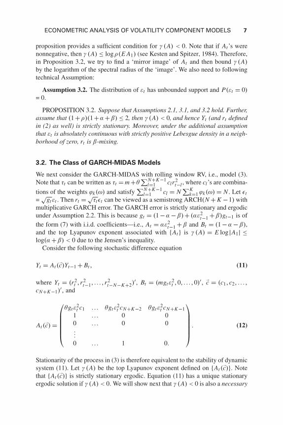
proposition provides a sufficient condition for γ (A) < 0. Note that if At ’s werenonnegative, then γ (A) ≤ logρ(E A1) (see Kesten and Spitzer, 1984). Therefore,in Proposition 3.2, we try to find a ‘mirror image’ of At and then bound γ (A)by the logarithm of the spectral radius of the ‘image’. We also need to followingtechnical Assumption:
Assumption 3.2. The distribution of εt has unbounded support and P(εt = 0)= 0.
PROPOSITION 3.2. Suppose that Assumptions 2.1, 3.1, and 3.2 hold. Further,assume that (1+ρ)(1+α +β) ≤ 2, then γ (A) < 0, and hence Yt (and rt definedin (2) as well) is strictly stationary. Moreover, under the additional assumptionthat εt is absolutely continuous with strictly positive Lebesgue density in a neigh-borhood of zero, rt is β-mixing.
3.2. The Class of GARCH-MIDAS Models
We next consider the GARCH-MIDAS with rolling window RV, i.e., model (3).Note that τt can be written as τt = m +θ
∑N+K−1l=1 clr2
t−l , where cl ’s are combina-
tions of the weights ϕk(ω) and satisfy∑N+K−1
l=1 cl = N∑K
k=1 ϕk(ω) = N . Let εt
=√
gtεt . Then rt = √τtεt can be viewed as a semistrong ARCH(N + K −1) with
multiplicative GARCH error. The GARCH error is strictly stationary and ergodicunder Assumption 2.2. This is because gt = (1 −α −β)+ (αε2
t−1 +β)gt−1 is ofthe form (7) with i.i.d. coefficients—i.e., At = αε2
t−1 +β and Bt = (1 −α −β),and the top Lyapunov exponent associated with {At } is γ (A) = E log |A1| ≤log(α +β) < 0 due to the Jensen’s inequality.
Consider the following stochastic difference equation
Yt = At (�c)Yt−1 + Bt , (11)
where Yt = (r2t ,r2
t−1, . . . ,r2t−N−K+2)
′, Bt = (mgtε2t ,0, . . . ,0)′, �c = (c1,c2, . . . ,
cN+K−1)′, and
At (�c) =
⎛⎜⎜⎜⎜⎜⎝
θgtε2t c1 . . . θgtε
2t cN+K−2 θgtε
2t cN+K−1
1 . . . 0 00 . . . 0 0...0 . . . 1 0.
⎞⎟⎟⎟⎟⎟⎠ . (12)
Stationarity of the process in (3) is therefore equivalent to the stability of dynamicsystem (11). Let γ (A) be the top Lyapunov exponent defined on {At (�c)}. Notethat {At (�c)} is strictly stationary ergodic. Equation (11) has a unique stationaryergodic solution if γ (A) < 0. We will show next that γ (A) < 0 is also a necessary
8 FANGFANG WANG AND ERIC GHYSELS
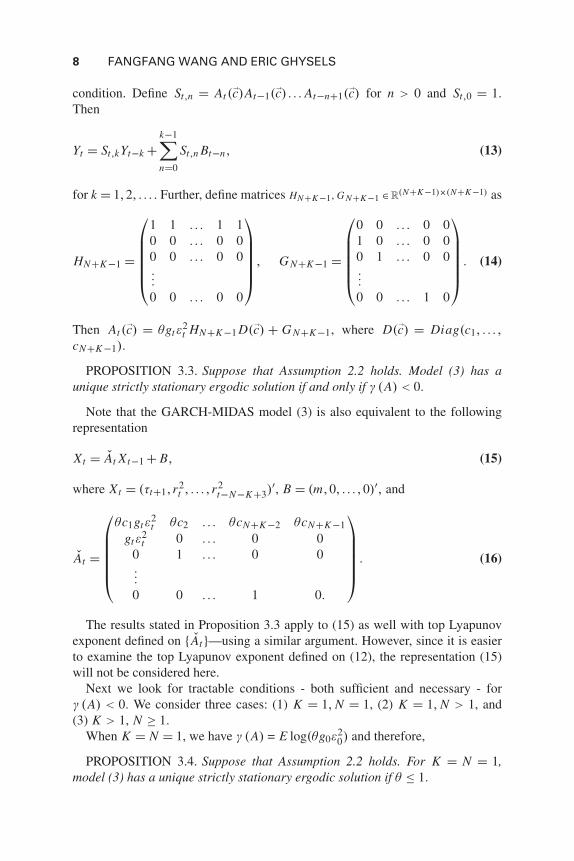
condition. Define St,n = At (�c)At−1(�c) . . . At−n+1(�c) for n > 0 and St,0 = 1.Then
Yt = St,kYt−k +k−1∑n=0
St,n Bt−n, (13)
for k = 1,2, . . . . Further, define matrices HN+K−1, G N+K−1 ∈R(N+K−1)×(N+K−1) as
HN+K−1 =
⎛⎜⎜⎜⎜⎜⎝
1 1 . . . 1 10 0 . . . 0 00 0 . . . 0 0...0 0 . . . 0 0
⎞⎟⎟⎟⎟⎟⎠ , G N+K−1 =
⎛⎜⎜⎜⎜⎜⎝
0 0 . . . 0 01 0 . . . 0 00 1 . . . 0 0...0 0 . . . 1 0
⎞⎟⎟⎟⎟⎟⎠ . (14)
Then At (�c) = θgtε2t HN+K−1 D(�c) + G N+K−1, where D(�c) = Diag(c1, . . . ,
cN+K−1).
PROPOSITION 3.3. Suppose that Assumption 2.2 holds. Model (3) has aunique strictly stationary ergodic solution if and only if γ (A) < 0.
Note that the GARCH-MIDAS model (3) is also equivalent to the followingrepresentation
Xt = At Xt−1 + B, (15)
where Xt = (τt+1,r2t , . . . ,r2
t−N−K+3)′, B = (m,0, . . . ,0)′, and
At =
⎛⎜⎜⎜⎜⎜⎝
θc1gtε2t θc2 . . . θcN+K−2 θcN+K−1
gtε2t 0 . . . 0 0
0 1 . . . 0 0...0 0 . . . 1 0.
⎞⎟⎟⎟⎟⎟⎠ . (16)
The results stated in Proposition 3.3 apply to (15) as well with top Lyapunovexponent defined on {At }—using a similar argument. However, since it is easierto examine the top Lyapunov exponent defined on (12), the representation (15)will not be considered here.
Next we look for tractable conditions - both sufficient and necessary - forγ (A) < 0. We consider three cases: (1) K = 1, N = 1, (2) K = 1, N > 1, and(3) K > 1, N ≥ 1.
When K = N = 1, we have γ (A) = E log(θg0ε20) and therefore,
PROPOSITION 3.4. Suppose that Assumption 2.2 holds. For K = N = 1,model (3) has a unique strictly stationary ergodic solution if θ ≤ 1.
ECONOMETRIC ANALYSIS OF VOLATILITY COMPONENT MODELS 9
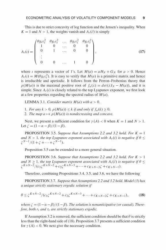
This is due to strict concavity of log function and the Jensen’s inequality. WhenK = 1 and N > 1, the weights vanish and At (�c) is simply
At (ι) =
⎛⎜⎜⎜⎜⎜⎝
θgtε2t θgtε
2t . . . θgtε
2t θgtε
2t
1 0 . . . 0 00 1 . . . 0 0...0 0 . . . 1 0
⎞⎟⎟⎟⎟⎟⎠ , (17)
where ι represents a vector of 1’s. Let M(a) = aHN + G N for a > 0. HenceAt (ι) = M(θgtε
2t ). It is easy to verify that M(a) is a primitive matrix and hence
is irreducible and aperiodic. It follows from the Perron–Frobenius theory thatρ(M(a)) is the maximal positive root of fa(λ) = det (λIN − M(a)), and it issimple. Since At (ι) is closely related to the top Lyapunov exponent, we first lookat a few properties regarding the spectral radius of M(a).
LEMMA 3.1. Consider matrix M(a) with a > 0.
1. For any k > 0, ρ(M(a)) ≤ k if and only if fa(k) ≥ 0.2. The map a → ρ(M(a)) is nondecreasing and concave.
Next, we present a sufficient condition for γ (A) < 0 when K = 1 and N > 1.Let ζ = (1−α −β)/(1−β).
PROPOSITION 3.5. Suppose that Assumptions 2.2 and 3.2 hold. For K = 1and N > 1, the top Lyapunov exponent associated with At (ι) is negative if θ ≤ζ N−1/(1+ ζ +·· ·+ ζ N−1).
Proposition 3.5 can be extended to a more general situation.
PROPOSITION 3.6. Suppose that Assumptions 2.2 and 3.2 hold. For K > 1and N ≥ 1, the top Lyapunov exponent associated with At (�c) is negative if θ ≤ζ K+N−2/(c1ζ
K+N−2 + c2ζK+N−3 +·· ·+ cK+N−2ζ + cK+N−1).
Therefore, combining Propositions 3.4, 3.5, and 3.6, we have the following
PROPOSITION 3.7. Suppose that Assumptions 2.2 and 3.2 hold. Model (3) hasa unique strictly stationary ergodic solution if
θ ≤ ζ K+N−2/(c1ζK+N−2 + c2ζ
K+N−3 +·· ·+ cK+N−2ζ + cK+N−1), (18)
where ζ = (1−α−β)/(1−β). The solution is nonanticipative (or causal). There-fore, both rt and τt are strictly stationary ergodic.
If Assumption 3.2 is removed, the sufficient condition should be that θ is strictlyless than the right-hand side of (18). Proposition 3.7 presents a sufficient conditionfor γ (A) < 0. We next give the necessary condition.
10 FANGFANG WANG AND ERIC GHYSELS
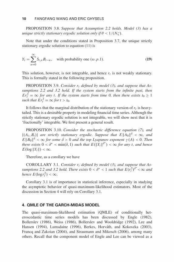
PROPOSITION 3.8. Suppose that Assumption 2.2 holds. Model (3) has aunique strictly stationary ergodic solution only if θ < 1/(Nζ ).
Note that under the conditions stated in Proposition 3.7, the unique strictlystationary ergodic solution to equation (11) is
Yt =∞∑
n=0
St,n Bt−n, with probability one (w.p.1). (19)
This solution, however, is not integrable, and hence rt is not weakly stationary.This is formally stated in the following proposition.
PROPOSITION 3.9. Consider rt defined by model (3), and suppose that As-sumptions 2.2 and 3.2 hold. If the system starts from the infinite past, thenEr2
t = ∞ for any t. If the system starts from time 0, then there exists t0 ≥ 1such that Er2
t = ∞ for t > t0.
It follows that the marginal distribution of the stationary version of rt is heavy-tailed. This is a desirable property in modeling financial time series. Although thestrictly stationary ergodic solution is not integrable, we will show next that it is‘fractionally’ integrable. We first present a general result.
PROPOSITION 3.10. Consider the stochastic difference equation (7), and{(At , Bt )} are strictly stationary ergodic. Suppose that E‖A0‖δ < ∞, andE‖B0‖δ < ∞ for some δ > 0 and the top Lyapunov exponent γ (A) < 0. Thenthere exists 0 < δ∗ < min(δ,1) such that E(‖Yt‖δ∗
) < ∞ for any t, and henceE(log‖Yt‖) < ∞.
Therefore, as a corollary we have
COROLLARY 3.1. Consider rt defined by model (3), and suppose that As-sumptions 2.2 and 3.2 hold. There exists 0 < δ∗ < 1 such that E(r2
t )δ∗<∞ and
hence E(logr2t ) < ∞.
Corollary 3.1 is of importance in statistical inference, especially in studyingthe asymptotic behavior of quasi-maximum-likelihood estimators. Most of thediscussion in Section 4 will rely on Corollary 3.1.
4. QMLE OF THE GARCH-MIDAS MODEL
The quasi-maximum-likelihood estimation (QMLE) of conditionally het-eroscedastic time series models has been discussed by Engle (1982),Bollerslev (1986), Weiss (1986), Bollerslev and Wooldridge (1992), Lee andHansen (1994), Lumsdaine (1996), Berkes, Horvath, and Kokoszka (2003),Francq and Zakoian (2004), and Straumann and Mikosch (2006), among manyothers. Recall that the component model of Engle and Lee can be viewed as a

ECONOMETRIC ANALYSIS OF VOLATILITY COMPONENT MODELS 11
GARCH (2,2). The QMLE asymptotic analysis of Engle (1982) and Bollerslev(1986) therefore straightforwardly applies.8
Unfortunately, the existing asymptotic results do not directly carry over to theGARCH-MIDAS class of models. In this section, we cover the asymptotic anal-ysis of the quasi-maximum-likelihood estimator for the GARCH-MIDAS modelwith rolling-window RV.
Let U be the parameter space which will be specified later. Define gt and τt as
gt ( ) = (1−α −β)+αr2
t−1
τt−1( )+βgt−1( ), (20)
τt ( ) = m + θ
K∑k=1
ϕk(ω)RVt−k, (21)
for = (α,β,m,θ,ω) ∈ U and t ∈Z. Suppose that 0 = (α0,β0,m0,θ0,ω0) ∈ Uis the true parameter such that
rt = √gt ( 0)τt ( 0)εt , t ∈ Z, (22)
where εt ∼ I I D(0,1) and ε2t has a nondegenerate distribution. Given a finite
record of rt : {rt ,1 ≤ t ≤ T } where T � N + K , define
gt ( ) = (1−α −β)+αr2
t−1τt−1
+β gt−1( ),
τt ( ) = m + θ∑K
k=1 ϕk(ω)RVt−k,(23)
for t = N + K +1, . . . ,T , and gN+K is an arbitrary number. The QMLE of 0 isthe minimizer of
LT ( ) = 1
T − N − K
T∑t=N+K+1
log Vt ( )+ r2t
Vt ( ), (24)
for ∈U , where Vt ( ) = gt ( )τt ( ). The estimator is denoted by T . Considera companion estimator, T , which minimizes
LT ( ) = 1
T − (N + K )
T∑t=N+K+1
log Vt ( )+ r2t
Vt ( )(25)
over ∈ U where Vt ( ) = gt ( )τt ( ). Clearly, τt ( ) = τt ( ). Although T isnot feasible, it is theoretically tractable and T − T = op(1/
√T ) (see the proof
of Proposition 4.2).The properties of T and T are closely related to the choice of parameter
space U . Suppose that the parameter ω is of dimension d, i.e., ω = (ω1, . . . ,ωd)′.The weights are parameterized by ω. We rule out the degenerate case that ϕk ≡ 0for some k ∈ {1,2, . . . , K }. We also assume the weights ϕk(ω) satisfy the follow-ing conditions.
12 FANGFANG WANG AND ERIC GHYSELS
Assumption 4.1. There exists an open set � ⊂ Rd such that for k ∈
{1,2, . . . , K − 1} and ω ∈ �, ϕk(ω) ≥ 0, ϕ1(ω) + ·· · + ϕK−1(ω) ≤ 1 and thesecond-order partial derivative ∂2ϕk(ω)/∂ω2
j exists and is continuous on �, and
the (K − 1)-by-d matrix(∂ϕk(ω)/∂ωj
)(K−1)×d has rank greater than or equal
to d.
Remark 4.1. Because ϕK = 1 − ϕ1 − ·· · − ϕK−1, under Assumption 4.1 wehave ϕk(ω) = ϕk(ω0) if and only if ω = ω0 for all k. For easy exposition werestrict our attention to the case where ω is a scalar for the rest of analysis, i.e.,d = 1.
Note that Proposition 3.7 holds when β = 0 and/or θ = 0, and θ = 0 as it yieldsthe regular GARCH(1,1). However, for estimation purpose we need to excludesuch cases as it makes the weighting function unidentifiable. We will thereforerequire the true parameter θ0 > 0. Define
U1 ={ = (α,β,m,θ,ω)′ ∈ R5 : α > 0,β ≥ 0,α +β < 1,m > 0,
0 < θ ≤ ζ K+N−2
c1ζ K+N−2 + c2ζ K+N−3 +·· ·+ cK+N−2ζ + cK+N−1,ω ∈ �
},
(26)
where ζ = (1−α −β)/(1−β). Moreover, define
U2 = { = (α,β,m,θ,ω)′ ∈ R5 : α ≥ 0,β ≥ 0,α +β < 1,m > 0,θ > 0,ω ∈ �}.(27)
Clearly, U2 contains U1. The process r2t is strictly stationary ergodic, if 0 ∈
U1 and Assumption 3.2 holds. The parameter space will satisfy the followingassumption:
Assumption 4.2. The parameter space U is a compact subset of U2. The trueparameter 0 is in both U and U1, i.e., 0 ∈ U ∩U1.
Consider lt ( ) = log Vt ( )+ r2t /Vt ( ).
LEMMA 4.1. Under Assumptions 3.2, 4.2, and 4.1, E sup ∈U | log(gt ( ))| andE sup ∈U | log(τt ( ))| are finite, and hence E sup ∈U l−t ( ) < ∞.9
It follows that under Assumption 4.2, Elt ( ) is well defined for ∈ U . More-over, E |lt ( 0)| < ∞ but E sup ∈U |lt ( )| = ∞. Next we will show that 0 isidentifiably unique. In other words, Elt ( ) is uniquely minimized at 0.
LEMMA 4.2. Under Assumptions 3.2, 4.2, and 4.1, Elt ( ) > Elt ( 0) for ∈ U and �= 0.
ECONOMETRIC ANALYSIS OF VOLATILITY COMPONENT MODELS 13
Because Elt ( ) may not be finite for ∈ U , the uniform Strong Law of LargeNumbers (SLLN) does not apply. We need the following lemma for the proof ofstrong consistency of T and T .
LEMMA 4.3. Suppose that Assumptions 3.2, 4.2, and 4.1 hold. For any com-pact set C ⊂ U , then liminfT →∞ inf ∈C LT ( ) ≥ inf ∈C Elt ( ) almost surely(a.s.).
The proof is skipped. The reader is referred to Lemma 3.11 of Pfanzagl (1969).The next lemma shows that the asymptotic property of T is independent of thestarting value.
LEMMA 4.4. Under Assumptions 3.2 and 4.2,
limT →∞ sup
∈U|LT ( )− LT ( )| = 0 almost surely. (28)
Therefore, we have the following
PROPOSITION 4.1. Under Assumptions 3.2, 4.2, and 4.1, T and T con-verge to 0 almost surely.
Remark 4.2. Note that if ϕk(ω) > 0 for ω ∈ � and k = 1,2, . . . , K , then
τt ( 0)
τt= m0
τt+
K∑k=1
θ0ϕk(ω0)RVt−k
τt≤ m0
m+
K∑k=1
θ0ϕk(ω0)
θϕk(ω). (29)
We would have E sup ∈U V −1t r2
t < ∞ and E sup ∈U |lt ( )| < ∞. Therefore,the proof of Proposition 4.1 will be a direct application of the uniform SLLN (see,for instance, Theorem 3.3 of Gallant and White, 1988).
Further, we will show that T is also asymptotic normal, with an additional as-sumption. Let ϕ = (ϕ1, . . . ,ϕK−1) and V = {(x1, . . . , xK−1) : x1 > 0, . . . , xK−1 >0, x1 +·· ·+ xK−1 < 1}.
Assumption 4.3. E(ε4t ) < ∞. The true parameter 0 is an interior point of U ,
i.e., 0 ∈ U0, and ϕ(ω0) ∈ V .
By continuity of ϕk , there exists an open ball Oω0 such that ω0 ∈ Oω0 ⊂Oω0 ⊂ � and ϕ(Oω0) ⊂ V . Therefore, one can always find a compact set Asuch that 0 ∈ A ⊂ U0 and for = (α,β,m,θ,ω)′ ∈ A, ϕ(ω) ∈ V . Define
�( ) = E(
V −2t ( )∇Vt ( )∇Vt ( )′
)for ∈A.10
LEMMA 4.5. Suppose that Assumptions 3.2, 4.2, 4.1, and 4.3 hold. Then
1. �( ) exists and it is positive definite at 0.2.
√T ∇LT ( 0) =⇒ N (0, (Eε4
t −1)�( 0)).
14 FANGFANG WANG AND ERIC GHYSELS
3. Let B( 0,1/n) = { ∈ R5 : ‖ − 0‖ < 1/n}.limsup
n→∞lim
T →∞ sup ∈B( 0,1/n)∩A
‖H(LT )( )−�( 0)‖ = 0 a.s. (30)
4. limT →∞√
T sup ∈A ‖∇LT ( )−∇ LT ( )‖ = 0 in probability.
Lemma 4.5 allows us to establish the asymptotic normality of T .
PROPOSITION 4.2. Under Assumptions 3.2, 4.2, 4.1, and 4.3,
√T ( T − 0) =⇒ N (0, (Eε4
t −1)�( 0)−1).
Remark 4.3. Note that gt ( 0) = (1−α0 −β0)+ (α0ε2t−1 +β0)gt−1( 0), and
τt ( 0) = m0 +θ0∑K
k=1 ϕk(ω0)RVt−k . Denote by ∂α,∂β,∂m,∂θ , and ∂ω the partialderivatives with respect to α,β,m,θ , and ω, respectively. We have ∂m gt ( 0) =∂θ gt ( 0) = ∂ωgt ( 0) = ∂ατt ( 0) = ∂βτt ( 0) = 0, and thus
∇gt ( 0) = (∂αgt ( 0),∂βgt ( 0),0,0,0)′,∇τt ( 0) = (0,0,∂mτt ( 0),∂θ τt ( 0),∂ωτt ( 0))
′.
Note also that
V −2t ( 0)∇Vt ( 0)∇Vt ( 0)
′
= ∇gt ( 0)∇gt ( 0)′
gt ( 0)2+ ∇τt ( 0)∇τt ( 0)
′
τt ( 0)2+ ∇τt ( 0)∇gt ( 0)
′
τt ( 0)gt ( 0)
+ ∇gt ( 0)∇τt ( 0)′
τt ( 0)gt ( 0).
It follows that �( 0) = E(
V −2t ( 0)∇Vt ( 0)∇Vt ( 0)
′)
is a block di-
agonal matrix, and �( 0) = Diag(J1, J2) where J1 = E(
g−2t ( 0)dgt dg′
t
)and J2 = E
(τ−2
t ( 0)dτt dτ ′t
), and dgt = (∂αgt ( 0),∂βgt ( 0))
′ and dτt =(∂mτt ( 0),∂θ τt ( 0),∂ωτt ( 0))
′. The asymptotic variance becomes (Eε4t − 1)
Diag(J−11 , J−1
2 ). For the MLE T = (αT , βT , mT , θT , ωT )′, (αT , βT )′, and(mT , θT , ωT )′ are asymptotically independent.
Remark 4.4. It should be noted that the results of QMLE can be easilyextended to ω being multidimensional. The proofs of Lemmas 4.1–4.4 andProposition 4.1 apply to a vector ω without modification. For Lemma 4.5 andProposition 4.2, we just need to replace the (partial) derivative with respect to ωby the partial derivative with respect to each component of ω, and the discussionfollows directly.
ECONOMETRIC ANALYSIS OF VOLATILITY COMPONENT MODELS 15
5. CONCLUSION
This paper revisits the component models from a probabilistic and statistical per-spective. Stationarity of two models is investigated: the component model ofEngle and Lee (1999), and the GARCH-MIDAS models of Engle, Ghysels, andSohn (2013). By examining the associated top Lyapunov exponents, we presentexplicit conditions on the space of parameters—both sufficient and necessary—for stationarity and ergodicity. This is necessary, because it allows one to easilytrack stationarity of the underlying process with given parameters and to man-age model inference. A by-product regarding the analysis of Lyapunov exponentsis that γ (A) < 0 is also a necessary condition for stationarity and ergodicity ofModel (3).
We also show that the GARCH-MIDAS model has fat-tailed marginal dis-tribution, a desirable property in modeling financial time series. We then studysampling behavior of the quasi-maximum-likelihood estimator of the model. Theconsistency and asymptotic normality of the QMLE are established.
NOTES
1. Applications of Spline-GARCH and GARCH-MIDAS include Baele, Bekaert, and Inghelbrecht(2010), Bauwens, Hafner, and Pierret (2013), Chauvet, Senyuz, and Yoldas (2010), Chen, Choudhry,and Wu (2013), Dorion (2010), Golosnoy, Gribisch, and Liesenfeld (2012), Hafner and Linton (2010),Asgharian, Hou, and Javed (2013), Maheu and McCurdy (2007), and Rangel (2011), among others.
2. We use generic parameter settings across all the models to avoid a proliferation of parameternotation. Therefore, it is important to note that the parameters in the models (2) and (3) are not related.For example, the ω in (2) is different from the ω appearing in (3).
3. The stationarity of Yt of the form (7) has been studied extensively in the literature, see forinstance, Pham (1985, 1986), Brandt (1986), Bougerol (1987), Meyn and Caines (1991), Bougeroland Picard (1992a, 1992b), and Glasserman and Yao (1995), among others.
4. Model (7) is said to be irreducible if no proper affine subspaceH ∈Rd exists such that {At y +Bt : y ∈H} ⊆H. For details on irreducibility, the reader is referred to for example Meyn and Caines(1991), Bougerol and Picard (1992b), and Kristensen (2009).
5. It should be noted that the Jacobian determinant of the map from (ω,α,β,φ,ρ) to(α0,α1,α2,β1,β2) is −(1 − α − β)(α + β − ρ)2, and it is not zero under Assumption 2.1. There-fore, (ω,α,β,φ,ρ) can be identified from (α0,α1,α2,β1,β2).
6. See Engle and Lee (1999, p. 479).7. A random variable X is said to have a continuous component at 0, if there exists a function
f > 0 and a constant δ > 0 such that P(X ∈A) ≥ ∫A∩(−δ,δ) f (x)dx for any Borel setA⊆ R.
8. See the discussion in Engle and Lee (1999) for details.9. Where l−t ( ) = max(−lt ( ),0).
10. We use ∇ to denote the vector differential operator so that ∇ f is the gradient (column vector)of scalar function f , and H( f ) the Hessian matrix of f .
11. This notation is used only in the proof of Lemma 4.2. For a set U , U0 represents the interiorof U .
REFERENCES
Adrian, T. & J. Rosenberg (2008) Stock returns and volatility: Pricing the short-run and long-runcomponents of market risk. Journal of Finance 63, 2997–3030.
16 FANGFANG WANG AND ERIC GHYSELS
Asgharian, H., A. J. Hou, & F. Javed (2013) The Importance of the Macroeconomic Variables inForecasting Stock Return Variance: A GARCH-MIDAS Approach, Journal of Forecasting, 32(7),600–612.
Alizadeh, S., M. Brandt, & F. Diebold (2002) Range-based estimation of stochastic volatility models.Journal of Finance 57, 1047–1091.
Andreou, E. & E. Ghysels (2002) Detecting multiple breaks in financial market volatility dynamics.Journal of Applied Econometrics 17, 579–600.
Baele, L., G. Bekaert, & K. Inghelbrecht (2010) The determinants of stock and bond return comove-ments. Review of Financial Studies 23, 2374–2428.
Basrak, B., R. Davis, & T. Mikosch (2001) Sample ACF of multivariate stochastic recurrence equa-tions with application to GARCH. Preprint, Available at www. math. ku. dk/mikosch.
Bauwens, L., C. M. Hafner, & D. Pierret (2013) Multivariate volatility modeling of electricity futures,Journal of Applied Econometrics, 28(5), 743–761.
Berkes, I., E. Gombay, L. Horvath, & P. Kokoszka (2004) Sequential change-point detection inGARCH(p,q) models. Econometric Theory 20, 1140–1167.
Berkes, I., L. Horvath, & P. Kokoszka (2003) GARCH processes: Structure and estimation. Bernoulli9, 201–227.
Bollerslev, T. (1986) Generalized autoregressive conditional heteroskedasticity. Journal of Economet-rics 31, 307–327.
Bollerslev, T. & J. Wooldridge (1992) Quasi-maximum likelihood estimation and inference in dynamicmodels with time-varying covariances. Econometric Reviews 11, 143–172.
Bougerol, P. (1987) Tightness of products of random matrices and stability of linear stochastic sys-tems. Annals of Probability 15, 40–74.
Bougerol, P. & N. Picard (1992a) Stationarity of GARCH processes and of some nonnegative timeseries. Journal of Econometrics 52, 115–127.
Bougerol, P. & N. Picard (1992b) Strict stationarity of generalized autoregressive processes. Annalsof Probability 20, 1714–1730.
Brandt, A. (1986) The stochastic equation Yn+1 = AnYn + Bn with stationary coefficients. Advancesin Applied Probability 18, 211–220.
Carrasco, M. & X. Chen (2002) Mixing and moment properties of various GARCH and stochasticvolatility models. Econometric Theory 18, 17–39.
Chauvet, M., Z. Senyuz, & E. Yoldas (2010) What Does Realized Volatility Tell Us About Macroeco-nomic Fluctuations? Discussion paper, Working paper, University of California, Riverside.
Chen, M. & H. An (1998) A note on the stationarity and the existence of moments of the GARCHmodel. Statistica Sinica 8, 505–510.
Chen, W.-P., T. Choudhry, & C.-C. Wu (2013) The extreme value in crude oil and US dollar markets.Journal of International Money and Finance 36, 191–210.
Chen, J. & A. Gupta (1997) Testing and locating variance changepoints with application to stockprices. Journal of the American Statistical Association 92, 739–747.
Chernov, M., A. Gallant, E. Ghysels, & G. Tauchen (2003) Alternative models for stock price dynam-ics. Journal of Econometrics 116, 225–257.
Cohen, J. & C. Newman (1984) The stability of large random matrices and their products. Annalsof Probability 12, 283–310.
Dahlhaus, R. & S. Rao (2006) Statistical inference for time-varying ARCH processes. Annals of Statis-tics 34, 1075–1114.
Ding, Z. & C. Granger (1996) Modeling volatility persistence of speculative returns: A new approach.Journal of Econometrics 73, 185–215.
Dorion, C. (2010) Business Conditions, Market Volatility and Option Prices. Discussion paper, HECMontreal Working paper.
Duan, J. (1997) Augmented GARCH (p,q) process and its diffusion limit. Journal of Econometrics79, 97–127.
Engle, R. (1982) Autoregressive conditional heteroscedasticity with estimates of the variance ofUnited Kingdom inflation. Econometrica 50, 987–1007.
ECONOMETRIC ANALYSIS OF VOLATILITY COMPONENT MODELS 17
Engle, R. & G. Lee (1999) A long-run and short-run component model of stock return volatility. InR. Engle & H. White (eds.), Cointegration, Causality, and Forecasting: A Festschrift in Honourof Clive WJ Granger, pp. 475–497. Oxford University Press.
Engle, R. & J. Rangel (2008) The spline-GARCH model for low-frequency volatility and its globalmacroeconomic causes. Review of Financial Studies 21, 1187–1222.
Engle, R. F., E. Ghysels, & B. Sohn (2013) Stock market volatility and macroeconomic fundamentals,Review of Economics and Statistics, 95(3), 776–797.
Francq, C. & J. Zakoian (2004) Maximum likelihood estimation of pure GARCH and ARMA-GARCH processes. Bernoulli 10, 605–637.
Francq, C. & J. Zakoian (2006) Mixing properties of a general class of GARCH (1, 1) models withoutmoment assumptions on the observed process. Econometric Theory 22, 815–834.
Francq, C. & J. Zakoian (2009) A tour in the asymptotic theory of GARCH estimation. Handbookof Financial Time Series, pp. 85–111. Springer.
Francq, C. & J. Zakoian (2010) GARCH Models: Structure, Statistical Inference and Financial Appli-cations. Wiley.
Furstenberg, H. (1963) Noncommuting random products. Transactions of the American MathematicalSociety 108, 377–428.
Furstenberg, H. & H. Kesten (1960) Products of random matrices. Annals of Mathematical Statistics31, 457–469.
Gallant, A. & H. White (1988) A Unified Theory of Estimation and Inference for Nonlinear DynamicModels. Basil Blackwell.
Ghysels, E. (2013) Matlab toolbox for MIDAS regressions. Available at http://www.unc.edu/∼eghysels.
Ghysels, E., P. Santa-Clara, & R. Valkanov (2004) The MIDAS Touch: Mixed Data Sampling Regres-sion Models. CIRANO.
Ghysels, E., P. Santa-Clara, & R. Valkanov (2005) There is a risk-return trade-off after all. Journalof Financial Economics 76, 509–548.
Ghysels, E., P. Santa-Clara, & R. Valkanov (2006) Predicting volatility: Getting the most out of returndata sampled at different frequencies. Journal of Econometrics 131, 59–95.
Ghysels, E., A. Sinko, & R. Valkanov (2006) MIDAS regressions: Further results and new directions.Econometric Reviews 26, 53–90.
Glasserman, P. & D. Yao (1995) Stochastic vector difference equations with stationary coefficients.Journal of Applied Probability 32, 851–866.
Goldsheid, I. (1991) Lyapunov exponents and asymptotic behaviour of the product of random matri-ces. Lyapunov Exponents, pp. 23–37. Springer.
Golosnoy, V., B. Gribisch, & R. Liesenfeld (2012) The conditional autoregressive Wishart model formultivariate stock market volatility. Journal of Econometrics 167, 211–223.
Hafner, C. & O. Linton (2010) Efficient estimation of a multivariate multiplicative volatility model.Journal of Econometrics 159, 55–73.
He, C. & T. Terasvirta (1999) Properties of moments of a family of GARCH processes. Journalof Econometrics 92, 173–192.
Horvath, L., P. Kokoszka, & G. Teyssiere (2001) Empirical process of the squared residuals of anARCH sequence. Annals of Statistics 29, 445–469.
Horvath, L., P. Kokoszka, & A. Zhang (2006) Monitoring constancy of variance in conditionally het-eroskedastic time series. Econometric Theory 22, 373–402.
Inclan, C. & G. Tiao (1994) Use of cumulative sums of squares for retrospective detection of changesof variance. Journal of the American Statistical Association 89, 913–923.
Kesten, H. & F. Spitzer (1984) Convergence in distribution of products of random matrices. Probabil-ity Theory and Related Fields 67, 363–386.
Kingman, J. (1973) Subadditive ergodic theory. Annals of Probability 1, 883–899.Kokoszka, P. & R. Leipus (2000) Change-point estimation in ARCH models. Bernoulli 6, 513–540.Kristensen, D. (2009) On stationarity and ergodicity of the bilinear model with applications to
GARCH models. Journal of Time Series Analysis 30, 125–144.
18 FANGFANG WANG AND ERIC GHYSELS
Kulperger, R. & H. Yu (2005) High moment partial sum processes of residuals in GARCH models andtheir applications. Annals of Statistics 33, 2395–2422.
Lee, S. & B. Hansen (1994) Asymptotic theory for the GARCH (1, 1) quasi-maximum likelihoodestimator. Econometric Theory 10, 29–29.
Lindner, A. (2009) Stationarity, mixing, distributional properties and moments of GARCH (p, q)–processes. Handbook of Financial Time Series, pp. 43–69. Springer.
Lu, Z. & R. Smith (1997) Estimating local Lyapunov exponents. Fields Institute Communications 11,135–151.
Lumsdaine, R. (1996) Consistency and asymptotic normality of the quasi-maximum likelihood es-timator in IGARCH (1, 1) and covariance stationary GARCH (1, 1) models. Econometrica 64,575–596.
Maheu, J. & T. McCurdy (2007) Components of market risk and return. Journal of Financial Econo-metrics 5, 560–590.
Meitz, M. & P. Saikkonen (2008) Ergodicity, mixing, and existence of moments of a classof Markov models with applications to GARCH and ACD models. Econometric Theory 24,1291–1320.
Merton, R.C. (1980) On estimating the expected return on the market: An exploratory investigation.Journal of Financial Economics 8, 323–361.
Meyn, S.P. & P.E. Caines (1991) Asymptotic behavior of stochastic systems possessing Markovianrealizations. SIAM Journal on Control and Optimization 29, 535–561.
Mokkadem, A. (1990) Proprietes de melange des processus autoregressifs polynomiaux. Annales del’Institut Henri Poincare (B) Probabilites et statistiques 26, 219–260.
Nelson, D. (1990) Stationarity and persistence in the GARCH (l, l) model. Econometric Theory 6,318–334.
Newman, C. (1986) The distribution of Lyapunov exponents: Exact results for random matrices. Com-munications in Mathematical Physics 103, 121–126.
Peres, Y. (1992) Domains of analytic continuation for the top Lyapunov exponent. Annales de l’InstitutHenri Poincare (B) Probabilites et statistiques 28, 131–148.
Pfanzagl, J. (1969) On the measurability and consistency of minimum contrast estimates. Metrika 14,249–272.
Pham, D. (1985) Bilinear markovian representation and bilinear models. Stochastic Processes andtheir Applications 20, 295–306.
Pham, D. (1986) The mixing property of bilinear and generalised random coefficient autoregressivemodels. Stochastic Processes and their Applications 23, 291–300.
Rangel, J. (2011) Macroeconomic news, announcements, and stock market jump intensity dynamics.Journal of Banking and Finance 35, 1263–1276.
Schwert, G.W. (1989) Why does stock market volatility change over time? Journal of Finance 44,1207–1239.
Seneta, E. (1981) Non-negative Matrices and Markov Chains. Springer Verlag.Straumann, D. & T. Mikosch (2006) Quasi-maximum-likelihood estimation in conditionally het-
eroscedastic time series: A stochastic recurrence equations approach. Annals of Statistics 34,2449–2495.
Vanneste, J. (2010) Estimating generalized Lyapunov exponents for products of random matrices.Physical Review E 81, 036701.
Weiss, A. (1986) Asymptotic theory for ARCH models: Estimation and testing. Econometric Theory2, 107–131.
Whang, Y. & O. Linton (1999) The asymptotic distribution of nonparametric estimates of the Lya-punov exponent for stochastic time series. Journal of Econometrics 91, 1–42.
Yao, J. (2001) On square-integrability of an AR process with Markov switching. Statistics and Prob-ability Letters 52, 265–270.
ECONOMETRIC ANALYSIS OF VOLATILITY COMPONENT MODELS 19
APPENDIX
Proof of Proposition 3.1. Note that (Z) has roots outside the unit circle (see Engleand Lee, 1999). Moreover, since
(−α1/α2) = 1+β1α1/α2 −β2α21/α2
2 = − 1
α22
(ρ −α −β)2αφ �= 0,
if and only if ρ − α − β and α and φ are not 0, then (Z) and �(Z) have no commonroots, and hence Yt is irreducible. n
Proof of Proposition 3.2. We only need to show γ (A) < 0. Let
Mt = A(ε2t )A(ε2
t−1) . . . A(ε21), Mt = A(ε2
t ) A(ε2t−1) . . . A(ε2
1),
where
A(x) =⎛⎝β1 +α1x −β2 −α2
1 0 0x 0 0
⎞⎠ . (A.1)
Then E A(ε2t ) = A(1). By induction ‖Mt‖ ≤ ‖Mt‖ for any t. Note that A(ε2
t ) is notbounded almost surely and i.i.d. We then have limt→∞ 1
t log‖Mt‖ < log(ρ( A(1))) (seeKesten and Spitzer, 1984, Thm. 2). Because
ρ( A(1)) = α +β +ρ +√
(α +β +ρ)2 +4(α +β)ρ
2,
ρ( A(1)) ≤ 1 if and only if (1+ρ)(1+α +β) ≤ 2.Note that the characteristic function of A(0) is det (λI3 − A(0)) = λ(λ2 − β1λ − β2).
The spectral radius of A(0) is therefore less than 1. Define V (y) = |y1|+a|y2|+a|y3| fory = (y1, y2, y3)
′ ∈ R3, where a = (1 − (α1 +β1))/4 > 0. Let π = (1 +α1 +β1)/2 < 1,and B > 0 is such that (α0 +1)/B < 1−π. It is easy to verify that E[V (Yt )|Yt−1] ≤ α0 +πV (Yt−1). Define K = {k ∈R3 : V (k) ≤ B}. E[V (Yt )|Yt−1 = y] is bounded for y ∈ K . OnK c, E[V (Yt )|Yt−1 = y] ≤ α0 +πV (y) ≤ ((α0 +1)/B +π)V (y)−1. Under the additionalassumption that εt is absolutely continuous with strictly positive Lebesgue density in aneighborhood of zero, Yt is geometrically ergodic and hence rt is β-mixing, which followsfrom Mokkadem (1990) (or Theorem 1 of Carrasco and Chen, 2002; Theorem 8 of Lindner,2009). n
Proof of Proposition 3.3. Note that 1 ≤ ‖A0(�c)‖ ≤ θg0ε20‖HN+K−1 D(�c)‖+‖G N+K−1‖ ≤
Nθg0ε20 +1. We have E(log‖A0(�c)‖) ≤ E log(Nθg0ε2
0 +1) ≤ E(Nθg0ε20) < ∞.
Sufficiency follows from Theorem 3.1 of Glasserman and Yao (1995) (see also Bougeroland Picard, 1992b). The necessity is done through an argument similar to the proof ofTheorem 1.3 of Bougerol and Picard (1992a).
Suppose that (11) has a unique strictly stationary ergodic solution. Let t = 0 in (13).Since
∑k−1n=0 S0,n B−n ≤ Y0 almost surely for any k, then limn→∞ S0,n B−n = 0 almost
surely. In other words,
limn→∞ε2−n S0,ne1 = 0 almost surely,
20 FANGFANG WANG AND ERIC GHYSELS
where {e1,e2, . . . ,eN+K−1} is the canonical basis of RN+K−1. Note that for i =1,2, . . . , N + K −2,
S0,nei = S0,n−1(θε2−n+1 HN+K−1 D(�c)+ G N+K−1)ei
= θci ε2−n+1S0,n−1e1 + S0,n−1ei+1,
S0,neN+K−1 = θcN+K−1ε2−n+1S0,n−1e1.
Therefore, limn→∞ S0,nei = 0 almost surely for any i , and hence limn→∞ S0,n = 0 almostsurely. It follows from Lemma 3.4 of Bougerol and Picard (1992b) that γ (A) < 0. n
Proof of Lemma 3.1. 1. Note that fa(λ) = λN −aλN−1 −aλN−2 −·· ·−aλ2 −aλ−a.For |λ| > k,
| fa(λ)| ≥ |λN |(1− a
|λ| − a
|λ2| − · · ·− a
|λN | )
> k N (1− a
k− a
k2−·· ·− a
k N) = f (k).
Note that ρ(M(a)) is the largest positive root of fa(λ). Therefore, ρ(M(a)) ≤ k if andonly if fa(k) ≥ 0.
2. Note that ρ(M(a)) is the maximal positive root of f (λ) = det (λI − M(a)). It issimple and ρ(M(a)) ≥ |λ| for each root λ of f (λ) = 0. For easy exposition, we simplywrite ρ(M(a)) as λ. Since f (λ) = λN −aλN−1 −aλN−2 −·· ·−aλ2 −aλ−a = 0,
a = λN
λN−1 +λN−2 +·· ·+λ2 +λ+1= λ−1+ g(λ), (A.2)
where g(λ) = 1h(λ) and h(λ) = λN−1 +λN−2 +·· ·+λ2 +λ+ 1. Note that λ is a smooth
function of a. To prove λ is a concave function of a is equivalent to show that d2λ(a)da2 < 0.
On one hand, taking derivative on both sides of (A.2) with respect to a, we have 1 =(1 + g
′)λ
′, where g
′ = dg(λ)dλ and λ
′ = dλ(a)da . Furthermore, 0 = (1 + g
′)λ
′′ + g′′(λ
′)2,
where g′′ = d2g(λ)
dλ2 and λ′′ = d2λ(a)
da2 . On the other hand, write f (λ) = 0 as F(λ,a) = 0. Byimplicit function theorem,
λ′ = − Fa
Fλ,
where Fa = ∂ F∂a = −h(λ) < 0 and Fλ > 0 (since λ is the largest root of f and f goes to
∞ as λ goes to ∞ for fixed a). Hence λ′> 0 and 1+ g
′> 0.
To show λ′′
< 0, it is sufficient to show that g′′ = 2(h
′(λ))2−h(λ)h
′′(λ)
h3(λ)> 0 or � =
2(h′(λ))2 −h(λ)h
′′(λ) > 0, where h
′ = dh(λ)dλ and h
′′ = d2h(λ)dλ2 . Note that
h(λ) = λN −1
λ−1,
h′(λ) = NλN−1
λ−1− λN −1
(λ−1)2,
h′′(λ) = N (N −1)λN−2
λ−1− 2NλN−1
(λ−1)2+ 2(λN −1)
(λ−1)3.
ECONOMETRIC ANALYSIS OF VOLATILITY COMPONENT MODELS 21
Therefore,
� = NλN−2[(N −1)λN+1 − (N +1)λN + (N +1)λ− (N −1)]
(λ−1)3. (A.3)
Define
D(λ) = (N −1)λN+1 − (N +1)λN + (N +1)λ− (N −1).
Then D′(λ)
.= d D(λ)dλ = (N − 1)(N + 1)λN − (N + 1)NλN−1 + (N + 1) and D
′′(λ)
.=d2 D(λ)
dλ2 = (N −1)N (N +1)λN−2(λ−1). Note that D(1) = D′(1) = D
′′(1) = 0 and D
′′<
0 for 0 < λ < 1, while on λ > 1, D′′
> 0. It implies that D′> 0 except λ = 1. Going one
step further, we have D > 0 on λ > 1 and D < 0 on 0 < λ < 1, which means � > 0 on bothλ > 1 and 0 < λ < 1. By continuity, � > 0 for λ > 0. It finishes the proof. n
Proof of Proposition 3.5. Let At = At (ι). Note that 1 ≤ ‖A0‖ ≤ θg0ε20‖H‖+‖G‖ =
θg0ε20 +1, and hence E(log‖A0‖) ≤ E log(θg0ε2
0 +1) ≤ Eθg0ε20 < ∞.
Note that At = gt (θε2t H + 1
gtG) ≤ gt (θε2
t H + 1ζ G). Let At = θε2
t H + 1ζ G. At , At are
nonnegative. We then have
‖At At−1 . . . A0‖ ≤ gt gt−1 . . .g0‖ At At−1 . . . A0‖.It follows that
γ (A) ≤ E log g0 + limt
1
1+ tE log ‖ At At−1 . . . A0‖ ≤ γ ,
where γ is the top Lyapunov exponent associated with the sequence {At , t ∈Z}. Since At ’sare i.i.d. and irreducible and ε has unbounded support, then γ < 0 if ρ[E( A0)] ≤ 1 (seeKesten and Spitzer, 1984, Thm. 2). Note that E( A0) = 1
ζ M(θζ ) and
ρ[E( A0)] ≤ 1 ⇐⇒ ρ[M(θζ )] ≤ ζ ⇐⇒ fθζ (ζ ) = det (ζ I − M(θζ )) ≥ 0
by Lemma 3.1. fθζ (ζ ) ≥ 0 if θ ≤ ζ N−1/(1+ ζ +·· ·+ ζ N−1). The proof is complete. n
Proof of Proposition 3.6. Note that At (�c) = θgtε2t HN+K−1 D(�c)+ G N+K−1, where
D(�c) = Diag(c1, . . . ,cN+K−1). 1 ≤ ‖A0(�c)‖ ≤ θg0ε20‖HN+K−1 D(�c)‖+‖G N+K−1‖ ≤
Nθg0ε20 +1. Hence E(log‖A0(�c)‖) ≤ E log(Nθg0ε2
0 +1) ≤ E(Nθg0ε20) < ∞.
Note that At (�c) ≤ gt (θε2t HN+K−1 D(�c)+ 1
ζ G N+K−1). Similar to the discussion in theproof of Proposition 3.5, we have γ (A) < 0 if ρ(θζ HN+K−1 D(�c)+ G N+K−1) ≤ ζ. Letf (λ) = det(λIN+K−1 − θζ HN+K−1 D(�c)− G N+K−1). Note that
f (λ) = λN+K−1 − θζc1λN+K−2 − θζc2λN+K−3 −·· ·− θζcN+K−2λ− θζcN+K−1.
The matrix θζ HN+K−1 D(�c) + G N+K−1 is primitive. Similar to the discussion in theproof of Lemma 3.1(1), ρ(θζ HN+K−1 D(�c)+ G N+K−1) ≤ ζ if and only if f (ζ ) ≥ 0, orequivalently, θ ≤ ζ K+N−2/(c1ζ K+N−2 + c2ζ K+N−3 +·· ·+ cK+N−2ζ + cK+N−1). n
22 FANGFANG WANG AND ERIC GHYSELS
Proof of Proposition 3.8. Note that the top Lyapunov exponent associated with At (�c),denoted by γ , should be strictly negative. Hence there exists t0 > 0 such that ‖St,t‖ < etγ/2
for t > t0 almost surely. It follows that, with probability one,
N+K−1∑i, j=1
enti j St,t < (N + K −1)etγ/2,
where the notation enti j A represents the entry in the i-th row and j-th column of a ma-
trix A. Note also that At (�c) = θgtε2t HN+K−1 D(�c)+ G N+K−1 ≥ θζε2
t HN+K−1 D(�c)+G N+K−1 ≥ 0 almost surely. Let Lt = θζε2
t HN+K−1 D(�c)+G N+K−1. Lt are i.i.d. Thenwe have
N+K−1∑i, j=1
enti j (E L1)t = EN+K−1∑
i, j=1
enti j (Lt Lt−1 . . . L1) < (N + K −1)etγ /2. (A.4)
Since E L1 are nonnegative and primitive, it follows from the Perron–Frobenius theoremthat
∑N+K−1i, j=1 enti j (E L1)t = O(ρ(E L1))t (see theorem 1.2 of Seneta, 1981; Kesten and
Spitzer, 1984). Note that γ < 0. Together with (A.4), we have ρ(E L1) < 1.Let f (λ) = det(λIN+K−1 − E(Lt )). Note that f (λ) = λN+K−1 − θζc1λN+K−2 −
θζc2λN+K−3 − ·· · − θζcN+K−2λ − θζcN+K−1. A similar argument to the proofof Lemma 3.1 yields that f (1) > 0, i.e., θ < 1/(Nζ ). n
Proof of Proposition 3.9. Consider first K = N = 1. Suppose that the system startsfrom the infinite past. We have
r2t = m
∞∑n=0
θn
⎛⎝ n∏
j=0
gt− j ε2t− j
⎞⎠ almost surely, (A.5)
and Er2t = m
∑∞n=0 θn E
(∏nj=0 gt− j ε
2t− j
)due to Fubini’s theorem. It is easy to verify
that∏n
j=0 gt− j can be expressed as a polynomial of gt−n of degree n +1. In other words,∏nj=0 gt− j =
∑n+1k=1 G(n)
k gkt−n , where G(n)
k is a function of uk1t−1,uk2
t−2,uk3t−3, . . . ,ukn
t−n ,
and ut = αε2t +β, 0 ≤ ki ≤ n. As a result, we can rewrite Er2
t as
Er2t = m
∞∑n=0
θnn+1∑k=1
E
⎛⎝G(n)
k
n∏j=0
ε2t− j
⎞⎠ E(gk
t−n).
Note that θ > 0, and a necessary condition for Er2t < ∞ is that E(gn+1
t ) < ∞ for n ≥ 0.
In other words, Er2t < ∞ only if E(un+1
0 ) < 1 for any n ≥ 0 (see for example, Bollerslev,
1986 or He and Terasvirta, 1999). Therefore, Er2t is not finite when εt has unbounded
support.If the system starts from time 0, we have, by letting k = t in equation (13),
r2t = θ t
⎛⎝t−1∏
j=0
gt− j ε2t− j
⎞⎠r2
0 +mt−1∑n=0
θn
⎛⎝ n∏
j=0
gt− j ε2t− j
⎞⎠ . (A.6)
ECONOMETRIC ANALYSIS OF VOLATILITY COMPONENT MODELS 23
A similar argument yields
Er2t = θ t
t∑l=1
E
⎛⎝G(t−1)
l
t−1∏j=1
ε2t− j
⎞⎠E(gl
1r20 )+m
t−1∑n=0
θnn+1∑l=1
E
⎛⎝G(n)
l
n∏j=1
ε2t− j
⎞⎠E(gl
t−n),
and Er2t < ∞ only if E(gl
1r20 ) < ∞ and E(gl
1) < ∞ for 1 ≤ l ≤ t . Therefore, there exists
t0 ≥ 1 such that Er2t = ∞ for t > t0.
For K and N greater than 1, Yt = ∑∞n=0 St,n Bt−n w.p.1 if the system starts from the
infinite past, and EYt = ∑∞n=0 E(St,n Bt−n) due to Fubini’s theorem. Note that At (�c) =
θgtε2t HN+K−1 D(�c) + G N+K−1 and Bt = mgtε
2t e1 where e1 = (1,0, . . . ,0)T . We ob-
tained St,n = At (�c)At−1(�c) . . . At−n+1(�c) = θn(∏n−1
j=0 gt− j ε2t− j
)(HN+K−1 D(�c))n +
∗, where ∗ represents all the remaining terms, and
E(St,n Bt−n) = mθn E
⎛⎝ n∏
j=0
gt− j ε2t− j
⎞⎠(
HN+K−1 D(�c))n e1 +∗, n ≥ 0.
Using a similar argument one can show that Er2t is not finite. If the system starts from
time 0, then Yt = St,t Y0 +∑t−1n=0 St,n Bt−n , and EYt = E(St,t Y0)+∑t−1
n=0 E(St,n Bt−n).
A similar argument yields that there exists t0 ≥ 1 such that Er2t = ∞ for t > t0. n
Proof of Proposition 3.10. Because E‖A0‖δ < ∞ and E‖B0‖δ < ∞ imply thatE log+ ‖A0‖ < ∞ and E log+ ‖B0‖ < ∞, the equation Yt = At Yt−1 + Bt has a uniquestrictly stationary ergodic solution. The solution is Yt = ∑∞
n=0 St,n Bt−n , where St,n =At At−1 . . . At−n+1 for n > 0 and St,0 = 1.
Consider Y0 = ∑∞n=0 S0,n B−n . Note that limn→∞ 1
n E log‖S0,n‖ = γ < 0. There ex-
ists n0 such that E log‖S0,n0‖ < 0. Note also that E‖S0,n0‖δ/n0 ≤ E‖A0‖δ < ∞ due tothe Holder’s inequality. One can find 0 < δ0 < min(2,δ) such that E‖S0,n‖δ0 < 1. More-over, there exist 0 < c < ∞ and 0 < ρ < 1 such that E‖S0,k‖δ0 ≤ cρk—see Remark 2.6of Basrak, Davis, and Mikosch (2001), and Lemma 2.3 of Berkes, Horvath, and Kokoszka(2003). For δ0/2 < 1,
E‖Y0‖δ0/2 ≤∞∑
n=0
E(‖S0,n B−n‖δ0/2
)≤
∞∑n=0
(E‖S0,n‖δ0)1/2(E‖B0‖δ0)1/2 < ∞.
It follows that E(log‖Yt‖) ≤ 1δ0/2 log E(‖Yt‖δ0/2) < ∞. n
Proof of Corollary 3.1. Note that E‖A0(�c)‖ ≤ E(θg0ε20)‖HN+K−1 D(�c)‖ +
‖G N+K−1‖ = θ‖HN+K−1 D(�c)‖+‖G N+K−1‖, and E‖B0(�c)‖ = m. The result followsfrom Proposition 3.10 immediately with δ = 1. n
The proof of Lemma 4.1 needs the following Lemma:

24 FANGFANG WANG AND ERIC GHYSELS
LEMMA A.1. Suppose that {ai }ni=1 are nonnegative. Let a = ∑n
i=1 ai and a > 0. Then
log
⎛⎝ n∑
i=1
ai
⎞⎠ ≤ logn +
n∑i=1
ai
alogai ≤ logn +
n∑i=1
log+ ai , (A.7)
log+⎛⎝ n∏
i=1
ai
⎞⎠ ≤
n∑i=1
log+ ai . (A.8)
Since the results are elementary, its proof is skipped.
Proof of Lemma 4.1. Under Assumption 4.2, r2t and τt are strictly stationary ergodic,
and E log(r2t ) < ∞. Equation (20) and 0 ≤ β < 1 imply that gt = (1 −α −β)/(1 −β)+
α∑∞
k=0 βk r2t−1−k
τt−1−kalmost surely. Thus, for δ∗ defined in Corollary 3.1,
(gt )δ∗ ≤ (1−α −β)δ
∗
(1−β)δ∗ +
∞∑k=0
(αβk/m)δ∗(r2δ∗
t−1−k)
≤ K + K∞∑
k=0
(β)kδ∗(r2δ∗
t−1−k), (A.9)
for some constants K > 0 and 0 < β < 1 due to the compactness of U .Note also that inf ∈U gt ( ) > 0 almost surely. Therefore, E sup ∈U | log(gt )| =(δ∗)−1 E sup ∈U | log(gδ∗
t )| < ∞.
Rewrite τt as τt = m + θ∑N+K−1
l=1 clr2t−l , where cl ’s are combinations of the weights
ϕk(ω) and satisfy∑N+K−1
l=1 cl = N∑K
k=1 ϕk(ω) = N . An application of Lemma A.1yields
logm ≤ logτt ≤ log(N + K )+ log+(m)+ (N + K −1) log+(θ)
+N+K−1∑
l=1
log+(cl )+ log+(r2t−1).
We have E sup ∈U | log(τt )| < ∞, due to Corollary 3.1, Assumption 4.1, and the com-pactness of U .
Since l−t ( ) = (log Vt ( ) + r2t /Vt ( ))− ≤ (log Vt ( ))−, we have E sup ∈U l−t
( ) < ∞. n
Proof of Lemma 4.2. Note that Elt ( )− Elt ( 0) = E(− log(Vt ( 0)Vt ( ) )+ Vt ( 0)
Vt ( ) −1) ≥ 0,and the equality holds if and only if Vt ( 0) = Vt ( ). Therefore, to complete the proof,one just needs to show that Vt ( 0) = Vt ( ) if and only if 0 = . The sufficiency isobvious, so we just need to prove that Vt ( 0) = Vt ( ) implies 0 = .
ECONOMETRIC ANALYSIS OF VOLATILITY COMPONENT MODELS 25
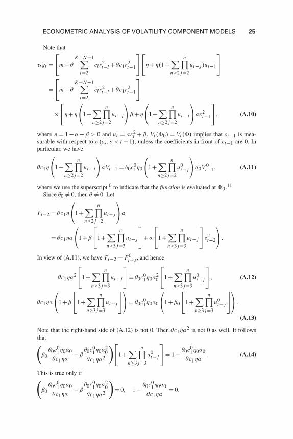
Note that
τt gt =⎡⎣m + θ
K+N−1∑l=2
clr2t−l + θc1r2
t−1
⎤⎦⎡⎣η+η(1+
∑n≥2
n∏j=2
ut− j )ut−1
⎤⎦
=⎡⎣m + θ
K+N−1∑l=2
clr2t−l + θc1r2
t−1
⎤⎦
×⎡⎣η+η
⎛⎝1+
∑n≥2
n∏j=2
ut− j
⎞⎠β +η
⎛⎝1+
∑n≥2
n∏j=2
ut− j
⎞⎠αε2
t−1
⎤⎦ , (A.10)
where η = 1 −α −β > 0 and ut = αε2t +β. Vt ( 0) = Vt ( ) implies that εt−1 is mea-
surable with respect to σ(εs ,s < t − 1), unless the coefficients in front of εt−1 are 0. Inparticular, we have
θc1η
⎛⎝1+
∑n≥2
n∏j=2
ut− j
⎞⎠αVt−1 = θ0c0
1η0
⎛⎝1+
∑n≥2
n∏j=2
u0t− j
⎞⎠α0V 0
t−1, (A.11)
where we use the superscript 0 to indicate that the function is evaluated at 0.11
Since θ0 �= 0, then θ �= 0. Let
Ft−2 = θc1η
⎛⎝1+
∑n≥2
n∏j=2
ut− j
⎞⎠α
= θc1ηα
⎛⎝1+β
⎡⎣1+
∑n≥3
n∏j=3
ut− j
⎤⎦+α
⎡⎣1+
∑n≥3
n∏j=3
ut− j
⎤⎦ε2
t−2
⎞⎠ .
In view of (A.11), we have Ft−2 = F0t−2, and hence
θc1ηα2
⎡⎣1+
∑n≥3
n∏j=3
ut− j
⎤⎦ = θ0c0
1η0α20
⎡⎣1+
∑n≥3
n∏j=3
u0t− j
⎤⎦ , (A.12)
θc1ηα
⎛⎝1+β
⎡⎣1+
∑n≥3
n∏j=3
ut− j
⎤⎦⎞⎠ = θ0c0
1η0α0
⎛⎝1+β0
⎡⎣1+
∑n≥3
n∏j=3
u0t− j
⎤⎦⎞⎠ .
(A.13)
Note that the right-hand side of (A.12) is not 0. Then θc1ηα2 is not 0 as well. It followsthat(
β0θ0c0
1η0α0
θc1ηα−β
θ0c01η0α2
0
θc1ηα2
)⎡⎣1+
∑n≥3
n∏j=3
u0t− j
⎤⎦ = 1− θ0c0
1η0α0
θc1ηα. (A.14)
This is true only if(β0
θ0c01η0α0
θc1ηα−β
θ0c01η0α2
0
θc1ηα2
)= 0, 1− θ0c0
1η0α0
θc1ηα= 0.

26 FANGFANG WANG AND ERIC GHYSELS
Therefore, θc1ηα = θ0c01η0α0, and β/α = β0/α0, and hence (A.12) becomes
α
⎡⎣1+
∑n≥3
n∏j=3
ut− j
⎤⎦ = α0
⎡⎣1+
∑n≥3
n∏j=3
u0t− j
⎤⎦ . (A.15)
Note that the left-hand side of (A.15) is
α2
⎡⎣1+
∑n≥4
n∏j=4
ut− j
⎤⎦ε2
t−3 +α +αβ
⎡⎣1+
∑n≥4
n∏j=4
ut− j
⎤⎦ .
Similarly we have
α2
⎡⎣1+
∑n≥4
n∏j=4
ut− j
⎤⎦ = α2
0
⎡⎣1+
∑n≥4
n∏j=4
u0t− j
⎤⎦ , (A.16)
α +αβ
⎡⎣1+
∑n≥4
n∏j=4
ut− j
⎤⎦ = α0 +α0β0
⎡⎣1+
∑n≥4
n∏j=4
u0t− j
⎤⎦ . (A.17)
It follows that α = α0, and hence β = β0, θc1 = θ0c01, and m − m0 +∑N+K−1
l=2 (θcl −θ0c0
l )r2t−l = 0. In a similar argument and using the fact that
∑N+K−1l=1 cl = N and As-
sumption 4.1, we have m = m0, θ = θ0, and ω = ω0. n
Proof of Lemma 4.4. Note that LT − LT = 1T −(N+K )
∑Tt=N+K+1 log( Vt
Vt) +(
r2t
Vt− r2
t
Vt
)= 1
T −(N+K )
∑Tt=N+K+1 log( gt
gt) + r2
tτt gt
gt −gtgt
. By Cesaro’s Lemma, it suf-
fices to show sup ∈U | log( gtgt
)| and sup ∈U | r2t
τt gt
gt −gtgt
| converge to 0 almost surely.
For t > K + N , because gt = gt + βt−K−N (gK+N − gK+N ) and U is compact, wehave
log
(gt
gt
)≤ gt
gt−1 ≤ 1
1−α −ββ t−K−N gK+N ≤ C∗βt gK+N , (A.18)∣∣∣∣∣ r2
tτt gt
gt − gt
gt
∣∣∣∣∣ ≤ 1
(1−α −β)2mβt−K−N r2
t gK+N ≤ C∗βt r2t gK+N , (A.19)
for some constant C∗ > 0, and β ∈ (0,1). Therefore, we just need to show thatsup ∈U βt gK+N and sup ∈U β t r2
t gK+N converge to 0 almost surely.Note that for any ε > 0,
P( supφ∈U
βt r2t gK+N > ε) ≤ ε−δ∗/2βtδ∗/2(E(r2
t )δ∗)1/2(E sup
φ∈Ugδ∗
K+N )1/2,
where δ∗ is defined in Corollary 3.1. Because E(r2t )δ
∗is finite and E supφ∈U gδ∗
K+N < ∞(due to inequality (A.9)), we have
∞∑t=K+N+1
P( supφ∈U
βt r2t gK+N > ε) < ∞.
ECONOMETRIC ANALYSIS OF VOLATILITY COMPONENT MODELS 27
It follows from the Borel–Cantelli lemma that sup ∈U βt r2t gK+N converges to 0 almost
surely. Similarly, we have sup ∈U βt gK+N converges to 0 almost surely. n
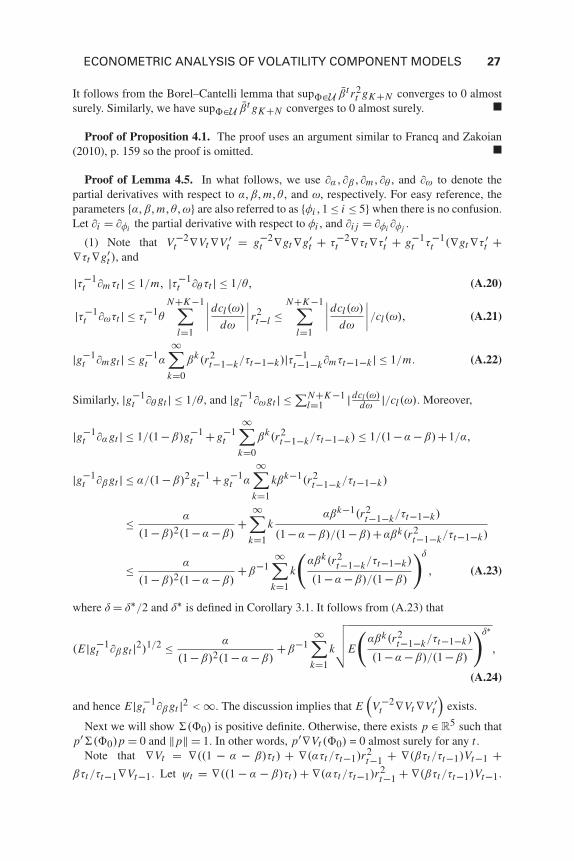
Proof of Proposition 4.1. The proof uses an argument similar to Francq and Zakoian(2010), p. 159 so the proof is omitted. n
Proof of Lemma 4.5. In what follows, we use ∂α,∂β,∂m ,∂θ , and ∂ω to denote thepartial derivatives with respect to α,β,m,θ , and ω, respectively. For easy reference, theparameters {α,β,m,θ,ω} are also referred to as {φi ,1 ≤ i ≤ 5} when there is no confusion.Let ∂i = ∂φi the partial derivative with respect to φi , and ∂i j = ∂φi ∂φj .
(1) Note that V −2t ∇Vt∇V ′
t = g−2t ∇gt∇g′
t + τ−2t ∇τt∇τ ′
t + g−1t τ−1
t (∇gt∇τ ′t +
∇τt∇g′t ), and
|τ−1t ∂mτt | ≤ 1/m, |τ−1
t ∂θ τt | ≤ 1/θ, (A.20)
|τ−1t ∂ωτt | ≤ τ−1
t θ
N+K−1∑l=1
∣∣∣∣dcl (ω)
dω
∣∣∣∣r2t−l ≤
N+K−1∑l=1
∣∣∣∣dcl (ω)
dω
∣∣∣∣/cl (ω), (A.21)
|g−1t ∂m gt | ≤ g−1
t α
∞∑k=0
βk(r2t−1−k/τt−1−k)|τ−1
t−1−k∂mτt−1−k | ≤ 1/m. (A.22)
Similarly, |g−1t ∂θ gt | ≤ 1/θ , and |g−1
t ∂ωgt | ≤ ∑N+K−1l=1 | dcl (ω)
dω |/cl (ω). Moreover,
|g−1t ∂αgt | ≤ 1/(1−β)g−1
t + g−1t
∞∑k=0
βk(r2t−1−k/τt−1−k) ≤ 1/(1−α −β)+1/α,
|g−1t ∂β gt | ≤ α/(1−β)2g−1
t + g−1t α
∞∑k=1
kβk−1(r2t−1−k/τt−1−k)
≤ α
(1−β)2(1−α −β)+
∞∑k=1
kαβk−1(r2
t−1−k/τt−1−k)
(1−α −β)/(1−β)+αβk(r2t−1−k/τt−1−k)
≤ α
(1−β)2(1−α −β)+β−1
∞∑k=1
k
(αβk(r2
t−1−k/τt−1−k)
(1−α −β)/(1−β)
)δ
, (A.23)
where δ = δ∗/2 and δ∗ is defined in Corollary 3.1. It follows from (A.23) that
(E |g−1t ∂β gt |2)1/2 ≤ α
(1−β)2(1−α −β)+β−1
∞∑k=1
k
√√√√E
(αβk(r2
t−1−k/τt−1−k)
(1−α −β)/(1−β)
)δ∗
,
(A.24)
and hence E |g−1t ∂β gt |2 < ∞. The discussion implies that E
(V −2
t ∇Vt∇V ′t
)exists.
Next we will show �( 0) is positive definite. Otherwise, there exists p ∈ R5 such thatp′�( 0)p = 0 and ‖p‖ = 1. In other words, p′∇Vt ( 0) = 0 almost surely for any t.
Note that ∇Vt = ∇((1 − α − β)τt ) + ∇(ατt/τt−1)r2t−1 + ∇(βτt/τt−1)Vt−1 +
βτt/τt−1∇Vt−1. Let ψt = ∇((1 − α − β)τt ) + ∇(ατt/τt−1)r2t−1 + ∇(βτt/τt−1)Vt−1.
28 FANGFANG WANG AND ERIC GHYSELS
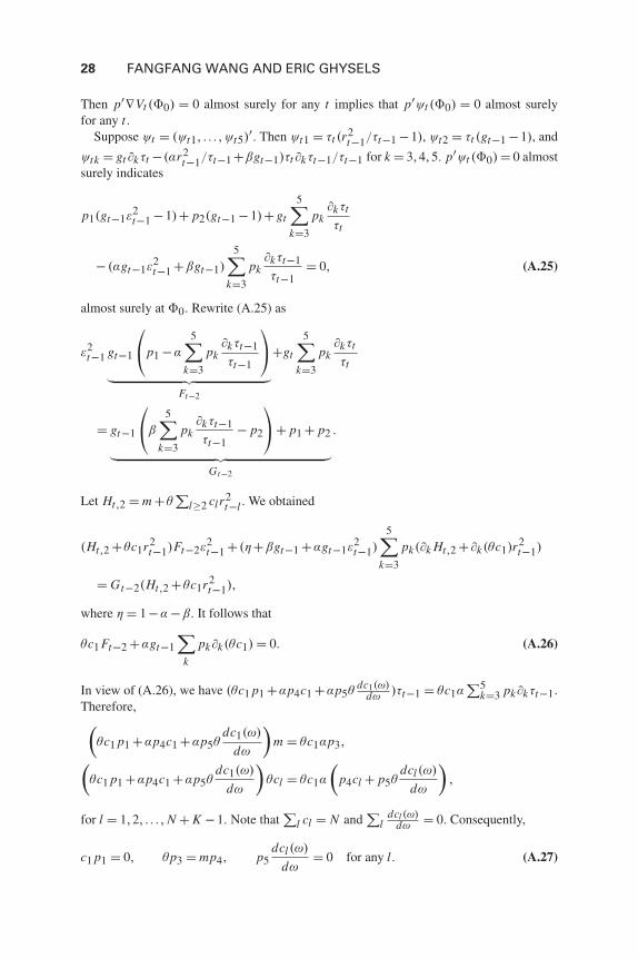
Then p′∇Vt ( 0) = 0 almost surely for any t implies that p′ψt ( 0) = 0 almost surelyfor any t.
Suppose ψt = (ψt1, . . . ,ψt5)′. Then ψt1 = τt (r2t−1/τt−1 −1), ψt2 = τt (gt−1 −1), and
ψtk = gt∂kτt −(αr2t−1/τt−1 +βgt−1)τt∂kτt−1/τt−1 for k = 3,4,5. p′ψt ( 0) = 0 almost
surely indicates
p1(gt−1ε2t−1 −1)+ p2(gt−1 −1)+ gt
5∑k=3
pk∂kτt
τt
− (αgt−1ε2t−1 +βgt−1)
5∑k=3
pk∂kτt−1
τt−1= 0, (A.25)
almost surely at 0. Rewrite (A.25) as
ε2t−1 gt−1
⎛⎝p1 −α
5∑k=3
pk∂kτt−1
τt−1
⎞⎠
︸ ︷︷ ︸Ft−2
+gt
5∑k=3
pk∂kτt
τt
= gt−1
⎛⎝β
5∑k=3
pk∂kτt−1
τt−1− p2
⎞⎠+ p1 + p2
︸ ︷︷ ︸Gt−2
.
Let Ht,2 = m + θ∑
l≥2 clr2t−l . We obtained
(Ht,2 + θc1r2t−1)Ft−2ε2
t−1 + (η+βgt−1 +αgt−1ε2t−1)
5∑k=3
pk(∂k Ht,2 + ∂k(θc1)r2t−1)
= Gt−2(Ht,2 + θc1r2t−1),
where η = 1−α −β. It follows that
θc1 Ft−2 +αgt−1∑
k
pk∂k(θc1) = 0. (A.26)
In view of (A.26), we have (θc1 p1 +αp4c1 +αp5θ dc1(ω)dω )τt−1 = θc1α
∑5k=3 pk∂kτt−1.
Therefore,(θc1 p1 +αp4c1 +αp5θ
dc1(ω)
dω
)m = θc1αp3,(
θc1 p1 +αp4c1 +αp5θdc1(ω)
dω
)θcl = θc1α
(p4cl + p5θ
dcl (ω)
dω
),
for l = 1,2, . . . , N + K −1. Note that∑
l cl = N and∑
ldcl (ω)
dω = 0. Consequently,
c1 p1 = 0, θp3 = mp4, p5dcl (ω)
dω= 0 for any l. (A.27)
ECONOMETRIC ANALYSIS OF VOLATILITY COMPONENT MODELS 29
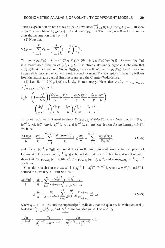
Taking expectation on both sides of (A.25), we have∑5
k=3 pk E(g1∂kτ1/τ1) = 0. In viewof (A.27), we obtained p4 E(gt ) = 0 and hence p4 = 0. Therefore, p ≡ 0 and this contra-dicts the assumption that ‖p‖ = 1.
(2) Note that
∇LT = 1
T
T∑t=1
∇lt = 1
T
T∑t=1
(1− r2
tVt
)∇Vt
Vt.
We have ∂i lt ( 0) = (1 − ε2t )(∂i τt ( 0)/τt ( 0) + ∂i gt ( 0)/gt ( 0)). Because ∂i lt ( 0)
is a measurable function of {ε2s ,s ≤ t}, it is strictly stationary ergodic. Note also that
E(∂i lt ( 0))2 is finite, and E(∂i lt ( 0)|rs ,s < t) = 0. We have {∂i lt ( 0), t ∈ Z} is a mar-tingale difference sequence with finite second moment. The asymptotic normality followsfrom the martingale central limit theorem, and the Cramer–Wold device.
(3) Let Bn = B( 0,1/n) ∩ A. Bn is not empty. Note that ∂i j LT = 1T −(N+K )∑T
t=N+K+1 ∂i j lt , and
∂i j lt =(
1− r2t
τt gt
)(∂i j gt
gt+ ∂i j τt
τt+ ∂i gt
gt
∂j τt
τt+ ∂j gt
gt
∂i τt
τt
)
+(
2r2t
τt gt−1
)(∂i gt
gt+ ∂i τt
τt
)(∂j gt
gt+ ∂j τt
τt
).
To prove (30), we first need to show E sup ∈Bn|∂i ∂j lt ( )| < ∞. Note that |τ−1
t ∂i τt |,|g−1
t ∂αgt |, |g−1t ∂θ gt |, |g−1
t ∂ωgt |, and |g−1t ∂m gt | are bounded on A (see Lemma 4.5(1)).
We have
τt ( 0)
τt= m0
τt+
N+K−1∑l=1
θ0cl (ω0)r2t−l
τt≤ m0
m+
N+K−1∑l=1
θ0cl (ω0)
θcl (ω), (A.28)
and hence |τ−1t τt ( 0)| is bounded as well. An argument similar to the proof of
Lemma 4.5(1) shows that |τ−1t ∂i j τt | is bounded onA as well. Therefore, it is sufficient to
show that E sup ∈Bn|g−1
t gt ( 0)|2, E sup ∈Bn|g−1
t ∂β gt |4, and E sup ∈Bn|g−1
t ∂i j gt |2are finite.
Consider n such that n > n0 ≡ �1 +β−10 (1 −βδ
0)−1/(1−δ)�, where δ = δ∗/4 and δ∗ isdefined in Corollary 3.1. For ∈ Bn ,
gt ( 0)
gt≤ η0
η+
∞∑k=0
α0βk0r2
t−1−k/τ0t−1−k
η+αβkr2t−1−k/τt−1−k
≤ η0
η+ α0
α1−δηδmδ
∞∑k=0
βk0
βk(1−δ)
τt−1−k
τ0t−1−k
r2δt−1−k , (A.29)
where η = 1 −α −β, and the superscript 0 indicates that the quantity is evaluated at 0.Note that η0
η , α0α1−δηδmδ , and τt−1−k
τ 0t−1−k
are bounded on A. For ∈ Bn ,
β0
β(1−δ)≤ β0
β(1−δ)0 −n−(1−δ)
≤ β0
β(1−δ)0 −n−(1−δ)
0
< 1.
30 FANGFANG WANG AND ERIC GHYSELS
Let ρ0 = β0
β(1−δ)0 −n−(1−δ)
0
. Using (A.29), we have sup ∈Bn
g0t
gt≤ K + K
∑∞k=0 ρk
0r2δt−1−k
for some constant K > 0. It follows from Corollary 3.1 that
E sup ∈Bn
|g−1t gt ( 0)|2 < ∞. (A.30)
Take δ appearing in (A.23) as δ∗/4, then in a similar argument we have
E sup ∈Bn
|g−1t ∂β gt |4 < ∞. (A.31)
Moreover, note that ∂αgt = (gt − 1)/α, and ∂ααgt = 0. Therefore, sup ∈Bn|g−1
t ∂αβ gt |,sup ∈Bn
|g−1t ∂αθ gt |, sup ∈Bn
|g−1t ∂αm gt |, sup ∈Bn
|g−1t ∂αωgt | are square integrable.
Note also that∣∣∣∣∂ββ gt
gt
∣∣∣∣ ≤ 2α
(1−β)3η+β−2
∞∑k=2
k(k −1)αβk(r2
t−1−k/τt−1−k)
η+αβk(r2t−1−k/τt−1−k)
≤ 2α
(1−β)3η+β−2
∞∑k=2
k(k −1)
(αβkr2
t−1−k
mη
)δ∗/2
, (A.32)
∣∣∣∣∂βm gt
gt
∣∣∣∣ ≤∞∑
k=1
kαβk−1(r2
t−1−k/τt−1−k)
η+αβk(r2t−1−k/τt−1−k)
∣∣∣∣∂mτt−1−k
τt−1−k
∣∣∣∣≤ 1
mβ
∞∑k=1
k
(αβk(r2
t−1−k/τt−1−k)
η
)δ∗/2
, (A.33)
∣∣∣∣∂mm gt
gt
∣∣∣∣ ≤∞∑
k=0
αβk(r2t−1−k/τt−1−k)
η+αβk(r2t−1−k/τt−1−k)
(2
∣∣∣∣∂mτt−1−k
τt−1−k
∣∣∣∣2 +∣∣∣∣∂mmτt−1−k
τt−1−k
∣∣∣∣)
≤∞∑
k=0
(αβkr2
t−1−k
ητt−1−k
)δ∗/2 (2
∣∣∣∣∂mτt−1−k
τt−1−k
∣∣∣∣2 +∣∣∣∣∂mmτt−1−k
τt−1−k
∣∣∣∣)
. (A.34)
We have E sup ∈Bn|g−1
t ∂ββ gt | < ∞ and E sup ∈Bn|g−1
t ∂βm gt | < ∞ due to (A.20),
Corollary 3.1 and A being compact. Similarly, we have E sup ∈Bn|g−1
t ∂βθ gt |,E sup ∈Bn
|g−1t ∂βωgt |, E sup ∈Bn
|g−1t ∂mθ gt |, E sup ∈Bn
|g−1t ∂mωgt |, and E sup ∈Bn
|g−1t ∂θωgt | are finite.Because ∂i j lt is strictly stationary ergodic—it is a measurable function of {r2
s ,s ≤ t},and
sup ∈Bn
‖H(LT )( )−�( 0)‖ ≤ sup ∈Bn
‖H(LT )( )− E H(l1)( )‖
+ E sup ∈Bn
‖H(l1)( )− H(l1)( 0)‖,
and E sup ∈Bn‖H(lt )( )‖ is O(1) uniformly in t , (30) holds due to the dominated con-
vergence theorem and the uniform SLLN.
ECONOMETRIC ANALYSIS OF VOLATILITY COMPONENT MODELS 31
(4) It suffices to show 1√T
∑Tt=N+K+1 sup ∈A |∂i lt ( )− ∂i lt ( )| converges to 0 in
probability for each i. Note that
|∂i lt − ∂i lt | =∣∣∣∣∣(
1− r2t
Vt
)∂i Vt
Vt−
(1− r2
t
Vt
)∂i Vt
Vt
∣∣∣∣∣≤
∣∣∣∣∣ gt − gt
gt
r2t
Vt
∂i Vt
Vt
∣∣∣∣∣+∣∣∣∣∣(
∂i gt
gt− ∂i gt
gt
)(1− r2
t
Vt
)∣∣∣∣∣ ,∣∣∣∣∂i gt
gt− ∂i gt
gt
∣∣∣∣ ≤ |g−1t ∂i gt |
∣∣∣∣ gt − gt
gt
∣∣∣∣+ g−1t |∂i gt − ∂i gt |,
|∂i gt − ∂i gt | ≤ (t − K − N )β t−K−N−1|gK+N − gK+N |+βt−K−N |∂i gK+N |.
In view of (A.18) and (A.19), we have, for ∈A,
|∂i lt − ∂i lt | ≤ C∗β t r2t gK+N
∣∣∣∣∂i Vt
Vt
∣∣∣∣+C∗βt (|∂i gt |gK+N + t |gK+N − gK+N |+ |∂i gK+N |)
∣∣∣∣∣1− r2t
Vt
∣∣∣∣∣ ,for some constant C∗ > 0 and 0 < β < 1. Therefore, for 0 < δ < 1,
E( sup ∈A
|∂i lt ( )− ∂i lt ( )|)δ ≤ Cδ∗tδβδt E(t,δ), (A.35)
where
E(t,δ) = t−δ E
[sup
∈Ar2t gK+N
∣∣∣∣∂i Vt
Vt
∣∣∣∣+ (|∂i gt |gK+N
+t |gK+N − gK+N |+ |∂i gK+N |)|1− r2t
Vt|]δ
≤ E
[sup
∈Ar2t gK+N
∣∣∣∣∂i Vt
Vt
∣∣∣∣]δ
+ E
[sup
∈A|∂i gt |gK+N
∣∣∣∣∣1− r2t
Vt
∣∣∣∣∣]δ
+ E
[sup
∈A|gK+N − gK+N |
∣∣∣∣∣1− r2t
Vt
∣∣∣∣∣]δ
+ E
[sup
∈A|∂i gK+N |
∣∣∣∣∣1− r2t
Vt
∣∣∣∣∣]δ
.
Note that Er2δ∗t and E(sup ∈A gt )
δ∗ are finite (see Corollary 3.1, (A.9)). In a simi-
lar argument and using the fact that τ−1t ∂i τt is bounded on A, E(sup ∈A ∂i gt )
δ∗ and
E(sup ∈A V −1t ∂i Vt )
δ∗ are finite. Take δ = δ∗/3, then E(t,δ∗/3) is bounded, say by C∗∗.It follows that, ∀ε > 0,
32 FANGFANG WANG AND ERIC GHYSELS
P
⎛⎝ 1√
T
T∑t=N+K+1
sup ∈A
|∂i lt ( )− ∂i lt ( )| > ε
⎞⎠
≤ (√
T ε)−δ∗/3 E
⎡⎣ T∑
t=N+K+1
sup ∈A
|∂i lt ( )− ∂i lt ( )|⎤⎦δ∗/3
≤ (√
T ε)−δ∗/3T∑
t=N+K+1
Cδ∗/3∗ tδ∗/3(βδ∗/3)t C∗∗
−→ 0 as t → ∞.
Therefore, limT →∞√
T sup ∈A ‖∇LT ( )−∇ LT ( )‖ = 0 in probability. n
Proof of Proposition 4.2. We first show that√
T ( T − 0) =⇒ N (0, (Eε4t −
1)�( 0)−1). Note that −∇LT ( 0) = H(LT )( T )( T − 0) where T is between 0 and T . Since T converges to 0 a.s., it follows from Lemma 4.5(3) thatH(LT )( T ) converges to �( 0) a.s. Note that �( 0) is invertible. Therefore,
√T ( T −
0) = −(�( 0))−1(1 + op(1))√
T ∇LT ( 0). The asymptotic normality follows fromLemma 4.5(2) and Slutsky’s theorem.
Next we will show√
T ( T − T ) = op(1). Note that ∇LT ( T ) − ∇LT ( T ) =H(LT )( T )( T − T ) where T is between T and T . On one hand,√
T (∇LT ( T ) − ∇LT ( T )) = √T (∇LT ( T ) − ∇ LT ( T )) converges to 0 in proba-
bility due to Lemma 4.5(4). On the other hand, H(LT )( T ) converges to �( 0) a.s.due to Lemma 4.5(3). Therefore,
√T ( T − T ) = (�( 0))−1(1+op(1))(∇LT ( T )−
∇ LT ( T )) converges to 0 in probability.An application of Slutsky’s theorem yields that
√T ( T − 0) converges to
N (0, (Eε4t −1)�( 0)−1) in distribution. n