Econometrica Supplementary Material

SUPPLEMENT TO “STRUCTURAL CHANGE AND THE KALDORFACTS IN A GROWTH MODEL WITH RELATIVE PRICE EFFECTS

AND NON-GORMAN PREFERENCES”: ONLINE APPENDIX(Econometrica, Vol. 82, No. 6, November 2014, 2167–2196)

BY TIMO BOPPART

APPENDIX B

B.1. Proofs of Lemmas 1–3

B.1.1. Proof of Lemma 1

PROOF: Equation (2) corresponds to the expenditure function

e(PG(t)�PS(t)�Vi(t)

) =[ε

[Vi(t)+ ν

γ

[PG(t)

PS(t)

]γ

+ 1ε

− ν

γ

]]1/ε

PS(t)�(B.1)

First, note that non-negativity of consumption bundles is fulfilled since ∂e(·)∂PG(t)

=ν[ e(·)

PS(t)]1−ε[ PS(t)

PG(t)]1−γ > 0 and ∂e(·)

∂PS(t)= [ e(·)

PS(t)]1−ε[[ e(·)

PS(t)]ε − ν[PG(t)

PS(t)]γ] ≥ 0 is ensured

by (3) (remember that γ ≥ ε). Then, according to the integrability theorem,the utility function represents a locally non-satiated preference relation if andonly if the Slutsky matrix H is symmetric and negative semidefinite and satisfiesH · P = 0, where P is the vector of prices. The Hessian of (B.1) can be writtenas

H = Ξ

⎛⎜⎝

PS(t)

PG(t)−1

−1PG(t)

PS(t)

⎞⎟⎠ �

where Ξ = ν[ e(·)PS(t)

]1−2εPG(t)γ−1PS(t)

−γ[ν(1 − ε)[PG(t)

PS(t)]γ − (1 − γ)[ e(·)

PS(t)]ε]. Sym-

metry and the regularity condition are then straightforward. The eigenvaluesof H are 0 and Ξ[ PS(t)

PG(t)+ PG(t)

PS(t)]. So both eigenvalues are less than or equal

to zero (and the matrix is negative semidefinite) if and only if condition (3)holds. Q.E.D.

B.1.2. Proof of Lemma 2

PROOF: Optimization implies that the marginal rate of technical substitu-tion is equal to the relative factor price, that is, w(t)

R(t)= α

1−α

Kj(t)

Lj(t), j = G�S. With

© 2014 The Econometric Society DOI: 10.3982/ECTA11354

2 TIMO BOPPART

R(t)=A and (9), this gives (12) and (16). Next, R(t) has to equalize the valuedmarginal product across all sectors. This yields

R(t)=A = (1 − α)

[L(t)

KG(t)+KS(t)

]α

Pj(t)exp[gjt]� j =G�S�

where (16) has been used. Solving for Pj(t) gives (14). Finally, with (16), theproduction functions can be rewritten as (15). Q.E.D.

B.1.3. Proof of Lemma 3

PROOF: (i) This proof is an application of Roy’s identity that states xij(t) =

− ∂V (·)/∂Pj(t)∂V (·)/ei(t) for j = G�S. We have ∂V (·)/∂PG(t) = −νPG(t)

γ−1PS(t)−γ ,

∂V (·)/∂PS(t) = −ei(t)εPS(t)

−ε−1 + νPG(t)γPS(t)

−γ−1, and ∂V (·)/ei(t) =ei(t)

ε−1PS(t)−ε.

Part (ii) follows immediately from (17) and (18).(iii) The Allen–Uzawa formula for the elasticity of substitution reads σi(t)=∂2e(·)

∂PS(t) ∂PG(t)

∂e(·)∂PG(t)

∂e(·)∂PS(t)

e(·), where e(·) is the expenditure function defined in (B.1).

Note that ∂e(·)∂PG(t)

and ∂e(·)∂PS(t)

are derived in the proof of Lemma 1 and ∂2e(·)∂PS(t) ∂PG(t)

is given by the off-diagonal element of the Slutsky matrix H. Plugging in theexpressions, simplifying, and substituting e(·) by ei(t), we obtain (19). We haveσi(t)≤ 1 because of (3) and γ ≥ ε. This completes part (iii). Q.E.D.

B.2. The Specified Subclass of PIGL Preferences

The most general (indirect) form of PIGL preferences can be written as (seeMuellbauer (1975))

V (P� ei) = 1ϑ

[ei

a(P)

]ϑ

− b(P)�(B.2)

with ϑ �= 0.1 ei is the expenditure level of household i, P is the price vector,a(P) is a linearly homogeneous function, and b(P) is homogeneous of degreezero. For ϑ = 1 we obtain the Gorman form and for ϑ = −1 the quadratic

1For ϑ= 0, we have the “PIGLOG” case with

V (P� ei) = log[ei]log[a(P)] − b(P)�

where again a(P) is a linearly homogeneous function and b(P) is homogeneous of degree zero(see Muellbauer (1975)).

STRUCTURAL CHANGE AND THE KALDOR FACTS 3

demand system. Finally, with ∂b(P)∂P = 0, we obtain the class of homothetic pref-

erences.In the following, I show that the class of preferences specified in this pa-

per is the most general class of intratemporal preferences defined over twosectors implying a behavior which is jointly consistent with a constant (neg-ative) growth rate of the expenditure share devoted to one sector (see Fig-ure 1) and a constant (positive) growth rate of per-capita expenditures (oneof the Kaldor facts) in an environment where the relative price changes at aconstant rate also (see Figure 2). The PIGL class of preferences is a naturalstarting point because it is the most general class of utility functions whichavoids an aggregation problem. PIGL preferences guarantee that there ex-ists a representative expenditure level in the sense that a household with thisspecific expenditure level exhibits the same expenditure shares as the aggre-gate economy. With PIGL preferences, this representative expenditure levelis just a function of the per-capita expenditure level as well as of a summarystatistic of the expenditure level distribution. Moreover, with additive separa-ble intertemporal utility, as Crossley and Low (2011) showed, it is a necessarycondition that the intratemporal preferences are part of the PIGL class, in or-der for the intertemporal elasticity of substitution to be constant. Since a con-stant intertemporal elasticity of substitution is indispensable to be consistentwith the Kaldor facts, the PIGL class of preferences is the only natural startingpoint.

With (B.2), the marginal utility of consumption expenditures is a(P)−ϑeϑ−1i .

Now suppose that all relative prices change at constant growth rates (as in Ngaiand Pissarides (2007)). Then, in order to fulfill the Kaldor facts, the marginalutility of consumption expenditures (and ei) has to grow at a constant rate,too. With changing relative prices, this is only possible if a(P) = a

∏j P

αjj ,

where the αj ’s sum up to 1 and a is a (positive) constant. Since utility func-tions are invariant with respect to positive monotonic transformations, wecan normalize a = 1 without loss of generality. Then, utility can be rewrittenas

V (P� ei)= 1ϑ

[ei∏

j

Pαjj

]ϑ

− b(P)�

Applying Roy’s identity, we then obtain the following expenditure share de-voted to sector j:

ηij = αj + ∂b(P)

∂Pj

[ei

a(P)

]−ϑ

Pj�

4 TIMO BOPPART

Now suppose the expenditure share of sector j =G changes at a constant rate.This is only possible if we have αG = 0 and b(P) = Pγ

Gb(P), where b(P) is ho-mogeneous of degree −γ and independent of PG.

To sum up, the following conditions must hold in the two-sector case:a(P) = PS and b(P) = ν

γ[PGPS

]γ . Hence, we obtain the functional form of (2),where ϑ= ε. In the paper, the restrictions on γ and ε are chosen such thatthe expenditure elasticity of demand of sector G and the elasticity of substitu-tion between the two sectors are smaller than or equal to unity (which is theempirically relevant case).

B.3. Further Extensions

B.3.1. The Symmetric Counterpart of (2)

Clearly, (2) does exclude the case where both sectors enter the preferencessymmetrically. The symmetric counterpart of (2) can be written as

V (PG�PS� ei)= 1ε

[ei

P GP

1− S

]ε

− ν

γ

[PG

PS

]γ

− 1ε

+ ν

γ�

Then, the regularity conditions are given by

[ei

P GP

1− S

]ε

≥ −ν

[PG

PS

]γ

�

(1 − )

[ei

P GP

1− S

]ε

≥ ν

[PG

PS

]γ

�

[ei

P GP

1− S

]ε

(1 − 2 − γ)− (1 − ε)ν

[PG

PS

]γ

≥ ( − 1)ν

[ei

P GP

1− S

]2ε[PG

PS

]−γ

�

The first two ensure non-negative consumption, whereas the third conditionmakes sure that the Slutsky matrix is negative semidefinite. But—as demon-strated in Appendix B.2 of this supplement—the expenditure share devoted tothe goods sector changes only at a constant rate if = 0. For the symmetriccase, the elasticity of substitution between the two goods is

σi = 1 − ε− (1 − )[γ − (1 − )ε]

1 −ηiG

+ ε+ γ

ηiG

�

where ηiG is the expenditure share of individual i devoted to the goods sector.

STRUCTURAL CHANGE AND THE KALDOR FACTS 5

B.3.2. Adding a Third Sector With a Constant Expenditure Share

By changing the preferences to

V (PG�PH�PS� ei) = 1ε

[ei

PκHP

1−κS

]ε

− ν

γ

[PG

PS

]γ

− 1ε

+ ν

γ�(B.3)

it is possible to allow for a third sector H with an expenditure elasticity ofdemand equal to unity. This implies that the expenditure share of sector H isconstant and equal to κ. We now have all three cases: a luxury S, a necessity G,and a “neutral” sector H. The intratemporal preferences (B.3) are consistentwith balanced growth on the aggregate as long as PH and PS change at constantrates (which may differ).

B.3.3. Hump-Shape Evolution of the Manufacturing Expenditure Share

Suppose we have

V (PM�PF�PS� ei)= 1ε

[ei

PS

]ε

− ν

γ

[P1−ϕF + P1−ϕ

M ]γ/(1−ϕ)

PγS

− 1ε

+ ν

γ�

What is called “goods” in the main text is now represented by a CES aggregatedefined over manufacturing M and food F . Hence, depending on the elasticityof substitution ϕ and relative price evolution between manufacturing and food,there will be an additional structural change within the goods sector. ApplyingRoy’s identity and aggregating gives the following demand system:

Xij = νφ

[E

N

]1−ε

PεS

[P1−ϕF + P1−ϕ

M ]γ/(1−ϕ)

PγS

P−ϕj

P1−ϕF + P1−ϕ

M

� j = M�F�(B.4)

and

XiS = E

NPS

[1 − νφ

[PS

ei

]ε [P1−ϕF + P1−ϕ

M ]γ/(1−ϕ)

PγS

]�(B.5)

The expenditure share devoted to manufacturing can then be expressed as

ηM = ηGηM , where ηG = νφ[ EN]−εPε

S

[P1−ϕF +P

1−ϕM ]γ/(1−ϕ)

PγS

is the expenditure share

of the entire goods sector (i.e., manufacturing plus food) and ηM = P1−ϕM

P1−ϕF +P

1−ϕM

represents manufacturing expenditures relative to total goods expenditures.As in the main text, this framework is consistent with balanced growth as longas the price of the service sector changes at a constant rate (however, the ex-penditure share of the goods sector will no longer decline at a constant rate).Depending on the parameter ϕ and the evolution of the relative price PF

PM,

6 TIMO BOPPART

any dynamic of food’s and manufacturing’s expenditure share can be gener-ated.

In the following, I illustrate that even in the simple case, where the pricesof all sectors change at constant (but potentially different) rates, we can ob-serve a non-monotonic dynamic in the manufacturing expenditure share. Withconstant growth rates of all relative prices, we have

˙ηM(t)

ηM(t)= (1 −ϕ)

[1 − ηM(t)

](gPM − gPF )�(B.6)

Hence, ηM is either monotonically increasing or decreasing, depending onwhether ϕ � 1 and gPM � gPF . Then, the expenditure share devoted to goodsis

ηG(t)

ηG(t)= −ε[gE − n− gPS ] − γ(gPS − gPF )+ γ[gPM − gPF ]ηM(t)�(B.7)

Since ηM(t)

ηM(t)= ηG(t)

ηG(t)+ ˙ηM(t)

ηM(t), the growth rate of the manufacturing sector is a

linear function of ηM(t).In the following, let us assume that ηM is monotonically increasing over time

(since, for instance, ϕ < 1 and gPM > gPF ). Then, ηM(t) is hump-shaped overtime if [

γ − (1 −ϕ)](gPM − gPF ) < 0�

and

−ε[gE − n− gPS ] − γ(gPS − gPF )+ (1 −ϕ)(gPM − gPF ) > 0�

The intuition is that although the expenditure share of the entire goods sectoris monotonically declining due to an income and substitution effect, there isalso a shifting within the good sector away from food towards manufacturing.This shifting within the good sector is strong in the beginning, which leads toan increasing expenditure share of manufacturing. Eventually, however, thedeclining share of goods becomes dominating and ηM declines.

B.4. Steady State With Neoclassical Production Functions WithIdentical Labor Intensities

Suppose the production functions are

YG(t)= AG(t)F[KG(t)�exp(gt)LG(t)

]�(B.8)

YS(t)= exp(gSt)F[KS(t)�exp(gt)LS(t)

]�(B.9)

STRUCTURAL CHANGE AND THE KALDOR FACTS 7

and

YI(t)= F[KI(t)�exp(gt)LI(t)

]�(B.10)

instead of (7) and (8). g is the exogenous rate of Harrod-neutral technicalprogress and F[·] is an identical neoclassical production function across sectors(with constant returns to scale and positive but diminishing marginal products).AG(t) and exp(gSt) are consumption sector specific Hicks-neutral productiv-ity terms which are time-varying. Because the neoclassical production func-tion F[·] is identical, changes in the Hicks-neutral productivity terms will one-to-one determine changes in relative prices. If the Hicks-neutral productivityterms are not time-varying, we have the same specifications as in Kongsamut,Rebelo, and Xie (2001) and Foellmi and Zweimueller (2008), which abstractfrom relative price effects. If F[·] is a Cobb–Douglas, there is no differencebetween Hicks-neutral and Harrod-neutral technical change and the specifiedtechnologies coincide with the ones in Ngai and Pissarides (2007).

For the growth rates of relative prices, we have

gPG(t)− gPS(t)= gS − AG(t)

AG(t)and gPI (t)− gPS(t)= gS�

Since the production functions are identical apart from the Hicks-neutral pro-ductivity terms, capital intensities must equalize across sectors, that is,

kj(t)≡ Kj(t)

exp(gt)Lj(t)= k(t)� j =G�S� I�

where k(t) ≡ K(t)

exp(gt)L(t) is capital per efficiency units of labor. As in the maintext, we chose the price of the investment good as a numéraire. Since F[·] hasconstant returns to scale, we can write the firms’ first order conditions as

r(t)= f ′(k(t)) − δ and w(t)= exp(gt)[f(k(t)

) − k(t)f ′(k(t))]�where f (k(t)) ≡ F[k(t)�1]. Asset market clearing implies

∫ 10 ai(t)di = K(t)

N(t)=

k(t)exp(gt)L(0). Summing up both sides of (26) over all households and plug-ging in the expressions for the interest and wage rate and using the asset marketclearing condition, we get

k(t)= f(k(t)

) − k(t)[δ+ n+ g] − e(t)�(B.11)

where e(t) ≡ E(t)

exp(gt)L(t) is detrended per-capita consumption. In terms of de-trended variables, the Euler equation and the transversality conditions are

˙e(t)e(t)

= f ′(k(t))− δ− ρ+ εgS

1 − ε− g�(B.12)

8 TIMO BOPPART

and

limt→∞

k(t)exp[−

∫ t

0f ′(k(ς)) − δ− n− g dς

]= 0�(B.13)

For a given k(0), equations (B.11)–(B.13) define the aggregate equilibrium dy-namics. If gS = 0 (and the relative price between service and investment gooddoes not change), these equations are identical to the ones in a one-sector neo-classical growth model with exogenous Harrod-neutral technical progress. IfgS �= 0, an additional constant shows up in the Euler equation but the systemof differential equations remains qualitatively identical. (For this, we see that itis crucial that the Harrod-neutral technical progress in the service sector occursat a constant rate. In contrast, Harrod-neutral progress in the good sector andconsequently the growth rate of the relative price between good and servicescan change over time.)

There exists a globally stable steady state where the detrended k(t) ande(t) are constant. The steady state values are implicitly given by f ′(k∗) =δ+ρ−εgS +(1−ε)g and e∗ = f (k∗)−k∗[δ+n+ g]. In the steady state, the ag-gregate capital stock, expenditure, and output grow at the constant rate g + n.To ensure finite utility and the transversality condition, we need ρ−n > εg andf ′(k∗) > δ− n− g.

For g = A−δ−ρ+εgS1−(1−α)ε

, gS = gS −αg, and AG(t)

AG(t)= gG −αg, ∀t, the growth rates of

E(t), K(t), ηG(t), PG(t), PS(t), and w(t) in the steady state are quantitativelyidentical to the ones in Proposition 2 in the main text.

B.5. Modeling the Input–Output Structure

Suppose that the final investment good, consumption good, and service areproduced according to the technology

Yj(t)=Aj(t)Φj

(Xva

G�j�XvaS�j�X

vaI�j

)� j = G�S� I�

where XvaG�j�X

vaS�j , and Xva

I�j are value-added of the consumption good, service,and investment good sector used to produce final output of sector j. Φj(·) isa neoclassical production function and Aj(t) is a sector specific Hicks-neutralproductivity term. Given the production function, firm’s optimization will tellyou how much U.S. $ value-added of industry G�S, and I is generated if oneU.S. $ is spent on final uses of sector j. For CES production functions Φj(·),this link between value-added and final output is illustrated in equations (6)and (7) in Herrendorf, Rogerson, and Valentinyi (2013). Suppose the value-added production function of sector j can be written as

Yvaj = F

[Kj(t)�exp[gt]Lj(t)

]� j =G�S� I�

STRUCTURAL CHANGE AND THE KALDOR FACTS 9

where Kj(t) and Lj(t) are capital and labor used in value-added industryj = G�S� I. Xj

G(t), XjS(t), and X

jI(t) are consumption goods, services, and in-

vestment goods used as intermediate inputs by sector j. Then, it is fully speci-fied what spending a U.S. $ on final use j implies in terms of factor employmenton the sectoral value-added level.

If Aj(t) = exp[gjt] and Φj(·) and F[·] are Cobb–Douglas, the derived pro-duction functions in terms of final output are Cobb–Douglas also and themodel is consistent with balanced growth on the aggregate. This is identicalto the result in Ngai and Pissarides (2007), who showed in Sections IV and Vhow intermediate inputs or several capital goods can be introduced in theirframework. (See also Ngai and Samaniego (2009) for an empirical applicationwith the Cobb–Douglas intermediate input structure.)

Alternatively, as long as AS(t) = exp(gSt) and AI(t) = 1, the reduced formof the final output production function is

YG(t)=AG(t)F[KG(t)�exp[gt]LG(t)

]�(B.14)

YS(t)= exp(gSt)F[KS(t)�exp(gt)LS(t)

]�(B.15)

and

YI(t)= F[KI(t)�exp(gt)LI(t)

]�(B.16)

where Kj(t) and Lj(t) are factors used in all value-added industries to producefinal output j. This coincides with the reduced form analyzed in Appendix B.4of this supplement. So the model would still be consistent with balanced growthon the aggregate.

B.6. Equilibrium Dynamics With Factor Intensity Differences

Suppose that, instead of (7), the technologies are

Yj(t)= exp[gjt]ααjj (1 − αj)

1−αjLj(t)

αjKj(t)1−αj � j =G�S�

with αj ∈ (0�1), j = G�S, and αG �= αS . We assume that the relative factor en-dowments are the same for all households, that is, ai(0)

li= K(0)

L(0) , ∀i. Under thisassumption, changes in the expenditure shares—which will now affect the rel-ative factor reward R(t)

w(t)—do not affect the inequality measurement φ.2 Finally,

we assume that condition (3) holds with strict inequality.3

2Without this assumption, the joint li and ai(0) distribution would have to be specified andmultiple equilibria could potentially arise.

3This assumption shortens the subsequent proofs, since a separate discussion of the case inwhich—by coincidence—ηG(0) = 1 can be avoided.

10 TIMO BOPPART

With factor intensity differences, Lemma 2 will not hold anymore. To-gether with zero profits and market clearing, firms’ cost minimization yieldsw(t)LG(t) = αGηG(t)E(t) and w(t)LS(t) = αS[1 − ηG(t)]E(t). Combiningthese expressions with the labor market clearing condition gives

w(t)= E(t)

L(t)

[αS +ηG(t)[αG − αS]

]�(B.17)

The AK technology of the investment goods sector is unchanged. Conse-quently, we still have r =R− δ=A− δ. Equilibrium prices are given by

Pj(t)= exp[−gjt]w(t)αjA1−αj � j = G�S�(B.18)

Combining (23) with (B.17), (B.18), and the definition of L(t), we obtain

ηG(t)= ν

[E(t)

L(t)

]αGγ−(γ−ε)αS−ε

L(0)−ε[αS +ηG(t)(αG−αS)

]αGγ−(γ−ε)αS �(B.19)

where ν ≡ νφAε+αS(γ−ε)−αGγ exp[((γ − ε)gS − γgG)t]. Differentiating (B.19)with respect to time gives

ηG(t)

ηG(t)= γ

[E(t)

E(t)− n

]+ (γ − ε)gS − γgG(B.20)

+ [γ + ε] ηG(t)[αG − αS]αS +ηG(t)[αG − αS] �

where γ ≡ αGγ − (γ − ε)αS − ε. With (B.17) and (B.18), the Euler equation(25) can be written as

[1−ε(1−αS)

][ E(t)E(t)

−n

]=A−δ−ρ+εgS − εαSηG(t)[αG − αS]

αS +ηG(t)[αG − αS] �(B.21)

Finally, the law of motion of the capital stock is given by K(t)

K(t)=A−δ+ w(t)L(t)

K(t)−

E(t)

K(t). With (B.17), this can be written as

K(t)

K(t)=A− δ− E(t)

K(t)

[1 − αS −ηG(t)(αG − αS)

]�(B.22)

Equations (B.20), (B.21), (B.22) and the transversality condition define theevolution of ηG(t), E(t), and K(t). K(0) is exogenously given. The non-predetermined E(0) implicitly pins down ηG(0) according to (B.19).4

4For any given E(t), a unique ηG(t) ∈ (0�1) fulfills (B.19). To see this, note that at ηG(t) = 0,the left-hand side (LHS) of (B.19) is zero, whereas the right-hand side (RHS) is ∈ (0�1) (the

STRUCTURAL CHANGE AND THE KALDOR FACTS 11

A constant growth path (CGP) is defined according to Acemoglu and Guer-rieri (2008) as an equilibrium growth path along which expenditures grow at aconstant rate. We have the following proposition:

PROPOSITION 1: Suppose we have

(γ − ε)gS − γgG + [αGγ − (γ − ε)αS − ε

]A− δ− ρ+ εgS

1 − (1 − αS)ε< 0�(B.23)

and let us denote asymptotic values by a superscript A (i.e., zA = limt→∞ z(t),for z = ηG�gE�gK�gw�gηG

). Then, there exists a globally saddle-path stable CGPwith

ηAG = 0�

gAE − n = gA

K − n = gAw = A− δ− ρ+ εgS

1 − (1 − αS)ε�

gAηG

= (γ − ε)gS − γgG + [αGγ − (γ − ε)αS − ε

][gAE − n

]< 0�

PROOF: With the expressions for gAE and gA

ηG, (B.20) and (B.21) can be

rewritten as

ηG(t)

ηG(t)=

[E(t)

E(t)− gA

E

]γ + (γ + ε)

ηG(t)[αG − αS]αS +ηG(t)[αG − αS] + gA

ηG�

and

E(t)

E(t)− gA

E = − εαSηG(t)[αG − αS][1 − ε(1 − αS)][αS +ηG(t)[αG − αS]] �(B.24)

Solving these two equations for ηG(t) gives

ηG(t)=gAηGηG(t)

[ηG(t)+ αS

αG − αS

]αS

αG − αS

+ηG(t)

[1 − (γ + ε)+ αSε

γ

q

] �

upper bound is ensured by the strict inequality of condition (3)). On the contrary, with ηG(t) =1 we have LHS = 1 > RHS. Hence, since both are continuous functions, there is at least oneintersection between 0 and 1. Finally, since the LHS is linear and the RHS is either concave orconvex on the entire domain, we have at most two intersections. Hence, LHS and RHS crossexactly once between 0 and 1.

12 TIMO BOPPART

where q ≡ 1 − ε(1 − αS). Hence, ηG(t) is zero if and only if ηG(t) = 0 (notethat ηG(t) ∈ [0�1]). The equilibrium with ηG(t)= ηG(t)= 0 is stable since

∂ηG(t)

∂ηG(t)

∣∣∣∣ηG(t)=0

= gAηG

< 0�

Hence, no matter where we start, ηG(t) will always converge to ηAG = 0 and

consequently E(t)

E(t)will converge to gA

E (see (B.24)). Hence, asymptotically we

have K(t)

K(t)= A − δ − E(t)

K(t)[1 − αS] and E(t) grows at a constant rate. This is

exactly the same structure as in the equilibrium of the main text. Then, by thesame argument as in the proof of Proposition 2, the transversality condition isviolated unless K(t)

K(t)= E(t)

E(t). Q.E.D.

The CGP is very similar to the one in Acemoglu and Guerrieri (2008). But,the important difference to Acemoglu and Guerrieri (2008) is that this modelfeatures an income effect (as long as ε > 0). In contrast to the asymptotic equi-librium in the main text (see Proposition 3), the structural change is now alsogoverned by the sectoral differences in the output elasticities of labor. Theintuition is the same as in Acemoglu and Guerrieri (2008): We have capitaldeepening, whereby the relative factor price of labor, w(t)

R(t), increases over time.

This increases the relative price of the sector, which is more labor intensive.Finally, according to the substitution effect, this relative price drift affects thestructural change. Condition (B.23) ensures gA

ηG< 0 and guarantees global sta-

bility.

B.7. Relating φ to an Atkinson Index

The Atkinson index (Atkinson (1970)) is defined as

IA

(ζ�

{ei(t)

}1

i=0

) = 1 − N(t)

E(t)

[∫ 1

0ei(t)

1−ζ di

]1/(1−ζ)

�

with the parameter ζ ≥ 0 being the relative inequality aversion. Then, we canwrite

φ(t)= [1 − IA

(ε�

{ei(t)

}1

i=0

)]1−ε�

that is, φ is a negative, monotonic transformation of the Atkinson inequalityindex with ζ = ε. Hence, φ is ordinally equivalent to the inverse of an Atkin-son index. This justifies our interpretation of φ as an inverse measurement ofexpenditure inequality fulfilling the principle of transfers, scale invariance, anddecomposability (see Cowell (2000)).

STRUCTURAL CHANGE AND THE KALDOR FACTS 13

B.8. Data Sources, Description, and Sample Selection

This section documents the data sources and the construction of the vari-ables as well as the selection of the samples. The paper uses the following datasources:

• Bureau of Economic Analysis (BEA): The BEA divides total personal con-sumption expenditure of the United States into “goods” and “services” (seeBEA’s NIPA Table 1.1.5). At the most detailed level of consumption expen-diture categories, this classification can be seen in the underlying detail Ta-ble 2.4.5U. The classification follows the recommendations of the System ofNational Accounts (SNA), which ensures international comparability. More-over, the BEA provides price indices for the different expenditure categories(see NIPA Table 1.1.4) and the corresponding real quantities (see NIPA Ta-ble 1.1.3). Finally, the population data are taken from NIPA Table 7.1. Thepaper uses the yearly data of the years 1946–2012.

In NIPA Tables 1.1.3–1.1.5, the BEA differentiates between durable andnon-durable goods. Figures B.8–B.10 in this supplement show the trend in theexpenditure share, relative price, and relative real quantity if durable goodsare excluded.

• Consumer Expenditure Survey (CEX): The paper uses the CEX survey dataafter the introduction of the “NEW ID” in 1986. The data of the years 1986–2010 are obtained from ICPSR. The data of the year 2011 are obtained di-rectly from the Bureau of Labor Statistics (BLS). The expenditure of a specifichousehold over a 3 month period is considered as an observation. The BEA’sclassification of total personal consumption expenditures into goods and ser-vices is redone with the CEX data. This replication is subject to smaller consis-tency issues due to differences in the level of aggregation. Moreover, one hasto keep in mind that the BEA data include purchases by nonprofit institutionsserving households and by U.S. government civilian and military personnel sta-tioned abroad, whereas the CEX data only cover household expenditure. Also,some fringe benefit payments made by an employer are accounted in the BEAdata, but are not reported in the CEX data.

The following CEX categories are considered as services: food away fromhome; shelter; utilities, fuels and public services; other vehicle expenses; pub-lic transportation; health care; personal care; education; cash contributions;personal insurance; and pensions. For homeowners, the imputed renting valueis taken as shelter expenditures. The remaining categories are considered asgoods. I drop all observations with missing income/transfer reports (177,000observations), non-positive food expenditures (additional 1,006 observations),or with an expenditure share of goods /∈ [0�1] (additional 99 observations).This leaves me with 477,730 observations (i.e., 3 month expenditure spells and177,419 households).

In each year, I group the observations into five income quintiles according tothe total household labor earnings after taxes plus transfers per OECD mod-

14 TIMO BOPPART

ified equivalence scale. For each quintile q = 1� � � � �5, the (average) expendi-ture share of goods is calculated as

ηqG(t)= 1

|Nq(t)|∑

i∈Nq(t)

ηiG(t)�(B.25)

and the average expenditure per-equivalence scale is calculated as

eq(t)= 1|Nq(t)|

∑i∈Nq(t)

ei(t)�(B.26)

where Nq(t) is the set of households that belong to quintile q in year t. Figure 4plots ηq

G(t) for q = 1� � � � �5 and t = 1986� � � � �2011. Figure 7 shows the scatterplot between logηq

G(t) and logeq(t) for all quintiles and years (after allowingfor a distinct intercept for each year).

The regressions in columns (1) and (2) in Table I are on the disaggregatelevel. The additional controls in column (2) are: “Children share” and “El-derly share,” which measure the share of household members with age < 18and ≥ 65, respectively. “Residence indicators,” which consist of four regionalindicators (northeast; midwest; south; west), a rural/urban dummy as well asindicators of different population sizes of the city of residence (more than 4M;1.2–4M; 0.33–1.19M; 125–329.9k; less than 125k). “Family size indicators” con-sists of 11 groups (family size of one, two, . . . , ten and above ten). And finally“Ref. person controls,” which consist of the age, the sex, seven skill level in-dicators (never attended school; elementary school; high school, less than h.s.graduate; h.s. graduate; college, less than college graduate; college graduate(associate’s D. and bachelor’s D.); graduate school (master’s D. and Profes-sional/Doctorate’s D.)) and four race indicators (white; black; native american;asian) of the reference person.

In columns (4) and (5) of Table I, durable goods are excluded. The follow-ing categories are considered as durable goods: old and new vehicles; housefurnishing, and equipment.

This supplement provides the regressions corresponding to columns (1) and(2) in Table I with CEX diary data of the year 2010. In the diary data, thelogarithmized labor and capital earnings after taxes and deductions plus trans-fers per equivalent scale is used as an instrument for the expenditure level.The following categories are considered as service: shelter (mortgage pay-ments, rents and buying of land and houses); food and drinks away fromhome; fuels and electricity, public services; clothing repair services; vehicleleasing; vehicle repair and maintenance services; house maintenance services;healthcare services; entertainment services; sports equipment rental; personalcare; school tuition. The remaining categories are considered as “goods.” Ob-

STRUCTURAL CHANGE AND THE KALDOR FACTS 15

servations are monthly expenditures of a particular household. The regres-sions include month fixed effects. The sample selection and the additionalcontrol variables in column (2) of Table B.II are identical to the ones in Ta-ble I.

• Panel Study of Income Dynamics (PSID): The PSID wave of 2009 in-cludes relatively detailed expenditure data. The following expenditure cate-gories are considered as “goods”: Food at Home (F12, F18, F22), Car Pur-chase Cash-down Payments (F64), Car Loan Payments (F67), Car Lease Pay-ments (F71, F72), Additional Car/Lease Payments (F79), Gasoline (F80B),Household Furnishings (F88), and Clothing (F89). The following expendi-ture categories are considered as “services”: Property Tax Expenses (A21),Owner Insurance (A22), Mortgage Payments (A25), Rent (A31), Home Re-pairs (F87), Utilities (A41–A45B), Health Insurance (H63), Hospital/NursingHome Expenses (H64), Doctor/Outpatient Surgery/Dental Expenses (H70),Prescriptions/Other Medical Services (H76), Donations (M2A–M12B), ChildCare (F6D), Food Delivered to Home (F20, F24), Food Eaten Out (F21, F25),Car Insurance (F77), Car Repair (F80A), Parking (F80C), Bus/Train Fares(F81A), Cab Fares (F81B), Other Transportation Expenses (F81C), SchoolExpenses (F83), Other School Expenses (F86), Trips/Vacations (F90), OtherRecreation (F91), Support of Others (G106), and Voluntary Pension Contri-butions of Head and Wife (P15, P85). Since expenditures of different cate-gories are reported for different time intervals, all expenditures are annual-ized. The expenditure share of goods is “good expenditure” relative to “goodexpenditure” plus “service expenditure.” These PSID data are used in column(3) of Table I. The logarithmized expenditure level per equivalent scale is in-strumented by the logarithmized “Total Labor Income” plus “Total TransferIncome” plus “Social Security Income” per OECD equivalent scale. “Chil-dren share” and “Elderly share” are measured as in the CEX data. “Resi-dence indicators” consist of five regional indicators (northeast; northcentral;south; west; alaska&hawaii) as well as six indicators of different populationsizes of the city of residence (Central counties of at least 1M population;Fringe counties of at least 1M population; Counties in metropolitan areas;Urban population of 20k or more; Urban population of less than 20k; Com-pletely rural areas). “Family size indicators” consist of the same 11 groups asin the CEX data. “Family head controls” consist of the age, the sex, seven skilllevel indicators (constructed as in the CEX data), and seven race indicators(white; black; hispanic; indian; asian; pacific-islander; other-race) of the family“head.”

• Eurostat: As the BEA data, the expenditure data are based on the Classifi-cation of Individual Consumption by Purpose (COICOP) recommended by theSystem of National Accounts (SNA). From Eurostat I, use the 3 digit COICOPexpenditure and price data (see tables “nama_co3_c” and “nama_co3_p”). Thefollowing categories are considered as “goods”: Food and non-alcoholic bev-erages; Alcoholic beverages, tobacco, and narcotics; Clothing and footwear;

16 TIMO BOPPART

Electricity, gas, and other fuels; Furnishings, household equipment, and rou-tine maintenance of the house; Medical products, appliances, and equipment;Purchase of vehicles; Telephone and telefax equipment; Audio-visual, pho-tographic, and information processing equipment; Other major durables forrecreation and culture; Other recreational items and equipment, gardens, andpets; Newspapers, books, and stationery; Personal care products; and Per-sonal effects n.e.c. The following categories are considered as “service”: Ac-tual rentals for housing; Imputed rentals for housing; Maintenance and re-pair of the dwelling; Water supply and miscellaneous services relating to thedwelling; Out-patient services; Hospital services; Operation of personal trans-port equipment; Transport services; Postal services; Telephone and telefax ser-vices; Recreational and cultural services; Package holidays; Education; Restau-rants and hotels; Social protection; Insurance; Financial services n.e.c.; andOther services n.e.c. The category “Prostitution” is excluded since there aretoo many missing values. At this disaggregate level, Eurostat provides datafor the following 23 countries: Austria, Belgium, Czech Republic, Denmark,Finland, France, Germany, Greece, Hungary, Iceland, Ireland, Italy, Luxem-bourg, Netherlands, Norway, Poland, Portugal, Slovakia, Slovenia, Spain, Swe-den, and United Kingdom. These 23 countries and the BEA data of the UnitedStates are included in Figure B.12. Eurostat provides price indices for thedifferent expenditure subcategories (although for a shorter time period forsome countries). The price index of “goods” and “services” is calculated asa Fisher chained price index. The real quantities are calculated as the nom-inal expenditure of goods/services divided by the corresponding price index.The ratio of the price indices is plotted in Figure B.13. The relative realquantity of services is illustrated in Figure B.14. Due to the lack of reliableprice data on the disaggrate level, Portugal is not included in these two fig-ures.

• Living Costs and Food Survey (LCF): In Figures B.3 and B.4, I use U.K.survey data provided in the “Family Spending” files by Office for NationalStatistics (ONS). The expenditure categories of recent years are not com-parable with the years before 2001/2002. So I use data covering the years2001–2011. In each year, the households are grouped into the five quin-tiles according to gross family income. For each income quintile, I calcu-late the average weekly expenditure per capita by aggregating “all expen-diture groups 1–12” and dividing by “number of persons per household.”Expenditure on “goods” is defined as “all expenditure groups 1–12” minus“housing (4),” “health (6),” “transport (7),” “communication (8),” “recre-ation & culture (9),” “education (10),” and “restaurant & hotel (11).” Theexpenditure share on goods of quintile i is calculated as the sum of ex-penditures on “goods” of all households belonging to quintile i divided bythe sum of “all expenditure groups 1–12” of households belonging to quin-tile i.

STRUCTURAL CHANGE AND THE KALDOR FACTS 17

B.9. Additional Figures and Tables

FIGURE B.1.—Cross-sectional variation excluding shelter. The figure plots the expenditureshare devoted to goods for each income quintile of the U.S. on a logarithmic scale when shelterexpenditures are excluded. As in Figure 4, the quintiles refer to total household labor earningsafter tax plus transfers per OECD modified equivalence scale. The sample consists of expendi-ture data of 477,730 quarters (and 177,419 households). Source: Consumer Expenditure Surveyinterview data obtained from the BLS for the year 2011 and from the ICPSR for all other years.

18 TIMO BOPPART

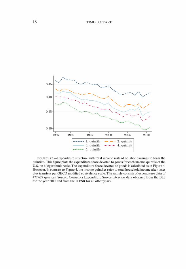
FIGURE B.2.—Expenditure structure with total income instead of labor earnings to form thequintiles. This figure plots the expenditure share devoted to goods for each income quintile of theU.S. on a logarithmic scale. The expenditure share devoted to goods is calculated as in Figure 4.However, in contrast to Figure 4, the income quintiles refer to total household income after taxesplus transfers per OECD modified equivalence scale. The sample consists of expenditure data of477,627 quarters. Source: Consumer Expenditure Survey interview data obtained from the BLSfor the year 2011 and from the ICPSR for all other years.

STRUCTURAL CHANGE AND THE KALDOR FACTS 19

FIGURE B.3.—Cross-sectional variation in U.K. data. The figure plots the expenditure sharedevoted to goods for each income quintile of the U.K. on a logarithmic scale. The followingexpenditure categories are considered as services: housing, health, transport, communication,recreation & culture, education, restaurant & hotel. All other categories are considered as goods.The income quintiles refer to gross household income. Source: ONS, Living Costs and FoodSurvey (LCF).

20 TIMO BOPPART

FIGURE B.4.—Scatter plot of cross-sectional variation in U.K. data. The figure depicts thepartial correlation between the logarithmized average weekly expenditure level per householdmember and the logarithmized average expenditure share of goods of a given income quintile,where we allowed in each year for a separate (distinct) intercept. The slope of the fitted lineis −0�1892. This slope is the same as if we regressed the logarithmized expenditure share onthe logarithmized expenditure level per household member and time dummies. The R2 of thisunderlying regression is 0�8731 and the standard error of the slope coefficient is 0�0114. Source:ONS, Living Costs and Food Survey (LCF).

STRUCTURAL CHANGE AND THE KALDOR FACTS 21

FIGURE B.5.—Per-capita expenditures in terms of services. The figure plots per-capita per-sonal consumption expenditures in terms of services in the U.S. on a logarithmic scale. The priceof services is normalized to 1 in the year 2005. The dashed line represents the predicted values ob-tained by regressing the logarithmized expenditures on time and a constant. The estimated slopecoefficient and its standard error are 0�0156 and 0�00028. respectively. The regression attains anR2 of 0�9791. Source: BEA, NIPA Tables 1.1.4 and 1.1.5 as well as Table 7.1 for the populationdata.

22 TIMO BOPPART

FIGURE B.6.—Estimates of ε over time. The figure plots the estimates for ε and its 95 percentconfidence band obtained by running the specification of column (2) of Table I for each yearseparately. The regressions include quarter fixed effects.

STRUCTURAL CHANGE AND THE KALDOR FACTS 23

FIGURE B.7.—Share of goods versus aggregate per-capita expenditures. The figure depicts thescatter plot between per-capita personal consumption expenditures in terms of services and theexpenditure share devoted to goods in the United States. Both axes are measured on a logarith-mic scale. The price of services is normalized to 1 in the year 2005. The red dashed line representsthe predicted values obtained by regressing the logarithmized expenditure share on the logarith-mized per-capita expenditures and a constant. The estimated slope coefficient and its standarderror are −0�6301 and 0�0166, respectively. The absolute value of this slope can be interpreted asthe required ε if we want to explain the entire structural change solely by an income effect. (See(23) and note that the slope in this figure is in line with (40) and γ = 0.) The simple regressionattains an R2 of 0�9570. Source: BEA, NIPA Tables 1.1.4 and 1.1.5 as well as Table 7.1 for thepopulation data. The black dashed line is the predicted share of goods with ε= 0�2222, which weestimated in the cross-section (see Figure 7). We see that the model can—even with γ = 0—fitthe aggregate data pretty well. However, this requires an ε which is, compared to cross-sectionaldata, inconsistently high. I would like to thank Richard Rogerson for suggesting to illustrate thiscomparison.

24 TIMO BOPPART

FIGURE B.8.—Expenditure share of non-durable goods. The figure plots the share of personalconsumption expenditures devoted to non-durable goods in the United States on a logarithmicscale. The dashed line represents the predicted values obtained by regressing the logarithmizedexpenditure share on time and a constant. The estimated slope coefficient and its standard errorare −0�0135 and 0�00025, respectively. The regression attains an R2 of 0�9787. Source: BEA,NIPA Table 1.1.5.

STRUCTURAL CHANGE AND THE KALDOR FACTS 25

FIGURE B.9.—Relative price between non-durable goods and services. The figure plots therelative consumer price between non-durable goods and services on a logarithmic scale. Thedashed line represents the predicted values obtained by regressing the logarithmized relativeprice on a constant and time. The estimated slope coefficient and its standard error are −0�0110and 0�00030, respectively. The regression attains an R2 of 0�9532. Source: BEA, NIPA Table 1.1.4.

26 TIMO BOPPART

FIGURE B.10.—Real quantity of services relative to non-durable goods. The figure plots thereal quantity of services relative to non-durable goods, XG(t), on a logarithmic scale. The relativequantity is normalized to 1 in the year 1946. Source: BEA, NIPA Table 1.1.3.

STRUCTURAL CHANGE AND THE KALDOR FACTS 27

FIGURE B.11.—Cross-sectional variation excluding durables. The figure plots the expenditureshare devoted to goods for each income quintile of the United States on a logarithmic scale whendurable goods are excluded. As in Figure 4, the quintiles refer to total household labor earningsafter tax plus transfers per OECD modified equivalence scale. The sample consists of expendituredata of 425,402 quarters. Source: Consumer Expenditure Survey interview data obtained from theBLS for the year 2011 and from the ICPSR for all other years.

28 TIMO BOPPART

FIGURE B.12.—Expenditure share of goods: OECD countries. The figure plots the expendi-ture share of goods on a logarithmic scale in 23 European OECD countries and the United States.If we regress in the OECD sample (excluding the U.S.) the logarithm of the share of goods on acountry fixed effect and the year, the slope coefficient is −0�0087 with a standard error of 0�0001.The R2 of the regression is 0�9295. Source: Eurostat and BEA.

STRUCTURAL CHANGE AND THE KALDOR FACTS 29

FIGURE B.13.—Relative price of goods: OECD countries. The figure plots the relative price ofgoods on a logarithmic scale in 22 European OECD countries and the United States. The relativeprice is normalized to 1 in the year 2005. If we regress in the OECD sample (excluding the U.S.)the logarithm of the relative price on a country fixed effect and the year, the slope coefficient is−0�0138 with a standard error of 0�0003. The R2 of the regression is 0�8472. Source: Eurostat andBEA.

30 TIMO BOPPART

FIGURE B.14.—Relative real quantity of services: OECD countries. The figure plots the realquantity of services relative to goods on a logarithmic scale of 22 European OECD countries andthe United States. The relative quantity is normalized to 1 in the year 2000. Source: Eurostat andBEA.

STRUCTURAL CHANGE AND THE KALDOR FACTS 31

FIGURE B.15.—Predicting the late rise of the service economy. The blue dashed line repre-sents the expenditure share devoted to services, 1 − ηG(t), in the BEA data back to 1929. Thered line is the model’s implied expenditure share using ε = 0�182 and γ = 0�410 (as suggestedby the cross-sectional estimation) as well as the observed relative prices PG(t)

PS(t)and per-capita ex-

penditure in terms of services E(t)N(t)PS(t)

. The green dashed line represents the share of servicesin value-added as in Buera and Kaboski (2012b). The level difference comes from the fact thatthe BEA categorizes final consumption expenditures into goods and services, whereas for thevalue-added data, industries are categorized as services or manufacturing. Source: BEA, NIPATables 1.1.4, 1.1.5, and 7.1 and Buera and Kaboski (2012b) for the value-added data.

32 TIMO BOPPART

FIGURE B.16.—Stone–Geary’s prediction. The blue dashed line represents the expen-diture share devoted to services, 1 − ηG(t), in the BEA data back to 1929. The redline is—as in Figure B.15—the cross-sectional back in time prediction using this pa-per’s functional form. The green dashed line represents the back in time predictionif we use the function form implied by a “generalized Stone–Geary” utility functionU(XG(t)�XS(t)) = [ω1/σ

G (XG(t) − XG)(σ−1)/σ + (1 − ωG)

1/σXS(t)(σ−1)/σ ]σ/(σ−1). This func-

tional form implies for the expenditure share of goods of the representative agent:ηG(t) = ωGPG(t)1−σ

ωGPG(t)1−σ+(1−ωG)PS(t)1−σ + (1−ωG)PS(t)1−σ

ωGPG(t)1−σ+(1−ωG)PS(t)1−σ [ XGPG(t)N(t)

E(t)]. Estimating this functional

form by nonlinear least squares using cross-sectional data of the different income quintiles

1986–2011 gives: ωG = 0�285, σ = 0�719, and ˆXG = 649�19. ˆXG can be interpreted as quarterlysubsistence spending per-equivalent scale in 2005 good prices. The subsistence spending are (onaverage) 16.37 percent in 1986. (All the estimates are comparable to the ones in Herrendorf,Rogerson, and Valentinyi (2013). Adding a (potentially negative) subsistence level in servicesleaves the fit unchanged.) Calibrating the per-capita subsistence spending, XGPG(t)N(t)

E(t), to 16.37

percent in 1986 and ω and σ to the values of 0.285 and 0.719, the green dashed line showsthe predicted expenditure share spent on services using aggregate BEA data. The generalizedStone–Geary specification implies that an asymptotic expenditure elasticity of demand is unityfor all sectors. Consequently, relatively large subsistence levels are needed in order to get rea-sonable income effects in later years. But these required subsistence levels imply an even largerincome effect in earlier years and the model generates rather the opposite of a “late rise of theservice sector.”

STRUCTURAL CHANGE AND THE KALDOR FACTS 33

TABLE B.I

CROSS-SECTIONAL ESTIMATION OF ε WITH TOTAL INCOME AS THE INSTRUMENTa

(1) (2)

− logei(t) 0�205∗∗∗ 0�195∗∗∗

(0.002) (0.003)Children share 0�128∗∗∗

(0.004)Elderly share −0�042∗∗∗

(0.003)Residence indicators No YesFamily size indicators No YesRef. person controls No Yes

Observations 477,627 425,315R2 0.013 0.047Method IV IV

aDependent variable: logηiG(t). Standard errors in parentheses. ∗∗∗ significant at 1 percent, ∗∗ significant at 5

percent, ∗ significant at 10 percent. All regressions include quarter fixed effects (104 groups). The logarithmizedexpenditure level per equivalent scale is instrumented by the logarithmized total income after taxes plus transfersper equivalent scale. “Children share” and “Elderly share” measure the share of household members with age < 18and ≥ 65, respectively. “Residence indicators” consists of regional indicators (four groups), a rural/urban dummy,as well as indicators of different population densities of the city of residence (five groups). “Family size indicators”consists of 11 groups. “Ref. person controls” consists of the age, the sex, skill-level indicators (seven groups) and raceindicators (four groups) of the reference person.

34 TIMO BOPPART

TABLE B.II

CROSS-SECTIONAL ESTIMATION OF ε USING DIARY DATA OF THE YEAR 2010a

(1) (2)

− logei(t) 0�244∗∗∗ 0�300∗∗∗

(0.025) (0.039)Children share 0.025

(0.058)Elderly share −0�023

(0.041)Residence indicators No YesFamily size indicators No YesRef. person controls No Yes

Observations 9,050 9,017R2 0.206 0.225Method IV IV

aDependent variable: logηiG(t). Standard errors in parentheses. ∗∗∗ significant at 1 percent, ∗∗ significant at 5

percent, ∗ significant at 10 percent. All regressions include month fixed effects (12 groups). The logarithmized ex-penditure level per equivalent scale is instrumented by the logarithmized labor and capital earnings after taxes anddeductions plus transfers per equivalent scale. The following broad expenditure categories are considered as services:shelter (mortgage payments, rents and buying of land and houses); food and drinks away from home; fuels and elec-tricity, public services; clothing repair services; vehicle leasing; vehicle repair and maintenance services; house main-tenance services; healthcare services; entertainment services; sports equipment rental; personal care; school tuition.“Children share” and “Elderly share” measure the share of household members with age < 18 and ≥ 65, respectively.“Residence indicators” consists of regional indicators (four groups), a rural/urban dummy, as well as indicators ofdifferent population densities of the city of residence (five groups). “Family size indicators” consist of 11 groups. “Ref.person controls” consists of the age, the sex, skill-level indicators (seven groups), and race indicators (four groups) ofthe reference person. Source: Diary data of the Consumer Expenditure Survey from the Bureau of Labor Statistics.

STRUCTURAL CHANGE AND THE KALDOR FACTS 35

ADDITIONAL REFERENCES

COWELL, F. A. (2000): “Measurement of Inequality,” in Handbook of Income Distribution, ed. byA. B. Atkinson and F. Bourguignon. Amsterdam: North-Holland. [12]

CROSSLEY, T., AND H. LOW (2011): “Is the Elasticity of Intertemporal Substitution Constant?”Journal of the European Economic Association, 9 (1), 87–105. [3]

NGAI, L. R., AND R. M. SAMANIEGO (2009): “Mapping Prices Into Productivity in MultisectorGrowth Models,” Journal of Economic Growth, 14 (3), 183–204. [9]

Institute for International Economic Studies, Stockholm University, 106 91Stockholm, Sweden and Dept. of Economics, University of Zurich; timo.boppart@iies.su.se.

Manuscript received January, 2013; final revision received June, 2014.