econometrica, vol. 75, no. 4 (july, 2007),...
TRANSCRIPT

Econometrica, Vol. 75, No. 4 (July, 2007), 993–1038
PRICES AND PORTFOLIO CHOICES IN FINANCIAL MARKETS:THEORY, ECONOMETRICS, EXPERIMENTS
BY PETER BOSSAERTS, CHARLES PLOTT, AND WILLIAM R. ZAME1
Many tests of asset-pricing models address only the pricing predictions, but thesepricing predictions rest on portfolio choice predictions that seem obviously wrong. Thispaper suggests a new approach to asset pricing and portfolio choices based on unob-served heterogeneity. This approach yields the standard pricing conclusions of classicalmodels but is consistent with very different portfolio choices. Novel econometric testslink the price and portfolio predictions and take into account the general equilibriumeffects of sample-size bias. This paper works through the approach in detail for thecase of the classical capital asset pricing model (CAPM), producing a model calledCAPM + ε. When these econometric tests are applied to data generated by large-scalelaboratory asset markets that reveal both prices and portfolio choices, CAPM+ε is notrejected.
KEYWORDS: Experimental finance, experimental asset markets, risk aversion.
1. INTRODUCTION
MANY ASSET-PRICING MODELS predict both asset prices and portfolio choices.For instance, the classical capital asset pricing model (CAPM) predicts port-folio separation (that all agents should hold the market portfolio), while Mer-ton’s (1973) continuous-time model and Connor’s (1984) equilibrium versionof APT both predict k-fund separation.2 Forty years of econometric tests ofsuch models present varying levels of support for the pricing predictions ofthese models, but even casual empiricism suggests that the portfolio choicepredictions are badly wrong. Because the pricing predictions of these modelsare built on the portfolio choice predictions (through the assumption that port-folio choices are optimal given prices), the pricing predictions and the portfo-lio choice predictions seem inextricably linked, and it therefore seems hard totake the pricing predictions seriously while ignoring the portfolio choice pre-dictions.
1We thank seminar audiences at the Atlanta Finance Forum, Bachelier Finance Society In-ternational Congress, CMU, CEPR, CIDE, Erasmus University, Harvard University, Insead,IDEI, London Business School, NBER, RFS Conference on Behavioral and Experimental Fi-nance, Rice University, SWET, UC Berkeley, UCLA, UC Riverside, University of Chicago GSB,University of Copenhagen, USC, and University of Texas (Austin) for comments, and the R. G.Jenkins Family Fund, the National Science Foundation, the Caltech Laboratory for ExperimentalEconomics and Political Science, the John Simon Guggenheim Foundation, the Social and Infor-mation Sciences Laboratory at Caltech, the UCLA Academic Senate Commitee on Research,and the Swiss Finance Institute for financial support. Opinions, findings, conclusions, and recom-mendations expressed in this material are those of the authors and do not necessarily reflect theviews of any funding agency.
2Even the Fama–French three factor model (Davis, Fama, and French (2002)) assumes thatinvestors only hold combinations of three basic portfolios.
993

994 P. BOSSAERTS, C. PLOTT, AND W. R. ZAME
This paper suggests a new approach to asset pricing and portfolio choicethat allows both to be taken seriously. Our approach maintains the essentialparsimony of existing models, but adds unobserved heterogeneity. Applied toany of the models above, our approach would yield models that have identi-cal pricing implications but are consistent with very different portfolio choices.(In particular, this approach suggests a rationale for testing pricing predictionswithout testing portfolio choice predictions.) Although our approach could beapplied to a wide range of models, we choose here to apply it only to the classi-cal CAPM, yielding a model we call CAPM+ε. The CAPM is a convenient andpractical starting point because it is the simplest model that is consistent withobserved prices in our experimental data; given the level of risk and rewardin our experiments, other classical models would yield similar predictions (seeJudd and Guu (2001) for instance). The CAPM + ε differs from the standardCAPM in assuming that demand functions of individual traders can be decom-posed as sums of mean–variance components and idiosyncratic components,and that the idiosyncratic components are drawn from a distribution that hasmean zero. These idiosyncratic components can be interpreted as reflectingunobserved heterogeneity of preferences; this is an approach similar to thatused in much applied work. (The name CAPM +ε is suggested by viewing truedemand functions as perturbations of mean–variance demand functions.) Weconstruct econometric tests of CAPM + ε, and apply those tests to data gen-erated by experimental financial markets in which both prices and portfoliochoices can be observed. The CAPM + ε does well on these data: it is rejected(by either of our tests) at the 1% level in only one sample in eight and at the5% level in only two samples in eight.
We arrange our presentation in the following way. We begin (Section 2) bydescribing CAPM + ε and providing a simple theoretical analysis to show thatCAPM + ε yields the standard pricing conclusions of classical models but isconsistent with very different portfolio choices.3
With this simple theoretical analysis in hand, we next (Section 3) extend fa-miliar analyses of models of individual choice to derive econometric tests ofour model. We make use of the model assumption that individual demandfunctions can be decomposed into mean–variance components, and idiosyn-cratic components, and that the idiosyncratic components are random (whichprovides a source of variation) and from a distribution that has mean zero.
3In a continuum economy, the idiosyncratic components of demand would exactly average outacross the population and prices would be exactly as predicted by CAPM, but portfolio choicesmight be much different. In a large but finite economy, an appropriate form of the law of largenumbers implies that the idiosyncratic components of demand will (with high probability) almostaverage out across the population. Using this, we show that (with high probability) prices willbe near to those predicted by CAPM, but again, portfolio choices may be much different. Theargument is not difficult, but it is not trivial, because the competitive equilibrium correspondenceis not continuous; hence a small perturbation might cause equilibria to disappear. The result weneed depends on the fact that the CAPM equilibrium of the continuum economy is regular.

CHOICES IN FINANCIAL MARKETS 995
Our tests are based on the generalized method of moments (GMM), adaptedto large cross sections, rather than long time series. Our tests are novel in anumber of ways:• Our tests link prices and choices.• In the usual models of choice with unobserved heterogeneity, the null hy-
pothesis is that the idiosyncratic components of demand have mean zeroand are orthogonal to prices. In our setting, the idiosyncratic componentsof demand functions have mean zero and are orthogonal to prices. How-ever, because demands influence equilibrium prices, the realizations of theidiosyncratic components of demand functions need not be orthogonal toprices. This induces a significant small-sample bias. Our tests accommodatethis bias, by allowing for a Pitman drift under the null hypothesis. As a re-sult, the asymptotic distribution of our GMM test statistic is noncentral χ2.(Absent the small-sample bias, the asymptotic distribution would be centralχ2.)
• To compute the weighting matrix for our GMM statistic, we need esti-mates of individual risk tolerances (inverses of risk aversion coefficients).Inspired by techniques introduced by McFadden (1989) and Pakes and Pol-lard (1989), we obtain individual risk tolerances using (unbiased) ordinaryleast squares (OLS) estimation. Because the error averages out across sub-jects, this strategy enables us to ignore the (fairly large) error in estimatingindividual risk tolerances.The next part of our presentation (Section 4) describes our experimental
asset markets. Experimental asset markets are ideal for our purpose becausethey make it possible to observe (or control) many parameters that are difficultor impossible to observe in the historical data, including the market portfolio,the true distribution of returns, the information held by investors, and portfo-lio choices. In each of our experimental markets, 30–60 subjects trade risklessand risky securities (whose dividends depend on the state of nature) and cash.Each experiment is divided into 6–9 periods. At the beginning of each period,subjects are endowed with a portfolio of securities and cash. During the period,subjects trade through a continuous, web-based open-book system (a form ofdouble auction that keeps track of inframarginal bids and offers). After a pre-specified time, trading halts, the state of nature is drawn, and subjects are paidaccording to their terminal holdings. The entire situation is repeated in eachperiod but states are drawn independently at the end of each period. Subjectsknow the dividend structure (the payoff of each security in each state of na-ture) and the probability that each state will occur, and of course they knowtheir own holdings and their own attitudes toward wealth and risk. They alsohave access to the history of orders and trades. Subjects do not know the num-ber of participants in any given experiment, the holdings of other participants,or the market portfolio (the aggregate supply of risky securities).
In Section 5, we present our analysis of the experimental data. We fol-low standard strategy, which is familiar from empirical studies of historical
996 P. BOSSAERTS, C. PLOTT, AND W. R. ZAME
data, and use end-of-period prices and portfolio holdings, ignoring intraperiodprices.4 Our experiments actually represent an environment that is closer toa static asset-pricing model than are typical studies of historical data, becauseour securities have only one-period lives. We can use liquidating dividends assecurity payoffs, while empirical tests of historical data usually take the rel-atively arbitrary end of the month as the end of the period, and use prices(including dividends collected during the month) as security payoffs.
Because the subject population is constant during an experiment, differentperiods within a single experiment do not represent independent draws. How-ever, because subject populations of different experiments are disjoint, identi-cal periods of different experiments do represent independent draws. We usethis fact to construct multiple independent samples by using data across ex-periments. From these samples we construct empirical distributions of our teststatistic and use standard (Kolmogorov–Smirnov and Cramer–von Mises) teststo measure the goodness-of-fit of these empirical distributions with a noncen-tral χ2 distribution function. The summary results are that the Kolmogorov–Smirnov and Cramer–von Mises goodness-of-fit tests reject CAPM + ε at the1% level in only one of eight samples and reject at the 5% level in only twoof eight samples. These results are especially striking in comparison to othertests of asset-pricing models, which frequently reject at the 0.5% level. BecauseMonte Carlo methods are neither practical nor appropriate in this context, weprovide an alternative power analysis based on perturbations of the existingdata (rather than on artificial data, which Monte Carlo methods would utilize).This analysis suggests that our tests have significant power: relatively small per-turbations of prices lead to many more rejections.
Following all of this, Section 6 concludes. Technical details are relegated tovarious appendixes.
2. CAPM + ε
In this section, we offer a model that makes pricing predictions close to thatof the classical CAPM but is consistent with very different portfolio choices.Our starting point is suggested by the idea—familiar from applied work—that parametric specifications of preferences represent only a convenient ap-proximation of the observed/expressed/true demand structure in the market-place. We implement this idea by viewing observed demands as perturbationsof “ideal” demands (hence the name CAPM + ε). In principle, these perturba-tions might represent some combination of subject errors (in computing andimplementing optimal choices), market frictions, and unobserved heterogene-ity. Because an adequate treatment of errors or market frictions would neces-sitate a fully stochastic model, which we are not prepared to offer, and because
4This is not to say that intraperiod prices are of no interest; see Asparouhova, Bossaerts, andPlott (2003) and Bossaerts and Plott (2004) for detailed discussions.

CHOICES IN FINANCIAL MARKETS 997
we have some evidence that errors and market frictions are not of most impor-tance in our setting (but see Bossaerts, Plott, and Zame (2002)), we focus hereon unobserved heterogeneity.
Because the approach we follow is quite intuitive (there is only one smallsubtle issue), the following informal description is sufficient for our needs. Tofix ideas, we first formalize equilibrium in asset markets, and recall the stan-dard development of the classical CAPM in a particular context appropriate toour experiments. (Appendix A fills in some missing details.) We then presentthe formal model, which adds perturbations to individual demands. (Appen-dix B presents a careful and rigorous justification.)
2.1. Equilibrium in Asset Markets
In our experiments, two risky assets and a riskless asset (notes) are tradedagainst cash. Because cash and notes have the same payoffs, we treat themas redundant assets, and use a model with two risky assets and one risklessasset. Thus, in our model, investors trade assets A, B, and N , which are claimsto state-dependent consumption. In our experiments, there are three states ofnature: X , Y , and Z. We write divA for the state-dependent dividends of assetA, divA(s) for dividends in state s, and so forth. If θ = (θA�θB�θN) ∈ R
3 is aportfolio of assets, we write
divθ = θA(divA)+ θB(divB)+ θN(divN)
for the state-dependent dividends on the portfolio θ.There are I investors. Investor i is characterized by an endowment portfolio
ωi = (ωiA�ω
iB;ωi
N) ∈ R2+ × R of risky and riskless assets, and a strictly concave,
strictly monotone utility function Ui : R3 → R defined over state-dependentterminal consumptions. (To be consistent with our experimental design, we al-low consumption to be negative.) Endowments and holdings of risky assets areconstrained to be nonnegative, but endowments and holdings of the risklessasset can be negative. In particular, risky assets cannot be sold short, but theriskless asset can be. Investors care about portfolio choices only through theconsumption they yield, so given asset prices q, investor i chooses a portfolioθi to maximize Ui(divθi) subject to the budget constraint q · θi ≤ q ·ωi.
An equilibrium consists of asset prices q ∈ R3++ and portfolio choices θi ∈
R2+ × R for each investor such that:
• Choices are budget feasible: for each i,
q · θi ≤ q ·ωi�
• Choices are budget optimal: for each i
ϕ ∈ R2+ × R� Ui(divϕ) >Ui(divθi) ⇒ q ·ϕ> q ·ωi�

998 P. BOSSAERTS, C. PLOTT, AND W. R. ZAME
• Asset markets clear:
I∑i=1
θi =I∑
i=1
ωi�
2.2. CAPM
The classical CAPM assumes investor i’s utility function for state-dependentwealth x has the (linear) mean–variance form
Ui(x) =E(x)− bi
2var(x)�(1)
where expectations and variances are computed with respect to the true prob-abilities, and bi is absolute risk aversion.5 As usual, it is assumed throughoutthat risk aversion is sufficiently small that the utility functions Ui are strictlymonotone in the range of feasible consumptions (or at least observed con-sumptions).
The assumption of mean–variance utility, in conjunction with the other as-sumptions made above, are very nearly those of the capital asset pricing model;the only difference is that we allow for short sales only of riskless assets, whilethe classical CAPM allows for short sales of both riskless and risky assets. Aswe show in Appendix A, however, if the covariance of the risky assets A andB is negative—as it is in our experimental asset markets and as we henceforthassume—short sales of risky assets are irrelevant and the usual consequencesof CAPM obtain. To describe these consequences briefly (see Appendix Afor further detail), write M = ∑
ωi for the market portfolio of all assets, writem= ∑
(ωiA�ω
iB) for the market portfolio of risky assets, and write M =M/I and
m = m/I for the respective per capita portfolios. Write µ = (E(A)�E(B)) forthe vector of expected dividends of risky assets and
∆ =(
cov[A�A] cov[A�B]cov[B�A] cov[B�B]
)for the covariance matrix of risky assets. It is convenient to normalize so thatthe price of the riskless asset is 1, so that (pA�pB�1) = (p�1) is the vector ofall asset prices. Abusing notation, write asset demands as functions of (p�1)or as functions of p, as is convenient. Write Zi(p) for investor i’s demand forall assets at prices p and write zi(p) for investor i’s demand for risky assets atprices p.
5A frequently used alternative assumption is that agents maximize expected utility with respectto a quadratic felicity function. At the scale of our experiments, the differences would be almostunobservable; we use the mean–variance specification only for econometric convenience. SeeJudd and Guu (2001).

CHOICES IN FINANCIAL MARKETS 999
CAPM equilibrium prices p for risky assets and equilibrium demands aregiven by the formulas
p= µ−(
1I
I∑i=1
1bi
)−1
∆m�(2)
zi(p)= 1bi∆−1(µ− p)�(3)
(The quantity ( 1I
∑ 1bi)−1 is frequently called the market risk aversion and
( 1I
∑ 1bi) is frequently called the market risk tolerance.) Because the demand
and pricing formulas involve individual risk aversions, which are not directlyobservable, they are not testable. However, the following immediate conse-quences of these formulas are testable.• Mean–Variance Efficiency: The market portfolio m of risky assets is mean–
variance efficient; that is, the expected excess return E(divm) − q · m onthe portfolio m is highest among all portfolios that have variance no greaterthan var(divm).6�7
• Portfolio Separation: All investors hold a portfolio of risky assets that is anonnegative multiple of the market portfolio m of risky assets.All of the predictions derived above depend on the assumption that investors
are strictly risk averse: bi > 0. It is not obvious that subjects will display strictrisk aversion in a laboratory setting. However, this is ultimately an empiricalquestion, not a theoretical one. As we shall see later, our own data suggeststrongly that individuals are risk averse. This is not a new finding; see Holt andLaury (2002) for instance.
2.3. Perturbations: CAPM + ε
The classical CAPM assumes that investor i’s utility function Ui has themean–variance form (1). However, we can always write an arbitrary utilityfunction Ui as a perturbation of a mean–variance utility function U i and,hence, can view investor i’s observed/expressed/true demand function zi as aperturbation of a mean–variance demand function zi:
zi(p)= zi(p)+ εi(p)�
Hence, we can model the observed economy as a perturbation of an “ideal”economy that differs only in that investors have mean–variance utilities. (Note
6Because M and m differ only by riskless assets, the entire market portfolio M is also mean–variance efficient.
7There are other pricing implications of CAPM (for instance, the linear beta pricing rule) but,as shown by Roll (1977), these are all consequences of mean–variance efficiency.
1000 P. BOSSAERTS, C. PLOTT, AND W. R. ZAME
that in the ideal economy, investor preferences differ only by the coefficient ofabsolute risk aversion, but that in the observed economy, investor preferencesmay be arbitrary.) Write D and D for the mean market excess demand func-tions for risky assets in the observed economy and in the ideal economy. Bydefinition,
D(p) = 1I
∑(zi(p)−ωi)
= 1I
∑(zi(p)+ εi(p)−ωi)
= 1I
(∑zi(p)−
∑ωi
)+ 1
I
∑εi(p)
= D(p)+ 1I
∑εi(p)�
All this is simply formal manipulation. The economic content of our modelis in the following two assumptions:
(i) The characteristics (asset endowments ωi and demand functions zi) ofinvestors in the observed economy are drawn independently from some distri-bution of characteristics.
(ii) The perturbations εi are drawn independently from a distribution withmean zero.The first of these assumptions is innocuous; the second has real bite. To see theimplications of these assumptions, note first that, by definition, an equilibriumprice is a zero of mean market excess demand. Thus, if the mean perturbation1I
∑εi is identically zero, then equilibrium prices in the observed economy and
in the ideal economy will exactly coincide. More generally, if the mean pertur-bation 1
I
∑εi is uniformly small, then equilibrium prices in the observed econ-
omy and in the ideal economy will nearly coincide. (Because the equilibriumcorrespondence is not lower hemicontinuous in the parameters of an econ-omy, this is not entirely obvious. The proof relies on the fact that the CAPMequilibrium is regular; see Appendix B.) Because the perturbations are drawnindependently from a distribution with mean zero, a suitable version of thestrong law of large numbers in an appropriate function space will guaranteethat if the number I of investors is sufficiently large, then, with high probabil-ity, the mean perturbation 1
I
∑εi will be uniformly small. In view of CAPM,
the market portfolio of the ideal economy will be mean–variance efficient atthe equilibrium price p for the ideal economy. Because the market portfoliofor the observed economy is the same as the market portfolio for the idealeconomy, if the number I of investors is large then, with high probability, themarket portfolio for the observed economy will be approximately mean–varianceefficient at the equilibrium price for the observed economy. Of course, individualportfolio choices in the observed economy need bear no obvious relationship

CHOICES IN FINANCIAL MARKETS 1001
to individual portfolio choices in the ideal economy; in particular, because theperturbations εi need not be small, approximate portfolio separation need nothold in the observed economy.
Perhaps the most important feature of this model is that it provides a mech-anism that leads to mean–variance efficiency of the market portfolio eventhough no single investor chooses a mean–variance optimal portfolio. (In theclassical CAPM of course, the market portfolio is mean–variance optimal be-cause every investor chooses a mean–variance optimal portfolio.)
Because the pricing conclusions in our model are driven by the strong law oflarge numbers, our model suggests that the likelihood that CAPM pricing willbe observed is increasing in the number of market participants. Experimentalevidence for this suggestion can be found in Bossaerts and Plott (2001).
3. STRUCTURAL ECONOMETRIC TESTS
In this section, we construct a structural econometric test of CAPM +ε. Ourapproach has a number of novel features, some of which distinguish it fromfamiliar econometric approaches to historical price data:• The usual approaches rely entirely on market prices; our approach links
market prices and individual holdings.• In the usual approaches, the source of randomness is the error in estima-
tion of the distribution of returns. In our approach, the source of random-ness is the deviations of observed choices from ideal mean–variance-optimalchoices.
• In the usual approach, generalized method of moments is used to constructan estimator that has good properties for long time series. In our approach,GMM is adapted to construct an estimator that has good properties for largecross sections.8
• The usual approach is to test a theory on each sample separately and thenaggregate the results. Our approach is to construct samples across exper-iments, use our theory to infer the class of distribution to which our teststatistic should belong, and use measures of goodness-of-fit to determinewhether the empirical distribution of our test statistic on these samples isgenerated by a member of this class.Our approach requires estimates of risk aversion for each individual. To ob-
tain such estimates, we use observed choices in other periods of a given exper-iment. Because the number of periods is small, such estimates are necessarily
8We use this approach for two reasons. The first is that we do not have long time series—ourexperiments are only 6–9 periods long—but we do have a large cross section—each experimentinvolves 30–60 subjects. The second reason is that the periods of our experiment do not representindependent draws, because they are populated by the same subjects.

1002 P. BOSSAERTS, C. PLOTT, AND W. R. ZAME
inaccurate; however, our estimation procedure is such that errors across sub-jects tend to cancel out.9
Our approach is inspired by econometric analysis of choice in panel data, butthere is an important difference. In traditional analysis of models of individualchoice, the error term is assumed to be independent of the explanatory vari-ables. In CAPM + ε, the error terms are perturbations of demand functionsand the explanatory variables include prices, but the definition of equilibriumentails that individual demands sum to supply, so that the perturbations cannotbe independent of prices. This is a consequence of the fact that we have a finitepopulation. In an infinite population, independent draws of perturbations froma distribution that has mean zero would yield an aggregate perturbation thatis identically zero, hence independent of prices. We therefore introduce a Pit-man drift to capture the finite-sample bias in the large-sample analysis of ourtest statistic, which leads to an asymptotic distribution of our GMM statisticthat is noncentral χ2. Because we do not have detailed information about theperturbation terms, we do not know the value of the noncentrality parameter.To get around this problem, we will exploit the fact that our various experi-ments provide several independent replications with the same market parame-ters but nonoverlapping populations and thus represent independent draws.Each of these replications generates a sample. We can then test whether theempirical distribution of the GMM test statistics across samples is generatedby some member of the family of noncentral χ2 distributions; this will be ourtest of the CAPM + ε.
3.1. The Null Hypothesis
We focus for the moment on an economy Et that represents a single periodt of a single experiment, in which there are I subjects/investors. Investor i ischaracterized by an endowment ωi and a demand function for risky assets zi
t .10
As in Section 2, we write µ for the vector of mean payoffs of the risky assets,write ∆ for the covariance matrix of payoffs of risky assets, and write mI forthe per capita market portfolio of risky securities. (We write zi
t with a time sub-script and mI with a population superscript as reminders that we focus on aparticular period of a particular experiment. However, we do not subscript orsuperscript the parameters ωi, µ, and ∆ because they do not depend on theparticular period or experiment.) Because endowments ωi are fixed through-out the experiment, we suppress them in what follows.
For each i, let bit be the coefficient of risk aversion that most closely matches
investor i’s end-of-period asset choices in other periods of the same experiment,
9This approach is reminiscent of the method used to obtain consistent standard errors in themethod of simulated moments with only a limited number of simulations per observation; seeMcFadden (1989) and Pakes and Pollard (1989).
10As in Section 4 and Appendix B, we view the characteristics of the subjects as independentdraws from a population with a given distribution.

CHOICES IN FINANCIAL MARKETS 1003
and let zit be the demand function for risky assets for an ideal investor who has
the same endowment as trader i and a mean–variance utility function as in(1) with coefficient of risk aversion bi
t . The difference between the observeddemand function zi
t and the ideal demand function zit is the perturbation or
error:
εit = zit − zi
t �(4)
Let Et be the ideal economy populated by these mean–variance traders. Write
BIt =
(1I
I∑i=1
1bit
)−1
for the market risk aversion for the ideal economy Et . (We use the superscriptI to emphasize that we have an economy with I investors.)
The assumptions of CAPM hold in the ideal economy Et , so write pIt for the
CAPM equilibrium price (again emphasizing dependence on I and t). At equi-librium, per capita demand for risky assets must equal the per capita marketportfolio of risky assets, so rewriting (3) in the present notation yields
zit(p
It )= 1
bit
∆−1(µ− pIt )�(5)
As we show in Appendix A, it follows that pIt = µ−BI
t ∆mI and (assuming that
‖pIt − pI
t ‖ is not too large)
zit(p
It )= 1
bit
∆−1(µ−pIt )�(6)
Assuming that end-of-period prices pIt are actually equilibrium prices for the
economy Et , per capita demand must equal the per capita market portfolio:
1I
∑zit(p
It )= mI�(7)
Summing (5) and (6) over all investors i, combining with (7), and doing a littlealgebra yields the relationship
pIt = pI
t +BIt ∆
1I
I∑i=1
εit(pIt )�(8)
Note that prices pIt appear on both sides of this equation, so it is not a formula
for equilibrium prices.

1004 P. BOSSAERTS, C. PLOTT, AND W. R. ZAME
A familiar intuition from applied work would suggest as null hypothesis thefollowing statement:
The realizations εit(pIt ) (of the perturbations εit at equilibrium
prices pIt ) are mutually independent across i, given pI
t , and
E[εit(pIt )|pI
t ] = 0�(9)
(Keep in mind that the perturbations εit are functions, but that only the real-izations εit(p) at some prices can possibly be observed.) This null hypothesiswould lend itself readily to testing by means of the generalized method of mo-ments statistic (or minimum χ2 statistic). In our setting, however, this would bethe wrong null hypothesis: if the number of investors is finite, market clearingimplies that the perturbation terms cannot be independent of prices. HenceE[εit|pI
t ], the mean of the perturbations conditional on prices, may be differentfrom zero even though E[εit] = 0, the unconditional mean of the perturbations,is zero. Of course, E[εit|pI
t ] → 0 as I → ∞—perturbations have asymptoticalconditional mean 0—but we have only a finite sample and we must take thatinto account.
Instead, we take as null hypothesis the following statement:
The conditional means of perturbations exhibit Pitman drift: forsome λ,
limI→∞
√I(E[εit|pI
t ])= λ�(10)
Here we view the economy as a draw of I investors from a fixed distribution ofinvestor characteristics. So the expectation is taken over all investors in a par-ticular draw of investors, conditional on equilibrium prices for that particulardraw of investors, and then over all draws of investors; finally, we take the limitas the size of the draw tends to infinity. Under Pitman drift, the asymptoticdistribution of the usual GMM statistic is noncentral χ2 with noncentrality pa-rameter λ2. Because λ is unknown, CAPM + ε cannot be tested on a singlesample (a single period), but it can be tested on the behavior of the GMMstatistic across samples, because the form of its distribution—noncentral χ2—isknown.
3.2. Specifics of the GMM Statistic
Define
hIt (β)= β
1I
I∑i=1
zit(p
It )−∆−1(µ−pI
t )�(11)
We continue to use the superscript I to make explicit the dependence on thesize of the drawn economy. Keep in mind that hI
t (β) depends on the particular

CHOICES IN FINANCIAL MARKETS 1005
draw, and therefore is a random variable. Now let βI be the solution to theminimization problem
minβ
[√IhIt (β)
T]W −1[√IhIt (β)]�(12)
where W is a symmetric, positive definite weighting matrix (to be chosen be-low). The depence of the solution on I is made explicit because we are inter-ested in its asymptotic distributional characteristics as I → ∞.
Under our null hypothesis, hIt (β) is asymptotically zero in expectation when
β= BIt . (To see this, note that
hIt (B
It ) = BI
t
1I
I∑i=1
zit(p
It )−∆−1(µ−pI
t )(13)
= BIt
1I
I∑i=1
[zit(p
It )− 1
bit
∆−1(µ−pIt )
]
= BIt
1I
I∑i=1
εit(pIt )�
Hence, E[hIt (B
It )|pI
t ] = BIt
1I
∑I
i=1 E[εit |pIt ] → 0, as asserted.) The solution
of (12) therefore defines a GMM estimator of the market risk aversion: it gen-erates the value β that makes the sample version of the expectation in (13) asclose as possible to zero, the (asymptotic) theoretical value of this expectationwhen β= BI
t .Because there are two risky assets, random variation in finite samples en-
sures that at βI the distance from zero of the sample version of (13) is almostsurely strictly positive. Our criterion function defined in (12) will be strictlypositive in large samples as well, because the sample version of (13) is scaledby the factor
√I. It has a well defined asymptotic distribution. With the right
choice of weighting matrix W , at its optimum βI , our criterion function will beχ2 distributed with 1 degree of freedom (the number of risky assets minus 1)and with noncentrality parameter λ2. Hence, our criterion function defines aGMM test of goodness-of-fit.
3.3. Economic Interpretation of the GMM Test
It is illuminating to interpret the minimization that is part of the GMM testin terms of portfolio optimization. Because the weighting matrix W is requiredto be symmetric and positive definite, our GMM test verifies whether the vec-tor in (11) is zero. (To see this, note that 1
I
∑I
i=1 zit in (11) is the mean demand
for risky securities; at equilibrium prices, this must equal the mean market
1006 P. BOSSAERTS, C. PLOTT, AND W. R. ZAME
portfolio. Hence, if hIt = 0, the first-order conditions for mean–variance op-
timality are satisfied.) Thus the market portfolio will be optimal for an agentwith mean–variance preferences and risk aversion parameter β, so our GMMtest verifies mean–variance optimality of the market portfolio. Of course, verify-ing mean–variance optimality of the market portfolio is the usual way to testCAPM on field data. In the usual field tests, however, distance from mean–variance efficiency is measured as a function of the error in the estimationof the distribution of payoffs; here we measure distance as a function of theweighting matrix W .
We define the weighting matrix W to be the asymptotic covariance matrix of
√I[hI
t (BIt )] = Bt
√I
[1I
I∑i=1
εit
](14)
(see (13)). Because W is proportional to the asymptotic covariance matrix ofthe perturbations, our GMM statistic measures distance from CAPM pricing interms of variances and covariances of the perturbations. Allocational dispersionis the source of errors, not randomness in the estimation of return distribu-tions. Our test thereby links prices to individual allocations and thus providesa more comprehensive test of equilibrium than field tests, which rely only onprices or returns.
3.4. Estimating the Weighting Matrix W
For the necessary asymptotic distributional properties to obtain, the weight-ing matrix W should be estimated from the sample covariance matrix of theperturbations across subjects. Perturbations depend on individual risk toler-ances 1/bi
t . Using an asymptotically (as I → ∞) unbiased estimator, we obtainindividual risk tolerances from portfolio choices across all periods in an experi-mental session except the period t on which the GMM test is performed. Fromthe estimated risk tolerances, we compute individual perturbations for periodt, and from those, we estimate W .
Because the number of periods in an experimental session (T ) is small, theerror in estimating risk tolerances may be large. However, because we use anasymptotically unbiased estimator of risk tolerances, the law of large numbersimplies that population means of the estimated risk tolerances converge to truepopulation means. Moreover, because risk tolerance in period t is estimatedfrom observations in periods other than t, the error in estimating an individualrisk tolerance and that individual’s perturbation for period t will be orthogonal,provided individual perturbations are independent over time. We write ourestimator of W in such a way that we can exploit these two properties andensure consistency even for fixed T . Appendix C discusses our procedure inmore detail.

CHOICES IN FINANCIAL MARKETS 1007
4. EXPERIMENTS AND EXPERIMENTAL DATA
In this section, we describe the design of our experiments and the data theygenerate. As will be seen, the experimental data illustrate the price–allocationparadox: there is no correlation between the conformity of prices with pre-dictions and the conformity of choices with predictions. In particular, in someperiods the market portfolio is mean–variance efficient, but choices never dis-play portfolio separation.
4.1. Experimental Design
In our experimental markets the objects of trade are assets (state-dependentclaims to wealth at the terminal time) N (notes), A, B, and cash. Notes areriskless and can be held in positive or negative amounts (can be sold short);assets A and B are risky and can be held only in nonnegative amounts (cannotbe sold short); cash can be held only in nonnegative amounts.
Each experimental session of approximately 2–3 hours is divided into 6–9periods, lasting 15–20 minutes. At the beginning of a period, each subject(investor) is endowed with a portfolio of riskless and risky assets and cash.The endowments of risky assets and cash are nonnegative. Subjects are alsogiven loans, which must be repaid at the end of the period; we account forthese loans as negative endowments of notes. During the period, the marketis open and assets may be traded for cash. Trades are executed through anelectronic open-book system (a continuous double auction). While the marketis open, no information about the state of nature is revealed and no creditsare made to subject accounts; in effect, consumption takes place only at theclose of the market. At the end of each period, the market closes, the stateof nature is drawn, payments on assets are made, and dividends are cred-ited to subject accounts. Accounting in these experiments is in a fictitiouscurrency called francs, to be exchanged for dollars at the end of the experi-ment at a preannounced exchange rate. (In some experiments, subjects werealso given a bonus upon completion of the experiment.) Subjects whose cumu-lative earnings at the end of a period are not sufficient to repay their loanare bankrupt; subjects who are bankrupt for two consecutive trading peri-ods are barred from trading in future periods. In effect, therefore, consump-tion in a given period can be negative. (The bankruptcy rule was seldom trig-gered.)
Subjects know their own endowments, and are informed about asset payoffsin each of three states of nature X�Y�Z and about the objective probabil-ity distribution over states of nature. Randomization was achieved by drawingballs from an urn or by using a random number generator. In some experi-ments, states of nature for each period were drawn independently from theuniform distribution. In the remaining experiments, states were not drawn in-dependently: either balls were drawn without replacement from an urn that

1008 P. BOSSAERTS, C. PLOTT, AND W. R. ZAME
initially contained six balls for each state or states were drawn by a randomnumber generator according to the corresponding distribution. In each treat-ment, subjects were informed as to the procedure. Subjects were not informedof the endowments of others, of the market portfolio (the social endowmentof all assets), of the number of subjects, or whether these parameters were thesame from one period to the next.
The information provided to subjects parallels the information available toparticipants in stock markets such as the New York Stock Exchange and theParis Bourse; indeed, because payoffs and probabilities are explicitly known,information provided to subjects is perhaps more than in these or other stockmarkets.11 We did not provide information about the market portfolio, so sub-jects could not easily deduce the nature of aggregate risk.12 Recall that nei-ther general equilibrium theory nor asset pricing theory requires that par-ticipants have any more information than is provided in these experiments.Indeed, much of the power of these theories comes precisely from the factthat agents know—hence optimize with respect to—only payoffs, probabilities,market prices, and their own preferences and endowments.
In the experiments reported here, there were three states of nature, X , Y ,Z, and one unit of cash is 1 franc in each state of nature. The state-dependentpayoffs of assets (in francs) are recorded in Table I.
The remaining parameters for the various experiments are displayed in Ta-ble II. Each experiment is identified by the year–month–day on which it wasconducted. Note that the social endowment (the market portfolio) and the dis-tribution of endowments differ across experiments. Because equilibrium pricesand choices depend on the social endowment (the market portfolio) and on thedistribution of endowments, as well as on the preferences of investors, thereis every reason to expect equilibrium prices to differ across experiments. In-deed, because subject preferences may not be constant across periods (becauseof changing probabilities, wealth effects, bankruptcy, or fear of bankruptcy),
TABLE I
ASSET PAYOFFS
State X Y Z
A 170 370 150B 160 190 250N 100 100 100
11Recall that CAPM—and many other asset pricing models—assume that investors know thetrue distribution of returns.
12If the nature of aggregate risk were known, subjects might have used a standard model—CAPM, for instance—to predict prices, rather than taken observed prices as given. Hence CAPMpricing might have occurred because subjects expected it to occur.

CHOICES IN FINANCIAL MARKETS 1009
TABLE II
EXPERIMENTAL PARAMETERS
SubjectCategory(Number)
BonusReward(franc)
ExchangeRate
($/franc)DrawTypea
EndowmentsCash
(franc)Date A B Notesb
981007 I 30 0 4 4 −19.0 400 0.03981116 I 23 0 5 4 −20.0 400 0.03
21 0 2 7 −20.0 400 0.03990211 I 8 0 5 4 −20.0 400 0.03
11 0 2 7 −20.0 400 0.03990407 I 22 175 9 1 −25.0 400 0.03
22 175 1 9 −24.0 400 0.04991110 I 33 175 5 4 −22.0 400 0.04
30 175 2 8 −23.1 400 0.04991111 I 22 175 5 4 −22.0 400 0.04
23 175 2 8 −23.1 400 0.04011114 D 21 125 5 4 −22.0 400 0.04
12 125 2 8 −23.1 400 0.04011126 D 18 125 5 4 −22.0 400 0.04
18 125 2 8 −23.1 400 0.04011205 D 17 125 5 4 −22.0 400 0.04
17 125 2 8 −23.1 400 0.04
aI indicates that states are drawn independently across periods; D indicates that states are drawn without replace-ment from an urn that initially contains 18 balls, 6 for each state.
bAs discussed in the text, endowment of notes includes loans to be repaid at the end of the period.
there is every reason to expect equilibrium prices to differ across periods in agiven experiment. Note that, given the true probabilities, cov(A�B) < 0. As weshall see later, this simplifies the theory.
Subjects were given clear instructions, which included descriptions of someportfolio strategies (but no suggestions as to which strategies to choose).13
Most of the subjects in these experiments had some knowledge about eco-nomics in general and about financial economics in particular: Caltech under-graduates had taken a course in introductory finance; Claremont and Occiden-tal undergraduates were taking economics and/or econometrics classes; MBAstudents are exposed to various courses in finance. In experiment 011126,for which the subjects were undergraduates at the University of Sofia (Bul-garia), subjects may have been less knowledgeable. No subjects participated inmore than one experimental session, so the subject populations have no over-lap.
13Complete instructions and other details are available at http://eeps3.caltech.edu/market-011126. Use anonymous login: ID 1, password a.

1010 P. BOSSAERTS, C. PLOTT, AND W. R. ZAME
4.2. Prices and Choices
In our experiments, we observe and record every transaction.14 However, wefocus here only on the ends of periods: that is, on the prices of the last transac-tion in each period and on individual holdings at the end of each period.15 Ourfocus on end-of-period prices and holdings is parallel to that of most empiricalstudies of historical data, which typically consider only beginning-of-month andend-of-month prices, and ignore prices at all intermediate dates. (Of course,the historical record provides little information about holdings.) In historicaldata, there is uncertainty at the beginning of each month about what prices—used as proxies for payoffs—will be at the end of each month. In our experi-ments, there is uncertainty at the end of each period about what state will bedrawn and hence about what payoffs will be. (It is important to keep in mindthat although trading in our experimental markets occurs throughout each pe-riod, no information is revealed during that time; information is revealed onlyafter trading ends, when the state of nature is drawn.)
Given our focus on end-of-period prices and holdings, it is appropriate toorganize the data using a static model of asset trading as in Arrow and Hahn(1971) or Radner (1972): investors trade assets before the state of nature isknown; assets yield dividends and consumption takes place after the state ofnature is revealed. (Because there is only one good, there is no trade in com-modities, hence no trade after the state of nature is revealed.)
Table III summarizes end-of-period prices in all of our experiments. Notethat prices are below expected returns in the vast majority of cases; this pro-vides evidence that subjects are indeed strictly risk averse. As mentioned be-fore, this confirms observations in experiments on individual choice (see Holtand Laury (2002)).
We are interested in the deviation of prices and portfolio choices fromCAPM predictions. We use Sharpe (1964) ratios to provide a measure of thedeviation of the market portfolio from mean–variance efficiency and use meanabsolute deviations to provide a measure of the deviation of individual choicesfrom perfect portfolio separation.16
Recall that, given asset prices q, the rate of return on a portfolio θ isE[divθ/q · θ], and the excess rate of return is the difference between the re-turn on θ and the return on the riskless asset. In our context, the rate of re-turn on the riskless asset is 1, so the excess rate of return on the portfolio θ is
14A complete record of every transaction in every experiment is available at http://www.hss.caltech.edu/~pbs/BPZdata.
15The end of the period is in some ways a bit arbitrary; other possibilities might have beenequally sensible. For example, we might have chosen instead to focus on averages over the last 10seconds of each period.
16Other measures of deviation from mean–variance efficiency would yield very similar results.In using Sharpe ratios, we follow Gibbons, Ross, and Shanken (1989).

CH
OIC
ES
INF
INA
NC
IAL
MA
RK
ET
S1011
TABLE III
END-OF-PERIOD TRANSACTION PRICES
Period
Date Seca 1 2 3 4 5 6 7 8 9
981007 A 220/230b 216/230 215/230 218/230 208/230 205/230B 194/200 197/200 192/200 192/200 193/200 195/200Nc 95d 98 99 97 99 99
981116 A 215e 203 210 211 185 201B 187 194 195 193 190 185N 99 100 98 100 100 99
990211 A 219 230 220 201 219 230 240B 190 183 187 175 190 180 200N 96 95 95 98 96 99 97
990407 A 224 210 205 200 201 213 201 208B 195 198 203 209 215 200 204 220N 99 99 100 99 99 99 99 99
991110 A 203 212 214 214 210 204B 166 172 180 190 192 189N 96 97 97 99 98 101
Continues

1012P.B
OSSA
ER
TS,C
.PLO
TT,A
ND
W.R
.ZA
ME
TABLE III—Continued
Period
Date Seca 1 2 3 4 5 6 7 8 9
991111 A 225 217 225 224 230 233 215 209B 196 200 181 184 187 188 188 190N 99 99 99 99 99 99 99 99
011114 A 230/230 207/225 200/215 210/219 223/223 226/228 233/234 246/242 209/228B 189/200 197/203 197/204 200/207 189/204 203/208 211/212 198/208 203/210N 99 99 99 99 99 99 99 98 99
011126 A 180/230 175/222 195/226 183/217 200/220 189/225 177/213 190/219B 144/200 190/201 178/198 178/198 190/201 184/197 188/198 175/193N 93 110 99 100 98 99 102 99
011205 A 213/230 212/235 228/240 205/231 207/237 232/242 242/248 255/257 229/246B 195/200 180/197 177/194 180/194 172/190 180/192 190/195 185/190 185/190N 99 100 99 99 99 99 99 99 100
aSecurity.bEnd-of-period transaction price/expected payoff.cNotes.dFor notes, end-of-period transaction prices only are displayed. Payoff equals 100.eEnd-of-period transaction prices only are displayed. Expected payoffs are as in 981007. Same for 990211, 990407, 991110, and 991111.
CHOICES IN FINANCIAL MARKETS 1013
E[divθ/q · θ] − 1. The Sharpe ratio of θ is the ratio of its excess return to itsvolatility:
ShR(θ)= E[divθ/q · θ] − 1√var(divθ/q · θ) �
The market portfolio is mean–variance efficient if and only if the market port-folio has the largest Sharpe ratio among all portfolios, so the difference be-tween the maximum Sharpe ratio of any portfolio and the Sharpe ratio of themarket portfolio
maxθ
ShR(θ)− ShR(m)
is a measure of the deviation of the market portfolio from mean–variance effi-ciency.
Because a typical experiment involves more than 30 subjects, displaying theportfolio holdings of each subject in each experiment is impractical (and wouldnot be very informative). Instead, we focus on the average deviation betweenactual holdings of risky assets and the holdings of risky assets predicted byCAPM. Portfolio separation predicts that each investor’s holding of risky as-sets should be a nonnegative multiple of the market portfolio of risky assets;equivalently, that the ratio of the value of investor i’s holding of asset A to thevalue of investor i’s holding of all risky assets should be the same as the ratio ofthe value of the market holding of asset A to the value of the market portfolioof all risky assets. A measure of the extent to which the data deviate from theprediction is the mean absolute difference of these ratios:
1I
∑∣∣∣∣pAθiA
p · θi− pAmA
p ·m∣∣∣∣�
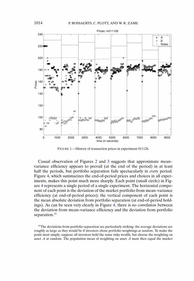
Figures 1, 2, and 3 summarize the results from a typical experiment.17 Fig-ure 1 shows the complete history of prices. Note that all transaction prices arebelow expected payoffs, reflecting the presence of substantial risk aversion.(Expected payoffs for asset A are the higher horizontal lines in each periodand expected payoffs for asset B are the lower horizontal lines. Because stateswere drawn without replacement, expected payoffs are not constant across pe-riods.) Figure 2 shows, with respect to prices at each transaction, the deviationof the market portfolio from mean–variance efficiency. Note that within eachperiod and over the course of the experiment, pricing comes to more closelyapproximate mean–variance pricing. Figure 3 shows individual portfolio hold-ings at the end of each period. Note that holdings appear quite random (subjectto the accounting identity that holdings sum to the market portfolio).
17Again, a complete record of every transaction in every experiment is available at http://www.hss.caltech.edu/~pbs/BPZdata.
1014 P. BOSSAERTS, C. PLOTT, AND W. R. ZAME
FIGURE 1.—History of transaction prices in experiment 011126.
Casual observation of Figures 2 and 3 suggests that approximate mean–variance efficiency appears to prevail (at the end of the period) in at leasthalf the periods, but portfolio separation fails spectacularly in every period.Figure 4, which summarizes the end-of-period prices and choices in all exper-iments, makes this point much more sharply. Each point (small circle) in Fig-ure 4 represents a single period of a single experiment. The horizontal compo-nent of each point is the deviation of the market portfolio from mean–varianceefficiency (at end-of-period prices); the vertical component of each point isthe mean absolute deviation from portfolio separation (at end-of-period hold-ings). As can be seen very clearly in Figure 4, there is no correlation betweenthe deviation from mean–variance efficiency and the deviation from portfolioseparation.18
18The deviations from portfolio separation are particularly striking: the average deviations areroughly as large as they would be if investors chose portfolio weightings at random. To make thepoint most simply, suppose all investors hold the same risky wealth, but choose the weighting onasset A at random. The population mean of weighting on asset A must then equal the market

CHOICES IN FINANCIAL MARKETS 1015
FIGURE 2.—Deviation from mean–variance efficiency computed with respect to transactionprices in experiment 011126.
5. ECONOMETRIC RESULTS
5.1. Testing Strategy
The (asymptotic) distribution of the GMM statistic under the CAPM + εis noncentral χ2 with 1 degree of freedom (the number of risky assets minus1) and with unknown noncentrality parameter. Our test builds on this prop-erty. Specifically, we compute the GMM statistic for the 60+ periods (samples)across our experiments. These outcomes are then used to construct empiricaldistribution functions of the GMM statistic.
weighting on asset A, which is approximately 0.4 in many of our experiments. This will be thecase if weightings on asset A are drawn independently from the distribution
32λ[0�0�4] + 2
3λ[0�6�1]�
where λE denotes the restriction of Lebesgue measure to E ⊂ [0�1]. In that case, the mean ab-solute deviation will be only 0.24.

1016 P. BOSSAERTS, C. PLOTT, AND W. R. ZAME
FIGURE 3.—Individual end-of period portfolio holdings in experiment 011126.
We cannot readily aggregate the results over all periods or even across all pe-riods in a single experiment, because periods within a single experiment are notindependent (subject populations are the same), so the GMM statistics acrossperiods within an experiment are not independent. However, periods in differ-ent experiments are independent (because the subject populations of differentexperiments are disjoint). We therefore construct eight samples; the first sam-ple consists of the first periods of all experiments, the second sample consistsof the second periods of all experiments, and so forth. We then test whetherthe empirical distribution of GMM statistics is noncentral χ2 for each sample.(We use only the first eight periods because we have only a few experimentsthat last nine periods.)
We use both the Kolmogorov–Smirnov statistic and the Cramer–von Misesstatistic. The former uses the supremum of the deviations of the empirical dis-tribution function (of the GMM statistic) from a noncentral χ2 distributionfunction; the latter uses the density-weighted mean squares of these deviations.We estimate the noncentrality parameter from all the data (all periods in allexperiments) to minimize estimation error. Effectively, the noncentrality para-meter is estimated on the basis of a sample that is at least seven times as large

CHOICES IN FINANCIAL MARKETS 1017
FIGURE 4.—Plot of mean absolute deviations of subjects’ end-of-period holdings from CAPMpredictions against distances from CAPM pricing (absolute difference between market Sharperatio and maximal Sharpe ratio, based on last transaction prices) for all periods in all experiments.There is no correlation between distance from CAPM pricing (x axis) and violation of portfolioseparation (y axis).
as the samples on which we test whether the empirical distribution function ofthe GMM statistic is noncentral χ2.19
5.2. Test Results
Figure 5 depicts the empirical distribution of the logarithm of the GMM sta-tistic across all periods in our experiments. The smooth line is the distributionof the logarithm of a central χ2-distributed random variable; the jagged line isthe empirical distribution of our test statistic. As can be seen, the jagged lineappears to be a horizontal translation of the smooth line, which suggests thatthe GMM statistics are drawn from a noncentral χ2 distribution. This sugges-tion is confirmed in Table IV, which reports the findings of the Kolmogorov–
19An alternative approach would be to estimate the in-sample noncentrality parameter and ad-just p values accordingly. We have not done this because the correct adjustments are not known.

1018 P. BOSSAERTS, C. PLOTT, AND W. R. ZAME
FIGURE 5.—Empirical distribution of the GMM statistic for all periods in all experiments(jagged line) against a central χ2 distribution (smooth line). A noncentral χ2 distribution providesa better fit, which is consistent with the small-sample biases expected if CAPM + ε is correct.
Smirnov (KS) and Cramer–von Mises (CvM) tests applied to our model. Foreach sample, we test the fit of the empirical distribution function of our GMMstatistics to a noncentral χ2 distribution using the best fit for the unknownnon-centrality parameter (11.6 for KS, 10.0 for CvM).20 In Table IV we followShorack and Wellner (1986, p. 239) to correct for small-sample biases; p val-ues are obtained from the same source. (Critical values for the Cramer–vonMises statistic are known only for some p values; for other p values, we reporta range.)
At the 1% level, both KS and CvM goodness-of-fit tests reject only in theperiod 2 sample, and do not reject in other period samples; i.e., they rejectin 12.5% of samples. At the 5% level, both KS and CvM reject only in theperiod 1 and 2 samples, and do not reject in other periods; i.e., they reject in
20Best fits are obtained as follows. Let FE(·) denote the empirical distribution function of theGMM statistic. Let Fλ2(·) denote the χ2 distribution with 1 degree of freedom and noncentralityparameter λ2. The best fit is obtained as
infλ2
supx
|FE(x)− Fλ2(x)|�

CHOICES IN FINANCIAL MARKETS 1019
TABLE IV
TESTS OF CAPM + ε ACCOMMODATING CORRELATION BETWEEN PRICES AND PERTURBATIONS
Period Number ofNumber Observations KSa p Valueb CvMc p Valueb
1 9 1.53 0�05 >p> 0�025 0.49 0�05 >p> 0�0252 9 2.01 p< 0�01 0.91 p< 0�013 9 1.01 p> 0�15 0.21 p> 0�154 9 1.33 0�15 >p> 0�10 0.30 0�15 >p> 0�105 8 1.26 0�10 >p> 0�05 0.21 p> 0�156 9 0.80 p> 0�15 0.21 0�10 >p> 0�057 6 0.87 p> 0�15 0.04 p> 0�158 4 1.26 0�10 >p> 0�05 0.42 0�10 >p> 0�05
aKolmogorov–Smirnov statistic of the difference between the empirical distribution function of GMM statisticsacross experiments for a fixed period and a noncentral χ2 distribution with noncentrality parameter 11.6. The KSstatistic is modified for small sample bias. See Shorack and Wellner (1986, p. 239).
bBased on Table 1 on page 239 of Shorack and Wellner (1986).cCramer–von Mises statistic of the difference between the empirical distribution function of GMM statistics across
experiments for a fixed period and a noncentral χ2 distribution with noncentrality parameter 10.0. The CvM statisticis modified for small sample bias. See Shorack and Wellner (1986, p. 239).
25% of samples. It might be useful to keep in mind that econometric tests ofasset-pricing models against historical data frequently reject at much smallervalues of p, and that our tests are more demanding because they test pricesand holdings. For example, in arguing that the performance of the three-factormodel is superior to other models, despite the fact that it is rejected at the0�5% significance level, Davis, Fama, and French (2002, p. 450) write:
. . . The three-factor model. . . is rejected by the. . . test. This result shows that the three-factor model is just a model and thus an incomplete description of expected returns. Whatthe remaining tests say is that the model’s shortcomings are just not those predicted by thecharacteristics model.
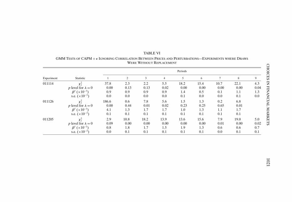
We have argued that the correlation between prices and perturbations in-herent in CAPM + ε means that the correct comparison of the distributionof our test statistic is with a noncentral χ2 distribution. Tables V and VI showthe result of ignoring this correlation and comparing the distribution of our teststatistic with a central χ2 distribution. (We separate experiments in which stateswere drawn with replacement from experiments where states were drawn with-out replacement only, because a combined table would be too large to displaylegibly on a single page.)
5.3. Power
There are several reasons to believe our tests have substantial power.(i) We require the noncentrality parameter to be the same across periods as
well as across experimental sessions. Because distributional properties of the in-

1020P.B
OSSA
ER
TS,C
.PLO
TT,A
ND
W.R
.ZA
ME
TABLE V
GMM TESTS OF CAPM + ε IGNORING CORRELATION BETWEEN PRICES AND PERTURBATIONS—EXPERIMENTS WHEREDRAWS WERE INDEPENDENTa
Periods
Experiment Statistic 1 2 3 4 5 6 7 8 9
981007 χ21 36�2 2�2 79�3 28�9 21�0 12�6
p level for λ= 0 0�00 0�14 0�00 0�00 0�00 0�00βI (×10−3) 0�8 0�7 1�3 1�1 1�3 1�1s.e. (×10−3) 0�0 0�1 0�0 0�1 0�0 0�0
981116 χ21 23�7 0�9 1�0 4�4 3�5 30�3
p level for λ= 0 0�00 0�35 0�32 0�04 0�06 0�00βI (×10−3) 1�5 1�1 0�8 1�0 1�9 2�0s.e. (×10−3) 0�1 0�1 0�1 0�1 0�1 0�1
990211 χ21 5�3 11�2 5�5 33�3 4�0 15�4 0�2
p level for λ= 0 0�02 0�00 0�02 0�00 0�04 0�00 0�69βI (×10−3) 1�1 1�5 1�4 2�8 1�2 1�5 −0�2s.e. (×10−3) 0�1 0�1 0�1 ∗ 0�1 0�1 0�1
990407 χ21 7�5 0�6 12�5 103�1 † 0�2 13�6 †
p level for λ= 0 0�02 0�44 0�00 0�00 — 0�66 0�00 —βI (×10−3) 0�5 0�5 0�3 −0�3 — 0�3 0�2 —s.e. (×10−3) 0�0 0�0 0�0 0�1 — 0�1 0�1 —
991110 χ21 197�5 72�8 31�6 7�4 2�7 6�9
p level for λ= 0 0�00 0�00 0�00 0�01 0�10 0�01βI (×10−3) 3�0 2�4 1�9 1�2 1�1 1�4s.e. (×10−3) * 0�1 0�1 0�1 0�1 0�1
991111 χ21 4�8 1�5 114�4 61�4 36�3 43�4 31�6 30�8
p level for λ= 0 0�03 0�23 0�00 0�00 0�00 0�00 0�00 0�00βI (×10−3) 0�4 0�3 1�7 1�4 1�2 1�0 1�3 1�3s.e. (×10−3) 0�0 0�1 * 0�0 0�0 0�0 0�0 0�0
aThe asterix (*) denotes that the weighting matrix was not positive definite and, hence, standard errors could not be computed. The dagger (†) denotes negative χ2 becauseweighting matrix was not positive definite.
CH
OIC
ES
INF
INA
NC
IAL
MA
RK
ET
S1021
TABLE VI
GMM TESTS OF CAPM + ε IGNORING CORRELATION BETWEEN PRICES AND PERTURBATIONS—EXPERIMENTS WHERE DRAWSWERE WITHOUT REPLACEMENT
Periods
Experiment Statistic 1 2 3 4 5 6 7 8 9
011114 χ21 37�8 2�3 2�2 5�5 18�2 15�4 10�7 22�1 4�3
p level for λ = 0 0�00 0�13 0�13 0�02 0�00 0�00 0�00 0�00 0�04βI (×10−3) 0�9 0�9 0�9 0�9 1�4 0�5 0�1 1�1 1�3s.e. (×10−3) 0�0 0�0 0�0 0�0 0�1 0�0 0�0 0�1 0�0
011126 χ21 186�6 0�6 7�8 5�6 1�5 1�3 0�2 6�8
p level for λ = 0 0�00 0�44 0�01 0�02 0�23 0�25 0�65 0�01βI (×10−3) 4�1 1�3 1�7 1�7 1�0 1�3 1�1 1�7s.e. (×10−3) 0�1 0�1 0�1 0�1 0�1 0�1 0�1 0�1
011205 χ21 2�9 10�8 18�2 13�9 13�6 15�6 7�9 19�0 5�0
p level for λ = 0 0�09 0�00 0�00 0�00 0�00 0�00 0�01 0�00 0�02βI (×10−3) 0�8 1�8 1�7 1�5 1�9 1�3 0�6 0�6 0�7s.e. (×10−3) 0�0 0�1 0�1 0�1 0�1 0�1 0�0 0�1 0�1

1022 P. BOSSAERTS, C. PLOTT, AND W. R. ZAME
dividual perturbation terms ultimately determine the value of the noncentralityparameter, this means that we implicitly assume that these properties do notchange across experiments. In other words, we impose a strong homogeneityassumption across different subject populations.
(ii) The noncentrality parameter imposes a tight relationship between the mo-ments of the GMM statistic. In particular, the difference between its varianceand its mean is equal to the (fixed) number of degrees of freedom plus threetimes the noncentrality parameter.
Formal analyses of power (or size) are often accomplished by means ofMonte Carlo analysis. In such analysis, values are posited for all the parametersof one’s economic model—in particular, for the parameters that determine thedistributions of the random variables—and draws from these distributions areused to generate a sequence of samples of a size comparable to the size of theactual sample(s) in the empirical study. The sequence of samples induces a se-quence of statistics with which one can construct a distribution—an estimateof the finite-sample distribution under the maintained parametric assumptions.Typically this exercise is conducted under a parameterization for which the nullhypothesis is satisfied, which provides an estimate of the true size of one’s test(true probability of rejecting a correct null based on the actual cutoffs used inthe empirical test), and then again under various parameterizations for whichthe null hypothesis is violated, so as to trace a power function (the probabilityof rejecting the null when it is false, as a function of changes in such parame-terizations).
In our context, however, Monte Carlo power analysis seems both infeasibleand arbitrary.• Monte Carlo analysis seems infeasible in our setting because the relevant
parameter space is infinite dimensional. In our context, the relevant parame-ters are the distributions of endowments, mean–variance demand functions,and perturbations. Endowments and mean–variance demand functions aredetermined by four real parameters, but perturbations are functions of un-known form. Hence, the perturbations are specified by a distribution onan infinite-dimensional function space. One might restrict attention to aparticular class of perturbation functions, but we have no idea what classcould/should be used.
• Monte Carlo seems arbitrary in our setting because power analysis requiresspecification of plausible parameterizations for which the null hypothesis isviolated. In our setting, there are many ways in which the null hypothesiscould be violated, and it is not at all obvious what possible violations shouldbe thought most relevant. Obvious choices include the possibility that per-turbation functions are not drawn independently, that they are not drawnfrom a distribution with mean zero, or that the market is not in equilibriumat the end of each experimental period.One might respond to these objections by using the data to suggest para-
meterizations and relevant violations of the null hypothesis. However, a much

CHOICES IN FINANCIAL MARKETS 1023
TABLE VII
POWER ANALYSIS: TESTS OF CAPM + ε ACCOMMODATING CORRELATION BETWEEN PRICESAND PERTURBATIONS WHEN PERTURBING PRICES BY 5 FRANCS IN THREE
RANDOMLY CHOSEN EXPERIMENTS
Period Number ofNumber Observations KSa p Valueb CvMc p Valueb
1 9 1.49 0�025 >p> 0�01 1.15 p< 0�012 9 2.12 p< 0�01 0.79 p< 0�013 9 1.52 0�025 >p> 0�01 0.44 0�10 >p> 0�054 9 0.75 p> 0�15 0.12 p> 0�155 8 1.33 0�10 >p> 0�05 0.11 p> 0�156 9 1.04 p> 0�15 0.23 p> 0�157 6 1.31 0�10 >p> 0�05 0.46 0�05 >p> 0�0258 4 1.52 0�025 >p> 0�01 0.60 0�025 >p> 0�01
aKolmogorov–Smirnov statistic of the difference between the empirical distribution function of GMM statisticsacross experiments for a fixed period and a noncentral χ2 distribution with noncentrality parameter 30.3. The KSstatistic is modified for small sample bias. See Shorack and Wellner (1986, p. 239).
bBased on Table 1 on page 239 of Shorack and Wellner (1986).cCramer–von Mises statistic of the difference between the empirical distribution function of GMM statistics across
experiments for a fixed period and a noncentral χ2 distribution with noncentrality parameter 25.0. The CvM statisticis modified for small sample bias. See Shorack and Wellner (1986, p. 239).
more straightforward approach to power analysis is available. Monte Carloanalysis is most useful when one does not have data, but we do have data,which is generated by actual economies. It seems more natural, therefore, touse the data we have to generate tests of power.21
Motivated by this reasoning, we offer two tests of power generated with theexisting data:• In the theory, choices determine prices. Our test does not reject the theory;
that is, data appear to be consistent with the theory. Asking for the power ofthe test amounts to asking whether the tests would have rejected the theoryon other data. To answer this question, we systematically perturb prices in threerandomly chosen experiments. The new prices are within 5 francs (2.5%) ofthe prices found in the experiments: higher prices for security A and lowerprices for security B. In comparison to the range of prices we observe inour experiments—both across experiments and within a single experiment—this is a marginal change in prices. To put it in statistical terms, we say theunconditional probability (i.e., the probability not conditional on subjects’actual choices) of observing such prices is high. As can be seen in Table VII,if we apply our tests to the artificial data (perturbed prices, same choices),we reject the theory at the 5% level in 50% of all samples for both the KS
21Of course, the use of one’s own data also underlies bootstrap estimation, which has largelyreplaced Monte Carlo analysis to estimate the correct size of one’s test under the null hypothesis.

1024 P. BOSSAERTS, C. PLOTT, AND W. R. ZAME
and CvM tests, whereas on the actual data we reject at the 5% level in only25% of all samples. Put differently, the theory would be strongly rejected ifas few as 1/3 of the prices differed from actual prices by as little as 2.5%; thisprovides an indirect demonstration of substantial power. One cannot explainactual choices by prices that are only slightly different, even if those pricesare likely to be observed in other periods. Thus, there is something specialabout the prices in a given period: they match the choices in that period andonly in that period.22
• Our second exercise investigates power against violations of the statisticalassumption that economies are drawn independently. To assure indepen-dence, we used samples that consist of the outcomes (prices, choices) in a(fixed) period across all experiments. This guarantees independence becausesubject populations are disjoint across experiments. If, instead, we used out-comes from all periods of a given experiment, we would then have samplesthat fail the assumption of independence, because subject populations areconstant within a single experiment, whence choices within an experiment,which determine prices, are presumably correlated as well. When we applyour goodness-of-fit tests to these experimentwise samples, our p values godown significantly and we reject more often. As Table VIII shows, at the 5%level the KS test now rejects 44% of the time and the CvM test rejects 33%of the time. The decrease in p values and increase in number of rejectionsdemonstrate power for purely statistical violations of our null hypothesis.
6. CONCLUSION
In this paper, we provide a rationale for testing asset-pricing models that relyon portfolio separation (such as CAPM and its multifactor extensions) even inthe absence of convincing evidence for such portfolio separation. We offer atheoretical model, a novel econometric procedure to test the model, and testsbased on data from experimental financial markets. These tests fail to rejectthe model.
Our analysis suggests several lessons. The first is that, despite the modestrisks, experimental financial markets can provide significant and useful in-sights. A second is that the standard model of choice under unobserved het-erogeneity that is widely used in applied economics should be used with somecare. In finite markets, unexplained heterogeneity in demands (usually a keydeterminant of the unexplained portion of observed choices) need not be or-thogonal to prices, and this may have significant effects on the econometricanalysis.
22An alternative would have been to systematically perturb prices in all experiments. How-ever, in that case we would have changed the entire (unconditional) distribution of prices, andthe distribution would not have been the one obtained in the experiments. Hence, such a priceperturbation seems to be beside the point. We think that our exercise is the right one.

CHOICES IN FINANCIAL MARKETS 1025
TABLE VIII
POWER ANALYSIS: TESTS OF CAPM + ε ACCOMMODATING CORRELATION BETWEEN PRICESAND PERTURBATIONS—TESTS PER EXPERIMENT (VIOLATING INDEPENDENCE)
Experiment Number ofNumber Observations KSa p Valueb CvMc p Valueb
981007 6 1.43 0�05 >p> 0�025 0.70 0�025 >p> 0�01981116 6 1.50 0�025 >p> 0�01 0.41 0�10 >p> 0�05990211 7 1.20 0�15 >p> 0�10 0.10 p> 0�15990407 6 0.86 p> 0�15 0.04 p> 0�15991110 6 1.27 0�10 >p> 0�05 0.23 p> 0�15991111 8 2.19 p< 0�01 1.19 p< 0�01011114 9 0.95 p> 0�15 0.10 p> 0�15011126 8 1.81 p< 0�01 0.83 p< 0�01011205 9 0.54 p> 0�15 0.06 p> 0�15
aKolmogorov–Smirnov statistic of the difference between the empirical distribution function of GMM statisticsacross experiments for a fixed period and a noncentral χ2 distribution with noncentrality parameter 11.6. The KSstatistic is modified for small sample bias. See Shorack and Wellner (1986, p. 239).
bBased on Table 1 on page 239 of Shorack and Wellner (1986).cCramer–von Mises (CvM) statistic of the difference between the empirical distribution function of GMM statistics
across experiments for a fixed period and a noncentral χ2 distribution with noncentrality parameter 10.0. The CvMstatistic is modified for small sample bias. See Shorack and Wellner (1986, p. 239).
In contrast to standard econometric analysis, the econometric procedure in-troduced here explicitly links prices and choices. We have applied this proce-dure only to data from experimental financial markets, but it is applicable tohistorical data as well, provided suitable choice data can be found.
Division of the Humanities and Social Sciences, California Institute of Tech-nology, Baxter Hall, 1200 E. California Blvd., Pasadena, CA 91125, U.S.A., andCenter for Economic Policy Research, London, U.K., and Swiss Finance Institute,Zurich, Switzerland; [email protected],
Division of the Humanities and Social Sciences, California Institute of Tech-nology, Baxter Hall, 1200 E. California Blvd., Pasadena, CA 91125, U.S.A.;[email protected],
andDept. of Economics, University of California, Los Angeles, Bunche Hall, Los
Angeles, CA 90095, U.S.A., and California Institute of Technology, Pasadena, CA91125, U.S.A.; [email protected].
Manuscript received July, 2003; final revision received March, 2007.
APPENDIX A: CAPM
To derive the conclusions of CAPM in our setting in which short sales ofrisky assets are not permitted, we begin by analyzing the setting in which arbi-trary short sales are permitted. Write Zi(p), respectively zi(p), for investor i’s

1026 P. BOSSAERTS, C. PLOTT, AND W. R. ZAME
demand for all assets, respectively risky assets, when the price of risky assetsis p. Note that either of Zi(p) or zi(p) determines the other (through budgetbalance). We will focus on whichever is convenient for the purpose at hand.
Assuming, as we do throughout, that consumptions are in the range wherepreferences are monotone, the first-order conditions for optimality and somealgebra show that
zi(p)= 1bi∆−1(µ−p)�(15)
At equilibrium, the demands for risky assets must clear the market for riskyassets, so if p is an equilibrium price, then
I∑i=1
zi(p) =m�
From these equations we can solve for the unique equilibrium price p:
p= µ−(
I∑i=1
1bi
)−1
∆m= µ−(
1I
I∑i=1
1bi
)−1
∆m�
In our setting, short sales of risky assets are not permitted and demand func-tions are not given by the equation (15). However, we assert that the modelwith short sales and our model without short sales admit the same equilibriumprices.
To see this, write zi(p) for investor i’s demand for risky assets when pricesare p and short sales of risky assets are not permitted. Note that zi(p)= zi(p)whenever zi(p) ≥ 0: in particular, zi(p) = zi(p). It follows immediately thatp is an equilibrium price in the setting when short sales of risky assets arenot permitted. To see that there is no other equilibrium price in this setting,suppose that p∗ �= p were such an equilibrium price. If constrained demandzj(p∗) were strictly positive for some investor j, then constrained demandzj(p∗) would coincide with unconstrained demand zj(p∗) for investor j. How-ever, formula (15) guarantees that if zj(p∗) were positive for some investor j,then zi(p∗) would be positive for every investor i, whence zi(p∗) would coin-cide with zi(p∗) for every investor i. Because p∗ �= p, this would imply thatp∗ was not an equilibrium price after all. It follows that constrained demandzj(p∗) cannot be strictly positive for any investor j. At equilibrium, asset mar-kets clear. Because the market portfolio is strictly positive, it follows that someinvestor k chooses an equilibrium portfolio that involves the risky asset A butnot the risky asset B, and some investor � chooses an equilibrium portfolio thatinvolves the risky asset B but not the risky asset A:
zkA(p
∗) > 0� zkB(p
∗)= 0�
z�A(p
∗)= 0� z�B(p
∗) > 0�

CHOICES IN FINANCIAL MARKETS 1027
The first-order conditions for investors k and � entail
p∗A
p∗B
≤ MUkA
MUkB
�
p∗B
p∗A
≤ MU�B
MU�A
�
Direct calculation using the explicit form of utility functions and making use ofthe fact that var(x+ y)= var(x)+ 2 cov(x� y)+ var(y) yields
MUkA
MUkB
= E(A)− bkzkA(p
∗) var(A)
E(B)− bkzkA(p
∗) cov(A�B)�
MU�B
MU�A
= E(B)− b�z�B(p
∗) var(B)E(A)− bkzk
B(p∗) cov(A�B)
�
Our assumptions guarantee that bk�b�� var(A)� and var(B) are all strictly pos-itive, and the particular structure of payoffs of the risky assets and the stateprobabilities guarantee that cov(A�B) < 0. Combining all these yields
p∗A
p∗B
≤ MUkA
MUkB
< 1�
p∗B
p∗A
≤ MU�B
MU�A
< 1�
This is a contradiction, so we conclude that p is the unique equilibrium price,as asserted.
APPENDIX B: CAPM + ε
In this appendix we give a formal and rigorous presentation of the idea of thetrue economy as draw from a distribution of individual characteristics and as aperturbation of a mean–variance economy. Although the ideas are simple, andthe conclusions are both intuitive and expected, the details require a little care.As we shall see, the analysis depends on the fact that cov(A�B) < 0 (whichguarantees that the equilibria of the ideal economy with short sales and withoutshort sales are the same) and on the fact that the CAPM equilibrium of theideal economy is regular (which guarantees that the perturbed economy hasan equilibrium near the CAPM equilibrium of the ideal economy).
We work throughout in the setting of Section 2 and Appendix A, and retainthe same notation. In particular, two risky assets and one riskless asset aretraded. The risky assets cannot be sold short, but the riskless asset can be.The covariance of the risky assets is negative; consumption may be negative.

1028 P. BOSSAERTS, C. PLOTT, AND W. R. ZAME
We normalize throughout so that the price of the riskless asset is 1; the vectorof asset prices is q = (p�1) ∈ R
3++. As before, we write µ for the vector of
expected returns on risky assets and write ∆ for the covariance matrix of riskyassets.
B.1. Distributions and Draws from a Distribution
We follow Hart, Hildenbrand, and Kohlberg (1974) in describing economiesas distributions on the space of investor characteristics. The usual descriptionof an investor is in terms of an endowment bundle of commodities and pref-erences over commodity bundles, but we find it more convenient to adopt adescription in terms of an endowment portfolio of assets and a demand func-tion for assets. We assume that endowments and prices, hence wealth, lie ingiven compact sets End ⊂ R
2+ × R, P ⊂ R
3++, and [0�w] ⊂ R+. An investor is
characterized by an endowment ω ∈ End of riskless and risky assets, and by acontinuous demand function
Z :P × [0�w] → R2+ × R
for risky and riskless assets as a function of wealth w ∈ [0�w] ⊂ R+ and pricesfor risky assets p ∈P ⊂ R
2++. (Recall that we have normalized so that the price
of the riskless asset is 1.) We assume throughout that the value of demand isequal to the value of the endowment, that is
(p�1) ·Z(p� (p�1) ·ω)= (p�1) ·ω ≤ [0�w]for each ω�p. (We could assume that demand satisfies properties that followfrom revealed preference, but there is no need to do so.) Write D for the spaceof demand functions and equip D with the topology of uniform convergence.Then End ×D is the space of investor characteristics.
We view a compactly supported probability measure τ on End × D as thedistribution of investor characteristics in a fixed economy and also as the dis-tribution of characteristics of the pool from which economies are drawn. Givenan integer I, a particular draw of I investors from τ can be described by a dis-tribution of the form
τ = 1I
I∑i=1
δ(ωi�Zi)�
where δ(ωi�Zi) is point mass at the characteristic (ωi�Zi) ∈ suppτ ⊂ End × D.We identify the set of such draws with (suppτ)I , which, by abuse of notation,we view as a subset of M(E×D), the space of all compactly supported proba-bility measures on End ×D. The I-fold product measure τI on (suppτ)I is thedistribution of all draws.

CHOICES IN FINANCIAL MARKETS 1029
B.2. Equilibrium
Given a distribution η ∈ M(E × D), an equilibrium for η is a price p ∈ Psuch that∫
Z(p� (p�1) ·ω)dη=∫
ωdη�
(Because we describe investor characteristics in terms of demand functions, wefocus on prices and suppress consumptions. Of course, Z(p� (p�1) · ω) is theequilibrium consumption of the investor with characteristics (ω�Z).)
We caution the reader that a distribution η need not admit an equilibriumand that convergence of distributions does not imply convergence of (sets of)equilibria. However, as we shall show, the situation is much better for the dis-tributions of most interest to us.
B.3. CAPM Distributions
Given an endowment ω, the portfolio θ is budget feasible if (p�1) ·θ ≤ (p�1) ·ω for every p ∈ P . We say σ ∈ M(End ×D) is a mean–variance distribution iffor each (ω�Z) ∈ suppσ there is a coefficient of risk aversion b(ω�Z) > 0such that the mean–variance utility function
Ub(ω�Z) =E(x)− 1b(ω�Z)
var(x)
is strictly monotone on the set of dividends of feasible portfolios and Z isthe (restriction of) the portfolio demand function derived from Ub(ω�Z). (Keepin mind that we require holdings of risky assets to be nonnegative.) Given amean–variance distribution σ , we write Bσ = ∫
b(ω�Z)−1 dσ for the marketrisk tolerance and mσ = ∫
ωdσ for the per capita market portfolio. We say themean–variance distribution σ is a CAPM distribution if the price
pσ = µ−B−1σ ∆mσ
belongs to intP , the interior of P . If σ is a CAPM distribution, it follows as inAppendix A that σ admits pσ as the unique equilibrium price, that the meanmarket portfolio m is mean–variance efficient at prices pσ , and that equilib-rium holdings of risky assets z(pσ� (pσ�1) · ω) are nonnegative multiples ofthe mean market portfolio m (portfolio separation).
B.4. Mean-Zero Perturbations
Write πE :E × D → E for the projection on the first factor. If τ�σ ∈M(E × D), we say τ is a perturbation of σ if there is a measurable functionf : suppτ →D such that σ = (πE� f )∗τ; that is,
σ(B)= τ((πE� f )−1(B))= τ
{(ω�Z) : (ω�f (ω�Z)) ∈ B
}

1030 P. BOSSAERTS, C. PLOTT, AND W. R. ZAME
for each Borel set B ⊂ E ×D. We say τ is a mean-zero perturbation of σ if, inaddition, ∫
[Z − f (ω�Z)]dτ =∫
Zdτ −∫
Z′ dσ = 0�
Evidently, if τ is a mean-zero perturbation of σ , then τ and σ admit the sameequilibria—although neither may admit any equilibrium at all.
B.5. Perturbations of CAPM Distributions
We are now in a position to state and prove the result we require.
THEOREM B.1: Let σ be a CAPM distribution and let τ be a mean-zero per-turbation of σ . For each ε0 > 0 there is an integer I0 and for every I > I0 there is asubset �I ⊂ (suppτ)I such that:
(i) τI(�I) > 1 − ε0;(ii) for every γ ∈ �I , the draw γ = F(γ) from σ admits a unique equilibrium
pγ and the draw γ from τ admits at least one equilibrium;(iii) if γ ∈ �I and pγ is any equilibrium of γ, then ‖pγ −pγ‖< ε0.
Informally, if we draw a large enough sample from τ, then, with high proba-bility the sample economy and the CAPM economy of which it is a perturbationhave nearly the same equilibrium price(s).
PROOF OF THEOREM B.1: If ν is a distribution, let Dν :P → R2+ × R be the
market demand function for assets:
Dν(p) =∫
Z(p� (p�1) ·ω)dν
and let Mν be the per capita market portfolio
Mν =∫
ωdν�
By definition, an equilibrium for ν is a zero of excess demand Dν −Mν .By assumption, pσ ∈ intP . Choose ε1 < ε0 so that B(pσ�ε1) ⊂ P . Direct
computation shows that the excess demand function Dσ −Mσ is regular at pσ .It follows that there is an ε2 > 0 such that if H :P → R
2+ × R is any continuous
function and
‖H − (Dσ −Mσ)‖B(pσ �ε1) < ε2�
then H has at least one zero in B(pσ�ε1).

CHOICES IN FINANCIAL MARKETS 1031
On the other hand, Dσ − Mσ is bounded away from 0 on P \ B(pσ�ε1), sothere is an ε3 > 0 such that if
‖H − (Dσ −Mσ)‖P\B(pσ �ε1) < ε3�
then H is bounded away from 0 on P \ B(pσ�ε1). Setting ε = min{ε1� ε2� ε3},we conclude that if H :P → R
2+ × R is any continuous function for which
‖H − (Dσ −Mσ)‖P < ε�
then H has at least one zero on P and all its zeroes belong to B(pσ�ε), andhence belong to B(pσ�ε0).
For each I, set
G1I = {γ ∈ (suppτ)I :‖Zγ −Zτ‖< ε/2}�
H1I = {γ ∈ (suppτ)I :‖Mγ −Mτ‖< ε/2}�
G2I = {ζ ∈ (suppσ)I :‖Zζ −Zτ‖ < ε/2}�
H2I = {ζ ∈ (suppσ)I :‖Mζ −Mσ‖ < ε/2}�
�I = G1I ∩H2
I ∩ F−1(G2I )∩ F−1(H2
I)�
Market demand is the expectation of individual demand and the per capitamarket portfolio is the expectation of individual endowment portfolios, so ap-plying the strong law of large numbers in the space of continuous functionsΦ :P → R
3 (see Ledoux and Talagrand (1991) for the appropriate Banachspace version) and in R
3 implies that there is an index I0 such that if I > I0,then
τI(G iI) > 1 − ε
4�
σI(HiI) > 1 − ε
4
for i = 1�2.Let f be the function given in the definition of mean-zero perturbation and
write F = (πE� f ). By assumption
τ(F−1(G2I ))= σ(G2
I ) and τ(F−1(H2I))= σ(H2
I)�
so if I > I0, then τ(�I) > 1 − ε.Finally, if γ ∈ GI , then
‖(Dγ −Mγ)− (Zγ −Mγ)‖ < ε�
‖(DF∗γ −MF∗γ)− (Zσ −Mσ)‖ < ε�

1032 P. BOSSAERTS, C. PLOTT, AND W. R. ZAME
Our construction guarantees that γ and F∗γ each admit at least one equilib-rium and that all these equilibria lie in B(pσ�ε0). Finally, because F∗γ is aCAPM economy, it actually admits a unique equilibrium, so the proof is com-plete. Q.E.D.
APPENDIX C: ESTIMATION OF W
We first specify our estimator ΞI of W . After that, we provide an asymptot-ically unbiased and uncorrelated estimator of individual risk tolerances to beused in the formulation of W . Third, we prove that the error of this estimatordoes not affect the asymptotic properties of ΞI . As a result, we substitute truerisk tolerances for estimates of the risk tolerances in the formula of ΞI and weproceed to the fourth step, where we prove convergence of ΞI to W .
In the sequel, we take the risk aversion coefficients as fixed. This is consistentwith the theory as long as perturbations are drawn independently from riskaversion coefficients. The econometrics conditions on risk aversion.
Likewise, we assume that individual perturbations are independent acrossperiods within an experimental session. In fact, all we need is that they areasymptotically orthogonal conditional on prices:
E{[εit]k[εiτ]j|pN1 � � � � �p
It } → 0(16)
for all τ �= t, as N → ∞.
C.1. The Estimator ΞI
To understand our estimator ΞI of W , let βit denote agent i’s risk tolerance,
that is, βit = 1/bi
t . Define the cross-sectional average holding: Let
mI = 1I
I∑i=1
zit �(17)
Also define
W I = IE[hIt (B
It )h
It (B
It )
T|pIt ]�
So W is the limit of W I as I → ∞. Now reformulate W I :
W I = IE[hIt (B
It )h
It (B
It )
T|pIt ] = (BI
t )2 1I
I∑i=1
E[εitεitT|pIt ]
= (BIt )
2 1I
I∑i=1
E[(εit +βi
t∆−1(µ−pI
t )−mI)
× (εit +βit∆
−1(µ−pIt )−mI)T|pI
t
]

CHOICES IN FINANCIAL MARKETS 1033
− 12(BI
t )2 1I
I∑i=1
E[(εit +βi
t∆−1(µ−pI
t )−mI)
× (E[zit |pI
t ] −mI)T|pIt
]− 1
2(BI
t )2 1I
I∑i=1
E[(βi
t∆−1(µ−pI
t )−mI)
× (εit +βit∆
−1(µ−pIt )−mI)T|pI
t
]− 1
2(BI
t )2 1I
I∑i=1
E[εit(β
it∆
−1(µ−pIt )−mI)T|pI
t
]− 1
2(BI
t )2 1I
I∑i=1
E[(βi
t∆−1(µ−pI
t )−mI)εitT|pI
t
]= (BI
t )2 1I
I∑i=1
E[(zit −mI)(zi
t −mI)T|pIt ]
− 12(BI
t )2 1I
I∑i=1
E[(zi
t −mI)(βit∆
−1(µ−pIt )−mI)T|pI
t
]− 1
2(BI
t )2 1I
I∑i=1
E[(βi
t∆−1(µ−pI
t )−mI)(zit −mI)T|pI
t
]− 1
2(BI
t )2 1I
I∑i=1
E[εit(β
it∆
−1(µ−pIt )−mI)T|pI
t
]− 1
2(BI
t )2 1I
I∑i=1
E[(βi
t∆−1(µ−pI
t )−mI)εitT|pI
t
]�
where the last equality follows from
εit = zit −βi
t∆−1(µ−pI
t )�
Now consider
mI − 1I
I∑i=1
βit∆
−1(µ−pIt ) = 1
I
I∑i=1
(zit −βi
t∆−1(µ−pI
t ))
= 1I
I∑i=1
εit�

1034 P. BOSSAERTS, C. PLOTT, AND W. R. ZAME
which converges to zero by the law of large numbers. As a result, the second-to-last term of the above expression becomes
12(BI
t )2 1I
I∑i=1
E[εit(β
it∆
−1(µ−pIt )−mI)T|pI
t
]= 1
2(BI
t )2 1I
×I∑
i=1
E
[εit
(βi
t∆−1(µ−pI
t )− 1I
I∑ν=1
βνt ∆
−1(µ−pIt )
)T∣∣∣pIt
]�
which converges to zero, because E[εit|pIt ] → 0.23 The same applies to the last
term in the above expression.We shall make the same substitution for mI in the second and third terms.
Consequently, there is no difference asymptotically if we define W I as
W I = (BIt )
2 1I
I∑i=1
E[(zit −mI)(zi
t −mI)T|pIt ]
− 12(BI
t )2 1I
×I∑
i=1
E
[(zi
t −mI)
([βi
t −1I
I∑ν=1
βνt
]∆−1(µ−pI
t )
)T∣∣∣pIt
]
− 12(BI
t )2 1I
×I∑
i=1
E
[([βi
t −1I
I∑ν=1
βνt
]∆−1(µ−pI
t )
)(zi
t −mI)T∣∣∣pI
t
]�
Note that this expression does not involve unobservables, except for the risktolerances βi
t , which we will discuss below.This suggests the following estimator. Define the cross-sectional covariance
of choices
cov(zit)= 1
I
I∑i=1
(zit −mI)(zi
t −mI)T�
23We have that√NE[εit |pI
t ] → λ, so a fortiori, E[εit |pIt ] → 0.
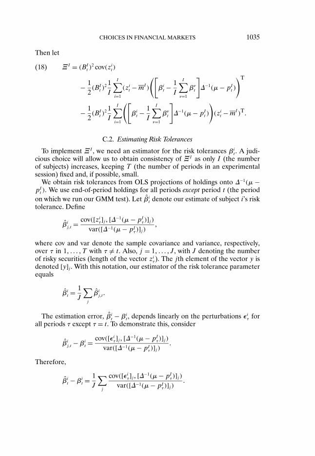
CHOICES IN FINANCIAL MARKETS 1035
Then let
ΞI = (BIt )
2 cov(zit)(18)
− 12(BI
t )2 1I
I∑i=1
(zit −mI)
([βi
t −1I
I∑ν=1
βνt
]∆−1(µ−pI
t )
)T
− 12(BI
t )2 1I
I∑i=1
([βi
t −1I
I∑ν=1
βνt
]∆−1(µ−pI
t )
)(zi
t −mI)T�
C.2. Estimating Risk Tolerances
To implement ΞI , we need an estimator for the risk tolerances βit . A judi-
cious choice will allow us to obtain consistency of ΞI as only I (the numberof subjects) increases, keeping T (the number of periods in an experimentalsession) fixed and, if possible, small.
We obtain risk tolerances from OLS projections of holdings onto ∆−1(µ −pI
t ). We use end-of-period holdings for all periods except period t (the periodon which we run our GMM test). Let βi
t denote our estimate of subject i’s risktolerance. Define
βij�t =
cov([ziτ]j� [∆−1(µ−pI
τ)]j)var([∆−1(µ−pI
τ)]j)�
where cov and var denote the sample covariance and variance, respectively,over τ in 1� � � � �T with τ �= t. Also, j = 1� � � � � J, with J denoting the numberof risky securities (length of the vector zi
τ). The jth element of the vector y isdenoted [y]j . With this notation, our estimator of the risk tolerance parameterequals
βit =
1J
∑j
βij�t �
The estimation error, βit − βi
t , depends linearly on the perturbations εiτ forall periods τ except τ = t. To demonstrate this, consider
βij�t −βi
t =cov([εiτ]j� [∆−1(µ−pI
τ)]j)var([∆−1(µ−pI
τ)]j)�
Therefore,
βit −βi
t =1J
∑j
cov([εiτ]j� [∆−1(µ−pIτ)]j)
var([∆−1(µ−pIτ)]j)
�

1036 P. BOSSAERTS, C. PLOTT, AND W. R. ZAME
The sample covariances in the last expression are linear in the perturbations[εiτ]j . It follows that the estimation error βi
t − βit is linear in the perturbations
[εiτ]j .Linearity implies that our estimator will be unbiased asymptotically because
E[εit|pIt ] → 0 (see footnote 23); hence E[βi
t −βit |pN
1 � � � � �pIt ] → 0.
Also, linearity together with the assumed asymptotic conditional time seriesorthogonality of individual perturbations implies that the estimation error βi
t −βi
t is uncorrelated with εit :
E{[εit]k(βit −βi
t)|pI1� � � � �p
IT }
= 1J
∑j
cov(E{[εit]k[εiτ]j|pI1� � � � �p
IT }� [∆−1(µ−pI
τ)]j)var([∆−1(µ−pI
τ)]j)→ 0
for all k (k= 1� � � � � J).
C.3. The Impact of Estimation Error in Risk Tolerances
To demonstrate that the errors in estimating risk tolerances have no effecton ΞI asymptotically, first consider the leading factor in the definition of ΞI ,namely, (BI
t )2. Because individual risk tolerances are estimated in an unbiased
way,
1I
I∑i=1
βit −
1I
I∑i=1
1bit
→ 0�
by the law of large numbers, so estimation error in the leading factor can beignored asymptotically.
Ignoring the leading factor, consider next the second term in the formula forΞI . (The argument for the third term is analogous and will not be presented.)Rewrite it in terms of the true risk tolerances plus estimation errors:
1I
I∑i=1
(zit −mI)
([βi
t −1I
I∑ν=1
βνt
]∆−1(µ−pI
t )
)T
= 1I
I∑i=1
(zit −mI)
([βi
t −1I
I∑ν=1
βνt
]∆−1(µ−pI
t )
)T
+ 1I
I∑i=1
(zit −mI)
CHOICES IN FINANCIAL MARKETS 1037
×([
(βit −βi
t)− 1I
I∑ν=1
(βνt −βν
t )
]∆−1(µ−pI
t )
)T
�
Consider the deviations of portfolio choices from the grand mean in the secondterm of the last expression, zi
t −mI , i = 1� � � � � I. These depend linearly on theperturbations εit , i = 1� � � � � I. In the same term, the estimation errors, namelyβi
t − βit and βν
t − βνt , are asymptotically mean zero. They are also asymptoti-
cally uncorrelated with the perturbations εit , because they depend linearly onperturbations εiτ for τ �= t, as demonstrated earlier. Clearly, the second term inthe above expression is simply the sample covariance of linear transformationsof perturbations εiτ for τ �= t, on the one hand, and linear transformations ofthe perturbations εit , on the other hand. Asymptotically, this sample covarianceconverges to zero in expectation. Because perturbations εiτ and εit are assumedto be independent across i, the law of large numbers implies that the samplecovariance will converge to its expectation. Consequently, the second term inthe above expression is zero asymptotically.
This leaves us only with the first term in curly brackets. The random behaviorof the first term obviously does not depend on errors in the estimation of therisk tolerances. We have the desired result: asymptotically, estimation errorshave no impact on ΞI .
C.4. Consistency of ΞI
Because their estimation errors have no effect asymptotically, we can writeΞI as a function of the true risk tolerances. This is what we did in (18). Con-vergence to W I , and hence A, is immediate.
REFERENCES
ARROW, K., AND F. HAHN (1971): General Competitive Analysis. San Francisco: Holden-Day.[1010]
ASPAROUHOVA, E., P. BOSSAERTS, AND C. PLOTT (2003): “Excess Demand and Equilibration inMulti-Security Financial Markets: The Empirical Evidence,” Journal of Financial Markets, 6,1–22. [996]
BOSSAERTS, P., AND C. PLOTT (2001): “The CAPM in Thin Experimental Financial Markets,”Journal of Economic Dynamics and Control, 26, 1093–1112. [1001]
(2004): “Basic Principles of Asset Pricing Theory: Evidence from Large-Scale Experi-mental Financial Markets,” Review of Finance, 8, 135–169. [996]
BOSSAERTS, P., C. PLOTT, AND W. ZAME (2002): “Discrepancies Between Observed and Theoret-ical Choices in Financial Markets Experiments: Subjects’ Mistakes or the Theory’s Mistakes?”Working Paper, Caltech. [997]
CONNOR, G. (1984): “A Unified Beta Pricing Theory,” Journal of Economic Theory, 34, 13–31.[993]
DAVIS, J., E. FAMA, AND K. FRENCH (2002): “Characteristics, Covariances, and Average Returns:1929 to 1997,” Journal of Finance, 55, 389–406. [993,1019]
GIBBONS, M., S. ROSS, AND J. SHANKEN (1989): “A Test of the Efficiency of a Given Portfolio,”Econometrica, 57, 1121–1152. [1010]

1038 P. BOSSAERTS, C. PLOTT, AND W. R. ZAME
HART, S., W. HILDENBRAND, AND E. KOHLBERG (1974): “Equilibrium Allocations as Distribu-tions on the Commodity Space,” Journal of Mathematical Economics, 1, 159–166. [1028]
HOLT, C., AND S. LAURY (2002): “Risk Aversion and Incentive Effects,” American EconomicReview, 92, 1644–1655. [999,1010]
JUDD, K., AND S. GUU (2001): “Asymptotic Methods for Asset Market Equilibrium Analysis,”Economic Theory, 18, 127–157. [994,998]
LEDOUX, M., AND M. TALAGRAND (1991): Probability in Banach Spaces. New York: Springer-Verlag. [1031]
MCFADDEN, D. (1989): “A Method of Simulated Moments for Estimation of Discrete ResponseModels Without Numerical Integration,” Econometrica, 57, 995–1026. [995,1002]
MERTON, R. C. (1973): “An Intertemporal Capital Asset Pricing Model,” Econometrica, 41,867–887. [993]
PAKES, A., AND D. POLLARD (1989): “Simulation and the Asymptotics of Optimization Estima-tors,” Econometrica, 57, 1027–1057. [995,1002]
RADNER, R. (1972): “Existence of Equilibrium of Plans, Prices, and Price Expectations in a Se-quence of Markets,” Econometrica, 40, 289–303. [1010]
ROLL, R. (1977): “A Critique of the Asset Pricing Theory’s Tests, Part I: On the Past and PotentialTestability of the Theory,” Journal of Financial Economics, 4, 129–176. [999]
SHARPE, W. (1964): “Capital Asset Prices: A Theory of Market Equilibrium under Conditions ofRisk,” Journal of Finance, 19, 425–442. [1010]
SHORACK, G. R., AND J. A. WELLNER (1986): Empirical Processes with Applications to Statistics.New York: Wiley. [1018,1019,1023,1025]