econometrics i: ols

Econometrics I: OLS

Dean Fantazzini

Dipartimento di Economia Politica e Metodi Quantitativi

University of Pavia

Overview of the Lecture

1st EViews Session I: Convergence in the Solow Model

Econometrics I: OLS

Dean Fantazzini2



2nd EViews Session II: Estimating a money demand equation

Econometrics I: OLS

Dean Fantazzini2-a



2nd EViews Session II: Estimating a money demand equation

3rd EViews Session III: Monte Carlo Simulation

Econometrics I: OLS

Dean Fantazzini2-b

EViews Session I: Convergence in the Solow Model

a) Opening the workfile. EViews is build around the concept of an

object. Objects are held in workfiles. Thus open the workfile GROWTH.WMF.

Remember that the variables are defined as follows:

Variable Definition

gdp60 GDP per capita in real terms in 1960

gdp85 GDP per capita in real terms in 1985

pop60 Population in millions in 1960

pop85 Population in millions in 1985

inv Average from 1960 to 1985 of the ratio of

real domestic investment to real GDP

geetot Average from 1970 to 1985 of the ratio of

nominal government expenditure on education to nominal GDP

oecd Dummy for OECD member

Econometrics I: OLS

Dean Fantazzini3


... this is the Barro Data Set:

• Cross-sectional Data Set containing macro information of 118

Countries

• Collected in 1985

• OECD: Organisation for Economic Cooperation and Development

• 24 members in 1985: Australia, Austria, Belgium, Canada, Denmark,

Germany, Finland, France, Great Britain, Greece, Iceland, Ireland,

Italy, Japan, Luxembourg, Netherlands, New Zealand, Norway,

Portugal, Spain, Sweden, Switzerland, Turkey, USA

Econometrics I: OLS

Dean Fantazzini4


b) Sample

• The sample is the set of observations to be included in the analysis

• Often we analyse only subset of this set of observations

• Example: OECD countries

• Parameter values are missing for observations 3 8 15 23 26 27 53

115-117

• smpl 1 2 4 7 9 14 16 22 24 25 28 52 54 114 118 118

Econometrics I: OLS

Dean Fantazzini5


c) Generating new series. We need some additional variables for our

analysis. Generate the series l gdp60, l gdp85, l pop60 and l pop85 which

contain the logarithm of the original series . You can follow two ways : u

• Use the GENR button and type l gdp60=log(gdp60), and do the same

for the other series.

• Use the commanding line:

series l gdp60 = log(gdp60)

Furthermore we need the growth rates of the GDP and the population

(GENR - gr gdp=(l gdp85-l gdp60)/25, GENR -

gr pop=(l pop85-l pop60)/25).

Econometrics I: OLS

Dean Fantazzini6


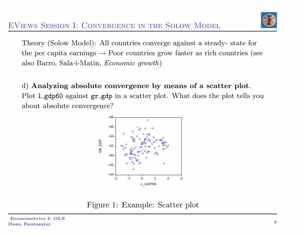
Theory (Solow Model): All countries converge against a steady- state for

the per capita earnings → Poor countries grow faster as rich countries (see

also Barro, Sala-i-Matin, Economic growth)

d) Analyzing absolute convergence by means of a scatter plot.

Plot l gdp60 against gr gdp in a scatter plot. What does the plot tells you

about absolute convergence?

-.04

-.02

.00

.02

.04

.06

.08

-2 -1 0 1 2 3

L_GDP60

GR

_GD

P

Figure 1: Example: Scatter plot

Econometrics I: OLS

Dean Fantazzini7


e) Analyzing absolute convergence by means of a regression.

Regress gr gdp on l gdp60 and a constant (click on gr gdp - press

STRG and click on l gdp60 - click on one of the series - OPEN

EQUATION - OK). Using the online help become acquainted with the

regression output (HELP - SEARCH - regression output). What does the

regression output tells you about absolute convergence?

LS GR GDP c L GDP60

Econometrics I: OLS

Dean Fantazzini8


f) Conditional convergence *. Regress gr gdp on l gdp60, gr pop, inv,

geetot and a constant. Interpret the regression output.

g) Setting the sample*. One of the important concepts in EViews is the

sample of observations. The sample is the set of observations to be

included in the analysis. Set the sample to OECD countries.

• SAMPLE - type in if-box: oecd=1.

• smpl if OECD=1

Econometrics I: OLS

Dean Fantazzini9


h) Redoing the analysis for OECD countries.

Repeat d), e) and f) with the new sample.

What changes? Interpret your results.

Econometrics I: OLS

Dean Fantazzini10

EViews Session II: Estimating a money demand equation

Some Premises...

Detection of Heteroscedasticity :

• Residual Plot;

• White Test;

• Breusch - Pagan test;

Detection of Autocorrelation:

• Residual Plot;

• Durbin-Watson test (... remember that X have to be deterministic);

d=2 → no autoc., d<2 → positive autoc., d>2 → negative

autocor.

• Breusch - Godfrey test

1. OLS to get the residuals et

2. et = γ1et−1 + . . . + γpet−p + x′

tβ + δt

3. H0 = n · R2∼ χ2

p

Econometrics I: OLS

Dean Fantazzini11


What to do in case of 1) Heteroscedasticity , 2) Autocorrelation?

• GLS (if Ω known), or FGLS

• OLS with 1) White VC matrix, or 2) Newey - West VC matrix

Empirical Example: Money demand.

• Transaction demand → GDP

• Speculation Demand → Bond rate, Money market rate

Econometrics I: OLS

Dean Fantazzini12


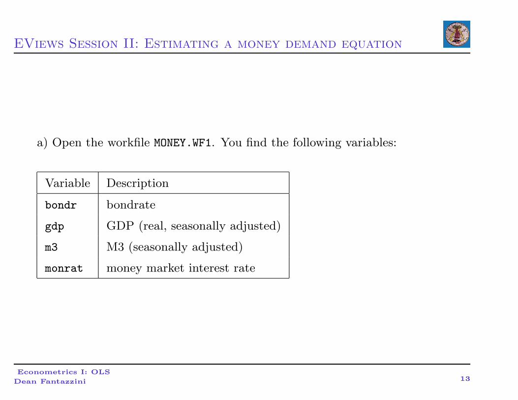
a) Open the workfile MONEY.WF1. You find the following variables:

Variable Description

bondr bondrate

gdp GDP (real, seasonally adjusted)

m3 M3 (seasonally adjusted)

monrat money market interest rate

Econometrics I: OLS

Dean Fantazzini13


b) Generate the following variables...

l_gdp = log(gdp), l_m3 = log(m3).

c) ... and estimate the following equation (you take into account the

transaction demand):

l_m3 = β0 + β1 · l_gdp + ε.

Save it as eq1.

d) Has β1 the sign you expected? Interpret.

Econometrics I: OLS

Dean Fantazzini14


e) Now you consider the speculation demand as well and estimate the

following equation:

l_m3 = β0 + β1 · l_gdp + β2 · monrat + β3 · bondr + ε.

Save it as eq2.

f) Have the coefficients the signs you expected? How do you interpret β1,

β2 and β3?

g) Now look at the residual plot. (View -> Actual, Fitted, Residual

-> Residual Graph). Do you find evidence of the presence of

heteroscedasticity and/or autocorrelation?

Econometrics I: OLS

Dean Fantazzini15


h) Consider the Durbin-Watson statistic:

1. Is there evidence of autocorrelation? If yes, positive or negative

correlation?

2. Which assumptions does an application of the Durbin-Watson test

require?

3. Are these assumptions valid in this case?

i) Run a Breusch-Godfreyserial correlation test including 4 lags.

1. What is the null hypothesis?

2. Procedure in EViews: View -> Residual Tests

-> Serial Correlation LM Test - 4.

3. Do you reject the null hypothesis on a 5% significance level?

Econometrics I: OLS

Dean Fantazzini16


j) Estimate the second equation, now using the Newey-West-VC-Matrix

(click on Options -> Heteroscedasticity -> Newey-West in the

specification window). Save the result as eq3. How do the t-values change

compared to equation 2?

k) Based on equation 3, test the following hypothesis on a 5% significance

level: i) β2 = 0, ii) β1 = 2 and iii) β3 < 0. Address the following points:

1. What are the null and the alternative hypothesis?

2. Calculate an appropriate test statistic.

3. Find the 5% critical value.

4. Do you reject the null hypothesis?

Econometrics I: OLS

Dean Fantazzini17


l) Test if the additional parameters in equation 2 (and equation 3) are

jointly significant.

Calculate the appropriate F statistic using two different ways:

1. Use the F test that is implemented in EViews.

2. Calculate the F test by hand using both regression outputs.

Econometrics I: OLS

Dean Fantazzini18

EViews Session III: Monte Carlo Simulation

A typical Monte Carlo simulation exercise consists of the following steps:

1. Specify the “true” model (data generating process) underlying the

data.

2. Simulate a draw from the data and estimate the model using the

simulated data.

3. Repeat step 2 many times, each time storing the results of interest.

4. The end result is a series of estimation results, one for each repetition

of step 2. We can then characterize the empirical distribution of these

results by tabulating the sample moments or by plotting the

histogram or kernel density estimate.

Econometrics I: OLS

Dean Fantazzini19


• Step 2 typically involves simulating a random draw from a specified

distribution. → EViews provides built-in pseudo-random number

generating functions for a wide range of commonly used distributions;

• The step that requires a little thinking is how to store the results from

each repetition (step 3). There are two methods that you can use in

EViews:

1. Storing results in a series;

2. Storing results in a matrix.

Econometrics I: OLS

Dean Fantazzini20


1) Storing results in a series (or group of series): The difficulty with

this approach is that series elements are most easily indexed by a sample in

EViews. To store the result from each replication as a different observation

in a series, you must shift the sample every time you store a new result.

Moreover, the length of the series will be constrained by the size of your

workfile sample: for example, if you wish to perform 1000 replications on a

workfile with 100 observations, you will not be able to store all 1000 results

in a series since the latter only has 100 observations.

Econometrics I: OLS

Dean Fantazzini21


2) Storing results in a matrix (or vector):

The matrix is indexed by its row-column position and its size is

independent of the workfile sample. For example, you can declare a matrix

with 1000 rows and 10 columns in a workfile with only 1 observation.

→ The disadvantage of the matrix method is that the matrix object does

not have as much built-in functions as a series object. For example, there

is no kernel density estimate view out of a matrix (which is available for a

series object).

For didactic purposes, I will illustrate both approaches. (My own

recommendation is a mixed approach. Store all the results in a matrix. If

you need to do further processing, convert the matrix into a group of

series.)

Econometrics I: OLS

Dean Fantazzini22


As a concrete example, consider the following exercise (3.26) from

Damodar Gujarati Basic Econometrics, 3rd edition:

Refer to the 10 X values of Table 3.2 (which are: 80, 100, 120, 140, 160,

180, 200, 220, 240, 260). Let Beta(1) = 2.5 and Beta(2) = 0.5. Assume

that the errors are distributed N(0, 9), that is, the errors are normally

distributed with mean 0 and variance 9. Generate 100 samples using these

values, obtaining 100 estimates of Beta(1) and Beta(2). Graph these

estimates. What conclusions can you draw from the Monte Carlo study?

Econometrics I: OLS

Dean Fantazzini23


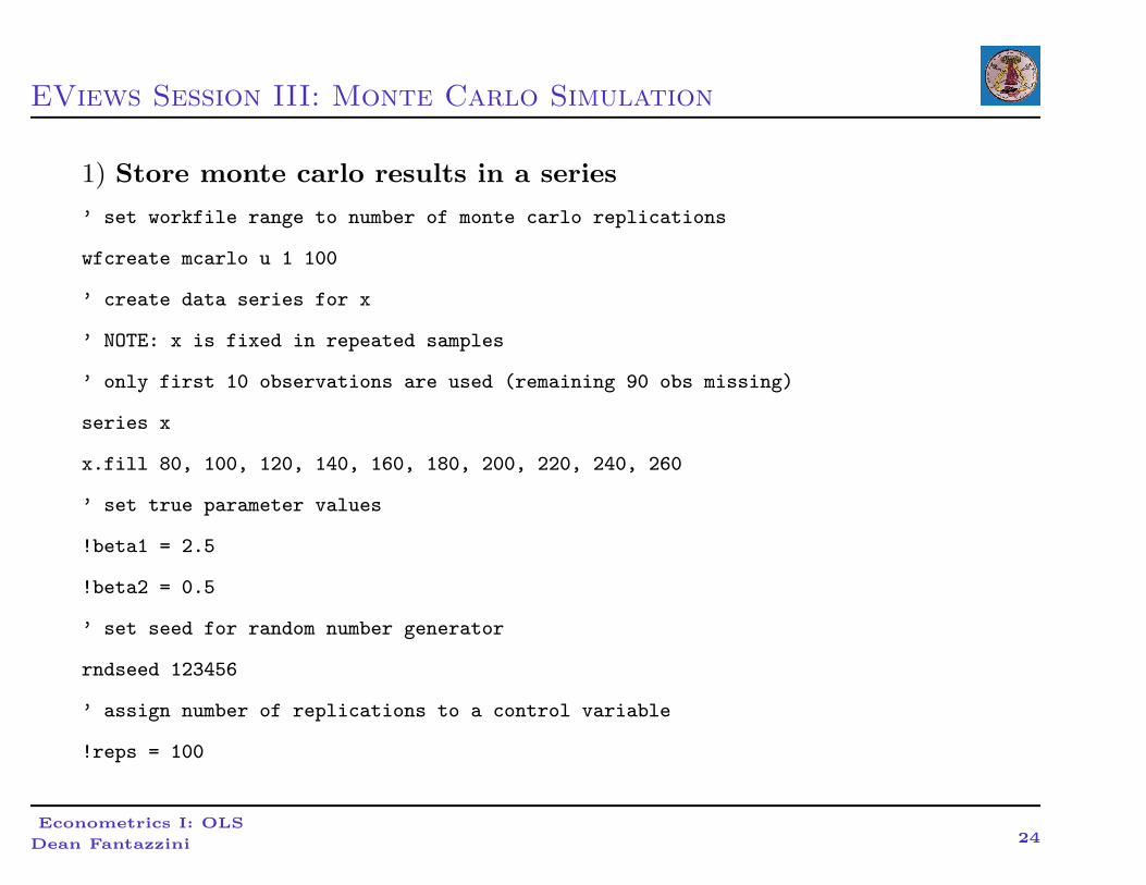
1) Store monte carlo results in a series

’ set workfile range to number of monte carlo replications

wfcreate mcarlo u 1 100

’ create data series for x

’ NOTE: x is fixed in repeated samples

’ only first 10 observations are used (remaining 90 obs missing)

series x

x.fill 80, 100, 120, 140, 160, 180, 200, 220, 240, 260

’ set true parameter values

!beta1 = 2.5

!beta2 = 0.5

’ set seed for random number generator

rndseed 123456

’ assign number of replications to a control variable

!reps = 100

Econometrics I: OLS

Dean Fantazzini24


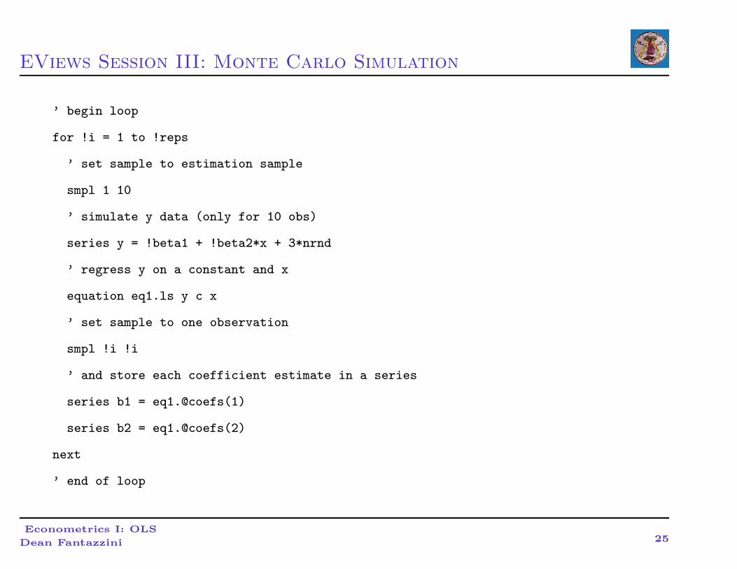
’ begin loop

for !i = 1 to !reps

’ set sample to estimation sample

smpl 1 10

’ simulate y data (only for 10 obs)

series y = !beta1 + !beta2*x + 3*nrnd

’ regress y on a constant and x

equation eq1.ls y c x

’ set sample to one observation

smpl !i !i

’ and store each coefficient estimate in a series

series b1 = eq1.@coefs(1)

series b2 = eq1.@coefs(2)

next

’ end of loop

Econometrics I: OLS

Dean Fantazzini25


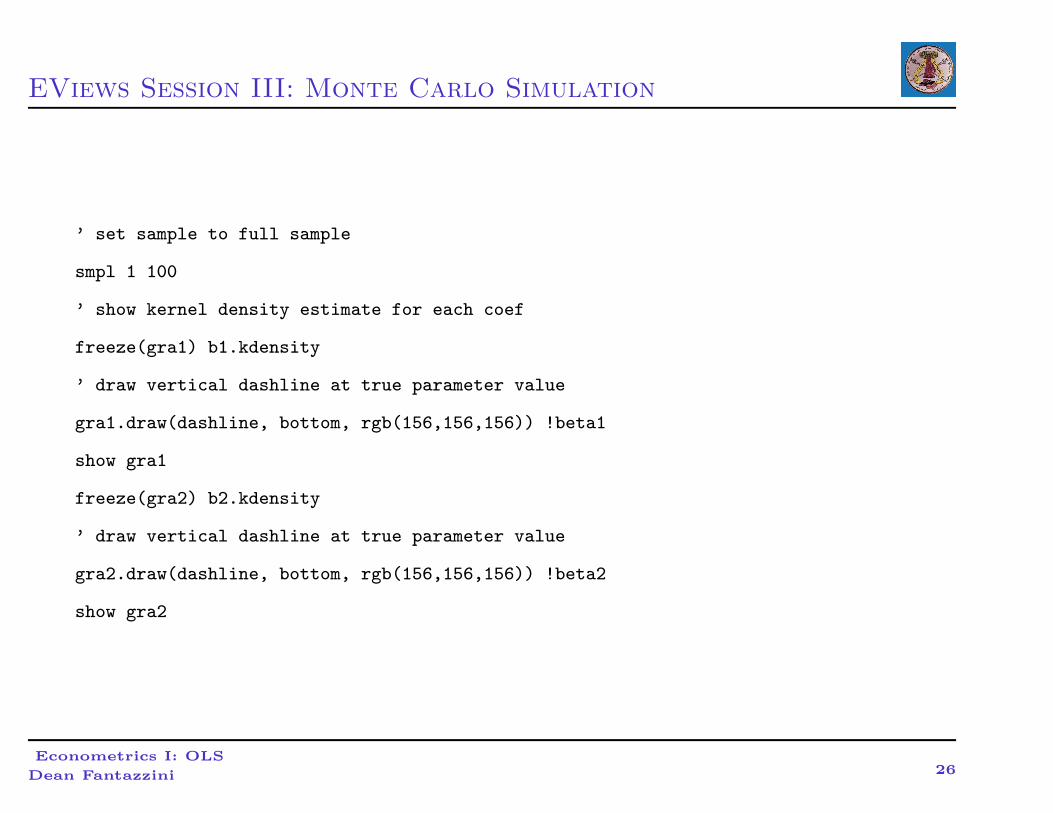
’ set sample to full sample

smpl 1 100

’ show kernel density estimate for each coef

freeze(gra1) b1.kdensity

’ draw vertical dashline at true parameter value

gra1.draw(dashline, bottom, rgb(156,156,156)) !beta1

show gra1

freeze(gra2) b2.kdensity

’ draw vertical dashline at true parameter value

gra2.draw(dashline, bottom, rgb(156,156,156)) !beta2

show gra2

Econometrics I: OLS

Dean Fantazzini26


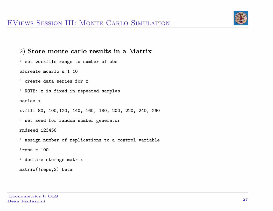
2) Store monte carlo results in a Matrix

’ set workfile range to number of obs

wfcreate mcarlo u 1 10

’ create data series for x

’ NOTE: x is fixed in repeated samples

series x

x.fill 80, 100,120, 140, 160, 180, 200, 220, 240, 260

’ set seed for random number generator

rndseed 123456

’ assign number of replications to a control variable

!reps = 100

’ declare storage matrix

matrix(!reps,2) beta

Econometrics I: OLS

Dean Fantazzini27


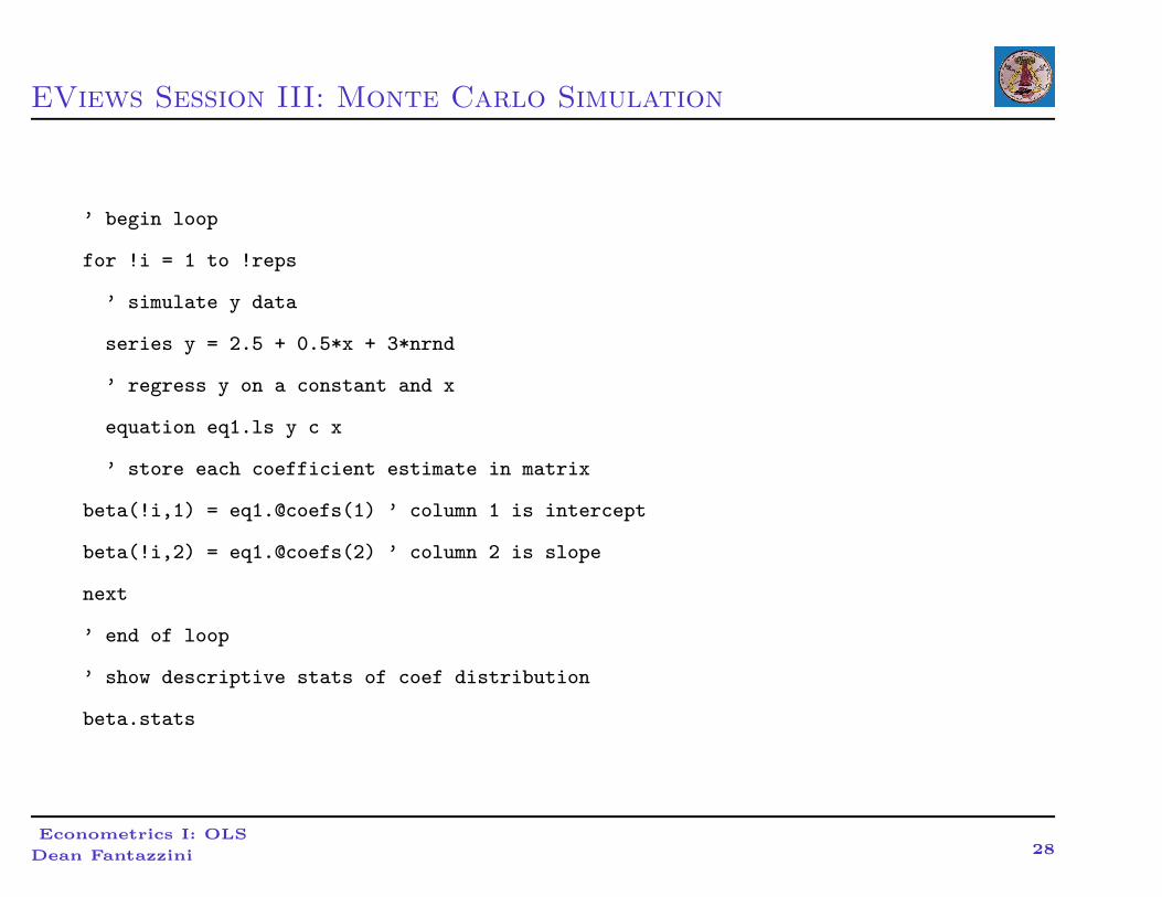
’ begin loop

for !i = 1 to !reps

’ simulate y data

series y = 2.5 + 0.5*x + 3*nrnd

’ regress y on a constant and x

equation eq1.ls y c x

’ store each coefficient estimate in matrix

beta(!i,1) = eq1.@coefs(1) ’ column 1 is intercept

beta(!i,2) = eq1.@coefs(2) ’ column 2 is slope

next

’ end of loop

’ show descriptive stats of coef distribution

beta.stats

Econometrics I: OLS

Dean Fantazzini28

econometrics i: ols

Documents