econometrics theory - geocities · econometrics theory ⁄ atsushi matsumoto y first draft:...
TRANSCRIPT
Econometrics Theory ∗
Atsushi MATSUMOTO †
First draft: 2007.10.201st Revied: 2008.1.28
2nd Revised: 2008.4.15
Abstract
This is the lecture note of introductory econometrics theory especially for graduate school studentsmajoring in economics. You should be familiar with basic linear algebra and calculus for fully under-standing the contents. Although this lecture note is based on the following references, all remainigerrors are mine.
References
Davidson, Russell and MacKinnon, James G.(2004) “Econometric theory and methods”,Oxford University Press
Davidson, Russell and MacKinnon, James G.(1993) “Estimation and inference in econometrics”,Oxford University Press
Greene, William H.(2003) “Econonmetric Analysis”, Prentice Hall
Wooldridge, Jeffrey M.(2006) “Introductory econometrics”, Thomson/South-Western
Wooldridge, Jeffrey M.(2002) “Econometric analysis of cross section and panel data”, MIT Press
∗You can use this lecture note freely only for your academic purposes. You must not distribute or modify it without mypermission. There must be some mistakes in proofs, calculations and English grammar. When you find them, please let meknow through an e-mail. But if you face serious problems with this lecture note, it is your responsibility.
†E-mail: [email protected]
1
Contents
1 Linear Regression Model 41.1 Introduction . . . . . . . . . . . . . . . . . . . . . . . . . . . . . . . . . . . . . . . . . . . . . 41.2 Estimation of simple regression model . . . . . . . . . . . . . . . . . . . . . . . . . . . . . . 41.3 Ordinaly Least Square Estimator . . . . . . . . . . . . . . . . . . . . . . . . . . . . . . . . . 5
2 Geometric Understanding of Linear Regression Model 52.1 Vector space . . . . . . . . . . . . . . . . . . . . . . . . . . . . . . . . . . . . . . . . . . . . . 52.2 Linear subspace and the geometry of the OLSE . . . . . . . . . . . . . . . . . . . . . . . . . 62.3 Orthogonal Projection . . . . . . . . . . . . . . . . . . . . . . . . . . . . . . . . . . . . . . . 7
3 The Frisch-Waugh-Lovell Theorem and Its Application 83.1 The concept of the FWL theorem . . . . . . . . . . . . . . . . . . . . . . . . . . . . . . . . . 83.2 The FWL theorem in detail . . . . . . . . . . . . . . . . . . . . . . . . . . . . . . . . . . . . 93.3 Goodness of fit . . . . . . . . . . . . . . . . . . . . . . . . . . . . . . . . . . . . . . . . . . . 11
4 The Properties of the OLSE 114.1 The unbiasedness of OLSE . . . . . . . . . . . . . . . . . . . . . . . . . . . . . . . . . . . . 114.2 The consistency of OLSE . . . . . . . . . . . . . . . . . . . . . . . . . . . . . . . . . . . . . 134.3 The variance-covariance matrix of the OLSE . . . . . . . . . . . . . . . . . . . . . . . . . . 134.4 Efficiency of the OLSE . . . . . . . . . . . . . . . . . . . . . . . . . . . . . . . . . . . . . . . 144.5 Residuals and error terms . . . . . . . . . . . . . . . . . . . . . . . . . . . . . . . . . . . . . 15
5 Missspecification 165.1 Overspecification of the linear regression model . . . . . . . . . . . . . . . . . . . . . . . . . 165.2 Underspecification of the linear regression model . . . . . . . . . . . . . . . . . . . . . . . . 17
6 Hypothesis Testing 186.1 Test of a single restriction . . . . . . . . . . . . . . . . . . . . . . . . . . . . . . . . . . . . . 206.2 Tests of several restrictions . . . . . . . . . . . . . . . . . . . . . . . . . . . . . . . . . . . . 22
7 Tests based on Simulation 237.1 Parametric/Non-parametric Bootstrap . . . . . . . . . . . . . . . . . . . . . . . . . . . . . . 237.2 Bootstrap test . . . . . . . . . . . . . . . . . . . . . . . . . . . . . . . . . . . . . . . . . . . . 24
8 Non Linear Model 248.1 The method of moments estimator and its property . . . . . . . . . . . . . . . . . . . . . . . 248.2 The concept of identification . . . . . . . . . . . . . . . . . . . . . . . . . . . . . . . . . . . 258.3 The consistency of the NLE . . . . . . . . . . . . . . . . . . . . . . . . . . . . . . . . . . . . 258.4 Asymptotic normality and asymptotic efficiency . . . . . . . . . . . . . . . . . . . . . . . . . 258.5 Non linear least square . . . . . . . . . . . . . . . . . . . . . . . . . . . . . . . . . . . . . . . 268.6 Newton’s method . . . . . . . . . . . . . . . . . . . . . . . . . . . . . . . . . . . . . . . . . . 278.7 The Gauss-Newton regression . . . . . . . . . . . . . . . . . . . . . . . . . . . . . . . . . . . 28
9 Generalized Least Squares 299.1 Basic idea of GLS . . . . . . . . . . . . . . . . . . . . . . . . . . . . . . . . . . . . . . . . . 299.2 Geometry of GLSE . . . . . . . . . . . . . . . . . . . . . . . . . . . . . . . . . . . . . . . . . 309.3 Interpretting GLSE . . . . . . . . . . . . . . . . . . . . . . . . . . . . . . . . . . . . . . . . . 319.4 Heteroskedasticity . . . . . . . . . . . . . . . . . . . . . . . . . . . . . . . . . . . . . . . . . 319.5 Serial correlation . . . . . . . . . . . . . . . . . . . . . . . . . . . . . . . . . . . . . . . . . . 33
10 Analysis of Panel Data 3410.1 Fixed effect model . . . . . . . . . . . . . . . . . . . . . . . . . . . . . . . . . . . . . . . . . 3510.2 Random effect model . . . . . . . . . . . . . . . . . . . . . . . . . . . . . . . . . . . . . . . . 35
2
11 Instrumental Variable Method 3711.1 IV estimator . . . . . . . . . . . . . . . . . . . . . . . . . . . . . . . . . . . . . . . . . . . . 3911.2 The number of IV and the identification . . . . . . . . . . . . . . . . . . . . . . . . . . . . . 3911.3 Testing based on IV . . . . . . . . . . . . . . . . . . . . . . . . . . . . . . . . . . . . . . . . 40
12 Maximum Likelihood 4212.1 The properties of MLE . . . . . . . . . . . . . . . . . . . . . . . . . . . . . . . . . . . . . . . 4212.2 Asymptotic tests based on likelihood . . . . . . . . . . . . . . . . . . . . . . . . . . . . . . . 4612.3 Model selection based on likelihood . . . . . . . . . . . . . . . . . . . . . . . . . . . . . . . . 47
13 Generalized Method of Moments 4813.1 GMM estimator for linear regression models . . . . . . . . . . . . . . . . . . . . . . . . . . . 4813.2 Efficient GMME and feasibe efficient GMME . . . . . . . . . . . . . . . . . . . . . . . . . . 4913.3 Tests based on GMM . . . . . . . . . . . . . . . . . . . . . . . . . . . . . . . . . . . . . . . . 5013.4 GMME for nonlinear models . . . . . . . . . . . . . . . . . . . . . . . . . . . . . . . . . . . 50
14 Limited Dependent Variables Models 5314.1 Binary response models . . . . . . . . . . . . . . . . . . . . . . . . . . . . . . . . . . . . . . 5314.2 Specification test . . . . . . . . . . . . . . . . . . . . . . . . . . . . . . . . . . . . . . . . . . 5414.3 Multinomial/Conditional choice model . . . . . . . . . . . . . . . . . . . . . . . . . . . . . . 55
15 Various Convergence and Useful Results 5715.1 Convergence in probability . . . . . . . . . . . . . . . . . . . . . . . . . . . . . . . . . . . . 5715.2 Convergence in mean square . . . . . . . . . . . . . . . . . . . . . . . . . . . . . . . . . . . . 5815.3 Convergence in distribution . . . . . . . . . . . . . . . . . . . . . . . . . . . . . . . . . . . . 5915.4 Law of large numbers for weakly stationary process . . . . . . . . . . . . . . . . . . . . . . . 63
3
1 Linear Regression Model
1.1 Introduction
Let us consider the simple linear regression model below. The word ”linear” means that the model is linearwith respect to parameters. The linearity implies that the marginal effect does not depend on the level ofregressors.
yt = β1 + β2xt + ut, for t = 1, · · · , n.
Here we call yt explained variable, or dependent variable, xt explanatory variable, or independent variable,β1, β2 parameters, and ut disturbance or error term. In addition to them, t denotes each observation andn is the total observations. By the point of view of estimation, (xt, yt)n
t=1 is observed set, while utnt=1
is un-observed set. β1 and β2 are unknown constant to be estimated, which represent the marginal andseparate effects of the regressors. For instance, β2 represents the change in the dependent variable whenthe second regressors xt increses by one unit while other regressors are fixed to be constant. This meansthat ∂yt/∂xt = β2.
As to the disturbances utnt=1, we assume that E(ut) = 0 and sometimes assume more. This assumption
is valid because of the reason that individuals in economics theory can be seen as economic men, or averagemen. In economic theory, we regard them as rational so if their characters are varying, consequentlyE(ut) = 0, that is, the sum of their characters is trivial.
Then we need to estimate unknown parameters β1 and β2 based on the observed set (xt, yt)nt=1 and
the assumption that E(ut) = 0. For the model yt = β1 + β2xt + ut, we take expectaion but xt is randomvariable so that we take conditional expectaion given xt. Hence we obtain:
E(yt | xt) = E(β1 + β2xt + ut | xt)= β1 + β2E(xt | xt) + E(ut | xt)= β1 + β2xt + E(ut | xt).
Assuming that E(ut | xt) = 0, we get E(yt | xt) = β1 + β2xt. Note that E(ut | xt) = 0 implies E(ut) = 0but not vice versa. Since Ex
(Eu(ut | xt)
)= Eu(ut), if E(ut | xt) = 0 then we have E(ut) = 0. This logic is
valid because of the proof below:
Eu(ut) =∫
utf(ut)dut
=∫
ut
∫f(xt, ut)dxtdut
=∫ ∫
utf(ut | xt)dutf(xt)dxt =∫
Eu(ut | xt)f(xt)dxt = Ex
(Eu(ut | xt)
),
where f(·) is the PDF and f(·|·) is the conditional PDF. If we assume that E(ut | xt) = 0, then we haveE(ut) = and E(xtut) = 0, which can be obtained from:
E(xtut) = Ex
(E(xtut | xt)
)= Ex
(xtE(ut | xt)
)= 0.
This logic can be applied to vector notation that E(u|X) = 0 implies E(u) = 0 and E(X ′u) = 0. This isbecause E(X ′u) = EX
(E(X ′u|X)
)= EX
(X ′E(u|X)
)= 0.
1.2 Estimation of simple regression model
For the model yt = β1 + β2xt + ut, we assume that E(ut | xt) = 0. Then we have E(utxt) = 0 andE(ut) = 0. The Method of Moment uses these assumptions. By using these assumptions, we get:
E(utxt) = E(xt(yt − β1 − β2xt)) = 0
=⇒ n−1n∑
t=1
xtut = n−1n∑
t=1
xt(yt − β1 − β2xt) = 0 ∴n∑
t=1
xtyt − β1
n∑t=1
xt − β2
n∑t=1
x2t = 0,
E(ut) = E(yt − β1 − β2xt) = 0
=⇒ n−1n∑
t=1
ut = n−1n∑
t=1
(yt − β1 − β2xt) = 0 ∴n∑
t=1
yt − β1
n∑t=1
−β2
n∑t=1
xt = 0.
4
Hence we can calculate β1 and β2 which satisfy the equations above. For the simple regression modelyt = β1 + β2xt + ut, letting xt = (1, xt) and β = (β1, β2), we can rewrite this model as:
yt = x′tβ + ut, for t = 1, · · · , n.
Collecting all t = 1, · · · , n and letting y = (y1 · · · yn)′, X = (x1 · · ·xn)′ and u = (u1 · · ·un)′, we have:
y = Xβ + u.
And, as before, the assumption as to the disturbance also can be written as in the vector form E(X ′u) = 0.The orthogonal condition E(X ′u) = 0 takes the expectaion. For estimation, however, we use arithmeticmean of X ′u instead of its expectaion. By this logic, we have n−1X ′u = 0, equivalently, X ′u = 0, hencewe obtain:
X ′(y −X ′β) = 0 ⇔ X ′y = X ′Xβ ∴ β = (X ′X)−1X ′y,
where this calculation is valid only if X ′X is full rank so that the inverse matrix of X ′X exists.
1.3 Ordinaly Least Square Estimator
Let us consider the regression model y = Xβ + u. To obtain the OLSE, letting S(β) be the suared normof u = y − Xβ, we solve the minimization problem which takes the form of:
β = arg minS(β) = (y −Xβ)′(y −Xβ)= y′y − y′Xβ − β′X ′y + β′X ′Xβ
= y′y − 2y′Xβ + β′X ′Xβ.
In order to obatin OLSE β, we differentiate S(β) with respecto β and set ∂S(β)/∂β = 0:
∂S(β)∂β
= −2X ′y + 2X ′Xβ = 0.
The following formulas give the idea of differentiation of matrix: ∂(y′Xβ)/∂β = (y′X)′ and ∂(β′X ′Xβ)/∂β =2(X ′X)β since X ′X is symmetric. Hence we obatain β = (X ′X)−1X ′y. Notice that the FOCs guaranteethe existence of the minimum, which can be confirmed by the fact that the second derivative
∂2S(β)∂β∂β′
= X ′X.
is positive semidefinite, which means that there exists the minumum of S. Note that the assertion above isvalid only if X ′X is full rank, which means that the rank of X is k and there exists no multicollinearity.
2 Geometric Understanding of Linear Regression Model
2.1 Vector space
Consider any n-dimensional vector x = (x1 · · ·xn)′ and y = (y1 · · · yn)′ with x,y ∈ <n. Firstly the length,or norm, of a vector x is defined by:
‖x‖ :=(x′x
)1/2 =( n∑
i=1
x2i
)1/2
.
Then the inner product of x and y can be defined:
〈x,y〉 := x′y = ‖x‖‖y‖ cos θ, (0 ≤ θ ≤ π),
where θ is an angle between x and y. The space(subset of <n) in which distance and inner product aredefined is called Euclidian space and is denoted by En. Of course, En ⊂ <n.
Rewriting the above definition of inner product, we have:
cos θ =x′y
‖x‖‖y‖ ,
5
which is the correlation coefficient(ρ) of x and y. Since the function cos θ is monotonically decreasing in0 ≤ θ ≤ π, we easliy see that −1 ≤ ρ = cos θ ≤ 1. This is the reason why any correlation coefficientsare between −1 and 1 and why the positive(negative) value of ρ indicates the positive(negative) relationbetween variables. Now by the definition of inner product, we have 〈x,y〉 = x′y so that
〈x,y〉 = x′y = ‖x‖‖y‖ cos θ,
thus we get Caushy-Schwartz inequality:
| x′y |=| ‖x‖‖y‖ cos θ |= ‖x‖‖y‖ cos θ ≤ ‖x‖ ‖ y‖.
A basis of a vector space is an important concept. The basis of a vector space Vn is a set of vectorsin Vn and is defined to satisfy (1) each basis is linearly independent 1) and (2)any vector in Vn can berepresented as a linear combination of the bases. Given a space, the choices of bases are infinite. But,the cardinal number which consist of basis is independent of such choices. The basis in Vn consists of nvectors. Therefore we see that the dimension of a vector space is equal to the cardinal number.
2.2 Linear subspace and the geometry of the OLSE
We consider the linear regression model with the form y = Xβ + u, where y and u are n-dimensional,β is k-dimensional, and X is n × k. The regressand y and the regressor X can be thought of as vectorsin En so that we can represent their relationship geometically. But to go on, we need to understand theconcept of a subset of a Euclidian space En.
Let X = (x1 · · ·xk) with xj = (x1j · · ·xnj)′ for j = 1, · · · , k. Each xj can be thought of as a basisvector. Then the subspace associated with these k basis vectors is denoted by ℘(X), or ℘(x1, · · · ,xk),and is defined as:
℘(x1, · · · ,xk) :=
z ∈ En∣∣z =
k∑
j=1
bjxj , bj ∈ <
,
which is the subspace formed as a linear combination of the x’s. On the other hand, the orthogonalcomplement of ℘(X), denoted by ℘⊥(X), is defined by:
℘⊥(x1, · · · ,xk) :=
w ∈ En∣∣w′z = 0 for all z ∈ ℘(X)
.
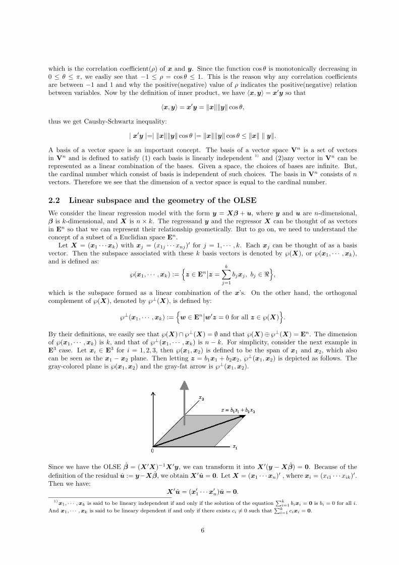
By their definitions, we easily see that ℘(X)∩℘⊥(X) = ∅ and that ℘(X)⊕℘⊥(X) = En. The dimensionof ℘(x1, · · · ,xk) is k, and that of ℘⊥(x1, · · · ,xk) is n − k. For simplicity, consider the next example inE3 case. Let xi ∈ E3 for i = 1, 2, 3, then ℘(x1,x2) is defined to be the span of x1 and x2, which alsocan be seen as the x1 − x2 plane. Then letting z = b1x1 + b2x2, ℘⊥(x1,x2) is depicted as follows. Thegray-colored plane is ℘(x1,x2) and the gray-fat arrow is ℘⊥(x1,x2).
Since we have the OLSE β = (X ′X)−1X ′y, we can transform it into X ′(y −Xβ) = 0. Because of thedefinition of the residual u := y−Xβ, we obtain X ′u = 0. Let X = (x1 · · ·xn)′ , where xi = (xi1 · · ·xik)′.Then we have:
X ′u = (x′1 · · ·x′n)u = 0.
1)x1, · · · ,xk is said to be lineary independent if and only if the solution of the equation
Pki=1 bixi = 0 is bi = 0 for all i.
And x1, · · · ,xk is said to be lineary dependent if and only if there exists ci 6= 0 such thatPk
i=1 cixi = 0.
6
This result implies that x′iu = 0, that is, xi and u are orthogonal. This also means that the explanatoryvariables and the residuals are orthogonal. Consequently, since X = (x1 · · ·xk) , where xi = (x1i · · ·xni)′
and β = (β1 · · ·βk)′ and since 〈u,xi〉 = 0, we find:
y := Xβ =k∑
i=1
βixi =∈ ℘(X),
u := y − y ∈ ℘⊥(X).
2.3 Orthogonal Projection
A projectoin is a mapping that takes each point of En into a point in a subspace of En, while leavingall points in that subspace unchanged. We apply this notation to the OLS regression. If y = z + w fory ∈ En, where z ∈ ℘(X), w ∈ ℘⊥(X), then z is called the orthogonal projection of y. Let z = PXy, w =(I − PX)y. PX is called projection matrix which takes the form of:
PX = X(X ′X)−1X ′.
Based on the concept of the OLSE, we have y = y + u with y ∈ ℘(X) and u ∈ ℘⊥(X) so that it is naturalto let z = y and w = u. The OLS regression can be viewed as the mapping of y into two spaces ℘(X)and ℘⊥(X). Hence we get:
z = y = Xβ
= (X(X ′X)−1X ′)y := PXy.
Similarly we obtain:
w = u = y − y
= y − PXy
= (I −X(X ′X)−1X ′))y := MXy.
Therefore, because y ∈ ℘(X) and u ∈ ℘⊥(X), we get PXy ∈ ℘(X) and MXy ∈ ℘⊥(X). Here noticethat
PX y = y,
MX u = u.
We have learned that PX is the operator to project onto ℘(X). But y has been already onto ℘(X). Thusy is not influenced by PX . And MX is the operator to project onto ℘⊥(X). But u hsa been already onto℘⊥(X). Therefore u is not influenced by MX .
The following properties of projection matrix are useful. Firstly, PX and MX are idempotent since
PXPX = X(X ′X)−1X ′ ·X(X ′X)−1X ′
= X(X ′X)−1X ′ = PX
MXMX = (I − PX)(I − PX),
= I2 − PX − PX + P 2X = I − PX = MX .
This property holds for any projection matrix and this logic is the same as that of PX y = y and MX u = u.By the first PX(or MX) in the equation above, we can project any vector onto ℘(X)(or ℘⊥(X)) so thatif we operate PX(or MX) again, we cannot project more. Next PX and MX are orthogonal since
PXMX = PX(I − PX) = O.
This property is called annihilation, that is, PX and MX annihalete each other. This logic is easy to beunderstood. Since PX projects onto ℘(X) and MX projects onto ℘⊥(X), the only point that belongs toboth ℘ and ℘⊥ is zero. Also the property that PX + MX = I and that PX and MX are symmetric canbe confirmed immediately. Note that for a nonsingular k × k matrix A, the subspace of XA satisfies:
℘(X) = ℘(XA).
7
This result is valid because of the calculation below:
PXA = XA(A′X ′XA)−1A′X
= XAA−1(X ′X)−1(A′)−1A′X ′ = X(X ′X)−1X ′ = PX ,
or letting X = (x1 · · ·xk), A = (a1 · · ·ak)′ then we have:
XA = x1a1 + · · ·+ xkak,
which is the linear combination of xi so that XA ∈ ℘(X) is clear.
3 The Frisch-Waugh-Lovell Theorem and Its Application
3.1 The concept of the FWL theorem
Consider the following simple regression model for simpliciy:
y = ıβ1 + xβ2 + u,
where y = (y1 · · · yn)′, ı is an n-dimensional vector such as ı = (1 · · · 1)′, x = (x1 · · ·xn)′ and u =(u1 · · ·un)′. And let us define z = (z1 · · · zn)′, where zi = xi − x. Then we can transform the modely = ıβ1 + xβ2 + u, by the definition of z, into:
y = ıβ1 + (z + ıx)β2 + u
= ıβ1 + ıxβ2 + zβ2 + u
= ı(β1 + xβ2) + zβ2 + u.
Here note that the inner product of ı and z, or 〈ı,z〉, is 0, that ı′Mı = 0′ by the property of the orthogonalprojection matrix, and that, using projection matrix, z can be represented as:
z = x− ıx = x− ı(ı′ı)−1ı′x
= (I − ı(ı′ı)−1ı′)x := Mıx.
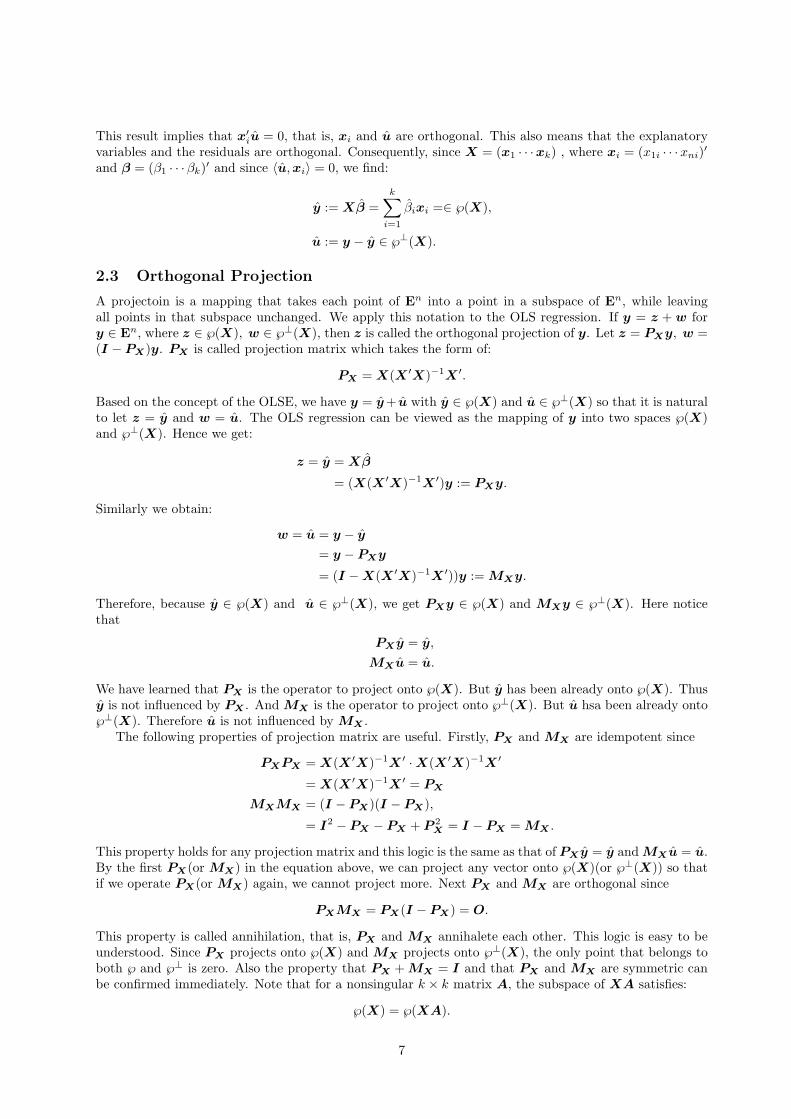
Consider the regression y on x and ı(left figure) and the regression y = ıα1 +zα2 +u(right figure), whereα = β1 + xβ2 and α2 = β2.
The gray-fat arrow, which takes the vector form of xβ2 − zα2, can be seen as the projection of xβ2 ontoı. Therefore it must hold that
zα2 − xβ2 = (ı(ı′ı)−1ı′)xβ2.
This can be transformed into:
zα2 = xβ2 − (ı(ı′ı)−1ı′)xβ2 = β2(I − ı(ı′ı)−1ı′)x.
The part (I − ı(ı′ı)−1ı′)x can be seen as the residual of the regression of x on ı. Here z and ı areorthogonal to one another. This is the advantage when explanatory variables are orthogonal. In this case,although explanatory variables x and 1 are not orthogonal, explanatory variables z and 1 are orthogonal.But both regression( y = 1β1 + xβ2 + u and y = 1α1 + zα2 + u) return the same OLSE, α2 = β2. The
8
advantage of orthogonality between explanatory variables are understood in matrix algebra. The detail isargued in the next sub section.
Next consider obtaining β2 in the models below:
y = ıβ1 + xβ2 + u,
y = ıα1 + zβ2 + u, where z = x− ıx,
y = zβ2 + v.
The problem here is that although all β2 is the same, their residuals are different.
3.2 The FWL theorem in detail
Let us consider the partitioned regression taking the form of:
y = X1β1 + X2β2 + u,
where X = (X1 X2) with X1 being n×k1 and X2 being n×k2 matrix with k = k1 +k2, and β′ = (β′1 β′2)with β1 being k1-dimensional and β2 being k2-dimensional vector. Our interest is the regression coefficientsβ1 and β1 which minimize the sum of squared residuals S(β1,β2):
S(β1,β2) = (y −X1β1 + X2β2)′(y −X1β1 + X2β2)= y′y − y′X1β1 − y′X2β2 − β′1X
′1y + β′1X
′1X1β1 + β′1X
′1X2β2 − β′2X
′2y + β′2X
′2X1β1 + β2X
′2X2β2
= y′y − 2y′X ′1β1 − 2y′X2β2 + 2β′1X
′1X2β2 + β′1X
′1X1β1 + β′2X
′2X2β2.
To obtain the FOCs to minimize, we differentiate S(β1,β2) with respect to β1 and β2 and get:
∂S(β1,β2)∂β1
= (−2y′X1)′ + (2X ′1X1)β1 + 2X ′
1X2β2 = 0,
∂S(β1,β2)∂β2
= (−2y′X2)′ + (2X ′2X2)β2 + 2X ′
2X1β1 = 0.
Thus the nomal equation is given by:(
X ′1X1 X ′
1X2
X ′2X1 X ′
2X2
)(β1
β2
)=
(X ′
1yX ′
2y
).
And solving the equations above with respect to β1, we have:
X ′1X1β1 = X ′
1y −X ′1X2β2 ⇐⇒ β1 = (X ′
1X1)−1X ′1y − (X ′
1X1)−1X ′1X2β2,
= (X ′1X1)−1X ′
1y − (X ′1X1)−1X ′
1X2β2
= (X ′1X1)−1X ′
1(y −X2β2).
(1)
Supposing that X ′1X2 = O, that is, supposing that X1 and X2 are orthogonal to one another, we get
β1 = (X ′1X1)−1X ′
1y, which is just the coefficient vector in the regression of y on X1. We, therefore, havethe folloing theorem.
Theorem: Orthogonal Partitioned Regression In the multiple least square regression of y on X1 andX2, that is, the regression y = X1β1 + X2β2 + u, if the two sets of variables X1 and X2 are orthogonal,then the separate coefficient vectors can be obtained from separate regressions of y on X1 alone and y onX2 alone. Therefore, if X1 and X2 are orthogonal,
β1 = (X ′1X1)−1X ′
1y, β2 = (X ′2X2)−1X ′
2y.
Next consider the case in which X1 and X2 are not orthogonal. By the 2nd equation of the noramlequation, we have:
X ′2X1β1 + X ′
2X2β2 = X ′2y. (2)
9
Then inserting Eq.(1) into Eq(2), we obtain:
X ′2X1
((X ′
1X1)−1X ′1(y −X2β2)
)+ X ′
2X2β2 = X ′2y
∴ X ′2X1(X ′
1X1)−1X ′1y −X ′
2X1(X ′1X1)−1X ′
1X2β2 + X ′2X2β2 = X ′
2y(X ′
2X2 −X ′2X1(X ′
1X1)−1X ′1X2
)β2 = X ′
2y −X ′2X1(X ′
1X1)−1X ′1y
X ′2
(I −X1(X ′
1X1)−1X ′1
)X2β2 = X ′
2y −X ′2X1(X ′
1X1)−1X ′1y.
Thus we get:
β2 =(X ′
2(I −X1(X ′1X1)−1X ′
1)X2
)−1(X ′
2y −X ′2X1(X ′
1X1)−1X ′1y
)
=(X ′
2(I −X1(X ′1X1)−1X ′
1)X2
)−1(X ′
2(I −X ′1(X
′1X1)−1X ′
1)y)
= (X ′2M1X2)−1(X ′
2M1y),
where M1 := I − X1(X ′1X1)−1X ′
1. This matrix is the residual maker such that (1)M1X2 is the theresidual of the regression X2 on X1, and (2)M1y is the residual of the regression y on X1. Then let usconsider M1X2, which represents the residual vector of the regression of X2 on X1 and which satisfies:
β2 = (X ′2M1X2)−1(X ′
2M1y)
= (u′2u2)−1(u′2u1),
where u1 := M1y, which is the residual of the regression of y on X1, and u2 := M1X2, which is theresidual of the regression of X2 on X1. Hence we have the following theorem.
Theorem: Frisch-Waugh-Lovell In the linear regression of y on X1 and X2, the β2 is the set ofcoefficients in the regression of u1 against u2, which are the residual of the regression y against X1 andof the regression X2 against X1 respectively. That is, β2 is the coefficient of the model:
u1 = u2β2 + ε, or equivalently M1y = M1X2β2 + ε.
Proof: Let us consider the two models, which are given by:
y = X1β1 + X2β2 + u,
M1y = M1X2β2 + M1u.
But each model can be rewritten as:
y = X1β1 + X1β2 + MXy, (3)
M1y = M1X2β2 + ε. (4)
Now for Eq.(3), premultiplying both sides by X ′2M1 we obtain:
X ′2M1y = X ′
2M1X1β1 + X ′2M1X2β2 + X ′
2M1MXy
= X ′2M1X2β2,
(5)
where the last equality holds from that M1X1 = O and that X ′2M1MX = O
2) . Consequently weobtain β2 = (X ′
2M1X2)−1X ′1M1y from Eq.(5) under the condition that X ′
2M1X2 is full rank. And as toEq.(4), the simple formula gives β2 = (X ′
2M1X2)−1X ′1M1y. Therefore β2 in Eq.(3) and that in Eq.(5)
2)Note that PXP1 = P1. Then we have:
MXM1 = (I − PX)(I − P1) = I − PX = MX .
Hence, we have (MXM1X2)′ = (MXX2)′ = O.
10
are identical. Next consider the residuals of the two models. For Eq.(3), premultiplying both sides by M1
we have:
M1y = M1X2β2 + M1MXy
= M1X2β2 + MXy.
Comparing this result with the Eq.(4), we find that MXy = ε, which means that the residual of Eq.(3)and that of Eq.(4) are identical. Hence we completed all the proof.¥
3.3 Goodness of fit
One indicator of goodness of fit is the coefficient of determination denoted as R2. This indicator uses theTSS decomposition: TSS=ESS+RSS. Applying Pythagoras’ Theorem, we get:
‖y‖2 = ‖Xβ‖2 + ‖u‖2,∴ y′y︸︷︷︸
TSS
= β′X ′Xβ + u′u = β′X ′Xβ︸ ︷︷ ︸ESS
+(y −Xβ)′(y −Xβ)︸ ︷︷ ︸RSS
.
Then R2 is defined by:
R2 := 1− RSSTSS
= 1− ‖u‖2‖y‖2 ,
which indicates that, the less the RSS becomes, the large R2 becomes. We easily find that R2 is between0 and 1. If RSS is equal to 0 then R2 = 1, while R2 = 0 if the estimated model does not explain y atall. But this R2 does not require the deviation from the mean. The R2 which uses the deviation from themean is called centered R2. It is defined by:
R2c :=
‖PXM1y‖2‖M1y‖2 or R2
c =‖y − ıy‖2‖y − ıy‖2 =
‖Mıy‖2‖Mıy‖2 , where Mı = I − ı(ı′ı)−1ı′.
A linear algebra calculation enables us to rewrite the expression above as:
R2c =
‖Mıy‖2‖Mıy‖2 =
y′Mıy
y′Mıy
=y(I − ı(ı′ı)−1ı′)yy(I − ı(ı′ı)−1ı′)y
=y′y − ny2
y′y − ny2,
where the last equality holds from the fact that ¯y = y. Note that if the regressors do not include a constantterm then centered R2 can be negative.
4 The Properties of the OLSE
4.1 The unbiasedness of OLSE
The one of the indicator of goodness of the OLSE is unbiasedness. If θn is an estimator of θ based onsample size n and if it satisfies:
E(θn) = θ, for all n,
then θn is unbiased estimator of θ. Another definition is, by defining the bias of θn to be E(θn)− θ, andif the bias is equal to zero, then the estimator θn is said to be unbiased estimator of θ. Then consider thecase of the OLSE β, which is given by β = (X ′X)−1X ′y. Now suppose that the Data Genarating Processis y = Xβ + u so that the problem like misspecification does not occur. The conditional expectation of βgiven X is
E(β | X) = E((X ′X)−1X ′y | X)
= E((X ′X)−1X ′Xβ + u | X)
= E((X ′X)−1X ′X | X) + E((X ′X)−1X ′u | X)
= β + (X ′X)−1E(u | X) = β.
11
The last equality holds from the assumption that E(u | X) = 0, which means that the explanatoryvariables X are uncorrelated with the disturbance u. This also means that the explanatory variables of Xis exogenous. An exogenous variable has its origins out side the model, while the mechanism generatingan endogenous variable is inside the model. It is obvious that
E(β | X) = E(β) = β.
The equation above implies that β is unbiased estimator of β. The cases in which the unbiasdness of theOLSE is not met are, for example, that there are lagged dependent variable in explanatory varibale, thatis, explanatory variable contains lagged explained varibale like yt = αyt−1 + εt. In this case, yt is said tofollow AR(1). Now consider the unbiasdness of α in AR(1) model. The OLSE of this model is given by:
α =∑n
t=1 ytyt−1∑nt=1 y2
t−1
, y0 given,
where εt ∼ i.i.d. N (0, σ2). Then, taking the expectaion, we get:
E(α) = E
(∑nt=1 ytyt−1∑nt=1 y2
t−1
)= E
(∑nt=1 yt−1(αyt + εt)∑n
t=1 y2t−1
)
= α + E
(∑nt=1 yt−1εt∑nt=1 y2
t−1
).
But it isn’t generally valid that E(εt | yt) = 0. Hence there exists bias E(∑n
t=1 yt−1εt/∑n
t=1 y2t−1) in AR(1)
model. In order for this logic to be more precisely, we consider another AR(1), which takes the vector formof:
y = β1ı + β2y1 + u, where u ∼ i.i.d.(0, σ2I).
In the model above, y has typical element yt, and y1 has typical element yt−1. Now notice that E(u |y1) 6= 0 because yt−1 depends on ut−1, ut−2, · · · . Applying the FWL theorem to the model, we have:
ε = β2ε1 + η,
where ε is the residual of the regression of y on ı, and ε1 is that of the regression of y1 on ı. Now theOLSE of β2 is obtained and, if we replace y with β1ı + β2y1 + u, it can be rewritten as:
β2 = (ε′1ε1)−1ε′1ε
= (y′1M1y1)−1(y′1M1y)
= (y′1Mıy1)−1(y′1Mı(β1ı + β2y1 + u))
= β2 + (y′1Mıy1)−1y′1Mıu,
where the last equality holds from the fact that M1ı = 0. This result implies that β2 is unbiased if andonly if E((y′1M1y1)−1y′1M1u) = 0. However, this term does not expectaion zero since y1 is stochastic.And even if we take the conditional expectaion of u given y1, we cannot conclude that E(u | y1) = 0because yt−1 depends on the past value of u. Also by the FWL theorem, for y = β1ı + β2y1u, we have:
δ = β1δ1 + κ.
Here δ is the residual of the regression of y on y1 and δ1 is that of the regression of ı on y1. Thereforethe OLSE of β1 is given by:
β1 = (δ′1δ1)−1δ′1δ
= (ı′Myı)−1(ı′Myy)
= (ı′Myı)−1(ı′My(β1ı + β2y1 + u)
= β1 + (ı′Myı)−1ı′Myu,
where My = I − y1(y′1y1)−1y′1. Hence we find that β1 is biased too.
12
4.2 The consistency of OLSE
A consistent estimator is an estimator for which the estimate tends to the quantity being estimated as thesize of the sample tends to infinity. Thus if the sample size is large enough, we can be confident that theestimate is close to the true value, that is, letting θn be an estimator of θ, it holds that plimθn = θ. Herewe have the OLSE β = β + (X ′X)−1X ′u. To prove that β is consistent, we need to show that
β − β = (X ′X)−1X ′up−→ 0.
This term is the product of two matrix expression. Neither X ′X nor X ′u has a probability limit. However,we can divide them by n without changing the value of this term. By doing so, we convert them intoquantiles that have non stochastice plims under some assumptions. Thus
(n−1X ′X
)−1 p−→ S−1X′X , n−1X ′u
p−→ 0.
Notice that this equation implies that X ′X = Op(n) and that X ′u = Op(n). Hence we obtain the desiredresult β
p−→ β, which means β is consistent estimator of β. An estimator that is not consistent is said tobe inconsistent. There are two types of inconsistency, which are actually quite different: (1)inconsistentbecause of not having any non stochastic probability limit, and (2)inconsistent because of having nonstochastic probability limit but it being wrong.
You also need to understand the difference between the consistency and the unbiasedness of the esti-mator. Let us consider, for example, the estimator of β in the regression y = Xβ + u. Although theOLSE β is given by β = (X ′X)−1X ′y, we here use another form of the estimator:
β∗ = (λI + X ′X)−1X ′y, where 0 < λ < n,
which is an example of the ridge regression estimator. This β∗ is cosistent because
β∗ = (n−1λI + n−1X ′X)−1n−1X ′(Xβ + u)
= (n−1λI + n−1X ′X)−1(n−1X ′Xβ) + (n−1λI + n−1X ′X)−1(n−1X ′u)
= (0× I + SX′X)−1SX′Xβ + (0× I + SX′X)−1(0)p−→ β.
But this estimation is not unbiased since
E(β∗|X) = (n−1λI + n−1X ′X)−1(n−1X ′Xβ
)+ (n−1λI + n−1X ′X)−1
(n−1X ′E(u|X)
)
6= β.
4.3 The variance-covariance matrix of the OLSE
If we are to know, at least approximately, how the OLSE β is actually distributed, we need to know itscentral second moments. The variance covariance matrix of β is denoted by Var(β) and its elements canbe written as:
Var(β) =
Var(β1) cov(β1, β2) · · · cov(β1, βk)cov(β2, β1) Var(β2) · · · cov(β2, βk)
......
. . ....
cov(βk, β1) cov(βk, β2) · · · Var(βk)
,
where Var(βi) = E(βi − E(βi)
)2 and cov(βi, βj) = E(βi − E(βi)
)(βj − E(βj)
)for i, j = 1, · · · , k, i 6= j.
The expression above is rewrriten as:
Var(β) = E((
β − E(β))(
β − E(β))′)
13
In order that Var(β) is positive semidefinite, it must hold that w′Var(β)w ≥ 0 for any non zero vector w.Now it is calculated as:
w′Var(β)w = w′E((
β − E(β))(
β − E(β))′)
w
= E((
β − E(β))w′(β − E(β)
)′w
)
= E(‖β − E(β)‖′‖w‖
)2
≥ 0,
where equality holds only if β = E(β). A positive definite matrix cannot be singular so that a positivedefinite matrix is full rank 3) . If the error terms are i.i.d., they are all have the same variance σ2 and thecovariance of any pair of them is zero. Thus
Var(u) = σ2I.
Notice that this result does not require the error terms to be independent. It is required only that they allhave the same variance and that the covariance of each pair of error terms is zero. If we assume that Xis exogeous, we can now calculate the covariance matrix of β in terms of the error covariance matrix. Wethen have, under the assumption that β is unbiased:
(β − β)(β − β)′ = (X ′X)−1X ′u((X ′X)−1X ′u)′
= (X ′X)−1X ′uu′X(X ′X)−1.
Therefore we obtain the variance covariance matrix of β as:
Var(β) = E((
β − E(β))(
β − E(β))′)
= (X ′X)−1X ′E(uu′)X(X ′X)−1
= (X ′X)−1X ′(σ2I)X(X ′X)−1 = σ2(X ′X)−1.
By the way, if we are interested in not β but γ = w′β, which is the linear combination of β and where wis a k-dimensional vector with known, we consider the variance of γ. It is given by:
Var(γ) = E((w′(β − β))(w′(β − β))′
)
= w′E((β − β)(β − β)′
)w′ = w′(σ2(X ′X)−1)w.
4.4 Efficiency of the OLSE
One of the reasons for the popularity of OLS is that, under certain conditions, the OLSE can be shownto be more efficient than other estimators. Consider two unbiased estimators β∗ and β. We say that βis more efficient than β∗ if and only if Var(β)− Var(β∗) is non zero positive semi definite matrix. If β ismore efficient than β∗, then every individual parameter in the vector β and lineary combination of thoseparmaeters is estimated at least as efficiently by using β as by using β∗. The reason why ”efficiency” isdefined on the class of unbiased estimator is that the unbiased estimator minimizes MSE. Next consideran arbitrary linear combination of the parameters in β, say, γ = w′β. Then
Var(γ∗)−Var(γ) = Var(w′β∗)−Var(w′β) = w′(Var(β∗)−Var(β))w.
If now β∗ denotes any linear estimator that is not the OLSE, we can always write as:
β∗ = Ay = (X ′X)−1X ′y + Cy, (6)
where A and C are k × n matrices which depend on X and we made the definition in order to obtainthe second equality, C := A− (X ′X)−1X ′. The theoretical result on the efficiency of the OLSE is called
3)If A is positive definite and singular, then Ax = 0 for x 6= 0 but then x′Ax = 0, which contradicts the definition of
positive definite. Hence a positive definite matrix cannot be singular. But note that a positive semidefinite matrix can besingular.
14
Gauss-Markov Theorem. An informal way of stating this theorem is to say that β∗ is the best linearunbiased estimator, or BLUE for short.
Gauss-Markov Theorem: If it is assumed that E(u | X) = 0 and E(uu′ | X) = σ2I in the linearregression model y = Xβ +u, then the OLSE β is more efficient than any other linear unbiased estimaotrβ∗ in the sense that Var(β∗)−Var(β) is positive semidefinite.
Proof: We assume that the DGP is y = Xβ + u, where E(u | X) = 0 and E(uu′ | X) = σ2I. We findthat the form of Eq.(6) can be rewritten as:
β∗ = A(Xβ + u) = AXβ + Au.
Since we want β∗ to be unbiased, we require that E(AXβ + Au | X) = β. The second term Au hasconditional mean 0 by the assumption and thus the first term must have conditional mean β. This is thecase in which AX = I. This condition is equivalent to CX = O since
CX = AX − (X ′X)−1X ′X = AX − I = O.
Thus requiring β∗ to be unbiased imposes a very strong condition on C. The unbiasedness conditionCX = O implies that Cy = Cu because Cy = C(Xβ∗ + u) = Cu. By Eq.(6), we have:
Cy = β∗ − β = Cu.
Now since β∗ = β + (β∗ − β) = β + Cu, we can write the variance of β∗ as:
Var(β∗) = Var(β + Cu)
= Var(β) + Var(Cu) + 2cov(β,Cu).
Here as to the third term of the equation above, we can calculate as:
cov(β,Cu) = E((β − E(β))(Cu− E(Cu))′
)
= E((β − β)(Cu)′
)
= E((X ′X)−1X ′uu′C ′
)
= σ2(X ′X)−1X ′C ′ = 0,
where the last equality holds from that CX = O. Therefore we obtain:
Var(β∗)−Var(β) = Var(Cy).
This result means that Var(β∗)−Var(β) is positive semi definite variance, which completes the proof.¥
Note that this theorem does not say that the OLSE β is more efficient than any imaginable estimator,such as, non-linear regression estimator and that this theorem can be applied only to a correctly specifiedmodel with error terms that are homoskedastic and serially uncorrelated.
4.5 Residuals and error terms
The residuals of least square regression u is defined by:
u := y − y
= y −Xβ = MXy,
where MX = I −X(X ′X)−1X ′. Notice that since (X ′X)−1X ′u converges in probability to 0 then wehave u converges in probability to u because u = u−X(X ′X)−1X ′u. Here the conditional expectationand the variance of the residuals are given by:
E(u | X) = E(MXy | X)
= E(MX(Xβ + u) | X)= E(MXu | X) = MXE(u | X) = 0,
15
where the third equality holds from the fact that MXX = O. By the law of iterated expectation, weobatain E(u) = 0 immediately. And also we have:
Var(u | X) = Var(MXy | X)= E((MXy)(MXy)′ | X)= E((MXu)(MXu)′ | X)
= MXE(uu′ | X)MX = σ2MX .
Note that the variance of u is not constant and that the off diagonal elements of Var(u | X) is non zero,while those of the Var(u | X) are zero. Hence in general there exists some dependence between every pairof residuals. However this dependency generally diminishes as the sample size n increases. Now considerthe (t, t) element of Var(u | X). Let us define:
ht := (PX)tt.
Then we have:(σ2MX)tt = σ2(I − PX)tt = σ2(1− ht).
Using et := (0 · · · 1 · · · 0)′, which is the n-dimensional vector whose tth element is one, otherwise zero, wecan rewrite ht as:
ht = e′tPXet = (e′tP′X)(PXet)
= ‖PXet‖2 ≤ ‖et‖2 = 1,
where the last inequality is valid because et = PXet + MXet. It is clear that ht ≥ 0. Therefore we seethat 0 ≤ ht ≤ 1, which is followed by:
σ2(1− ht) ≤ σ2.
This result implies that E(ut2) is always smaller than σ2. Here we get, noting that u′MXu is scalar,
E(u′u | X) = E(u′MXu | X) = E(Tr(u′MXu | X)= E(Tr(uu′MX) | X) = E(Tr(uu′ − uu′PX) | X)
= TrE(uu′ | X)− PXE(uu′ | X) = σ2Tr(I)− σ2Tr(PX)
= σ2n− σ2Tr(X(X ′X)−1X ′)
= σ2n− σ2Tr(X ′X(X ′X)−1) = σ2(n− k),
where the last equality holds from the fact that (X ′X)(X ′X)−1 is the k × k identity matrix. Hence, asshown, the unbiased estimator of σ2 is
σ2 =u′u
n− k.
By this result we can obtain an unbiased estimator of Var(β), which is given by Var(β) = σ2(X ′X)−1.
5 Missspecification
Up to this point, we considered the model, assuming that it is correctly specified. But it is very important toconsider the statistical properties of the OLSE when the model is missspecified, say, under or overspecified.What property does the OLSE have when overspecified or underspecified in linear regression model? Notethat this property is relating to linear regression model, thus, the problem like function form, say, linearor nonlinear, is not argued here.
5.1 Overspecification of the linear regression model
A model is said to be overspecified if some variables that rightly belong to the information set Ωt but donot appear in the DGP, are mistakenly included in the model. Note that overspecification is not a form ofmissspecification. Including irrevant explanatory variables in a model makes the model larger than it need
16
have been, but since the DGP remains a special case of the model, there is no missspecification. Supposethat we estimate the model:
y = Xβ + Zγ + u,
when actually the DGP is given by:y = Xβ + u.
Suppose now that we run the linear regression as to the upper model. By the FWL theorem, the OLSE βfrom the upper model is the same as that from the regression of the model MZy = MZXβ + res, whereMZ = I −Z(Z ′Z)−1Z ′. Then we obtain:
β = ((MZX)′(MZX))−1((MZX)′(MZy))
= (X ′MZX)−1X ′MZy.
This can be transformed into:
β = (X ′MZX)−1X ′MZ(Xβ + u)
= β + (X ′MZX)−1X ′MZu.
The expectation of the second term conditional on X and Z is 0 so that β is unbiased estimator of β.Next consider the variance of β, which is given by:
Var(β) = E((β − β)(β − β)′
)
= E((X ′MZX)−1X ′MZu(X ′MZX)−1X ′MZu′
)
= E((X ′MZX)−1X ′MZuu′M ′
ZX(X ′MZX)−1)
= (X ′MZX)−1X ′MZE(uu′)MZX(X ′MZX)−1 = σ2(X ′MZX)−1.
Now, since X ′X −X ′MZX = X ′PZX is positive semidefinite, it is obvious that the difference
(X ′MZX)−1 − (X ′X)−1
is positive semidefinite. Therefore we confirm that Var(β) ≥ Var(β), which implies that the variance of βis not as efficient as that of the DGP and is overestimated.
5.2 Underspecification of the linear regression model
A model is said to be underestimated when we omit some variables that actually do appear in the DGP.Let us suppose that we estimate the model:
y = Xβ + u,
when the DGP is really given by:y = Xβ + Zγ + u.
By the estimated model, we have β = (X ′X)−1X ′y so that its expectation conditional on X and Z isgiven by:
E(β | X, Z) = E((X ′X)−1X ′(Xβ + Zγ + u) | X, | Z
)
= β + (X ′X)−1X ′Zγ + (X ′X)−1X ′E(u | X,Z)
= β + (X ′X)−1X ′Zγ.
The second term is not vanished except the case where X ′Z = O or γ = 0. Hence β is biased generally.Since β is biased, we cannot reasonably use its covariance matrix to evaluate its accuracy. Instead, we canuse the mean squared error(MSE) of β, which is defined to be:
MSE(β) := E((β − β)(β − β)′
).
17
MSE(β) is equal to Var(β) only if β is unbiased. Now by the calculation above, we have:
β − β = (X ′X)−1X ′Zγ + (X ′X)−1X ′u.
Therefore we obtain:
MSE(β) = E((β − β)(β − β)′
)
= E((X ′X)−1X ′Zγ + (X ′X)−1X ′u(X ′X)−1X ′Zγ + (X ′X)−1X ′u′
)
= E((X ′X)−1X ′Zγ + (X ′X)−1X ′uγ′Z ′X(X ′X)−1 + u′X(X ′X)−1
)
= E((X ′X)−1X ′Zγγ′Z ′X(X ′X)−1
)+ E
((X ′X)−1X ′Zγu′X(X ′X)−1
)
+ E((X ′X)−1X ′uγ′Z ′X(X ′X)−1
)+ (X ′X)−1X ′E(uu′)X(X ′X)−1
= E((X ′X)−1X ′Zγγ′Z ′X(X ′X)−1
)+ σ2(X ′X)−1
= (X ′X)−1X ′Zγγ′Z ′X(X ′X)−1 + σ2(X ′X)−1.
Since the first term is not zero generally, Var(β) is missled.
6 Hypothesis Testing
When conducting some hypothesis testing, we follow the steps as follows. (1)Specify the null and the alter-native hypotheses and (2)obtain the distribution of test statistic under the null and judge from cumulativedistribution. Next theorem is very useful and is frequently used in hypothesis testing.
Theorem(1) If an m-dimensional vector x follows N (0,Ω), then the quadratic form x′Ω−1x follows χ2(m).(2) If P is a projection matrix with rank r and z is an n-dimensional vector that is distributed as N (0, I),then the quadratic form z′Pz is distributed as χ2(r).
Proof: Since the vector x is multivariate normal with mean vector 0, so is the vector A−1x, whereΩ = AA′ and A is lower triangular. This transformation can be used under the condition that Ω ispositive semi-definite and is symmetric. More over, the covariance matrix of A−1x is given by:
E((A−1x)(A−1x) = A−1E(xx′)(A′)−1
= A−1Ω(A′)−1 = A−1AA′(A′)−1 = I.
Thus we have shown that the vector z := A−1x is distributed as N (0, I). Thus quadratic form x′Ω−1x =z′z follows χ2(m), which is immediately obtained from the calculation as below:
z′z = z21 + · · ·+ z2
m ∼ χ2(m), where each zi follows N (0, 1).
Next prove the rest. Since P is projection matrix, it must project orthogonally onto some subspae of En.Suppose that P projects onto the span of the columns of an n× r matrix Z. This allows us to write as:
z′Pz = z′Z(Z ′Z)−1Z ′z = x′(Z ′Z)−1x, where x := Z ′z.
Now the r-dimensional vector x follows the N (0,Z ′Z). Therefore z′Pz can be seen as a quadratic form inthe multivariate normal r-dimensional vector x and (Z ′Z)−1, which is the inverse of its covariance matrixZ ′Z. Hence by the first part of this theorem, we obtain the desired result.¥
Up to this point, we assumed that u ∼ i.i.d. N (0, σ2I). Under this assumption, we can confirm that
(X ′X)−1X ′u|X ∼ i.i.d. N (0, σ2I).
18
Hence noting that β − β = (X ′X)−1X ′u we obtain:
β|X ∼ i.i.d. N (β, σ2(X ′X)−1).
But the assumption that u ∼ i.i.d. N (0, σ2I) is very strong, compared with the assumption that u ∼i.i.d.(0, σ2I), which is frequently used. Then under this assumption, what distribution does β follow? Byusing the Central Limit Theorem, we can confirm that β asymptotically follows normal distribution.
Lindberg-Levy Central Limit Theorem Let xi∞i=1 be i.i.d. random variable sequence with E(xi) = µand Var(xi) = σ2 for all i. Then the following holds:
Sn =x− µ
σ/√
n=
∑ni=1(xi − µ)
σ√
n
d−→ N (0, 1), where x := n−1n∑
i=1
xi.
Proof: Assume that the moment generating function(mgf) of xi exists for |t| < h4) . Then the function
m(t) = E(exp(t(xi − µ))
)= exp(−µt)E
(exp(txi)
), which is the mgf for xi − µ, also exsists. Under this
assumption, the mgf of Sn is
E(exp(tSn)
)= E
(exp
(t
∑ni=1(xi − µ)
σ√
n
))
= E(
exp(tx1 − µ
σ√
n
))× · · · × E
(exp
(txn − µ
σ√
n
))
=
E(
exp(txi − µ
σ√
n
))n
=(m
( t
σ√
n
))n
, for − h <t
σ√
n< h,
where the holdings of the second and the third line follow from the assumption that xi are i.i.d.. Andsince we have m(0) = 1, m′(0) = E(xi − µ) = 0 and m′′(0) = E(xi − µ)2 = σ2, by the Taylor expansion ofm(t) around 0, there exists a number ξ between 0 and t such that
m(t) = m(0) + m′(0)t +m′′(ξ)t2
2
= 1 +m′′(ξ)t2
2= 1 +
σ2t2
2+
((m′′(ξ)− σ2)t2
2, (∵ m′(0) = 0).
Then the mgf of Sn can be rewritten as:
E(exp(tSn)
)=
(m
( t
σ√
n
))n
=
(1 +
t2
2n+
(m′′(ξ)− σ2)t2
2nσ2
)n
,
where ξ is between 0 and t/(σ√
n) with −hσ/√
n < t < hσ/√
n. Then, as n → ∞, ξ convergest to 0 sothat m′′(ξ) converges to σ2, more rapidly than the convergence t2
2n → 0. Therefore we obtain the mgf ofthe normal distribution with mean 0 and variance 1, which is the desired result.
limn→∞
E(exp(tSn)
)= lim
n→∞
(1 +
t2
2n
)n
= exp( t2
2
).¥
Lindberg Feller Central Limit Theorem Consider the case without the assumption ”identically”. Letxntn
t=1 for n ∈ N be independently distributed. Here E(xnt) = 0 and Var(xnt) = σ2nt. Also define
Sn =∑n
t=1 xnt and assume that E(S2n) =
∑nt=1 E(x2
nt) =∑n
t=1 σ2nt := 1 where E(xntxns) = 0 for t 6= s. If
limn→∞
n∑t=1
∫
|xnt|>ε
x2ntdP = 0, for all ε > 0,
where P denotes the distribution of xnt, then we have:
Snd−→ N (0, 1).
4)In some cases, the moment generating function does not exists. In such cases, you should prove the theorem by using the
characteristic function of x, which always exists.
19
The condition above is called Lindberg Condition. The sufficient condition for Lindberg Condition isLiapnov’ Theorem, which states that there exists δ > 0 such that
limn→∞
n∑t=1
E|xnt|2+δ = 0,
and the neccesary condition for Lindberg Condition is called Feller’ Theorem, which states that if Snd→
N (0, 1) and max Pr(|xnt| > ε) → 0 as n →∞ for all ε > 0, then Lindberg condition must hold.Here β = β + (X ′X)−1X ′u then we have:
β − β = (X ′X)−1X ′u,
n1/2(β − β) = (n−1X ′X)−1(n−1/2X ′u).
Since we have assumed that plim n−1X ′X = SX′X and we know that ua∼ N (0, σ2I) by CLT then we
obtain:n−1/2X ′u a∼ N
(0, σ2SX′X
).
Therefore we obtain: √n(β − β) a∼ N
(0, σ2S−1
X′X
),
where the variance of n1/2(β − β) can be obtained as:
Var(n1/2(β − β)) = Var((n−1X ′X)−1(n−1/2X ′u)
)
= E((n−1X ′X)−1(n−1/2X ′u)(n−1/2X ′u)′(n−1X ′X)′−1
)
= E((n−1X ′X)−1(n−1X ′uu′X)(n−1X ′X)−1
)p−→ σ2SX′X .
This result gives us the rate of convergence of β to its probability limit β. Since β converges if multiplyingby n1/2, we say that β is root n consistent estimator.
6.1 Test of a single restriction
Consider the regression model y = Xβ = u, u ∼ N (0, σ2I). Now let us divede the parameter vector asβ = (β1β2)′, where β1 is (k− 1)-dimensional vector and β2 is a scalar, and consider the restriction β2 = 0.Then the model can be rewritten as:
y = X1β1 + β2x2 + u, where u ∼ N (0, σ2I), (7)
where X1 is an n × (k − 1) matrix and x2 is an n-dimensional vector with X = (X1x2). By the FWLtheorem, the least square estimate of β2 by Eq.(7) is the same as the least square estimation of the model:
M1y = β2M1x2 + res, where M1 := I −X1(X ′1X1)−1X ′
1. (8)
By a standard formula, we obtain:
β2 = ((M1x2)′(M1x2))−1((M1x2)′(M1y))
= (x′2M1x2)−1(x′2M1y) =x2M1y
x′2M1x2(∵ x′2M1x2 is scalar),
and the variance of β2 is given by:Var(β2) = σ2(x′2M1x2)−1.
In order to test the hypothesis that β2 equals to zero, a test statistic is given by:
zβ2 :=β2 − 0√Var(β2)
=x2M1y√
(x2M1x2)2σ2(x2M1x1)−1=
x2M1y
σ(x2M1x2)1/2, (9)
20
which can be computed only under the unrealistic assumption that σ is known. If the data are actuallygenerated by the model Eq.(7) with β2 = 0, then M1y = M1u because M1X1 = O. Therefore the righthand side of Eq.(9) becomes:
zβ2 =x2M1u
σ(x2M1x2)1/2. (10)
Now noting that u ∼ N (0, σ2I) and X is exogenous, we consider the distribution of zβ2 . Since x′2M1u isscalar and is a linear combination ot u, we have:
x2M1u ∼ N(0,Var(x′2M1u)
).
Now the variance term can be calculated as:Var(x′2M1u) = E((x′2M1u)(x′2M1u)′) = E(x′2M1u(u′M1x2)
= x′2M1E(uu′)M1x2 = σ2x′2M1x2.
This result implies thatx2M1u ∼ N
(0, σ2x′2M1x2
).
Since the denominator of Eq.(10) is not stochastic, we therefore have:
zβ2 =x2M1u
σ(x2M1x2)1/2∼ N (0, I).
But note that this test statistic is obtained under the unrealistic assumption that σ is known. In order tohandle the more realistic case in which the variance of the error term is unknown, we need to replace σ inEq.(10) by s, which is the standard error of the regression Eq.(8). Now s2 is,
s2 =u′u
n− k=
y′MXy
n− k,
so that we obtain the realistic test statistic, which is defined by:
tβ2 :=x′2M1y
s(x′2M1x2)1/2=
x′2M1y(y′MXy
n−k
)(x′2M1x2)1/2
=(y′MXy
n− k
)−1/2 x′2M1y
(x′2M1x2)1/2.
This statistic can be transformed into the expression below:
tβ2 =x′2M1y
σ(x′2M1x2)1/2
σ(n− k)1/2
(y′MXy)1/2=
zβ2(y′MXy(n−k)σ2
)1/2.
Here we have already shown that zβ2 ∼ N (0, 1), hence, we only consider the distribution of the denominator.If the data are actually generated by the model Eq.(7), we have:
y′MXy
σ2=
(X1β1 + β2x2 + u)′MX(X1β1 + β2x2 + u)σ2
=(β′1X
′1 + u′)MX(X1β1 + u)
σ2
=u′MXu
σ2= ε′MXε,
where ε := u/σ, the second equality holds from the restriction β2 = 0 and the third equality holds from thefact that MXX = O. Here ε ∼ N (0, I) because E(ε) = 0 and E(εε′) = I. Thus, since MX is projectionmatrix with n − k dimension, its rank is n − k and we conclude that ε′MXε follows χ2(n − k). And toconfirm that zβ2 and ε′MXε are independent, we note firstly that ε′MXε depends on y only throughMXy. Secondly, by Eq.(9), the numeretor of zβ2 can be transformed into:
x′2M1y = x′2PXM1y.
Since PXy and MXy are independent, zβ2 and ε′MXε are independent. Now we know that MXy = MXubecause of MXX = O. Further more, the variance covariance matrix of PXu and MXu is given by:
E((PXu)(MXu)′) = E(PXuu′MX) = O.
This result implies that PXu and MXu are independent. Therefore tβ2 follows the t(n− k) distribution.
21
6.2 Tests of several restrictions
Let us suppose that there are r restrictions with r ≤ k. As before, we assume that the restrictions take theform of β2 = 0 without losing generality. Thus, as to the model y = X1β1 + X2β2 + u, u ∼ N (0, σ2I),we consider the two models, which correspond to the restrictions and take the form of:
H0 : β2 = 0, y = X1β1 + u,
H1 : β2 6= 0, y = X1β1 + X2β2 + u,
where X = (X1X2), β1 is a k1-dimensional and a β2 is k2-dimensional vector with r = k2. The firstmodel with β2 = 0 is restricted model and the second with β2 6= 0 is unrestricted model.
Since the restricted model must always fit worse than the unrestricted model in the sense that the trueRSS, residual sum of squares, from the restricted model cannot be smaller than that of the unrestricetedone. However, if the restrictions are valid, the reduction in RSS from adding X2 to the regression shouldbe relatively small. Therefore it seems natural to base a test statistic on the difference between these twoRSSs. Let us denote the residual sum of squares from unrestricted model by RSSu and denote the residualsum of squares from restriceted model by RSSr. Then the appropriate test statistic is defined to be:
Fβ2 :=(RSSr − RSSu)/r
RSSu/(n− k).
The RSSr is y′M1y and the RSSu is y′MXy, where MX = I −X(X ′X)−1X ′. But for calculation ofstatistic below, we use another expression of RSSu. By the FWL theorem, the unrestricted model can bewritten as:
M1y = M1X2β2 + res. (11)Note that the FWL theorem regreesion M1y = M1X2β2 + res gives the same residual as that of theregression y = X1β1 + X2β2 + u. Now define the residual maker matrix, which enables us to calculatethe residual of Eq.(11) easily, to be:
MU := I − (M1X2)((M1X2)′(M1X2))−1(M1X2)′.
Then, using MU , the residual of Eq.(11) is given by MU (M1y). Therefore the RSSu is given by:
RSSu = (MU (M1y))′(MU (M1y))= y′M ′
1MUM1y
= y′M ′1M1y − y′M ′
1
(M1X2((M1X2)′(M1X2))−1(M1X2)′
)M1y
= y′M1y − y′M ′1M1X2((M1X2)′(M1X2))−1X ′
2M2y
= y′M1y − y′M1X2(X ′2M1X2)−1X ′
2M1y.
(12)
We have already got RSSr so that RSSr −USSr is
RSSr − RSSu = y′M1X2(X ′2M1X2)−1X ′
2M1y.
Notice that since the FWL theorem gives the same residual, Eq.(12) equals to yMXy. Hence the teststatistic Fβ2 can be rewritten as:
Fβ2 =(y′M1X2(X ′
2M1X2)−1X ′2M1y)/r
y′MXy/(n− k). (13)
Under the null hypothesis β2 = 0, as shown in the section of test of a single restriction, we have MXy =MXu and M1y = M1u. Thus Eq.(13) is transformed into:
Fβ2 =(u′M1X2(X ′
2M1X2)−1X ′2M1u)/r
u′MXu/(m− k)=
(ε′M1X2(X ′2M1X2)−1X ′
2M1ε)/r
ε′MXε/(n− k),
where ε := u/σ. Before, we have already shown that ε′MXε follows χ2(n− k). And since the numeratorof the above expression can be written as:
ε′PM1X2ε, where PM1X2 = (M1X2)((M1X2)′(M1X2))−1(M1X2) = M1X2(X ′2M1X2)−1X ′
2M1,
then it is distributed as χ2(r). Moreover, ther random variable in the numerator and the denominator areindependent because MX and PM1X2 project onto mutually orthogonal subspaces, hence, Fβ2 follows theF (r, n− k) distribution under the null hypothsis.
22
7 Tests based on Simulation
When we introduced the concept of a test statistic before, we specified that it should have a knowndistribution under the null hypothesis. In all the cases we have considered up to here, the distribution ofthe statistic under the null hypothesis was not only known but also the same for all DGPs contained inthe null hypothesis, if a test statistic is to have a known distribution under some null hypothesis. Theproperty that the distribution is the same for all DGPs is said to be a pivot. Precisely let Zi(θ) ∈ Mbe random sequence. If Zi(θ) ∼ F , where F represents a distribution, then Zi is said to be pivot, whichmeans that although the value of Zi depends on θ, the distribution of Zi does not depend on θ and is allthe same for all i. Note that all test statistics are pivotal for a simple null hypothesis. And the test is saidto be pivotal if for any i:
Pr(Zi(θ) > a|H0) = Pr(Zi(θ) > a|F ).
The reason for introducing this concept is to justify the Bootstrap test as follows, which is a kind ofresampling. Although most of the pivotal test statistics in econometrics are not pivotal, the vast majorityof them are asymptotically pivotal. Even if a test statistic does not follow a known asymptotic distribution,it may be asymptotically pivotal. The name ”Bootstrap” was introduced by B.Efron(1979), StandfordUniversity professor, and was named after the phrase ”to pull oneself by one’s own bootstrap”.
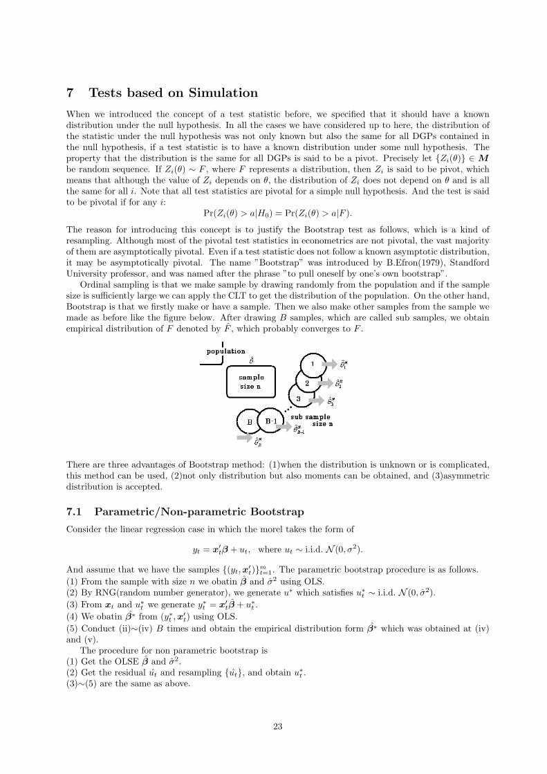
Ordinal sampling is that we make sample by drawing randomly from the population and if the samplesize is sufficiently large we can apply the CLT to get the distribution of the population. On the other hand,Bootstrap is that we firstly make or have a sample. Then we also make other samples from the sample wemade as before like the figure below. After drawing B samples, which are called sub samples, we obtainempirical distribution of F denoted by F , which probably converges to F .
There are three advantages of Bootstrap method: (1)when the distribution is unknown or is complicated,this method can be used, (2)not only distribution but also moments can be obtained, and (3)asymmetricdistribution is accepted.
7.1 Parametric/Non-parametric Bootstrap
Consider the linear regression case in which the morel takes the form of
yt = x′tβ + ut, where ut ∼ i.i.d. N (0, σ2).
And assume that we have the samples (yt,x′t)m
t=1. The parametric bootstrap procedure is as follows.(1) From the sample with size n we obatin β and σ2 using OLS.(2) By RNG(random number generator), we generate u∗ which satisfies u∗t ∼ i.i.d. N (0, σ2).(3) From xt and u∗t we generate y∗t = x′tβ + u∗t .(4) We obatin β∗ from (y∗t ,x′t) using OLS.(5) Conduct (ii)∼(iv) B times and obtain the empirical distribution form β∗ which was obtained at (iv)and (v).
The procedure for non parametric bootstrap is(1) Get the OLSE β and σ2.(2) Get the residual ut and resampling ut, and obtain u∗t .(3)∼(5) are the same as above.
23
7.2 Bootstrap test
As well as obtaining the distribution of estimator, we can obtain the distribution of statistic by Bootstrapmethod. Now let τ∗i be the ith value of τ . Define:
τ∗i :=β∗i − βi√Var(β∗i )
, F ∗(τ) =1B
B∑
i=1
I(τ∗i < τ),
where I(τ∗i < τ) is the indicator function which is one if the condition is met and is zero otherwise.When considering the lower 100α %, F ∗(τ) = α, and τ satisfies αB =
∑Bi=1 I(τ∗i ) is a critical point. For
replication number B, in order that α(B + 1) is integer, the optimal values are
α = 0.05 =⇒ 19, 39, 59,
α = 0.01 =⇒ 99, 199, 299.
By the construction of the distribution, the p value of a test is given by:
p(x∗) = 1− F (x∗)
= 1− 1B
B∑
i=1
I(xi ≤ x∗) =1B
B∑
i=1
I(xi > x∗).
Compared with asymptotic test, Bootstrap test have the characteristics in that size(:type I error) is betterthan asymptotic test and that power is lower a little.
8 Non Linear Model
Up to this point, we considered the linear regression model, which is given by:
yt = x′tβ + ut, where xt = (x1t · · ·xkt), ut ∼ i.i.d.(0, σ2).
For each observation t of any regression model, there is an information set Ωt and a suitably chosen vectorxt of explanatory variables that belong to Ωt. But although the elements of xt may be nonlinear function ofthe variables originally used to define Ωt, many types of nonlinearity cannot be dealt with by the frameworkof linearity. In this chapter we consider the nonlinear regression model, which takes the form of:
yt = xt(β) + ut, where ut ∼ i.i.d.(0, σ2).
Here xt(β) means that xt is characterized by parameters β and is called a nonlinear regression function.Hence we can write as xt(β) = g(xt,β) where xt ∈ Ωt. For example, g(x1t, x2t, β1, β2) = β1x
−β21t x2t.
Another way to write the nonlinear regression model is y = x(β) + u where u ∼ i.i.d.(0, σ2I).
8.1 The method of moments estimator and its property
As well as linear regression model, the orthogonal condition is imposed. For any k-dimensional vectorwt ∈ Ω, we have the moment conditions:
E(wtut) = 0.
Now let W be an n × k matrix, which takes the form of W = (w1 · · ·wn)′. Then the moment conditioncan be rewritten as:
n−1W ′u = n−1W ′(y − x(β))
= 0,
where x(β) = (x1(β) · · ·xn(β))′. Therefore the MM estimation of β is β such that n−1W ′(y − x(β))
=0. How we should choose W ? There are infinitely many possibilities. Using almost any matrix W ,of which the tth row depends only on variables that belong to Ωt and which has full column rank kasymptotically, yields a consistent estimator of β. These estimators, however, in general have differentasymptotic covariance matrices and it is therefore of interest to see if any particular choice of W leads toan estimator with smaller asymptotic variance than the others.
24
8.2 The concept of identification
Before analyzing the property of β which is the MM estimator of β, we consider the identification of β.The concept of identification is defined as follows:
Definition: By a given data set and a given estimation method, if we can obtain the unique parameter,then this parameter is said to be identified.Definition: As n →∞, if a parameter is identified then this parameter is said to be asymptotic identified.
Note that these two concepts of identification are not always on the inclusion relation. Define α(β) by:
α(β) := plim n−1W ′(y − x(β)).
Since a law of large numbers can be applied to the right hand side of the equation above, whatever thevalue of β is, α(β) is deterministic. If the DGP is y = x(β0) + u then we have:
n−1W ′(y − x(β))
= n−1W ′u = n−1n∑
t=1
Wtutp−→ 0.
Therefore we obtain the condition on which the asymptotic identification holds. In othere words, theparameter vector β is asymptotically identified, if β0 is the unique solution to the equations α(β) = 0.
α(β) = 0 for β = β0,
α(β) 6= 0 for β 6= β0.
8.3 The consistency of the NLE
The MM estimator is consistent estimator. An informal proof is given as follows.Under the finite sample number n, if β is identified, such a β is obtained that
n−1W ′(y − x(β))
= 0. (14)
Now let plim β = β∞, where β∞ 6= β0 and β∞ is not stochastic but constant. Then for the left hand sideof Eq.(14), consider its probability limit we have:
α(β∞) = plim n−1W ′(y − x(β∞))
= 0.
β0 is such that n−1W ′(y − x(β))
= 0 and we have shown that plim n−1W ′(y − x(β∞))
= 0. Howeverthis violates that β∞ 6= β0, which is a contradiction. Thus β∞ = β0, that is, β converges in probabilityto β0. Next consider the neccesary condition for asymptotic identification and consistency. Now we have:
α(β) = plim n−1W ′(y − x(β))
= plim n−1W ′(x(β0) + u− x(β))
= α(β0) + plim n−1W ′(x(β0)− x(β)),
where α(β0) = 0 by its definition. Therefore the necessary condition for asymptotic identification andconsistency is
plim n−1W ′(x(β0)− x(β)) 6= 0 for β 6= β0.
Hence we immediately obtain if β1 6= β0 then x(β1) 6= x(β0).
8.4 Asymptotic normality and asymptotic efficiency
By the mean value theorem, we can write x(β) as:
x(β) = x(β0) +∂x(β∗)
∂β′(β − β0), (15)
25
where β∗ is between β and β0 and (i, j) element of ∂x/∂β′ for i = 1, · · · , n and j = 1, · · · , k is given by∂xi(β)/∂βj . Henceforth we denote ∂x/∂β′ by X(β). Here the condition for MM implies that
n−1W ′(y − x(β))
= 0, for all n.
Multiplying both sides by√
n and inserting Eq.(15) into this, we obtain:
n−1/2W ′(y − x(β))
= n−1/2W ′(y − x(β0)−X(β0)(β − β0))
= n−1/2W ′u− n−1/2W ′X(β0)(β − β0))
= n−1/2W ′u− n−1W ′X(β0)√
n(β − β0) = 0 a.e,
(16)
where X(β∗) converges in probability to X(β0) and the notation a.e means almost everywhere. Thisfollows from the fact that since β converges in probability to β0, so does β∗. Let us define SW ′X to be:
plim n−1W ′X(β0) = lim n−1W ′E(X(β0)) := SW ′X . (17)
This equality is derived from applying a law of large numbers to n−1W ′X0. Under reasonable reguralityconditions, this holds. Then we have from Eq.(16) and Eq.(17):
√nSW ′X(β − β0) =
1√n
W ′u a.e.
Assume that SW ′X is full rank(: strong asymptotic identification) then the inverse matrix of SW ′X existsand noting that u
d→ N (0, σ2I), we get:
√n(β − β0) = n−1/2
(SW ′X
)−1
W ′u
d−→ N(0, σ2
0S−1W ′XSW ′W
(S−1
W ′X
)′),
where SW ′W := plim n−1W ′W and σ20 := E(u2
t ). The variance term is obtained from the calculation asfollows:
Var(n−1/2
(SW ′X
)−1
W ′u)
=(n−1S−1
W ′XW ′W (S−1W ′X)′
)σ2
= SW ′X(n−1W ′W )SW ′Xσ2 p−→ S−1W ′XSW ′W (S−1
W ′X)′σ2.
Analyzing the asymptotic variance of β, then we find that
σ20S−1
W ′XSW ′W
(S−1
W ′X
)= σ2
0plim(
n−1W ′X0
)−1(n−1W ′W
)−1(W ′X0
)−1
= σ20plim
n−1X ′
0W(W ′W
)−1
W ′X0
−1
= σ20plim
(n−1X ′
0PW X0
)−1
,
where X0 := X(β0) and PW is the orthogonal projection onto ℘(W ), the subspace spanned by thecolumns of W . If W = X0 then β is more efficient than any other estimators using W 6= X0. Thus,although X(β0) yields the most efficient one but it cannot be used actually.
8.5 Non linear least square
In the nonlinear regression model we can use the concept of least square, which is applied as:
β = arg minβ
(y − x(β)
)′(y − x(β)
).
The FOC to minimize is given by: (∂x(β)∂β′
)′(y − x(β)
)= 0.
This is identical to the case in which W = X(β) so that similarily consistency and asymptotic normalityhold, which states that √
n(β − β) d−→ N (0, σ20S−1
X′X).
26
8.6 Newton’s method
When considering the nonlinear model y = x(β)+u, where β is a k-dimensional vector, one way to obtainβ is numerical optimization. Applying to general case, we consider the optimization problem of Q(β).Letting the initial value of β be β0, by the second order Taylor expansion around β0, we can representQ(β) as: 5)
Q(β) = Q(β0) +∂Q(β0)
∂β′(β − β0) +
12(β − β0)′
∂2Q(β∗)∂β∂β′
(β − β0),
where β∗ is between β and β0. Here let us define Q#(β) to be approximation of the equation above:
Q#(β) = Q(β0) +∂Q(β0)
∂β′(β − β0) +
12(β − β0)′
∂2Q(β0)∂β∂β′
(β − β0). (18)
Then instead of the optimization problem of Q(β), we consider the optimization problem of Q#(β), ofwhich FOC is given by:
∂Q#(β)∂β
=∂Q(β0)
∂β+
12× 2
∂2Q(β0)∂β∂β′
(β − β0) = 0 ∴ ∂Q(β0)∂β
+∂2Q(β0)∂β∂β′
(β − β0) = 0.
where the first term of Eq.(18) becomes zero if being differentiated with respect to β since it is a functionof β0. Hence, if ∂2Q(β0)/∂β∂β′ is non singular, using this FOC, we obtain:
β − β0 = −(∂2Q(β0)
∂β∂β′
)−1 ∂Q(β0)∂β
.
And recursively, letting βj be the value by jth recursive calculation, we obtain:
βj+1 = βj −(∂2Q(βj)
∂β∂β′
)−1 ∂Q(βj)∂β
∴ βj+1 = βj −H(βj)−1g(βj),
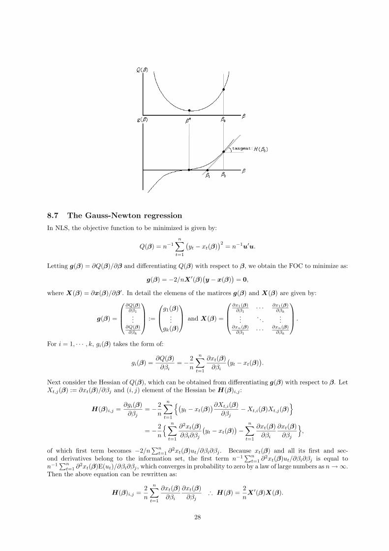
where we denote ∂2Q(βj)/∂β∂β′ by H(βj) and ∂Q(βj)/∂β by g(βj).This method can be understood by the figure below. If the quadratic approcimation Q](β) is a strictly
concave function, which it is if and only if the Hessian H(βj) is positive definite then βj+1 is the globalminimum of Q](β). And if Q](β) is a desirable approximation to Q(β), βj+1 should be close th thetrue minimum value for Q(β). But to use this method, we set the stopping rule, which is the level ofconvergence. The rule is generally given by:
g′(βj)H(βj)−1g(βj) < ε.
Ususally we set the convergence tolerance ε to be between 10−12 and 10−4. Of course, any stopping rulemay work badly if ε is chosen incorrectly, If ε is too large then the algorithm may stop soon. On the otherhand, if ε is too small, the algorithm may keep going long after βj is close enough to β.
There are disadvantages of Newton’s method: (1)if g(β) is not steep but flat locally, the optimum doesnot converge, (2)if an initial value is far from the optimum, it does not converge. Therefore it is importantto determine an initial value. To these disadvantages, the actions following are conducted: (1)an unbiasedestimator or consistent estimator is used as initial value since they probably converge to the true value ifthe sample number is sufficienly large and (2)the grid search method is conducted.
5)Q(˛) is assumed to be twice continuously differentiable and ∂Q(˛)/∂Q˛ has a typical element ∂Q(˛)/∂βi and
∂2Q(˛)/∂˛∂˛′ has a typical element ∂2Q(˛)/∂βi∂βj for i = 1, · · · , k and j = 1, · · · , k.
27
8.7 The Gauss-Newton regression
In NLS, the objective function to be minimized is given by:
Q(β) = n−1n∑
t=1
(yt − xt(β)
)2 = n−1u′u.
Letting g(β) = ∂Q(β)/∂β and differentiating Q(β) with respect to β, we obtain the FOC to minimize as:
g(β) = −2/nX ′(β)(y − x(β)
)= 0,
where X(β) = ∂x(β)/∂β′. In detail the elemens of the matirces g(β) and X(β) are given by:
g(β) =
∂Q(β)∂β1...
∂Q(β)∂βk
:=
g1(β)...
gk(β)
and X(β) =
∂x1(β)∂β1
· · · ∂x1(β)∂βk
.... . .
...∂xn(β)
∂β1· · · ∂xn(β)
∂βk
.
For i = 1, · · · , k, gi(β) takes the form of:
gi(β) =∂Q(β)
∂βi= − 2
n
n∑t=1
∂xt(β)∂βi
(yt − xt(β)
).
Next consider the Hessian of Q(β), which can be obtained from differentiating g(β) with respect to β. LetXt,j(β) := ∂xt(β)/∂βj and (i, j) element of the Hessian be H(β)i,j :
H(β)i,j =∂gi(β)∂βj
= − 2n
n∑t=1
(yt − xt(β)
)∂Xt,i(β)∂βj
−Xt,i(β)Xt,j(β)
= − 2n
n∑t=1
∂2xt(β)∂βi∂βj
(yt − xt(β)
)−n∑
t=1
∂xt(β)∂βi
∂xt(β)∂βj
,
of which first term becomes −2/n∑n
t=1 ∂2xt(β)ut/∂βi∂βj . Because xt(β) and all its first and sec-ond derivatives belong to the information set, the first term n−1
∑nt=1 ∂2xt(β)ut/∂βi∂βj is equal to
n−1∑n
t=1 ∂2xt(β)E(ut)/∂βi∂βj , which converges in probability to zero by a law of large numbers as n →∞.Then the above equation can be rewritten as:
H(β)i,j =2n
n∑t=1
∂xt(β)∂βi
∂xt(β)∂βj
∴ H(β) =2n
X ′(β)X(β).
28
The Gauss-Newton method gives its algorithm as:
βj+1 = βj −(H(βj)
)−1g(βj)
∴ βj+1 − βj = −(2/nX ′(βj)X(βj)
)−1g(βj)
= −(2/nX ′(βj)X(βj)
)−1(− 2/nX ′(βj)(y − x(βj)
))
=(X ′(βj)X(βj)
)−1X ′(βj)
(y − x(βj)
).
Notice that the right hand side of the equation above has the form of OLSE. Let b = βj+1 − βj then b isthe OLSE of the linear regression model of the form:
y − x(βj) = X(βj)b + res. (19)
Thus the updation of the value of βj+1 from βj is conducted by following the regression above. b isthe OLSE of Eq.(19), which is called Gauss-Newton regression, denoted simply GNR6) . Then why dowe use GNR? There are two reasons. Firstly, GNR confirmes whether or not NLS satisfies the FOCX ′(β)
(y−x(β)
)= 0. Secondly, GNR enables us to estimate the variance of β because Var(βj+1) = Var(b)
holds, which is followed by that since βj+1 = βj + bj and at j we know βj so that βj can be seen asconstant. Now, since we have b =
(X ′(β)X(β)
)−1X ′(β)
(y − x(β)
), we find:
E(b) = 0,
Var(b) = E(bb′) =(X ′(β)X(β)
)−1X ′(β)E(uu′)X(β)
(X ′(β)X(β)
)−1
=(X ′(β)X(β)
)−1X ′(β)ΩX(β)
(X ′(β)X(β)
)−1,
where Ω is called heteroskedasticity consistent covariance matrix estimator(:HCCME) and is given byΩ = diag
(E(u2
1), · · · ,E(u2n)
). The form of Ω means that u is heteroskedastic.
If we apply this logic to the function Q(β1,β2) of the form:
Q(β1,β2) = n−1n∑
t=1
(yt − xt(β1,β2)
)2,
then, letting β = (β′1β′2)′ and b = (b′1b
′2)′, the corresponding GNR is given by:
yt − xt(β) =∂xt(β)
∂β′b + res ∴ yt − xt(β) =
(∂xt(β)∂β′1
∂xt(β)∂β′2
)(b1
b2
)+ res
=∂xt(β1,β2)
∂β′1b1 +
∂xt(β1,β2)∂β′2
b2 + res.
9 Generalized Least Squares
9.1 Basic idea of GLS
If the parameters of a regression model are to be estimated efficiently by least squares, the error termsmust be uncorrelated and have the homoskedastic variance. These assumptions are needed to prove theGauss-Markov Theorem. But it is clear that we need new estimation methods to conduct regression of themodels with error terms that are heteroskedastic, serially correlated or both. Let us consider the regressionmodel which takes the form of y = Xβ + u, where E(u|X) = 0 and E(uu′|X) = Ω, which is the n × nsymmetric, positive definite matrix. The diagonal elements of Ω are not constant, thus u is heteroskedasticand the off-diagonal ones are not zero, thus u is serially correlated. In this case, the OLSE β is unbiased,however, it is not efficient since
Var(β|X) = (X ′X)−1X ′E(uu′|X)X(X ′X)−1
= (X ′X)−1X ′ΩX(X ′X)−1.6)
This regression is ”artificial” because the variables that appear in it are not the explained and explanatory variables ofthe nonlinear regression.
29
Then how can we obtain the efficient estimator? Here consider the matrix Ψ7) such that ΨΩΨ′ = σ2I.Premultiplying the model above by Ψ′, we have:
Ψ′y = Ψ′Xβ + Ψ′u,
of which OLS estimator βGLS is obtained as:
βGLS =((Ψ′X)′(Ψ′X)
)−1(Ψ′X)′(Ψ′y)
= (X ′ΨΨ′X)−1(X ′ΨΨ′y) = β + (X ′ΨΨ′X)−1(X ′ΨΨ′u).
Then the expectation and the variance of βGLS are given by:
E(βGLS|X) = β,
Var(βGLS) = (X ′ΨΨ′X)−1X ′ΨΨ′E(uu′|X)ΨΨ′X(X ′ΨΨ′X)−1
= (X ′ΨΨ′X)−1X ′Ψ(σ2I)Ψ′X(X ′ΨΨ′X)−1 = σ2(X ′ΨΨ′X)−1.
By the way, how can we get Ψ? In order to get it, we need to have the knowledge about eigen value andeigen vector 8) . For Ωxi = λixi, premultiplying both sides by x′i and x′i with i 6= j, respectively, wehave9) :
x′iΩxi = λix′ixi = λi and x′jΩxi = λjx
′jxi = 0.
Then using these relation, and letting Γ := (x1 · · ·xk) and Λ := diag(λ1 · · ·λk), we get:
Γ′ΩΓ = Λ.
Thus noting that ΓΓ′ = I = Γ′Γ, we have:
Ω = (Γ′)−1ΛΓ−1 = ΓΛΓ′, ∴ Ω−1 = ΓΛ−1Γ′.
By these equations we immedialtely obtain ΩΩ−1 = ΓΛΓ′ · ΓΛ−1Γ′ = I and therefore we find:
Ω−1 = ΓΛ−1Γ′ = (ΓΛ−1/2)(Λ−1/2Γ′) = ΨΨ′.
9.2 Geometry of GLSE
Since βGLS = (X ′Ω−1X)−1(X ′Ω−1y), the fitted values from the GLS regression are given by:
y = XβGLS = X(X ′Ω−1X)−1(X ′Ω−1y).
Hence tha matrix that projects y onto ℘(X) and its contenporary projection matrix are, respectively:
P ΩX = X(X ′Ω−1X)−1X ′Ω−1,
MΩX = I − P Ω
X = I −X(X ′Ω−1X)−1X ′Ω−1.
These are not symmetric but idempotent since
P ΩXP Ω
X = X(X ′Ω−1X)−1X ′Ω−1 ·X(X ′Ω−1X)−1X ′Ω−1 = X(X ′Ω−1X)−1X ′Ω−1,
MΩXMΩ
X = (I − P ΩX )(I − P Ω
X ) = I − P ΩX = MΩ
X .
However, as they are not symmetric, P ΩX does not project orthogonally onto ℘(X) and MΩ
X projects onto℘⊥(Ω−1X) rather tan ℘⊥(X). They are examples of what we call oblique projection matrices because theangle between the residuals MΩ
Xy and the fitted value P ΩXy is in general not 90. This is because
(P ΩXy)′MΩ
Xy = y′Ω−1X(X ′Ω−1X)−1X ′(I −X(X ′Ω−1X)−1X ′Ω−1)y
= y′Ω−1X(X ′Ω−1X)−1X ′y − y′Ω−1X(X ′Ω−1X)−1X ′X(X ′Ω−1X)−1X ′Ω−1y,
which is equal to zero only in certain very special cases such as when Ω is proportional to I. Thus GLSresiduals are in general not orthogonal to GLS fitted values.
7)Ψ is usually triangular matrix.
8)If there exists non zero vector x such that Ωx = λx for λ then λ is called eigen value and x is said to be eigen vector
corresponding to λ. Note that the number of eigen value which is not zero is equalt to rank(X). Ususally the norm of aneigen vector is standarized to one. And letting xi be the eigen vector corresponding to λi and xj be the one correspoindingto λj then x′ixj = 0 for i 6= j.
9)This is only if Ω is symmetric.
30
9.3 Interpretting GLSE
Firstly GLSE can be seen as the OLSE of the model Ψ′y = Ψ′Xβ + Ψ′u, where E(uu′) = σ2Ω andΩ−1 = ΨΨ′. In this model we can obtain the GLSE as:
βGLS = (X ′ΨΨ′X)−1(X ′ΨΨ′y)
= (X ′Ω−1X)−1(X ′Ω−1y)
= (X ′Ω−1X)−1X ′Ω−1(Xβ + u)
= β + (X ′Ω−1X)−1(X ′Ω−1u),
which implies that βGLS is unbiased estimator. And its variance is given by:
Var(βGLS|X) = (X ′ΨΨ′X)−1X ′ΨΨ′E(uu′|X)ΨΨ′X(X ′ΨΨ′X)−1
= (X ′ΨΨ′X)−1X ′Ψ(σ2I)Ψ′X(X ′ΨΨ′X)−1 = σ2(X ′ΨΨ′X)−1 = σ2(X ′Ω−1X)−1.
Since βGLS satisfies the basic assumptions for OLSE to be BLUE, it is also BLUE. Further more, βGLS ismore efficient than βOLS. Since Var(βGLS) = σ2(X ′Ω−1X)−1 and Var(βOLS) = σ2(X ′X)−1X ′ΩX(X ′X)−1,we have:
σ−2(Var(βOLS −Var(βGLS)
)= (X ′X)−1X ′ΩX(X ′X)−1 − (X ′ΩX)−1
=(X ′X)−1X ′)Ω(
X ′X)−1X ′)′ − (X ′ΩX)−1X ′Ω−1ΩΩ−1X(X ′ΩX)−1
=(X ′X)−1X ′)Ω(
X ′X)−1X ′)′ − ((X ′Ω−1X)−1X ′Ω−1
)Ω
((X ′Ω−1X)−1X ′Ω−1
)′
=((X ′X)−1X ′ − (X ′Ω−1X)−1X ′Ω−1
)Ω
((X ′X)−1X ′ − (X ′Ω−1X)−1X ′Ω−1
)′,
which is positive definite and means that βGLS is more efficient than βOLS. Secondly consider minimizingthe GLS criterion function of the form:
βGLS = arg minβ
(Ψu)′(Ψu) = u′Ω−1u
= (y −Xβ)′Ω−1(y −Xβ),
of which FOC is given by X ′Ω−1(y−Xβ) = 0. Letting W = Ω−1X then this is identical to the momentcondition. If (W ′X)−1 exists then the MM estimator βMM is βMM = (W ′X)−1Wy, which implies that
βMM = β + (W ′X)−1W ′u.
The GLS estimator is evidently a special case of this MM estimator with W = Ω−1X. Therefore itsconditional expectation and variance given X and W are
E(βMM|X,W ) = β,
Var(βMM|X,W ) = (W ′X)−1W ′ΩW (X ′W )−1.
The situations which need GLS are i: the error terms have heteroskedastic variance, ii: the error terms areserially correlated, and iii: panel data(random effect model).Note that if E(uu′) = Ω = σ2∆ where σ2 is unknown and ∆ is known then by the Cholesky decompositionof ∆ we can do as well as above. And if Ω is known then GLSE is efficient and even if it is unknown thenGLSE is asymptotically efficient.
9.4 Heteroskedasticity
It is easy to obtain GLS estimator when the error terms are heteroskedastic but uncorrelated. If the form ofΩ is known, that is, if Ω = diag(ω2
1 , · · · , ω2n) then Ω−1/2 = diag(ω−1
1 , · · · , ω−1n ). In this case the regression
of the form:Ω−1/2y = Ω−1/2Xβ + Ω−1/2u.
31
is called weighted least squares(:WLS), of which estimator βWLS is given by:
βWLS =((Ω−1/2X)′(Ω−1/2X)
)−1(Ω−1/2X)′(Ω−1/2y) = (X ′Ω−1X)−1(X ′Ω−1y).
Thus the expecation and the variance of the error term are:
E(Ω−1/2u) = 0,
Var(Ω−1/2u) = E(Ω−1/2uu′Ω−1/2)
= Ω−1/2E(uu′)Ω−1/2 = Ω−1/2ΩΩ−1/2 = I.
Next we consider the case in which Ω is unknown but can be formulated, that is, for some scalar functionh(·) 10) , E(u2
t ) take the form of:E(u2
t ) = h(δ + Z ′tγ),
where δ is a scalar and Zt and γ are r-dimensional vectors 11) . Then ut2 can be formulated as 12) :
u2t = h(δ + Z ′
tγ) + νt.
We can test the null hypothesis that γ = 0 by using GNR. The GNR corresponding to the above model is
u2t − h(δ + Z ′
tγ) = h′(δ + Z ′tγ)bδ + h′(δ + Z ′
tγ)Z ′tbγ + error,
where h′(·) is the first derivative of h(·). And bδ and bγ are the coefficients which should be estimated andare corresponding to δ and γ. In detail in the above equation, the coefficients on bδ and bγ are respectivelyequal to h′(·)∂(δ + Z ′
tγ)/∂δ and h′(·)∂(δ + Z ′tγ)/∂γ. Evaluating at γ = 0 then we can simplify this GNR
to:
u2t − h(δ) = h′(δ)bδ + h′(δ)Z ′
tbγ + error= h′(δ)bδ + Z ′
th′(δ)bγ + error,
∴ u2t = b∗δ + Z ′
tb∗γ + error,
where b∗δ := h(δ) + h′(δ)bδ and b∗γ := h′(δ)bγ . Since h(δ) and h′(δ) are just a constant, the form of thisfunction does not depend on h(·). In practice, we do not actually observe the ut. However, as we knowthat least squares residuals converge asymptotically to the corresponding error terms when the model iscorrectly specified, it seems plausible that the test should still be asymptotically valid if we replace u2
t inthe regression. Hence the test regression becomes:
ut2 = b∗δ + Z ′
tb∗γ + error. (20)
We conduct the test for the null and the alternative hypothesis given by:
H0 : b∗γ = 0, H1 : b∗γ 6= 0.
Under the null hypothesis, nR2u follows χ2 distribution with r degrees of freedom, where R2
u is the determi-nation coefficient of Eq.(20). This test is called Breusch Pegan test. Other tests for checking heteroskedas-ticity are, say, White test and Goldfeld-Quandt test. Simply the proceduare is as follows: (1)get OLSE β,(2)get the residual ut = yt − x′tβ, (3)estimate the model ut = h(δ + Z ′
tγ) and get the initial value δ1 andγ1, (4)let wt =
(h(δ +Z ′
tγ))−1/2 and conduct WLS estimation then obtain βWLS and (5)return to (2) and
keep these proceduare until δ and γ converge.
10)The skedastic function h(·) is a nonlinear function that can take on only positive values.
11)Zt is a vector of observations on exogenous or predetermined variables that belong to the information set.
12)We cannot generally say that νt ∼ i.i.d.(0, σ2) because the distribution of u2
t will generally be skewed to the right. Butunder the null hypothesis ‚ = 0, it seems unreasonable to assume that the variance of νt is constant.
32
9.5 Serial correlation
The phenomenon of serial correlation means that error terms in a regression model are correlated. Serialcorrelation is very commonly encountered in applied work using time-series data. One of the simplest andthe most popular case with serial correlation is to assume that the error terms in the regression modelyt = x′tβ + ut follow the first-order autoregressive, denoted simply by AR(1), process of the form:
ut = ρut−1 + νt, where νt ∼ i.i.d.(0, ω2).
To begin with, we introduce the concept of covariance stationarity, or weak stationarity here.
Definition: A random sequence ut is said to be covariance stationary if E(ut) = µ and Var(ut) = σ2
for all t, which means that the expectation and the variance of ut are constant and if cov(ut, us) = γ|t−s|,which means that the covariance depends only on the difference between time period t and s.
Here we assume that E(ut) = 0 and |ρ| < 113) , then ut can be rewritten as:
ut = ρut−1 + νt
= ρ(ρut−2 + νt−1) + νt
= ρ2ut−2 + ρνt−1 + νt = · · · =∞∑
j=0
ρjνt−j .
Thus the variance of ut is obtained as:
Var(ut) = E( ∞∑
j=0
ρjνt−j
)2
=∞∑
j=0
ρjE(ν2t ) =
ω2
1− ρ2,
and the covariance between ut and ut−h is given by:
γh = E(utut−h) = E( ∞∑
j=0
ρjνt−j
∞∑
j=h
ρj−hνt−h−j
)= ρh
∞∑
j=0
ρ2jE(ν2t−j) =
ρhω2
1− ρ2.
Since ut follows AR(1) now, its variance-covariance matrix Ω is given by:
Ω =ω2
1− ρ2
1 ρ · · · ρn−1
ρ 1 · · · ρn−2
......
. . ....
ρn−1 ρn−2 · · · 1
:= ω2Ω∗.
For the matrix Ω∗, its Cholskey decomposition gives (Ω∗)−1 = LL′ so that the WLS is
L′y = L′Xβ + L′u ∴ βWLS = (X ′Ω−1X)−1X ′Ω−1y,
where the elements of the matrix L′ is as follows:
L′ =
(1− ρ2)1/2 0 · · · 0−ρ 1 · · · 0...
.... . .
...0 0 · · · 1
.
Notice that L′y has the first element√
1− ρ2y1 and the other elements yt − ρyt−1 for t = 2, · · · , n.The transformation using both the first element
√1− ρ2y1 and the other elemet is called Prais-Winsten
transformation and the one not using the first elemtent is called Cochran-Orcutt transformation.13)
In AR(1) process, |ρ| < 1 is the necessary and sufficient condition on which covariance stationarity is met. If ρ = 1 thenut is said to follow random walk. This process is that the influence from the past values does not diminish but has influenceon the present value.
33
To test whether or not the first-order serial correlation is presented, we can use Durbin-Watson test, ofwhich test statistic is defined as:
DW :=∑n
t=2(ut − ut−1)2∑nt=1 ut
2∼= 2(1− ρ),
where the last asymptotice equality holds if we ignore the difference between∑n
t=1 ut2 and
∑nt=2 u2
t−1.Thus in the sample of reasonable size a value of DW equals to 2 if serial correlation is not presented. Butthere are problems of this test. Firstly, this test can be applied to only the serial correlation with firs-order.Thus if we need to test whether or not a higher order serial correlation, say, ut = ρ1ut−1 +ρ2ut−2, this testis useless. Secondly if the regreesion model has lagged variables, this test cannnot be used. For instance,to the regression model yt = β1yt−1 + ut, we cannnot use this test.
In order to resolve these problems we use other test. Consider the case in which the regression model isyt = x′tβ + ut and we need to confirm whether or not ut follows AR(1). By the condition we immediatelyget:
yt = ρyt−1 + x′tβ − ρx′t−1β + νt.
Then the corresponding GNR is given by:
yt − ρyt−1 − x′tβ + ρx′t−1β = (x′t − ρx′t−1)b + bρ(yt−1 − x′t−1β) + νt.
The first regressor is the derivative of the regression function with respect to β and the second regressoris the one with respect to ρ. Under the null hypothesis H0 : ρ = 0, which implies that ut is seriallyuncorrelated, the above model can be rewritten as:
yt − x′tβ = x′tb + bρ(yt−1 − x′t−1β) + νt.
Hence setting the null hypothesis that bρ = 0 and replacing ut = yt − x′tβ by ut we can conduct the test:
ut = x′tb + bρut−1 + error.
10 Analysis of Panel Data
Panel data sets are measured across two dimenstions. One dimension is time and the other is usually calledthe cross-section dimenstion. For exmaple, it is the case in which we have 40 annual observations on 25countries. The typical model for panel data is written as:
yit = x′itβ + uit, for i = 1, · · · ,m, t = 1, · · · , T.
In matrices form, the above model can be written as y = Xβ + u where y is an n = mT -dimensionalvector, X is an n×m matrix and β is an m-dimensional vector and u is an n-dimensional vector with theelements of the matrices are given by:
y =
y1
...ym
, where yi =
yi1
...yiT
; X =
x11 · · · xm1
.... . .
...x1m · · · xmm
, where xit =
xi1
...xiT
;u =
u1
...um
where ui =
ui1
...uiT
.
As the model above indicate, there are m cross-sectional samples and T time periods for a total of n = mTobservations. For analysis, we assume firstly that uit ∼ i.i.d.(0, σ2). Under this assumption, we can saythat E(uitujs) = 0 for all t 6= s and i 6= j, and can conduct OLS regression, which is especially calledpooling regression. But there are some problems. They are that, although heteroskedasticity may bepresented, it is ignored and that time effect is ignored. If certain shocks affect the same cross-sectional unitat all points in time, the error terms uit and uis must be correlated for all t 6= s. And if certain shockesaffect all cross-sectionaly units at the same point in time then uit and ujt are correlated for all i 6= j.
If we ignore these probmes and conduct OLS regression, the result of this regression have the problemthat the OLSE is not efficient and that the variance covariance matrix of the error term is not consistent.Hence we here need to model the structure of uit. The typical modeling of uit is
uit = et + νi + εit,
34
which is usually called error component model. Here et is time effect, which affects all observations for timeperiod t, νi is individual effect, which affects all observations for cross-sectional unit i and εit is randomeffect, which affects only observation it. Each of them is assumed to be uncorrelated of the others. It isgenerally assumed that et is independent across t, νi is independent across i and εit is independent acrossall i and t.
10.1 Fixed effect model
A common formulation of the fixed model assumes that differences across units can be captured in differ-ences in the constant term. In this fixed effect modeling, we regard et and νi as the population parameters,that is, if et and νi are thought of as fixed then they are treated as the parameters to be estimated. Foridntification
∑t et = 0 and
∑i νi = 0 are assumed. To estimat the fixed effect model, we let et = 0 and
consider the regression with dummy variable:
y = Xβ + Dη + ε, where E(εε′) = σ2ε I, (21)
where y is an n-dimensional vector, D is an n×m matrix, η is an m-dimensional and ε is an n-dimensionalvector. Here let us define the projection matrix PD and MD to be:
PD := D(D′D)−1D′ and MD := I − PD.
Here the matrix D and PD are given by:
D =
ı 0 · · · 00 ı · · · 0...
.... . .
...0 0 · · · ı
and PD = T−1
ıı′ 0 · · · 00 ıı′ · · · 0...
.... . .
...0 0 · · · ıı′
since D′D = TIm,
where ı is a T -dimensional vector and there are m ıs in each columns of D. Then the FLW theoremimplies that the OLSE of Eq.(21) is identical to that of the following model:
MDy = MDXβ + MDε,
where MDy has the typical element yit − yt and yt is the group mean given by yt = T−1∑T
t=1 yit. Thusthis estimation means the regression of yit − yt on xit − xit. Then the OLSE is given by:
βFE = (X ′MDX)−1X ′MDy,
which is unbiased and BLUE because X and D are exogenous and of which variance is obtained as:
Var(βFE) = σ2ε (X ′MDX)−1.
Since all the variables in βFE are premultiplied by MD, it follows that this estimator makes use only ofthe information in the variation around the mean for each of the m groups. For this reason, it is oftencalled within-group estimators.
10.2 Random effect model
The fixed effects model is a reasonable approach when we can be confident that the differences betweenunits can be viewd as parametoric shifts of the regression function. This model might be viewed as applyingonly to the cross sectional units in the study, not to additional ones outside the sample. In this modeling14)
we regard et and νi as random variables such that et ∼ (0, σ2e) and νi ∼ (0, σ2
ν). We here need to figureout the covariance matrix of the uit as functions of the variances of the et, νi and εit. We assume thatthe matrix X of explanatory variables and the cross-sectional errors νi should both be independent ofεit but this does not rule out the possibility of a correlation between them. Also we impose on νi to be
14)In addition fixed effect modeling and randome effect modeling, we can use mixed effect modeling. This modeling is
mixture of fixed and random effect modeling, say, et is fixed and νi is random.
35
independent of X.Consider the OLS regression of the form:
PDy = PDXβ + error,
which immediately yields the OLSE as:
βRE = (X ′PDX)−1X ′PDy.
Since error = PD(v + ε), its elements are given by:
PD(ν + ε) = T−1
11′ 0 · · · 00 11′ · · · 0...
.... . .
...0 0 · · · 11′
ν1
...νm
+ T−1
11′ 0 · · · 00 11′ · · · 0...
.... . .
...0 0 · · · 11′
ε1
...εm
,
where νi is a T -dimensional vector such that νi = (νi · · · νi)′ and εi is also a T -dimensional vector suchthat εi = (εi1 · · · ε′iT ). Then PD(ν + ε) can be simplified to:
PD(ν + ε) = T−1
ıı′ν1
...ıı′νm
+ T−1
ıı′ε1
...ıı′εm
with ıı′νi = T
νi
...νi
and ıı′εi =
∑Tj=1 εij
...∑Tj=1 εij
.
Thus PD(ν + ε) is obtained as:
PD(ν + ε) = T−1T
ν1
...νm
+ T−1
ε∗1...
ε∗m
, where ε∗i =
∑Tj=1 εij
...∑Tj=1 εij
.
Hence the typical element of error is resit = νi + T−1∑T
j=1 εij so that its variance is
Var(resit) = E
(νi + T−1
T∑
j=1
εij
)2
= E(ν2i ) + T−2E
(T∑
j=1
εij
)2
= σ2ν + T−2
T∑
j=1
E(ε2ij) = σ2ν + T−2
T∑
j=1
σ2ε = σ2
ν + T−1σ2ε .
Here the pooling regression estimator is obtained as:
βPR = (X ′X)−1X ′y = (X ′X)−1X ′(MD + PD)y
= (X ′X)−1X ′MDy + (X ′X)−1X ′PDy
= (X ′X)−1X ′MDXβFE + (X ′X)−1X ′PDXβRE.
Next, to consider GLS, we let uit be uit = νi + εit and calculate the variance and the covariance as:
Var(uit) = σ2ν + σ2
ε , E(uituis) = σ2ν , for all t 6= s and E(uitujs) = 0, for all i 6= j.
Let ui = (ui1 · · ·uiT )′ then we obtain:
E(uiu′i) =
σ2u + σ2
ε σ2ν · · · σ2
ν
σ2ν σ2
ν + σ2ε · · · σ2
ν...
.... . .
...σ2
ν σ2ν · · · σ2
ν + σ2ε
= σ2
eI + σ2νıı′ = Σ,
36
where the diagonal elemets are all σ2u + σ2
ε and the off-diagonal ones are σ2ν . Then the mT -dimensional
vector u = (u1 · · ·um)′ satisfies:
Ω = E(uu′) =
Σ o. . .
o Σ
= Σ⊗ I.
In order to obtain GLS estimator of β, the values of σ2u and σ2
e or at least the ratio between them mustbe unknown. The GLS estimator of the random effect model can be obtained from the regressoin as:
(I − λPD)y = (I − λPD)Xβ + res,
where λ = 1 − (Tσ2ν/σ2
ε + 1)−1/2. This value is obtained as follows: since Σ = σ2ε I + σ2
νıı′, this can berewritten as:
Σ = σ2ε I + σ2
νıı′ = σε
(I +
σ2ν
σε11′
)= σ2
ε V , where V := I +σν
σε11′,
so that Σ−1/2 = σ−1ε V −1/2 and for some λ, V can be represented as V −1/2 = I−λP1, where P1 = T−1ıı′.
Then V −1 is obtained as:V −1 = (I − λP1)2 = I + (λ2 − 2λ)P1,
and, noting that P1 = T−111′, we have:
V −1V =(I + (λ2 − 2λ)P1
)(I +
σ2ν
σ2ε
11′)
= I +(σ2
ν
σ2ε
T + (λ2 − sλ) + (λ2 − 2λ)σ2
ν
σ2ε
))P1
= I +((a + 1)λ2 − 2(a + 1)λ + a
),
where a := T−1σ2ν/σ2
ε . Now it must hold that(((a + 1)λ2 − 2(a + 1)λ + a
)= 0, of which solution is
λ = 1−(Tσ2
ν
σ2ε
+ 1)−1/2
.
The GLS estimator is identical to the OLS estimator when λ = 0, which happens if σ2ν = 0 and is equal to
the fixed effect estimator when λ = 1, which happens if σ2e = 0.
Then are really νi and xt uncorrelated? If they are correlated, the β is not unbiased and inefficient.To deal with this problem, Hausman test is conducted. If νi and xit are uncorrelated, βFE and βGLS areboth biased. Since βGLS is BLUE, Var(βFE) is larger than Var(βGLS). The Hasuman test is conducted asfollows: (1)in order to define the test statistic, we set the matrix Φ as:
Φ := Var(βFE − βGLS) = Var(βFE)−Var(βGLS),
and (2)the test statistic is defined by:
w := (βFE − βGLS)′Φ−1(βFE − βGLS),
which follows χ2 distribution with k−1 degrees of freedom under the null hypothesis that cov(νi,xit) = 0.
11 Instrumental Variable Method
As before, we considered the case in which the assumptions as to the error term u are not met: Var(u|X) 6=σ2I in the model y = Xβ + u. In this case, the OLSE β is unbiased and consistent but not efficient. Inorder to deal with this problem, we have used GLS, which yields the BLUE. However, what if the otherassumtions E(u|X) = 0 are not met? In this case, the OLSE is no longer unbiased and consistent. Forthis problem, here we introduce Instrumental Variable method, denoted simply IV method.
If E(u|X) 6= 0 then cov(Xu′) 6= 0, thus, as stated above, the OLSE β is no longer consistent since:
plim βOLS = β +(plim n−1X ′X
)−1plim n−1X ′u,
37
and the third term n−1X ′u does not converges in probability to 0. Then what are the cases in whichE(u|X) = 0 is not met ? The following two cases are typical examples.
Error in variables: Many economic variables are measured with error. Measurement error in the depen-dent variable of a model are geerally of no great consequence, unless they are very large. But measurementerror in the independent variables cause the error terms to be correlated with the regressord being measuredwithe error and this causes OLS to be inconsistent. Consider the model below:
yt = β1 + β2xt + ut , where ut ∼ i.i.d.(0, σ2).
Here yt and xt are unobserved variables, which are represented as, by using proxy variables xt and yt:
xt = xt + v1t and yt = yt + v2t,
where E(vit) = 0 and E(v2it) = w2
i for i = 1, 2, cov(v1t, v2t) = 0 and v1t and v2t are independent of xt , ytand ut . Then the above model can be rewritten as:
yt = β1 + β2xt + ut + v2t − β2v1t
Letting ut := ut + v2t − β2v1t, we can get the variance of ut as:
Var(ut) = σ2 + w22 + β2
2w21.
The effect of the measurement error in the dependent variable is simply to increase the variance of theerror terms. And the measurement error in the independent variable also increases the variance of theerror terms, but it has another, much more severe consequences. Here we can get the covariance betweenxt and ut as:
cov(xt, ut) = E((xt − E(xt))ut
)
= E(xtE(ut|xt)
)
= E((xt + v1t)(ut + v2t − β2v1t)
)
= −β2E(v21t) = −β2w
21,
which is generally non-zero. Because xt = xt + v1t and ut depends on v1t, ut must be correlated with xt
whenever β2 6= 0. This fact can be confirmed by:
E(ut|xt) = E(ut|v1t) = −β2v1t.
Simultaneous Equations: This is the case in which 2 or more endogenous variables are determinedsimultaneously. In this case, all of ther endogenous variables must be correlated with the error. Letting pt
be price and qt be quantity, we consider the following demand function and supply function, which takethe form:
qt = rdpt + x′dtβd + udt : demand function,
qt = rspt + x′stβs + ust : supply function,
where xdt and xst are observations of exogenous or predetermined variables. These expression can berewritten in the matrix form:
(1 −rd
1 rs
)(qt
pt
)=
(x′dtβd
x′stβs
)+
(ud
t
ust
)∴
(qt
pt
)=
1rd − rs
(−rs rd
−1 1
)(x′dtβd + ud
t
x′stβs + ust
).
Thus pt can be obtained as:
pt =1
rd − rs
((−x′dtβd + x′stβs) + (−ud
t + ust )
).
As shown above, pt depends on both udt and us
t . Thus pt must be correlated with the error terms in bothof those equations. It is easy to see that, whenever we have a linear simultaneous equation model, theremust be correlations between all of ther error terms and all of ther endogenous variables.
38
11.1 IV estimator
We will focus on the model yt = x′tβ+ut with E(u2t ) = σ2, that is, with a homoskedastic variance. Suppose
that there exists or we found a k-dimensional vector Wt such that
E(ut|Wt) = 0, where Wt ∈ Ωt,
which can be applied to the expression cov(ut,Wt) = 0 or E(utWt) = 0. The Wt is called instrumentalvariable, denoted by IV. IV may be either exogenous or predetermined, and they should always includeany columns of X that are exogenous or predetermined. Here we can rewrite this expression as in thesample mean expression:
n−1n∑
t=1
Wt(yt − x′tβ) = 0 ∴n∑
t=1
Wtyt −( n∑
t=1
Wtx′t
)β = 0,
where∑n
t=1 Wtx′t is full rank. Hence we can obtain the IV estimator βIV as:
βIV =( n∑
t=1
Wtx′t
)−1( n∑t=1
Wtyt
)= (W ′X)−1Wy,
where the tth row of W is Wt. Next in order to analyze the properties of the IV estimator, we considerthe regression model y = Xβ + u with E(uu′) = σ2I. The moment condition above can be simplifiedinto:
W ′(y −Xβ) = 0.
Also βIV can be rewritten as:
βIV = (W ′X)−1W ′y = β + (W ′X)−1W ′y,
which means that βIV is consistent, if and only if plim n−1W ′u = 0, because
plim βIV = β +(plim n−1W ′X
)−1
plim n−1W ′u.
The necessary-sufficient condition plim n−1W ′u = 0 follows from the MM condition and implies that theerror terms are asymptotically uncorrelated with the instruments. And the asymptotic variance is givenby, since
√n(βIV − β) =
(plim n−1W ′X
)−1
plim n−1/2W ′u,
we get:
Var(√
n(βIV − β))
=(plim n−1W ′X
)−1(plim n−1W ′W)σ2
(plim n−1X ′W
)−1
= σ2((
n−1W ′X)′(
n−1W ′W)−1(
n−1W ′X))−1
= σ2(n−1X ′W (W ′W )−1W ′X
)−1 = σ2(n−1X ′PW X
)−1,
where PW := W (W ′W )−1W ′. If we have some choice over what instruments to use in the matrix W , itmakes sense to choose them so as to minimize the above asymptotic covariance matrix.
11.2 The number of IV and the identification
Consider the linear regression model y = Xβ + u and an n× l IV matrix W , which is defined as:
W :=
W ′1
...W ′
n
, where Wi =
w1
...wl
,
39
where Wi is an l-dimensional vector, l is the number of IVs and k is the number of parameters. Hence, asstated above, since the MM conditions are W ′(y−Xβ) = 0 which is an l-dimensional vector, l is also thenumber of MM conditions. The relation between k and l is summarized as follows:
If k > l then underidentification. In this case, IV method is useless.If k = l then just identification.
If k < l then overidentification. In this case, some devices are needed.
Then what do we need to deal with, in the overidentification case ? We use the generalized IV estimator,denoted by GIVE. Here let us introduce the matrix J , which is an l × k matrix with k < l. Then we usethe n×k matrix WJ as a new IV. We can always treat an overidentified model as if it were just identifiedby choosing exactly k linear combinations of the l columns of W . But the matrix J is such that
rank(J) = k, if not so, under identified,
J is asymptotically deterministic,
J is chosen to minimize Var(βIV) in the calss of IV estimators.
Then J is approximated as:J ' (W ′W )−1W ′X,
which is called first stage fitted values and can be seen as the OLSE of the regression X = WJ + V .Using WJ as IV instead of W , we can get the generalized IV estimater, denoted by βGIV, as:
βGIV =((WJ)′X
)−1(WJ)′y
= (X ′PW X)−1X ′PW y = β + (X ′PW X)−1X ′PW u,
and the variance of GIVE is obtained as:
Var(βGIV) = σ2(X ′PW X)−1,
which is identical to the variance of IV estimator in the case of just identification.
11.3 Testing based on IV
Test of overidentification: Since the case is overidentification, we henceforth consider the case of l > k.To conduct test, here we define the notation as follows: firstly, l− k is the degree of overidentification andWJ = PW X, which is called effective instruments and secondly W can be divided into two parts, WJand n× (l − k) matrix W ∗, which is called an extra instruments such that ℘(W ) = ℘(PW X,W ∗). Thismeans that the l dimensional span of the full set of instrument is generated by linear combination of theeffective instruments and the extra instruments. The overidentifying restriction requires:
E((W ∗)′u) = 0.
But since we do not observe u, we can estimate the vector u by the vector of IV residuals u:
n−1(W ∗)′u = 0.
The null and alternative hypotheses of this test are defined as:
H0 : y = Xβ + u, where u ∼ i.i.d.(0, σ2I), E(W ′u) = 0,
H1 : y = Xβ + W ∗γ + u, where u ∼ i.i.d.(0, σ2I), E(W ′u) = 0.
And the F test statistic is u′PW ∗u = u′W ∗((W ∗)′W ∗)−1(W ∗)′u. Since the middle matrix of thisstatistic is positive definite by construction, it can be seen that the F test is testing whether or notn−1(W ∗)′u is significantly different from 0.
40
Durbin-Wu-Hausman test: This is the test to confirm whether or not IV is needed when predeterminedinformation is not avairable. The null and alternative hypotheses for DWH test are defined by:
H0 : E(X ′u) = 0, and H1 : E(X ′u) 6= 0, E(W ′u) = 0.
Under H0 and H1, both βOLS and βIV are consistent. But while under H1, βIV is consistent, βOLS is notso. Hence under H0 it follows that
plim(βIV − βOLS
)= 0.
And for the latter argument, we rewrite the above equation as:
βIV − βOLS = (X ′PW X)−1X ′PW y − (X ′X)−1X ′y
= (X ′PW X)−1(X ′PW y − (X ′PW X)(X ′X)−1X ′y
)
= (X ′PW X)−1X ′PW
(I −X(X ′X)−1X ′)y
= (X ′PW X)−1X ′PW MXy,
where X ′PW X is positive definite by the identification condition. Hence, testing whethere or not βIV −βOLS is significantly different from zero, is equivalent to testing whether or not the matrix X ′PW MXy issignificantly different from zero. This argument is summarized as:
βIV − βOLS = 0 ∴ X ′PW MXy = 0
plim (βIV − βOLS) = 0 ∴ plim n−1X ′PW MXy = 0.
Under H0, the preffered estimation is OLS and the OLS residuals are given by MXy = u. Therefore weneed to test whether the k columns of the matrix PW X are orthogonal to this vector of residuals:
X ′PW u = 0.
Now for the regression model y = Xβ+u, separating the model as y = Zβ1 +Y β2 +u where X = (Z Y )with Z: n× k1 and Y : n× k2 , Y are treated as potentially endogenous and Z are included in the matrixof instruments W , we have:
PW Z = Z and MXZ = 0,
because Z are included in W . Then X ′PW MXy = 0 can be rewritten as:(
Z ′
Y ′
)PW MXy = 0 or
(Z ′PW MXyY ′PW MXy
)=
(Z ′MXy
Y ′PW MXy
)=
(0 : k1 × 10? : k2 × 2
).
There is a possibility that, in the above equation, Y ′PW MXy is not 0 in IV case or OLS case. Thus wetest whether or not δ = 0 in the model below:
y = Xβ + PW Y δ + u.
Why do we test δ = 0 ? The reason for this is given by the FWL theorem. By the FWL theorem, theabove regression model can be rewritten as:
MXy = MXPW Y δ + MXu.
Hence δ is obtained as:δ = (Y ′PW MXPW Y )−1Y ′PW MXy,
of which inverse matrix is positive definite. Hence we need to test whether or not Y ′PW MXy is 0, whichimplies the varidity of this test. Here we get:
βIV − βOLS = (X ′PW X)−X ′PW MX(Xβ + u)
= (X ′PW X)−1X ′PW MXu,
and
Var(βIV − βOLS) = (X ′PW X)−1X ′PW (I − PX)σ2I(I − PX)PW X(X ′PW X)−1
= σ2(X ′PW X)−1X ′PW X(X ′PW X)−1 − σ2(X ′PW X)−1X ′PW PXPW X(X ′PW X)−1
= σ2(X ′PW X)−1 − σ2(X ′X)−1.
41
12 Maximum Likelihood
The basic idea of maximum likelihood method, henceforth denote by ML method, is that we use informationas to probability distribution in order to estimate parameters. The important difference from OLS is thatwe assume the distribution of data.
Let wt be an n-dimensional random vector and θ be a k-dimensional parameter vector. Assuming thatw’s are i.i.d., the joint PDF of W := (w1 · · ·wn) is given by:
f(W : θ) =n∏
t=1
f(wt : θ),
which represents the density of W given θ. But given W , the above function can be regarded as thefunction of θ, which is the likelihood of θ. Let us denote likelihood function as L(W : θ). Then the loglikelihood function is given by:
lnL(W : θ) =n∑
t=1
ln f(wt : θ).
Lastly the maximum likelihood estimater, denoted by MLE, is defined as:
θML := arg maxθL(w : θ), or θML := arg max
θlnL(w : θ).
In application works, however, we need to keep it in mind that a conditional likelihood and an exactlikelihood are different. For example, consider a simple regression model yt = x′tβ + et, where et ∼i.i.d. N (0, σ2). You may regard the following function as the PDF of yt:
f(yt|xt) =1√2πσ
exp(− (yt − x′tβ)2
2σ2
). (22)
And you may construct the log likelihood function:
lnL(θ) =n∑
t=1
ln f(yt|xt). (23)
But this procedure is not exact way, since yt and xt are both stochastic, that is, since wt 6= yt butwt = (yt x′t)
′. Instead of Eq.(22), you should consider the joint PDF of yt and xt:
f(yt,xt) = f(yt|xt)f(xt),
which yields the likelihood function as:
lnL(θ) =n∑
t=1
ln f(yt,xt) =n∑
t=1
ln f(yt|xt)f(xt) =n∑
t=1
ln f(yt|xt) +n∑
t=1
ln f(xt). (24)
Notice that the difference between Eq.(23) and Eq.(24). Eq.(23) is the conditional likelihood and Eq.(24)is the exact likelihood. Their difference is that Eq.(24) utilizes f(xt), whilst Eq.(23) does not. Henceforthwe only consider the conditional likelihood and simply write it as f(yt), not f(yt|xt).
12.1 The properties of MLE
Under some conditions, the MLE has the important properties : consistency, asymptotic normality andasymptotic efficiency. Henceforth we denote the true value parameter by θ0, and let θ be a k-dimensionalvector of parameters.
Consistency of conditional MLE: Under the following conditions, the MLE θML converges in proba-bility to the true value of parameters θ0.(1) yt x′tn
t=1 be ergodic stationary.(2) The model is correctly specified so that θ0 ∈ Θ, where Θ is a compact subset of <k.(3) f : <n ×<k → < is continuous with respect to θ for all yt x′t.
42
(4) E(supθ∈Θ | ln f(yt : θ)|) < ∞.
(5) Pr(f(yt : θ) 6= f(yt : θ0)) > 0 for all θ 6= θ0 in Θ.
Proof : By a law of large numbers, we have:
plim n−1n∑
t=1
`(yt : θ) = Ey
(`(yt : θ)
),
where Ey(·) is the expectation over the value of y, because the log likelihood function is a function, giveny so that `(yt : θ) is a function of yt. And Jensen’s Inequality gives: 15)
E0
(log
f(yt : θ)f(yt : θ0
)≤ log
E0
( f(yt : θ)f(yt : θ0)
), for all θ 6= θ0,
where E0(·) is the expectation evaluated by `(yt : θ0). Here noting that
E0
( f(yt : θ)f(yt : θ0)
)=
∫f(yt : θ)f(yt : θ0)
f(yt : θ0)dyt =∫
f(yt : θ)dyt = 1,
then we get:
log
E0
( f(yt : θ
f(yt : θ0
)= 0.
Hence we obtain:
E0
(log
f(yt : θ)f(yt : θ0)
)≤ 0 ∴ E0
(log f(yt : θ)− log f(yt : θ0)
) ≤ 0.
This can be rewritten as, noting that log f(yt;θ) = `t(yt;θ):
E0
(`t(yt : θ)
) ≤ E0
(`t(yt : θ0)
)∴ plim n−1
n∑t=1
`t(yt : θ) ≤ plim n−1n∑
t=1
`t(yt : θ0). (25)
By the way, the definition of MLE gives:
E(`t(yt : θML)
) ≥ E(`t(yt : θ0)
)∴ plim n−1
n∑t=1
`t(yt : θML) ≥ plim n−1n∑
t=1
`t(yt : θ0). (26)
In order that Eq.(25) and Eq.(26) are satisfied, it must hold that
plim n−1n∑
t=1
`t(yt : θML) = plim n−1n∑
t=1
`t(yt : θ0).
Therefore, using an asymptotic identification condition 16) , we obtain the desired result plim θML = θ0,which completes the proof.¥
Asymptotic normality of MLE: Under the following conditions, θML has asymptotic normality θMLa∼
N (θ0,E(I(θ0))−1), where E(I(θ0)) = −E0(∂2 lnL/∂θ0∂θ′0).(1) yt x′tn
t=1 is independently, identically distributed.(2) The conditions for the consistency are met.(3) θ0 is the interior of Θ.(4) f : <n ×<k → < is twice continuously differentiable with respect to θ for all yt xt.(5) The operations of integration and differentiation can be interchanged.(6) For some neighborhood M of θ0, E
(supθ∈M ‖∂2 ln f(yt : θ)/∂θ∂θ′‖) < ∞ so that n−1
∑nt=1 Ht(yt :
15)Jensen’s Inequality implies that, if X is a real valued random variable then E(h(X)) ≤ h
`E(X)
´wheneber h(·) is concave.
16)By itself, this does not prove that „ML is consistent, because there may be the case in which Eq.(24) holds for „ML 6= „0.
We must, therefore, assume that Eq.(24) does not hold for „ML 6= „0. This is a form of asymptotic identification condition.
43
θ)p→ E
(Ht(yt : θ)
).
(7) E(H(yt : θ0)
)is nonsingular.
Proof : Now by the regurality conditions, we can interchange the operations of integration and differenti-ation:
∂
∂θ0
∫f(yt;θ0)dyt =
∫∂
∂θ0f(yt;θ0)dyt
=∫
f(yt;θ0)∂ log f(yt;θ0)
∂θ0dyt
=∫
∂ log f(yt;θ0)∂θ0
f(yt;θ0)dyt = E0
(∂ log f(yt;θ0)∂θ0
)= 0.
(27)
In order to obtain the result above, we used the following:
∂f(yt;θ0)∂θ0
=∂ exp(log f(yt;θ0))
∂θ0
=∂ exp(log f(yt;θ0))
∂ log f(yt;θ0)∂ log f(yt;θ0)
∂θ0
= exp(log f(yt;θ0))∂ log f(yt;θ0)
∂θ0= f(yt;θ0)
∂ log f(yt;θ0)∂θ0
.
(28)
Thus we have E0(gi(θ0)) = 0, where gi(θ0) = (∂f(yt;θ0))/∂θ0 and E0(·) is the expectation over the valueof θ0. And we again differentiate Eq.(27) with respect to θ0 and get:
∫ (∂2 log f(yt;θ0)∂θ0∂θ′0
f(yt;θ0) +∂ log f(yt;θ0)
∂θ0
∂f(yt;θ0)∂θ′0
)dyt = 0. (29)
thus substituting Eq.(28) into Eq.(29), we have:
−∫
∂2 log f(yt;θ0)∂θ0∂θ′0
f(yt;θ0)dyt =∫
∂ log f(yt;θ0)∂θ0
∂f(yt;θ0)∂θ′0
dyt
=∫
∂ log f(yt;θ0)∂θ0
f(yt;θ0)∂ log f(yt;θ0)
∂θ′0dyt
=∫
∂ log f(yt;θ0)∂θ0
∂ log f(yt;θ0)∂θ′0
f(yt;θ0)dyt.
This result implies that
−E0
(∂2 log f(yt;θ0)∂θ0∂θ′0
)= E0
(∂ log f(yt;θ0)∂θ0
∂ log f(yt;θ0)∂θ′0
). (30)
And also the variance of gt(θ0) is given by:
Var0(∂ ln f(yt : θ0)
∂θ0
)= E0
(∂ ln f(yt : θ0)∂θ0
∂ ln f(yt : θ0)∂θ′0
)− E0
(∂ ln f(yt : θ0)∂θ0
)E0
(∂ ln f(yt : θ0)∂θ′0
). (31)
where Var0(·) is the expectation over the value of θ0. Hence on the basis of Eq.(30) and Eq.(31) and notingthat E0(∂ ln f(yt : θ0)/∂θ0) = 0, we obtain:
Var0(∂ ln f(yt : θ0)
∂θ0
)= E0
(∂ ln f(yt : θ0)∂θ0
∂ ln f(yt : θ0)∂θ′0
)= −E0
(∂2 ln f(yt : θ)∂θ0∂θ′0
).
Denote the gradient of lnL(y : θ0) to be g(θ0) =∑n
t=1 gt(θ0) and its Hessian to be H(θ0) =∑n
t=1 Ht(θ0),where Ht(θ0) = ∂2 ln f(yt : θ0)/∂θ0∂θ′0. By the Mean Value theorem, there exists such a θ beween θ andθ0 that
g(θML) = g(θ0) + H(θ)(θML − θ0) = 0 ∴ n−1/2g(θ0) = n−1H(θ)√
n(θML − θ0).
44
Since θp−→ θ0, a Law of Large Numbers gives:
n−1H(θ) = n−1n∑
t=1
Ht(θ)p−→ E(Ht(θ0)) := H(θ0).
And according to the Central Limit Theorem and noting that E(gt(θ0)) = 0, we obtain:
n−1/2g(θ0)a∼ N
(0,Var(gt(θ0))
),
n−1/2g(θ0)a∼ N
(0,−E0
(∂2 ln f(yt : θ0)∂θ0∂θ′0
))
= N(0,−E0
(Ht(θ0)
))
= N(0,−H(θ0)
)= N
(0, I(θ0)
), where I(θ0) = −H(θ0).
Thus, on the basis of n−1/2g(θ0) = −n−1/2H(θ)(θML − θ0), we get:
−n−1/2H(θ)(θML − θ0)a∼ N
(0, I(θ0)
). (32)
Now as to the left hand side of the equalation above, we can transform it into:
n−1/2H(θ)(θML − θ0) = −n1/2(n−1H(θ)
)(θML − θ0)
p−→ −n1/2H(θ0)(θML − θ0).
This result enables us to rewrite Eq.(32) as:
−n1/2H(θ0)(θML − θ0)a∼ N
(0, I(θ0)
),
∴ −n1/2(θML − θ0)a∼ N
(0,H−1(θ0)I(θ0)H−1(θ0)
)
= N(0, I−1(θ0)I(θ0)I−1(θ0)
)= N
(0, I−1(θ0)
).
Here we divide both sides by −√n, we then have:
(θML − θ0)a∼ N
(0, n−1I−1(θ0)
)∴ θML
a∼ N(θ0, n
−1I−1(θ0)).
Then as to the variance term, letting E(It(θ0)) := I(θ0) and I(θ0) =∑n
t=1 It(θ0), we can calculate:
n−1I−1(θ0) =(nI(θ0)
)−1
=( n∑
t=1
I(θ0))−1
=( n∑
t=1
E(It(θ0)))−1
=(E
( n∑t=1
It(θ0)))−1
= E(I(θ0))−1.
Therefore we obtain the desired result.¥
Aymptotic efficiency: The variance of MLE is lower bound of consistent estimator, which has anasymptotic normality. Compared with GMM estimator, the variance of MLE is the smallest in the classof estimators which are consistent, and asymptotic normal.
Proof : Let us consider the unbiased estimator θML of θ0, then by its definition, we have:
E(θML) = θ0 =∫· · ·
∫θMLf(y : θ0)dy1 · · ·dyn.
Differentiating the above with respect to θ and changing the opeartion between differentiation and inte-gration, we get:
∫· · ·
∫θML
∂f(y : θ0)∂θ′0
dy1 · · ·dyn = I ∴∫· · ·
∫θML
n∏t=1
∂f(yt : θ0)∂θ′0
dy1 · · ·dyn = I,
45
which gives E(θMLg(θ0)′) = I and here, by Caushy-Schwartz’ inequality 17) , we have:
I =(E(θMLg(θ0))
)2
≤ Var(θML
)Var(g(θ0)),
where(I(θ0)
)−1 =(E0
(H(θ0
))−1 =(Var
(g(θ0)
))−1 ≤ Var(θML) , which completes the proof.¥
12.2 Asymptotic tests based on likelihood
Up to this poitnt, we have considered how well an estimator is, that is, we have analyzed the importantproperties; unbiasedness, consistency and efficiency. Then what is a good test statisic? In typicicalhypothesis testing, we set a null(H0) and an alternative(H1) hypotheses. But there may be the case inwhich we are mislead to a wrong conclusion, that is, we reject a hypothesis when it is true. This misleadingis classified into two kinds and is defined as:
cannot reject H0 reject H0
H0 is true © Type I errorH1 is true Type II error ©
As the table above indicates, type I error is that we reject the null hypothesis when it is true and type IIerror is that we reject the alternative hypothesis when it is true. There is a trade off between type I errorand type II error, but generally we regard, the less the probability of type II error is, the better the test is.The test, of which probability of type II error over any alternative hypotheses is less than others, is calleduniformly most powerful test, denoted by UMP.
Neyman−Pearson Lemma: In testing a simple null hypothesis against a simple alternative hypothsis:
θ = θ0 v.s. θ = θ1, give a significance level α,
the testing way based on likelihood is UMP test. And under cirtain conditions, for the tests of severalrestrictions, the test based on likelihood is also UMP test.
There are three kinds of tests based on likelihood: likelihood ration test, Wald test and Lagrange multipliertest. All three tests are asymptotically equicalent in the sense that all the test statistics tend to the samerandom variable under the null hypothesis. We here examine the property of each of them. Henceforth, welet θ0 be the MLE of the restricted model, θ1 be the MLE of the unrestricted model and k be the numberof restrictions, therefore the null and alternative hypothesis are defined by:
H0 : θ0 = θ1; y = f(X|θ0) : restricted model with the likelihood L(y|θ0),H1 : θ0 6= θ1; y = f(X|θ1) : unrestricted model with the likelihood L(y|θ1).
Likelihood Ratio test: The test statistic of likelihood ratio test, denoted by LR test, is given by:
LR := 2
logL(y|θ1)− logL(y|θ0)
= 2 log
L(y|θ1)L(y|θ0)
,
which follows χ2 distribution with k degrees of freedom under the null hypothesis. One of its most attractivefeature is that the LR statistic is easy to compute when both the restricted and unrestricted estimates areavairable. This LR test statistic is derived as follows. Now by Taylor expansion of log L(y|θ0) around θ1,we get:
logL(y¯|θ0) = logL(y|θ1) +
∂ logL(y|θ1)∂θ′
(θ0 − θ1) +12(θ0 − θ1)′
∂2 logL(y|θ)∂θ∂θ′
(θ0 − θ1),
where θ is between θ0 and θ1. But the above equation can be approximated by: 18)
logL(y|θ0) ' log L(y|θ1) +∂ logL(y|θ1)
∂θ′(θ0 − θ1) +
12(θ0 − θ1)′
∂2 logL(y|θ1)∂θ∂θ′
(θ0 − θ1).17)
Caushy-Schwartz inequality states that`E(ab)
´2 ≤ E(a2)E(b2)18)
This approximation can be seen that, under the null, „p→ „0 so that „
p→ „1 holds.
46
Hence, noting that the second term of the right hand side vanishes by FOC, we obtain:
2
logL(y|θ1)− logL(y|θ0) ' (θ0 − θ1)′
− ∂2 logL(y|θ1)
∂θ∂θ′
(θ0 − θ1).
However, as shown in the proof of asymptotic normality of MLE, we know:
−n−1 ∂2 logL(y|θ1)∂θ∂θ′
p−→ I(θ0).
Hence, under the null, LR test statistic follows χ2 distribution with k degrees of freedom:
LR =√
n(θ1 − θ0)′I(θ0)√
n(θ1 − θ0)d−→ χ2(k).
Wald test: The test statistic of Wald test is given by:
W := n(θ1 − θ0)′I(θ1)(θ1 − θ0),
which follows χ2 distribution with k degrees of freedom under the null hypothesis. Unlike LR test, Waldtest depends only on the estimates of the unrestricted model. There is no real difference between Waldtest in models estimated by ML and those in models by other methods. Wald tests are very widely used,in part because the square of ever t statistic is really a Wald statistic. Nevertheless, they shoud be usedwith caution. Although Wald tests do not necessarily have poor finite sample properties, and they do notnecessarily perform less well in finite samples than the other classical tests, there is a good deal of evidencethat they quite often do so. One reason for this is that Wald statistics are not invariant to reformulationsof the restrictions. Some formulations may lead to Wald tests that are well-behaved, but others may leadto tests that severely overreject, in samples of moderate size.
Lagrange Multiplier test: The test statistic of Lagrange Multiplier test, denoted by LM test, is givenby, letting g(θ) := ∂ logL(y|θ)/∂θ:
LM := n−1g(θ0)′I(θ0)−1g(θ0),
which follows χ2 distribution with k degrees of freedom under the null. The name suggests that it is basedon the vector od Lagrange multipliers from a constrained maximization problem. But in practice, LM testsare rarely computed in this way. Instead, they are very often computed by means of artificial regression.
12.3 Model selection based on likelihood
To select a model, for example, we consider R2 of the model. An alternative way for selecting a model isto use likelihood of the model. Let A and B be the models, from which we choose the estimated model.The model selection based on likelihood take it into account the distance between the true model and eachmodel. But note that a distance used here is not the same as an ordinal distance used in mathematics butthe distance between probability densities. Define firstly Kullback-Leibler information as:
KL(f(x), g(x)
):=
∫ ∞
−∞log
f(x)g(x)
f(x)dx = Ef
(log
f(x)g(x)
),
which satisfies KL(f(x), g(x)
) ≥ 0, KL = 0 if f(x) = g(x) almost everywhere and KL(f(x), g(x)
) 6=KL
(g(x), f(x)
)which means that the distance between true model and a model measured from true
model and that measured from a model are different. A typical information criterion is AIC, which is givenby:
AIC := −2 logL+ 2k,
where k is the number of parameters. Let us summarize the deriving way of AIC. We denote hencefortha true model by f(x) := f(x;θ0) and another model by g(x) := f(x; θ). Then KL infromation can berewritten as:
KL(θ0, θ) =∫
logf(x;θ0)
f(x; θ)f(x;θ0)dx
=∫
log f(x;θ0)f(x;θ0)dx−
∫ log f(x; θ)
f(x;θ0)dx.
47
The first term of KL(θ0, θ) is unknown constant. And the second term can be changed by choosing asuitable θ, thus we consider minimizing as possible of the second term. Letting D be the second term ofthe above equation, we approximate D, from Taylor expansion of D around θ0, as:
D '∫
log f(x;θ0)f(x;θ0)dx +
∫∂ log f(x;θ0)
∂θ′(θ − θ0)f(x;θ0)dx
+12
∫(θ − θ0)′
∂2 log f(x;θ0)∂θ∂θ′
(θ − θ0)f(x;θ0)dx
=∫
log f(x;θ0)f(x;θ0)dx +
12E(x,θ0)
(θ − θ0)′
∂2 log f(x;θ0)∂θ∂θ′
(θ − θ0)
=∫
log f(x;θ0)f(x;θ0)dx +
12TrE(x,θ0)
(θ − θ0)′
∂2 log f(x;θ0)∂θ∂θ′
(θ − θ0)
=∫
log f(x;θ0)f(x;θ0)dx +
12Tr
(E(x,θ0)
∂2 log f(x;θ0)∂θ∂θ′
× E(x,θ0)
(θ − θ0)(θ − θ0)′
)
=∫
log f(x;θ0)f(x;θ0)dx +
12Tr
(− J (θ0))× n−1I(θ0)−1
,
where J (θ0) := −E(x,θ0)
(∂2 log f(x;θ0))/(∂θ∂θ′)
and n−1I(θ0)−1 := E(x,θ0)
(θ − θ0)(θ − θ0)′
. And
the first term of D can be rewritten as:∫
log f(x;θ0)f(x;θ0)dx = E(x,θ0) log f(x;θ0)
p←− n−1 log f(x;θ0), n →∞,
which enables us to approximate it as:∫
log f(x;θ0)f(x;θ0)dx ' n−1 log f(x;θ0)
' n−1 log f(x; θ) + (2n)−1(θ0 − θ)′∂2 log f(x; θ)
∂θ∂θ′(θ0 − θ)
−→ n−1 log f(x; θ) + (2n)−1Tr− J (θ)I(θ0)−1
.
Replacing J (θ) by J (θ0) and letting J (θ0) = I(θ0), we obtain:
D = n−1 log f(x; θ)− n−1TrJ (θ0)I(θ0)−1
= n−1 log f(x; θ)− n−1k.
Multiplying both sides by −2n, we get the desired result. Although this imformation criterion is easy to beunderstood, it does not have consistency. An example of information criterion with consistency is SchwartzBaysian infromation criterion, denoted by SBIC, which is defined as:
SBIC = −2 logL+ 2k log n−1.
13 Generalized Method of Moments
The MLE is fully efficient among consistent and asymptotically normally distributed estimators, in thecontext of the specified parametric model. But ML estimation has the possible shortcoming that we needto assume the distribution, or DGP, which is very strong, restrictive assumption. The generalized methodof moments, denoted by GMM, estimators is away from parametric assumptions, thus the estimators arerobust to some variations in the underlying data DGPs.
13.1 GMM estimator for linear regression models
Let us consider the regression model with the form of:
y = Xβ + u, where E(u|X) 6= 0, E(uu′|X) = Ω.
48
And assume that there exists an n× l matrix of predetermined instrumental variable W such that
E(ut|Wt) = 0, E(utus|Wt,Ws) = ωts, for all t, s = 1, · · · , n,
where Wt is the tth row of W and ωts is the (t, s) element of Ω. These conditions are needed to show that
Var(n−1/2W ′u) = n−1E(W ′uu′W ) = n−1n∑
t=1
n∑s=1
E(utusW′tWs)
= n−1n∑
t=1
n∑s=1
E(E(utusW
′tWs|Wt,Ws)
)
= n−1n∑
t=1
n∑s=1
E(ωtsW′tWs) = n−1E(W ′ΩW ).
The assumption that E(ut|Wt) = 0 implies:
E(W ′
t (yt − x′tβ))
= 0.
These equations are called theoretical moment conditions. And each theoretical moment condition corre-sponds to an empirical moment with the form:
n−1n∑
t=1
wti(yt − x′β) = n−1w′i(y −Xβ) = 0,
where wi is the ith column of W and wti is the (t, i) element of W for i = 1, · · · , l. Note that X may notbe predetermined with respect to the error terms u and that any column of X, which is predetermined,must also be a column of W . When l = k, we can set these sample moments equal to zero to obtainthe simple IV estimator. On the other hand, when l > k, using WJ as IV to select k independent linearcombinations of the empirical moments, we obtain:
E(J ′W ′u) = 0 ∴ n−1J ′W ′u = 0
∴ J ′W ′(y −Xβ) = 0,
where J is an l× k matrix with full column rank k. This condition is called sample moment conditions orsometimes orthogonality conditions. Then this result yields the GMM estimator of β as:
βGMM = (J ′W ′X)−1J ′W ′y = β + (J ′W ′X)−1J ′W ′u,
which gives: √n(βGMM − β) = (n−1J ′W ′X)−1n−1/2J ′W ′u.
We, therefore, obtain:
Var(√
n(βGMM − β))
= (n−1J ′W ′X)−1n−1J ′W ′ΩWJ(n−1X ′WJ)−1.
Then what J is like, which yileds the minimum variance? We may reasonably expect that with such achoice of J , the covariance matrix would no longer have the form of a sandwich in the above equation.The simplest choice of J that eliminates the sandwich is J = (W ′ΩW )−1W ′X. In this case, the varianceis given by:
Var(√
n(βGMM − β))
=(n−1X ′W (W ′ΩW )−1W ′X
)−1.
13.2 Efficient GMME and feasibe efficient GMME
As the argument above indicates, the efficient GMM estimator is obtained from letting J = (W ′ΩW )−1W ′X:
βGMM =(X ′W (W ′ΩW )−1W ′X
)−1X ′W (W ′ΩW )−1W ′y.
This estimator is efficient in the class of estimators defined by the moment conditions. When Ω = σ2I,
βGMM = (X ′PW X)−1X ′PW y = βGIV,
49
which implies that GMM estimator is the generalization of GIVE. Then how do we get Ω? In order toget it, we consider estimating W ′ΩW instead of Ω. There are two ways for estimating W ′ΩW , one ofwhich is heteroskedasticity consistent covariance matrix estimator, denoted by HCCME and used in thecase where Ω is a diagonal matrix, given by:
n−1W ′ΩW = n−1n∑
t=1
u2t WtW
′t ,
and the other of which is heteroskedasticity and autocorrelation consistent, denoted by HAC, covariancematrix ,used in the case where Ω is not a diagonal matrix, given by:
n−1W ′ΩW = n−1m∑
t=1
n∑s=1
utusWtW′s.
And using this estimator, we can get the feasible efficient GMME as:
βFGMM =(X ′W (n−1W ′ΩW )−1W ′X
)−1X ′W (n−1W ′ΩW )−1W ′y
=(X ′W (W ′ΩW )−1W ′X
)−1X ′W (W ′ΩW )−1W ′y,
which is just efficient GMME with Ω replaced by Ω. Since n−1W ′ΩW consistently estimates n−1W ′ΩW ,it follows that βFGMM is asymptotically equivalent to the efficient GMME.
13.3 Tests based on GMM
The GMM criterion function is defined by:
Q(β,y) := (y −Xβ)′W (W ′ΩW )−1W ′(y −Xβ).
The criterion function is a quadratic form in the vector W ′(y − Xβ) of sample moments and the in-verse of the matrix W ′ΩW . Equivalently, it is a quadratic form in n−1/2W ′(y − Xβ) and the inversen−1W ′ΩW . Under some conditions, n−1/2W ′(y −Xβ) tends to be a noraml random variable with zeromean and covariance matrix plim n−1W ′ΩW asymptotically. Thus, it follows that Q(β,y) is asymptoti-cally distributed as χ2 with l degrees of freedom. Replacing Ω by Ω(HAC), the criterion function can berewritten as:
Q(β,y) = (y −Xβ)′W (W ′ΩW )−1W ′(y −Xβ).
Whenever l > k, a model estimated by GMM involves l − k overidentifying restrictions. Because we losek degrees of freedom as a consequence of having estimated k parameters, the criterion function evaluatedat βGMM follows χ2(l − k).
13.4 GMME for nonlinear models
Let us set xt ∈ <m, θ ∈ Θ : <k and Wt ∈ <l. Consider a continuous function, g(xt,θ,Wt) ∈ <l, andassume that E(g(xt,θ,Wt)) < ∞, which ensures the existence of the mean. The function g is assumed tohave zero mean for all the DGPs of the model characterized by the true parameter θ0:
E(g(xt,θ0,Wt)
)= 0,
which containes l conditions. For example, in the regression y = Xθ + ε, where y and ε are l-dimensionalvector, X is an l×k matrix, and θ is a k-dimensional vector. Then by the moment conditions, g(xt,θ,Wt)is defined as:
g(xt,θ,Wt
):= X ′(y −Xθ).
Also θ must satisfy some conditions. Most important one is that we need to ensure that the model isasymptotically identified. We therefore assume that , for some observations, at least:
E(g(xt, θ,Wt
)) 6= 0, for all θ0 6= θ.
50
Here define gn(θ) to be:
gn(θ) := n−1n∑
t=1
g(xt,θ,Wt),
Note here that, although g(xt,θ0,Wt) satifies E(g(xt,θ0,Wt)
)= 0, it cannot hold that n−1
∑nt=1 g(xt,θ0,Wt) =
0 because this equation has l equations and the parameters to be estimated are k so that it is overidenti-fying. But we here make the following assumptions about the model and these empirical moments underthe condition that xt is ergodic stationary:
gn(θ0) := n−1n∑
t=1
g(xt,θ0,Wt)p−→ E
(g(xt,θ0,Wt)
).
Then for an arbitray, symmetric, positve definite matrix An19) , an objective function Qn(θ) is defined by:
Qn(θ) := gn(θ)′Angn(θ) =(n−1
n∑t=1
g(xt,θ,Wt
))−1
An
(n−1
n∑t=1
g(xt,θ,Wt
)).
Since An is positive definite, it follows from the definition of positive definite matrix that Qn(θ) is positive.Then the GMME θGMM is defined as:
θGMM := arg minθ
Qn(θ).
But does there exist such a θGMM that maximizes Qn(θ)? Strictly speaking, the answer is that Qn(θ) maynot necessarily have a solution to maximize. But if Qn(θ) is continuous with respect to θ and Θ is compact(not empty, compact and convex), as Weirestrass’ Theorem states, Qn(θ) does have the maximum. TheGMME θGMM has the following important properties; consistency, asymptotic normality and efficiency.
Consistency: Assume the following:(1) ∃E(
g(xt,θ,Wt))
< ∞ for θ ∈ Θ and all t.(2) Letting g∗t (θ) := E
(g(xt,θ,Wt)
), it is satisified that g∗t (θ0) = 0 if and only if θ = θ0 ∈ Θ.
(3) Letting g∗n(θ) := n−1∑n
t=1 g∗t (θ), it is satisfied that gn(θ)− g∗n(θ)p−→ 0 for all θ ∈ Θ
(4) ∃An such that it is positive definite, nonstochastic matrix and satisfies An − Anp−→ O
Then under (1)∼(4), the GMME θGMM is consitent, denoted by θGMMp−→ θ0.
Proof : As well as Qn(θ) = gn(θ)′Angn(θ), we let Qn(θ) = g∗n(θ)′Ang∗n(θ). Then it follows from theabove assumptions that
Qn(θ)p−→ Qn(θ),
where Qn(θ) = 0 if θ = θ0 and Qn(θ) > 0 if θ 6= θ0. Hence we find that θ0 = arg min Qn(θ). On theother hand, by the definition of GMME, here we also see that θGMM = arg minQn(θ), which yileds:
θGMM = arg minQn(θ)p−→ θ0 = arg min Qn(θ).
Hence we completed the proof.¥
Aymptotic normality: In addition to the assumptions (1)∼(4), assume the following:(5) g(xt,θ,Wt) is continuously differentiable over θ ∈ Θ.(6) ∃Gn such that it is an l × k matrix independent on θ and
(G(θ∗n)− Gn
) p→ 0 for an integer θ∗n withθ∗n → θ0, where
G(θ) :=∂gn(θ)
∂θ′= n−1
n∑t=1
∂g(xt,θ,Wt)∂θ′
.
19)But, since the variane of GMME depends on An, we should use such a An that minimize the variance of GMME.
51
(7) V−1/2
n√
ngn(θ0)d−→ N (0, I) where Vn := nVar
(gn(θ0)
).
Under (1)∼(7), the GMME θGMM follows asymptotically:
Gn(θGMM)′AnVnAnGn(θGMM)−1/2
Gn(θGMM)′AnGn(θGMM)√
n(θGMM − θ0)d−→ N (0, I).
Proof : By the mean value theorem to gn(θGMM) around θ0, we get:
gn(θGMM) = gn(θ0) +∂gn(θ∗n)
∂θ′(θGMM − θ0), (33)
where θ∗n is between θ0 and θGMM, satisfying θ∗np→ θ0 because of the consistency of the GMME. Then
premultiplying both sides of Eq.(33) by Gn(θGMM)′An we have:
Gn(θGMM)′Angn(θGMM) = Gn(θGMM)′Angn(θ0) + Gn(θGMM)′AnG(θ∗n)(θGMM − θ0). (34)
By the way, since θGMM = arg min gn(θ)′Angn(θ) we obtain the FOC to minimizing as:
∂gn(θGMM)′Angn(θGMM)∂θ
= 2Gn(θGMM)Angn(θ) = 0,
which implies that the right hand side of Eq.(34) is 0. Therefore, it must hold from the assumption that
−Gn(θGMM)′An
√ngn(θ0)
d−→ N (0,Gn(θGMM)′AnVnAnGn(θGMM)
).
Thus we have:
Gn(θGMM)′AnGn(θ∗n)√
n(θGMM − θ0)d−→ N (
0,Gn(θGMM)′AnVnAnGn(θGMM)).
Hence, replacing θ∗n by θGMM, we get the desired result.¥
By the way, what is the situation in which assumption(7) is met? It depends on the condition as to xt.There are four kinds of condtion: xt is (1)i.i.d., (2)independent but heteroskedastic, (3)ergodic in meanand (4)mixing 20) . If one of (1)∼(4) is met, then the asymptotic normality of GMME holds.
Efficiency: The efficiency of GMME depends on selecting of An. Note that the efficiency of GMMEis argued under infinite case, so that the efficiency considered here is asymptotic efficiency. Using V −1
n ,which is the consistent estimator of V −1
n , as An, we find that√
n(θGMM − θ0)d−→ N (
0, (Gn(θGMM)′V −1n Gn(θGMM))
),
where Vn := nVar(gn(θ0)
)and Vn := nVar
(gn(θGMM)
). If xt is independently, identically distributed,
then it is easy to obtain the consistent estimator of Vn:
Var(gn(θ0)
)= n−2
n∑t=1
E(g(xt,θ0,wt)g(xt,θ0,wt)′
)
= n−1E(g(xt,θ0,wt)g(xt,θ0,wt)′
),
of which last term can be replaced by the sample moments:
n−1n∑
t=1
g(xt,θ0,wt)g(xt,θ0,wt)′,
where, since θ0 is unknown, we conduct iteration calculation using θGMM, which is obtained from lettingAn = I.¥
20)Definition: Let
αm := supt
supG∈Ft
−∞,H∈F∞t+m
|Pr(G ∩H)− Pr(G)Pr(H)|.
Then xt is α-mixing if and only if limm→∞ αm = 0, where Fji is σ-algebra such that Fj
i := xi, xi+1, · · · , xj. Notice thatif G is statistically independent of H then Pr(G ∩H) = Pr(G)Pr(H).
52
14 Limited Dependent Variables Models
14.1 Binary response models
A binary response model tries to explain the probabilty that an agent chooses the choice 1 as a function ofsome observed explanatory variables. This model is a special case of a discrete dependent variable, whichmeans that dependent variables can take on a fixed number of values.
Let yi be a dependent variable, which can take on the two variables, 0 or 1. As we have considered inOLS regression, yi can be expressed as a linear funcion of expalanatory variables xi with the form:
yi = x′iβ + εi, i = 1, · · · , n,
where xi is a k-dimensional vector of explanatory variables with typical element xij for j = 1, · · · , k, andβ is a k-dimensional parameter vector with typical element βj . Since yi takes only on the value 0 or 1, wehave:
E(yi|xi) = 1× Pr(yi = 1|xi) + 0× Pr(yi = 0|xi)= Pr(yi = 1|xi) = x′iβ.
Then the expectation and the variance of the error term εi are obtained as:
E(εi|xi) = (1− x′iβ) Pr(yi = 1|xi) + (0− x′iβ) Pr(yi = 0|xi)
= (1− x′iβ) Pr(yi = 1|xi)− x′iβ(1− Pr(yi = 1|xi)
)= 0
Var(εi|xi) = (1− x′iβ)2 Pr(yi = 1xi) + (0− x′iβ)2 Pr(yi = 0|xi)
= (1− x′iβ)2 Pr(yi = 1xi) + (x′iβ)2(1− Pr(yi = 1|xi)
)
= (1− x′iβ)2x′iβ + (x′iβ)2(1− x′iβ) = x′iβ(1− x′iβ),
which means that the error term is heteroskedastic. In addition to this problem, the fatal problem wewould face is that the fitted value yi could no longer be between 0 and 1, though it is a probability. Hence,we introduce another modeling way, which always ensure that the expectation of yi lies in the 0-1 interval.In practice, we specify the expectation of yi as:
E(yi|xi) = Pr(yi = 1|xi) = F (x′iβ),
where F (·) has the CDF properties: F (−∞) = 0, F (∞) = 1 and f(x′iβ) := dF (x′iβ)/dx′iβ > 0. In binaryresponse model, the coefficients β do not indicate the influence from increasing of explanatory variables,that is, even if xij increases one unit, βj does not indicate the marginal effect. Instead of this, the influenceon E(yi = 1|xi) from increasing of xij can be obtained from:
∂ Pr(yi = 1|xi)∂xij
=∂F (x′iβ)
∂xij=
∂F (x′iβ)∂x′iβ
∂x′iβ∂xij
= f(x′iβ)βj .
Logit model: In logit model, the probability that yi = 1 is assumed to have the logistic from:
Pr(yi = 1|xi) = Λ(x′iβ) =1
1 + exp(−x′iβ).
By the way, to obtain the estimator of β, we use ML method. Since Pr(yi|xi) can be represented as:
Pr(yi|xi) = Pr(yi = 1|xi)yi Pr(yi = 0|xi)1−yi ,
the joing PDF of y1 thorough yn is given by, letting y := (y1 · · · yn) and X := (x1 · · ·xn):
Pr(y1, · · · , yn|X) =n∏
i=1
Pr(yi = 1|xi)yi Pr(yi = 0|xi)1−yi =n∏
i=1
Λ(x′iβ)yi(1− Λ(x′iβ)
)1−yi := L(β|y,X),
where the last definition comes from the equivalence between likelihood funciton and joint PDF. Takinglog in both sides in the above equation, we obtain the log likelihood function with the form:
logL(β|y,X) =n∑
i=1
log
Λ(x′iβ)yi(1− Λ(x′iβ)
)1−yi
=n∑
i=1
yi log Λ(x′iβ) + (1− yi) log
(1− Λ(x′iβ)
).
53
Then we get the FOC and the Hessian as:
∂ logL∂β
= −n∑
i=1
(yi − Λ(x′iβ)
)xi = 0,
∂2 logL∂β∂β′
=n∑
i=1
Λ(x′iβ)(1− Λ(x′iβ)
)xix
′i.
Probit model: In probit model, the probability that yi = 1 is assumed to take the form:
Pr(yi = 1|xi) = Φ(x′iβ) =∫ x′iβ
−∞
1√2π
exp(− z2
2
)dz.
Then the joint PDF of y1 through yn is given by:
Pr(y1, · · · , yn|X) =n∏
i=1
Pr(yi = 1|xi)yi Pr(yi = 0|xi)1−yi =n∏
i=1
Φ(x′iβ)yi(1− Φ(x′iβ)
)1−yi := L(β|y,X),
which yields the log likelihood function as:
logL(β|y,X) =n∑
i=1
yi log Φ(x′iβ) + (1− yi) log
(1− Φ(x′iβ)
).
Noting that ∂Φ(x′iβ)/∂β = φ(x′iβ)xi, where φ(x) := dΦ(x)/dx, we obtain the FOC and the Hessian as:
∂ logL∂β
=∑yi=0
− φ(x′iβ)1− Φ(x′iβ)
xi +∑yi=1
φ(x′iβ)Φ(x′iβ)
xi = 0,
∂2 logL∂β∂β′
= −∑yi=0
φ′(x′iβ)(1− Φ(x′iβ))xix′i − φ(x′iβ)φ(x′iβ)xix
′i
(1− Φ(x′iβ))2+
∑yi=1
φ′(x′iβ)Φ(x′iβ)xix′i − φ(x′iβ)φ(x′iβ)xix
′i
(Φ(x′iβ))2.
Binary response models, as logit and probit models, are the special case of weighted NLS with the form:
logit model: yi = Λ(x′iβ) + ui, with weight:1√
Λ(x′iβ)(1− Λ(x′iβ))
probit model: yi = Φ(x′iβ) + ui, with weight:1√
Φ(x′iβ)(1− Φ(x′iβ)).
Hence, instead of considering the logit and probit models, we can consider the following nonlinear regression:
yi√Λ(x′iβ)(1− Λ(x′iβ))
=Λ(x′iβ)√
Λ(x′iβ)(1− Λ(x′iβ))+
ui√Λ(x′iβ)(1− Λ(x′iβ))
yi√Φ(x′iβ)(1− Λ(x′iβ))
=Φ(x′iβ)√
Φ(x′iβ)(1− Φ(x′iβ))+
ui√Φ(x′iβ)(1− Φ(x′iβ))
,
where u∗i := ui√Φ(x′iβ)(1−Φ(x′iβ))
is the generalized residual. This residual differs from the ordinal residual
ui := yi − Pr(yi = 1|xi).
14.2 Specification test
There is a convenient artificial regression for binary response models. Like the GNR, the binary responsemodel regression, abbreviated by BRMR, can be used for many purposes. We can regard BRMR as thespecial case of GNR, but it is important to note that the ordinary GNR cannot be used because the errorterms may be heteroskedastic with the varianve given by:
Vi(β) := F (x′iβ)(1− F (x′iβ)).
54
Since the ordinary GNR takes the from:
yi = F (x′iβ) = f(x′iβ)x′ib + error,
dividing the both sides of the above equation by Vi(β), we obtain the BRMR as:
V−1/2i (β)
(yt − F (x′iβ)
)= V
−1/2i (β)f(x′iβ)x′ib + error.
The BRMR is useful for hypothesis testing. Suppose that β is divided as β := (β1 β2), where β1 is a(k − r)-dimentional vector and β2 is an r-dimentional vector. Let β be the MLE of β obtained under thecondition that β2 = 0. Then we can test the validity of this restriction by runnning the following BRMR:
V−1/2i
(yi − F (x′iβ)
)= V
−1/2i f(x′iβ)x1ib1 + V
−1/2i f(x′iβ)x′2ib2 + error,
where x is partitioned as x := (x1 x2), each of which corresponds to β1 and β2. If the restriction is valid,nR2 follows asymptotically χ2(r) under the null hypothesis that the restiction β2 = 0, where n is thesample size and R2 is the coefficient on determination of the above model.
Heteroskedasticity test: Heteroskedasticity in binary response model refers to Var(εi) in the modely∗i = x′iβ + εi, not Var(ui) in the model yi = x′iβ + ui, because the model yi = x′iβ + ui is assumed tohave the consant variance. Suppose that Var(εi) takes the form:
Var(εi) =(exp(z′iγ)
)2,
where zi does not contain constant term and γ is an m-dimensional vector. If γ = 0 then homoskedasticityis presented, while if γ 6= 0 then heteroskedasticity is presented. In order to test homoskedasticity of theerror terms, we conduct the following BRMR:
V−1/2i
(yi − F (x′iβ)
)= V
−1/2i f(x′iβ)x′ib− V
−1/2i x′iβf(x′iβ)z′c + error,
of which nR2 follows χ2(m) under the null hypothesis that γ = 0.
14.3 Multinomial/Conditional choice model
Up to here, we considered the binary choice models. In practice, however, there may be the cases in whichwe have several choices, like choice of transportaion: bus, car, train, airplane and so on. To analyze thesesituations, we need to introduce the new model, multinomial choice model. When individual i chooseschoice j, his/her utility can be written as:
uji = x′iβ
j + εji , for i = 1, · · · , n, j = 1, · · · .J,
where xi := (x1i · · ·xki)′ and βj := (βj1 · · ·βj
j )′. If he/she chooses the choice j, the utility uj
i is more thanor at least equal to all the other choice’s utility in probability sense:
Pr(uji ≥ uk
i ) = Pr(x′iβj + εj
i ≥ x′iβk + εk
i ), for all k 6= j.
Write the case in which individual i chooses the choice j as yi = j and suppose that εji follows independently,
identically 21) type I extreme value distribution such that
F (εji ) = exp
(− exp(−εji
).
Then the probability that yi = j can be written as:
Pr(yi = j) =exp(x′iβ
j)∑Jm=1 exp(x′iβm)
,
21)εji is the uncertainty of the i’s utility when the choice is j. This is independent on all the individual i and choice j, which
implies that individual can identify choices.
55
which is the multinomial logit model. For identification, we let β1 = 0. Then the above probability canbe rewritten as:
Pr(yi = 1) =1∑J
m=2 exp(x′iβm), j = 1
Pr(yi = j) =exp(x′iβ
j)∑Jm=2 exp(x′iβm)
, j = 2, · · · , J.
Letting dij be the dummy variable which takes on the value one if individual i chooses choice j and zerootherwise, the likelihod can be obtained as:
L(β2, · · · ,βJ |y,X) =n∏
i=1
Pr(yi = 1)di1 × · · · × Pr(yi = J)diJ =n∏
i=1
J∏
j=1
Pr(yi = j)dij ,
which yileds the log likelihood function as:
logL = logn∏
i=1
J∏
j=1
Pr(yi = j)dij
=n∑
i=1
J∑
j=1
log Pr(yi = j)dij =n∑
i=1
J∑
j=1
(dijx
′iβ
j − log(1 +
J∑m=2
exp(x′iβm)
)),
where the last equality holds from the fact that log(1 +
∑Jm=2 exp(x′iβ
m))
does not depend on i and j.Then the FOC is obtained from differentiating the log likelihood with respect to β:
∂ logL∂βj
=n∑
i=1
(dijxi − exp(x′iβ j)xi∑J
m=2 exp(x′iβm
)=
n∑
i=1
(dij − Pr(yi = j)
)xi.
And the on-diagonal elements and the off-diagonal elements of the Hessian are given by, respectively:
∂2 logL∂βj∂(βj)′
= −n∑
i=1
Pr(yi = j)(1− Pr(yi = j)
)xix
′i,
∂2 logL∂βj(βl)′
=n∑
i=1
Pr(yi = j) Pr(yi = l)xix′i, l 6= j.
In the multinomial logit model, the marginale effect is obtained as follows: since Pr(yi = j) = exp(x′iβj)/
(1+∑J
m=2 exp(x′iβm)
), we get:
∂ Pr(yi = j)∂xi,k
= βjk Pr(yi = j)− Pr(yi = j)
J∑m=2
Pr(yi = m)βmk
= Pr(yi = j)(βj
k −J∑
m=2
Pr(yi = m)βmk
)= Pr(yi = j)(βj
k − βk).
Next we consider the case in which explanatory variables depend on the choices. In such cases, the randomutiliy model takes the form:
uji = x′ijβ + εj
i , j = 1, · · · , J,
where xij := (x1ij · · ·xk
ij)′ and β := (β1 · · ·βk)′. The explanatory variables in the vector xij must not
be the same for all j, that is, no single variable should appear in each and every xij . When individuali chooses j, the utilities resulted from other choices are less than or at least equal to the utility of j inprobability sense. We, therefore, see that
Pr(uji ≥ ul
i) = Pr(x′ijβ + εji ≥ x′ilβ + εl
i), ∀l 6= j.
56
As in the multinomial logit model, if εji follows i.i.d., type I extreme distribution, Pr(yi = j) can be
Pr(yi = j) =exp(x′ijβ)
∑Jm=1 exp(x′ijβ)
,
which yields the log likelihood function as:
logL(β|y,X) =n∑
i=1
J∑
j=1
dij log Pr(yi = j) =n∑
i=1
J∑
j=1
dijx′ijβ − log
J∑m=1
exp(x′ijβ)
.
Generally, letting zij := (x′ijw′i)′, which includes the choice dependent variables and the choice independent
variables, and letting γ := (β′(αj)′)′, the random utility model takes the form:
uji = x′ijβ + w′
iαj + εj
i , j = 1, · · · , J.
Then the probablity Pr(yi = j) is given by:
Pr(yi = j) =exp(z′ijβ)
∑Jm=1 exp(z′ijβ)
=exp(x′ijβ) exp(w′
iα)∑J
m=1 exp(x′ijβ) exp(w′iα
j),
which yields the log likelihood function as:
logL(β,α1, · · · ,αJ |y,X) =n∑
i=1
J∑
j=1
dij log Pr(yi = j)
=n∑
i=1
J∑
j=1
dijx′ijβ +
J∑
j=1
dijw′iα
j − log( J∑
m=1
exp(x′ijβ) exp(w′iα
j))
.
The conditional logit model, which does not contain the choie-independent variable, has the log likelihoodfunction as:
logL(β|y,X) =n∑
i=1
(J∑
j=1
dijx′ijβ − log
( J∑m=1
exp(x′imβ)))
,
of which FOC and the Hessian are given by:
∂ logL∂β
=n∑
i=1
( J∑
j=1
dij(xij − xi
)= 0,
∂2 logL∂β∂β′
= −n∑
i=1
J∑
j=1
Pr(yi = j)xijx′ij +
n∑
i=1
J∑
j=1
Pr(yi = j)xijx′i.
15 Various Convergence and Useful Results
15.1 Convergence in probability
Definition A stochastic sequence xt∞t=1 converges in probability to x if and only if there exists N suchthat for n ≥ N
Pr(‖xn − x‖ > δ
)< ε, for all ε > 0, δ > 0,
or equivalentlylim
t→∞Pr
(‖xt − x‖ > δ)
= 0, for all δ > 0.
This convergence can be simply written as plimxt = x or xtp→ x. The following result is very useful to
obtain probability limit.
Theorem Let xt be r-dimensional random vectors with plim x, and let g(xt) be a vector valued function,
57
g : <r → <m, where g is continuous at x. Then g(xt) converges in probability to g(x).
Proof : Since xt converges in probability to x, there exists N such that for n > N
Pr(‖xn − x‖ > ε
)< η, for all ε > 0, η > 0. (35)
And since g : <e → <m is continuous, we have 22) :
‖xn − x‖ < ε =⇒ ‖g(xn)− g(x)‖ < δ, for all ε > 0, δ > 0. (36)
Here define the neighborhood of x and g(x), respectively:
B1(x, ε) :=
xn ∈ <n∣∣ ‖xn − x‖ < ε
,
B2(g(x), δ) :=
g(xn) ∈ <m∣∣ ‖g(xn)− g(x)‖ < δ
.
Acoording to Eq.(35) and Eq.(36), we have B1(x, ε) ⊂ B2(g(x), δ) to get:
Pr(B1(x, ε)) ≤ Pr(B2(g(x), δ)) =⇒ Pr(‖xn − x‖ < ε) ≤ Pr(‖g(xn)− g(x)‖ < δ)Pr(‖Xn −X‖ > ε) ≥ Pr(‖g(Xn)− g(X)‖ > δ)
∴ Pr(‖g(Xn)− g(X)‖ > δ) ≤ Pr(‖Xn −X‖ > ε) < η.
Hence g(xt) converges in probability to g(x). ¥
15.2 Convergence in mean square
Definition A stochastic sequence xt∞t=1 converges in mean square to x if and only if there exists N suchthat for n ≥ N
E(xn − x)2 < ε, for all ε > 0.
This convergence can be written as xtm.s→ x. The following theorem gives not only the useful inequality
but also the assertion that convergence in mean square is stronger than convergence in probablity.
Theorem: Chebyshev’s ineuqality Let xt be a randome variable such that E|xt|r < ∞ for some r > 0.Then for any δ > 0 and x
Pr(|xn − x| > δ) ≤ E|xn − x|rδr
.
By this proposition, we can confirma that if xn converges in mean square then it surely converges inprobability. The convergence in mean square of xn means that E(xn−c)2 < δ2ε, then form the Chebyshev’sinequality
Pr(|xn − x| > δ) ≤ E(xn − x)2
δ2< ε,
which implies that xn converges in probability to x.
22)Eq.(35) is valid because of the following theorem.
Theorem If g : <r → <m is continuous at x, there exists open set U such that x ∈ U and g(U) ⊂ V for any openneighborhood V of g(x) in <m.
Proof: Assume that the concolusion is false. If we assume so, for some open neighborhood V of g(x), when taking anyopen neighborhood U of x, there exists xt such that xt ∈ U and g(xt) /∈ V. This assumpsition implies that for x ∈ U , g(x)satisfies g(x) ∈ V, otherwise for xt ∈ U , g(xt) satisfies g(xt) /∈ V. Hence g(xt) is not included in open neighborhood V sothat ‖g(xt)− g(x)‖ ≥ ε. But this result contradicts that g is continuous. Therefore such U and V exsist.¨
Since we can take U and V arbitrarily, by letting B1 ⊂ U and B2 ⊂ V, we can get g(U) ⊂ V =⇒ g(B1) ⊂ B2, which provedthe validity of Eq.(42).
58
Proof: Let S := xn||xn − c| > δ and Sc be the complement of S. Then
E|xn − x|r =∫
<|xn − x|rf(xn)dxn
=∫
S|xn − x|rf(xn)dxn +
∫
Sc
|xn − x|rf(xn)dxn
≥∫
S|xn − x|rf(xn)dxn
≥∫
Sδrf(xn)dxn (∵ in S, |xn − x| > δ)
= δr
∫
Sf(xn)dxn = δr Pr(|xn − x| > δ)
(∵
∫
Sf(xn)dxn = Pr(S)
),
which completed the proof. ¥
The very useful result about i.i.d. sequence, what is called, weak law of large numbers for i.i.d. randomvariable, is obtained from the mean square convergence.Theorem: weak law of large numbers Let yt be i.i.d. random variable sequence with mean µ andvariance σ2. And consider sample mean y = n−1
∑nt=1 yt. Then its mean is given by:
E(y) = n−1E( n∑
t=1
yt
)= n−1(nµ) = µ.
And, as n →∞, its variance is given by:
E(y − µ)2 = E(n−1
n∑t=1
yt − n−1E( n∑
t=1
yt
))2
=1n2
E( n∑
t=1
yt − E( n∑
t=1
yt
))2
=1n2
Var( n∑
t=1
yt
)=
1n2
n∑t=1
(Var(yt)
)=
σ2
n−→ 0.
Hence this result implies that the sample mean of yt converges in mean square to µ, which assures thaty converges in probability to µ. This result that the sample means is consistent estimator of populationmean is called weak law of large numbers.
15.3 Convergence in distribution
Definition Let xt∞t=1 be an r-dimensional random vector sequence with the cumulative distributionfunction Fxn
. If there exists some cumulative distribution function Fx and for any x to which Fx iscontinuous and if limn→∞ Fxn = Fx, then xn converges in distribution to x, denoted by xn
d→ x.
Theorem: Let yt be an r-dimensional random vector sequence with ytd→ y. Suppose that xt is an
r-dimensional random vector sequence such that (xt − yt)p→ 0. Then xt converges in distribution to y.
Proof: Denote the cumulative distribution function of xt by Fxtand the cdf of y by Fy. And let
zt := yt − xt and x be a continuitiy point of Fy. Then
Fxt(x) = Pr(xt < x) = Pr(yt − zt < x)
= Pr(yt < x + zt)= Pr(yt < x + zt, zt < ε) + Pr(yt < x + zt, zt ≥ ε)≤ Pr(yt < x + ε) + Pr(yt − xt ≥ ε)
= Pr(yt < x + ε) (∵ Pr(yt − xt ≥ ε) → 0 as xt − ytp−→ 0)
∴ Fxt(x) ≤ Pr(yt < x + ε) =⇒ lim
t→∞supFxt
≤ Fy (∵ Fyt
d−→ Fy),
59
andPr(yt ≤ x − ε)− Fxt
(x) = Pr(yt ≤ x − ε)− P (xt ≤ x,yt ≤ x − ε)− Pr(xt ≤ x,yt > x − ε)≤ Pr(xt ≤ x,yt ≤ x − ε) + Pr(xt > x,yt ≤ x − ε)− Pr(yt ≤ x − ε,xt ≤ x)= Pr(xt > x,yt ≤ x − ε)≤ Pr(yt − xt > ε) −→ 0
∴ Fxt(x) ≥ Pr(yt ≤ x − ε) =⇒ lim
t→∞inf Fxt
≥ Fy.
Hence from the above two equations, we have limt→∞
Fxt= Fy, that is, xy converges in distribution to y.¥
Theorem: Let xt be an r-dimensional random vector sequence with xtp→ x and yn be an r-
dimensional random vector sequence with ytd→ y. Then the sequence xt + yt converges in distribution
to x + y and the sequence x′tyt converges in distribution to x′y.
Proof: The proof is trivial because of the above theorem. Now by the assumption, we have for constantvector x, yt
d−→ y implies yt + xd−→ y + x. Then we have (yt + xt)− (yt + x)
p−→ 0. Therefore, by theabove theorem, we obtain xt + yt
d−→ x + y.And ,by the assumption, we have for constant vector x, yt
d−→ y implies x′ytd−→ x′y. Then we have
x′tyt−x′yt = (x′t−x′)ytp−→ 0. Hence we obtain x′tyt
p−→ x′yt and x′ytd−→ x′y, and get x′nyn
d−→ x′yby the above theorem.¥
Theorem: Helly-Bray Let g(x) be bounded, continuous function and assume that Fn(x) is a sequenceof uniformly bounded, non decreasing distribution functions which converges to F (x) at all points of openinterval < = (−∞,∞), then
∫g(x)dFn(x) converges to
∫g(x)dF (x), that is, if xn converges in distribution
to x, then∫
g(x)dFn(x) converges to∫
g(x)dF (x).
Proof Let us consider the Stiljes integral of g(x) and choose two continuity points a and b (a < b) of F (x)and write the integral as:∫
<g(x)dFn(x)−
∫
<g(x)dF (x) =
∫ a
−∞g(x)(dFn − dF )(x) +
∫ b
a
g(x)(dFn − dF )(x) +∫ ∞
b
g(x)(dFn − dF )(x)
=( ∫ a
−∞g(x)dFn(x)−
∫ a
−∞g(x)dF (x)
)+
( ∫ b
a
g(x)dFn(x)−∫ b
a
g(x)dF (x))
+( ∫ ∞
b
g(x)dFn(x)−∫ ∞
b
g(x)dF (x))
Then the absolute value of the first integral in the second line in Eq.(45) satisfies:
∣∣∣∣∣∫ a
−∞g(x)dFn(x)−
∫ a
−∞g(x)dF (x)
∣∣∣∣∣ =
∫ a
−∞g(x)dFn(x)−
∫ a
−∞g(x)dF (x)
−( ∫ a
−∞g(x)dFn(x)−
∫ a
−∞g(x)dF (x)
)
≤
c
∫ a
−∞dFn(x)− c
∫ a
−∞dF (x)
c
∫ a
−∞dF (x)− c
∫ a
−∞dFn(x)
=
c(Fn(a)− F (a))c(F (a)− Fn(a)).
The last equality holds from the assumptions that, since F is a distribution function then Fn(−∞) =F (−∞) = 0. Since Fn → F as n →∞, we have |Fn(a)− F (a)| < ε. Similarly, as to the third term of thesecond line in Eq.(45), noting that Fn(+∞) = F (+∞) = 1, we can write it as:
∣∣∣∣∣∫ ∞
b
g(x)dFn(x)−∫ ∞
b
g(x)dF (x)
∣∣∣∣∣ < ε.
60
In the closed interval [a, b], g(x) is uniformaly continuous. Let us divide [a, b] into m intervals:
a = x0 < x1 < · · · < xm−1 < xm = b,
where x1, · · · , xm−1 are continuity points of F (x) and such that |g(x) − g(xi)| < ε for xi < x < xi+1
uniformaly for all i. Let us define the step function gm(x) to be:
gm(x) = g(xi), for xi ≤ x < xi+1.
This equation can be understood to be that the value of g(x) is approximated by the step function gm(x)for xi ≤ x < xi+1. Then, as n →∞, we have:
∫ b
a
gm(x)dFn(x) =m∑
i=0
g(xi)(Fn(xi+1)− Fn(xi)
) −→m∑
i=0
g(xi)(F (xi+1)− F (xi)
)=
∫ b
a
gm(x)dF (x).
This follows from the definition of the Stiljes integral. Therefore, for any m and sufficiently lagre n, weobtain: ∣∣∣∣∣
∫ b
a
gm(x)(dFn − dF )(x)
∣∣∣∣∣ < ε′.
Hence we have:∣∣∣∣∣∫ b
a
g(x)dF (x)−∫ b
a
g(x)dFn(x)
∣∣∣∣∣ =
∣∣∣∣∣∫ b
a
(g(x)− gm(x)
)dF (x) +
∫ b
a
gm(x)(dF − dFn)(x) +∫ b
a
(gm(x)− g(x)
)dFn(x)
∣∣∣∣∣
≤∣∣∣∫ b
a
(g(x)− gm(x)
)dF (x)
∣∣∣∣∣ +
∣∣∣∣∣∫ b
a
gm(x)(dF − dFn)(x)
∣∣∣∣∣ +
∣∣∣∣∣∫ b
a
(gm(x)− g(x)
)dFn(x)
∣∣∣∣∣
≤∫ b
a
εdF (x) + ε′ +∫ b
a
εdFn(x)
= ε
∫ b
a
dF (x) + ε′ + ε
∫ b
a
dFn(x)
≤ ε + ε′ + ε = η(
∵∫ b
a
dF (x) ≤ 1 and∫ b
a
dFn(x) ≤ 1),
for sufficiently large n. Thus the value of Eq.(45) is less than η, which completes the proof.¥
Theorem: Continuity Let Fn(x) be a sequence of distribution functions and denote the sequenceof the corresponding characteristic functions by fn(t). If sequence Fn(x) converges to a distributionfunction F (x), then fn(t) converges to f(t), that is, if xn converges in distribution to x, then the char-acteristic function of xn converges to that of x.
Proof: This theorem implies that the one-to-one correspondence between distribution functions and char-acteristic funcion is continuous. To prove this theorem, we can use Helly-Bray theorem, which gives fort ∈ <:
fn(t) =∫
<exp(itx)dFn(x) −→
∫
<exp(itx)dF (x) = f(t),
where i =√−1. This completes the proof.¥
Theorem: Let xt be an r-dimensional random vector sequence with xtd−→ x, and let g(x), g : <r →
<m, be a continuous vector valued function. Then the sequence of random variables g(xt) converges indistribution to g(x).
Proof: The proof follows immediately from Continuity Theorem. Letting gj(x) be the jth element of g(x)
61
for j = 1, · · · ,m, we have:
E(
exp(itgj(xt)))
=∫
exp(itgj(x))dFn,j(x)
=∫
cos(tgj(x))dFn,j(x) + i
∫sin(tgj(x))dFn(x)
−→∫
cos(tgj(x))dFj(x) + i
∫sin(tgj(x))dFj(x) = E
(exp(itgj(x))
),
where i =√−1, and Fj and Fn,j are the jth element of F and Fn, respectively. This equation holds from
that cos(tgj(x)) and sin(tgj(x)) are bounded and continuous with respect to x for any j = 1, · · · ,m, whichcompletes the proof.¥
Theorem: Cramer-Wold Let xt = (x(1)t · · ·x(r)
t )′ be an r-dimensional random vector sequence and,for any real λ = (λ1 · · ·λr)′, assume:
λ′xt = λ1x(1)t + · · ·+ λrx
(r)t
d−→ λ′x = λ1x(1) + · · ·+ λrx
(r),
where x(1)t , · · · , x
(r)t have a joint distribution Fn(xt) = Fn(x(1)
t , · · · , x(r)t ). Then the limiting distribution
function of x(1)t , · · · , x
(r)t exists and is equal to F (x) = F (x(1), · · · , x(r)).
Proof: The condition that λ1x(1)t + · · ·+ λrx
(r)t
d−→ λ1x(1) + · · ·+ λrx
(r) implies that the correspondingcharacteristic function converges. This follows form the Continuity theorem. Thus, by the definition ofthe characteristic function, for t ∈ <, we have:
E(exp(itλ′xt)
) −→ E(exp(itλ′x)
).
Since λ1, · · · , λr are arbitray, we obtain:
E(exp(it′xt)
) −→ E(exp(it′x)
).
Since the characteristic function and the distribution have the one-to-one correspondence, this result provedthe desired result.¥
Theorem Let xt be sequence of an r-dimensional vector such that√
N(xt− c) d−→ x and g : <r → <m
be a vector valued, differentiable function. Then√
N(g(xt)− g(c)) d−→ ∂g(x)∂x′
∣∣∣x=c
.
Proof: Consider an arbitrary m-dimensional real vector λ and define h : <r → < to be h(x) := λ′g(x),where h(·) is differentiable. Then, according the the mean value theorem, there exists an n-dimensionalvector cN such that
h(xt)− h(c) =∂h(x)∂x′
∣∣∣x=cN
(xt − c),
where cN is betwen xn and c. Now, since xn converges in probability to c, we immediately find that cN
converges in probability to c. And, since ∂h(x)/∂x′ is continuous function of x, it must hold that
∂h(x)∂x′
∣∣∣x=cN
p−→ ∂h(x)∂x′
∣∣∣x=c
.
Thus, if√
N(xt − c) d−→ x, we immediately obtain:√
N(h(xt)− h(c)
) d−→ ∂h(x)∂x′
∣∣∣x=c
.
Noting that ∂h(x)/∂x|x=cN
p→ ∂h(x)/∂x′|x=c and that√
N(xt − c) d→ x, for any λ, we have:
λ′√
N(g(xt)− g(c)
) d−→ λ′∂g(x)∂x′
∣∣∣x=c
.
Hence we obtain the desired result:√
N(g(xt)− g(c)
) d−→ ∂g(x)∂x′
∣∣∣x=c
.
62
15.4 Law of large numbers for weakly stationary process
It is well known that in independently, indentically distribution a sample mean converges in probability toits expectation. Here we consider the sequence which has autocorrelation and non identical distribution.Now let y1, · · · , yn be the n samples from weak stationary process with mean µ and the jth autocovarianceγj , where
∑∞j=0 |γj | < ∞ and consider the property of the sample mean:
y = n−1t∑
t=1
yt.
Taking expectation the above, we immediately find that the sample mean y is unbiased estimator of thepopulation mean µ, that is, E(y) = µ. And the variance of the sample mean is given by:
E(y − µ)2 = E(n−1
n∑t=1
(yt − µ)2)
=1n2
E(
(y1 − µ) + · · ·+ (yn − µ)
(y1 − µ) + · · ·+ (yn − µ))
=1n2
E((y1 − µ)
(y1 − µ) + · · ·+ (yn − µ)
+ · · ·+ (yn − µ)
(y1 − µ) + · · ·+ (yn − µ)
)
=1n2
(γ0 + γ1 + γ2 + · · ·+ γn−1) + (γ1 + γ0 + γ1 + · · ·+ γn−2) + · · ·+ (γn−1 + γn−2 + γn−3 + · · ·+ γ0)
=1n2
nγ0 + 2(n− 1)γ1 + 2(n− 2)γ2 + · · ·+ 2γn−1
.
Therefore the variance of the sample mean is obtained as:
E(y − µ)2 = n−1(γ0 +
n− 1n
· 2γ1 +n− 2
n· 2γ2 + · · ·+ n−1 · 2γn−1
).
As n → ∞, it is easy to prove that E(y − µ)2 converges to zero, that is, y converges in mean square to µsince:
n · E(y − µ)2 =(γ0 +
n− 1n
· 2γ1 +n− 1
n· 2γ2 + · · ·+ 4
nγn−2 +
2n
γn−1
)
=∣∣∣γ0 +
n− 1n
· 2γ1 +n− 1
n· 2γ2 + · · ·+ 4
nγn−2 +
2n
γn−1
∣∣∣
≤ |γ0|+ n− 1n
· 2|γ1|+ n− 2n
· 2|γ2|+ · · ·+ 4n|γn−2|+ 2
n|γn−1|
≤ 2|γ0|+ 2|γ1|+ 2|γ2|+ · · ·+ 2|γn−2|+ 2|γn−1|
=n−1∑
j=0
|γj |+n−1∑
j=0
|γj | < ∞,
which implies that E(y − µ)2 converges to zero as n →∞.
63