Loughborough UniversityInstitutional Repository

Economic aspects of additivemanufacturing: benefits,

costs and energyconsumption

This item was submitted to Loughborough University's Institutional Repositoryby the/an author.

Additional Information:

• A Doctoral Thesis. Submitted in partial fulfilment of the requirementsfor the award of Doctor of Philosophy of Loughborough University.

Metadata Record: https://dspace.lboro.ac.uk/2134/10768

Publisher: c© Martin Baumers

Please cite the published version.

This item was submitted to Loughborough University as a PhD thesis by the author and is made available in the Institutional Repository

(https://dspace.lboro.ac.uk/) under the following Creative Commons Licence conditions.

For the full text of this licence, please go to: http://creativecommons.org/licenses/by-nc-nd/2.5/

Economic Aspects of Additive Manufacturing:

Benefits, Costs and Energy Consumption

by

Martin Baumers

Doctoral Thesis

Submitted in partial fulfilment of the requirements

for the award of

Doctor of Philosophy of Loughborough University

September 2012

(c) Martin Baumers 2012

Abstract

Additive Manufacturing (AM) refers to the use of a group of technologies capable of

combining material layer-by-layer to manufacture geometrically complex products in a

single digitally controlled process step, entirely without moulds, dies or other tooling.

AM is a „parallel‟ manufacturing approach, allowing the contemporaneous production

of multiple, potentially unrelated, components or products. This thesis contributes to

the understanding of the economic aspects of additive technology usage through an

analysis of the effect of AM‟s parallel nature on economic and environmental

performance measurement. Further, this work assesses AM‟s ability to efficiently

create complex components or products.

To do so, this thesis applies a methodology for the quantitative analysis of the shape

complexity of AM output. Moreover, this thesis develops and applies a methodology

for the combined estimation of build time, process energy flows and financial costs. A

key challenge met by this estimation technique is that results are derived on the basis

of technically efficient AM operation.

Results indicate that, at least for the technology variant Electron Beam Melting, shape

complexity may be realised at zero marginal energy consumption and cost. Further,

the combined estimator of build time, energy consumption and cost suggests that AM

process efficiency is independent of production volume. Rather, this thesis argues that

the key to efficient AM operation lies in the user‟s ability to exhaust the available build

space.

iii

Acknowledgements

On my arrival to Loughborough University I put a note on my wall in Kingfisher Student

Hall: “get fit and don‟t get kicked out”. While I did not succeed in getting fit, I am now,

almost four years later, happy to submit my finished doctoral thesis. It would not have

been possible to write this thesis without the help and support of the kind people

around me, so I am pleased to write these lines of acknowledgement.

I feel obliged to say a big “Thank You!” to Dr. Chris Tuck, who has supervised this

work from its humble beginnings as a research proposal in 2006. In many discussions

and meetings over the years, Chris has shown support for my project and me

personally. He has done so over and over again. I have never seen Chris run out of

patience and good advice. I consider it a privilege to have been supervised by him.

I also wish to express my gratitude to Prof. Richard Hague who has co-supervised this

doctoral project. Richard has encouraged me to be ambitious and to try and produce

something that will “set the world on fire”. Not without pride I can say that I have

attempted exactly this with the world of additive manufacturing cost models!

Prof. Ricky Wildman and Prof. Ian Ashcroft also deserve my gratitude for their

invaluable advice on various aspects of the project and for reading the numerous

manuscripts I have prepared. I would also like to thank Dr. Emma Rosamond for her

constructive advice and moral support, and Dr. Phil Reeves for his great comments

over the years. Further, I would like to thank Prof. Neil Burns, Prof. Phill Dickens and

Prof. David Rosen for kindly agreeing to examine my work.

For their help and advice I would also like to thank (in no particular order): Adedeji

Aremu, Bochuan Liu, Dr. David Brackett, Mark East and Phil Brindley. I would like to

extend special thanks to Mark Hardy for his great work and advice regarding the

peculiarities of life in the UK (and for giving me the full deposit back after moving out

of his flat). Further, I would like to thank my desk neighbours Dr. Najam Anjum and

Jeffrey Zhang, and, more recently, my office mate Dave Shipley for the great company

and friendly conversations.

iv

Acknowledgements (continued)

Now to my parents: I hereby thank my parents Bruno and Christa Baumers for their

help in this project and for always showing an interest in my work. I am the first

member of our family to achieve a doctorate and I would not have been able to do so

without them. My father Bruno has now developed a strong interest in additive

manufacturing - for this, I must apologise to my mother.

Finally, I would like to thank my girlfriend Yuan Liu for supporting me over the years in

this long project and for her confidence in my ability. I know that she is proud of me

and I am grateful for that. My lengthy career as a university student is now coming to a

happy end and it would not have been possible (and, more importantly, enjoyable)

without her.

Martin Baumers

Nottingham, 25th of August 2012

v

Glossary of terms 2D - Two Dimensional 3D - Three Dimensional 3P4W - Three-Phase-Four-Wire (power connection) ABC - Activity Based Costing ABS - Acrylonitrile Butadiene Styrene AC - Average Cost or Alternating Current AISI - American Iron and Steel Institute AM - Additive Manufacturing AMRG - Additive Manufacturing Research Group ANN - Artificial Neural Network ASTM - American Society for Testing and Materials BL - Bottom-Left (build volume packing algorithm) CAD - Computer Aided Design CAE - Computer Aided Engineering CAM - Computer Aided Manufacturing CNC - Computer Numerically Controlled (machining) DFAM - Design For Additive Manufacturing DFM - Design For Manufacturability DFX - Design For X DMD - Direct Metal Deposition DMLS - Direct Metal Laser Sintering (EOS GmbH trademark)

EBM - Electron Beam Melting

FDM - Fused Deposition Modelling (Stratasys trademark) GDP - Gross Domestic Product GPT - General Purpose Technology IT - Information Technology MC - Marginal Cost MCV - Mean Connectivity Value NC - Numerically Controlled (machining) NP - Non-Deterministic Polynomial-Time (hard, problem class) NPV - Net Present Value PC - Polycarbonate or Personal Computer PPSF - Polyphenylsulfone LS - Laser Sintering (by convention reserved for polymeric processes) R&D - Research & Development RP - Rapid Prototyping SFF - Solid Freeform Fabrication SLA - Stereolithography (3D Systems trademark) SLM - Selective Laser Melting SLS - Selective Laser Sintering of polymers (3D Systems trademark)

vi

Table of content Chapter 1: Introduction 1

1.1 Available additive manufacturing technology 6

1.2 Investigating „economics‟ and including energy consumption 8

1.3 Aims and objectives of this PhD thesis 11

1.4 Structure of this thesis 14

1.5 Published work 15

Chapter 2: Literature review 17

2.1 A review of background theory 17

2.1.1 Additive techniques in the futurologist literature 18

2.1.2 Current developments in manufacturing and the role of AM 21

2.1.3 Applied economics 24

2.1.4 Durable goods theory 28

2.1.5 Diffusion of innovations 32

2.1.5.1 Interaction between multiple technologies 38

2.1.5.2 Joint inputs 40

2.1.5.3 Standards and compatibility 41

2.1.5.4 General purpose technologies 41

2.1.6 Organisational innovation 42

2.2 Benefits of AM 46

2.2.1 Value creation in AM 46

2.2.2 DFM and a philosophy of design for AM 47

2.2.3 Complexity of products 52

2.2.3.1 Quantification of shape complexity 56

2.3 AM productivity, energy consumption and cost 58

2.3.1 Build time estimation 59

2.3.2 AM energy consumption 65

2.3.3 Cost estimation 72

2.3.4 Build volume utilisation 77

2.4 Summary of the literature review 80

vii

Chapter 3: Methodology 83

3.1 Methodology overview 83

3.1.1 Software used 84

3.2 Modelling the benefits of AM 86

3.2.1 Quantification of shape complexity 87

3.3 Assessing the input usage of AM 93

3.3.1 Measuring build time 94

3.3.2 Power monitoring experiments 95

3.3.2.1 Power monitoring setup 98

3.3.2.2 Use of standardised power monitoring test parts 104

3.3.2.2.1 A power monitoring test part for detailed data 104

3.3.3 Constructing a combined voxel-based estimator 106

3.3.3.1 Implementing a build volume packing algorithm 110

3.3.3.1.1 Implementation of a barycentric packing heuristic 112

3.3.3.2 A representative basket of parts 120

3.3.3.3 Build time estimation 125

3.3.3.4 Energy consumption estimation 126

3.3.3.5 Production cost estimation 128

3.4 Summary of methods 130

Chapter 4: Results on benefits of AM 132

4.1 Results of the shape complexity analysis 132

4.2 Applying the shape complexity metric to EBM energy consumption 134

Chapter 5: Results on machine productivity and build volume packing 138

5.1 Laser-based AM processes utilising a powder bed 138

5.1.1 Productivity building basket parts on the EOSINT M270 143

5.2 Electron beam melting 147

5.3 Laser sintering 149

5.3.1 Productivity building prosthetic sample parts on the EOSINT P390 151

5.4 Fused deposition modelling 155

viii

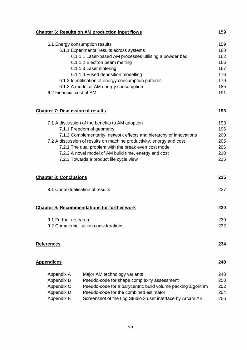
Chapter 6: Results on AM production input flows 159

6.1 Energy consumption results 159

6.1.1 Experimental results across systems 160

6.1.1.1 Laser-based AM processes utilising a powder bed 162

6.1.1.2 Electron beam melting 166

6.1.1.3 Laser sintering 167

6.1.1.4 Fused deposition modelling 176

6.1.2 Identification of energy consumption patterns 179

6.1.3 A model of AM energy consumption 185

6.2 Financial cost of AM 191

Chapter 7: Discussion of results 193

7.1 A discussion of the benefits to AM adoption 193

7.1.1 Freedom of geometry 196

7.1.2 Complementarity, network effects and hierarchy of innovations 200

7.2 A discussion of results on machine productivity, energy and cost 205

7.2.1 The dual problem with the break even cost model 206

7.2.2 A novel model of AM build time, energy and cost 210

7.2.3 Towards a product life cycle view 215

Chapter 8: Conclusions 225

8.1 Contextualisation of results 227

Chapter 9: Recommendations for further work 230

9.1 Further research 230

9.2 Commercialisation considerations 232

References 234

Appendices 248

Appendix A Major AM technology variants 248

Appendix B Pseudo-code for shape complexity assessment 250

Appendix C Pseudo-code for a barycentric build volume packing algorithm 252

Appendix D Pseudo-code for the combined estimator 254

Appendix E Screenshot of the Log Studio 3 user interface by Arcam AB 256

1

Chapter 1: Introduction

Additive Manufacturing (AM) techniques were invented to address problems that have

troubled the makers of things throughout human history. The simple intuition behind

AM is that the technology gives the user the ability to effectively „print‟ objects from

three dimensional (3D) data. In theory, this allows anyone who possesses 3D design

data or is able to create these data to manufacture the objects desired.

This concept is easily understood and has captivated the imagination of many

engineers, scientists and journalists – often leading to speculation on the impact that

such technology might have on the manufacturing environment and wider society. It

may well be that AM is a significant rung on humanity‟s ladder towards ultimate future

manufacturing techniques allowing individuals to create items, involving little or no

manual skill, few resources and minimal technological constraints. After all, in the

words of Gershenfeld (2005), the “world of tomorrow can be glimpsed in tools

available today”.

AM is a relatively recent manufacturing approach, based on technologies originally

intended for the automated production of prototypes. These Rapid Prototyping (RP)

systems were developed in the 1980s and 1990s (Levy et al., 2003). A suitable

definition encapsulating the nature of AM technology is provided by Wohlers (2007):

“Unlike machining processes, which are subtractive in nature,

additive systems join together liquid, powder, or sheet materials to

form parts. Parts that may be difficult or even impossible to fabricate

by any other method can be produced by additive systems. Based on

thin, horizontal cross sections taken from a 3D computer model, they

2

produce plastic, metal, ceramic, or composite parts, layer upon

layer.”

In an effort to establish a set of standards fundamental to AM technology and practise,

the ASTM (2012) define AM processes as being capable of “joining materials to make

objects from 3D model data, usually layer upon layer, as opposed to subtractive

manufacturing methodologies. Synonyms [include]: additive fabrication, additive

processes, additive techniques, additive layer manufacturing, layer manufacturing and

freeform fabrication”.

Both definitions express that AM constitutes an innovation at the centre of

manufacturing technology, used directly in the creation of tangible products or product

features. The breadth of the spectrum of available AM technology variants, in terms of

processes and materials, is also indicated in these definitions. As this thesis

documents, the implications of the additive mode of production are significant and, if

adopted, may introduce previously unknown economic aspects into manufacturing.

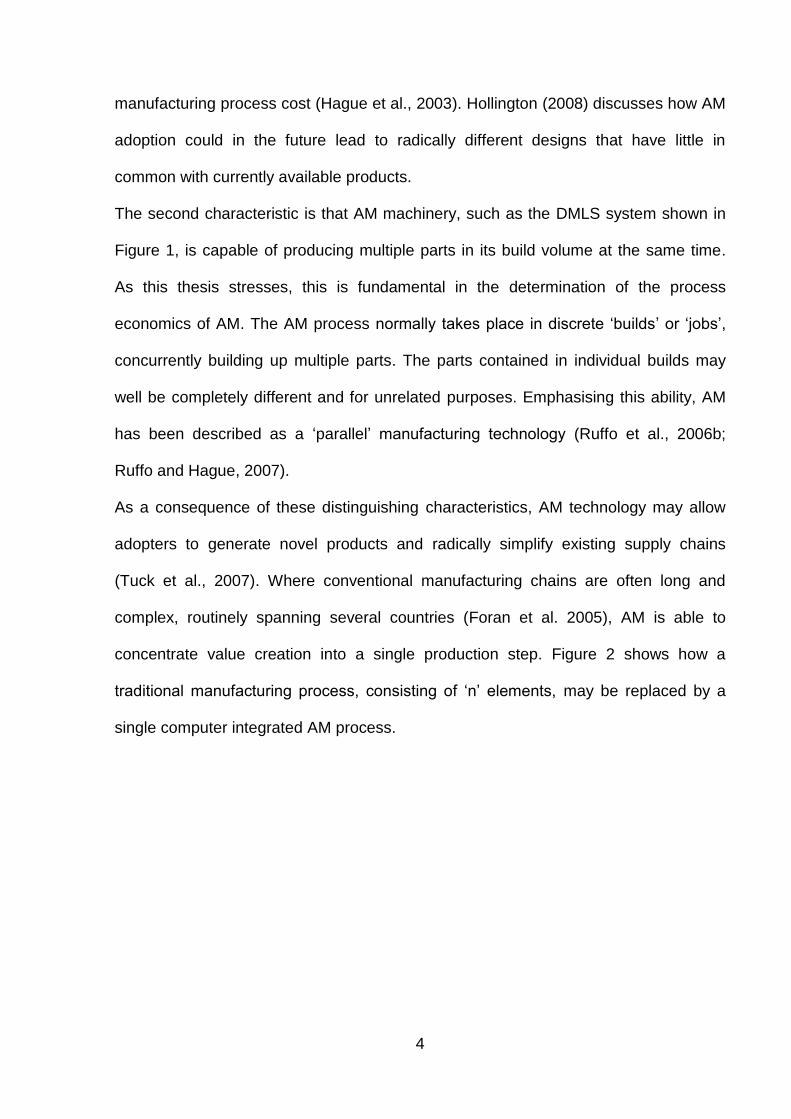
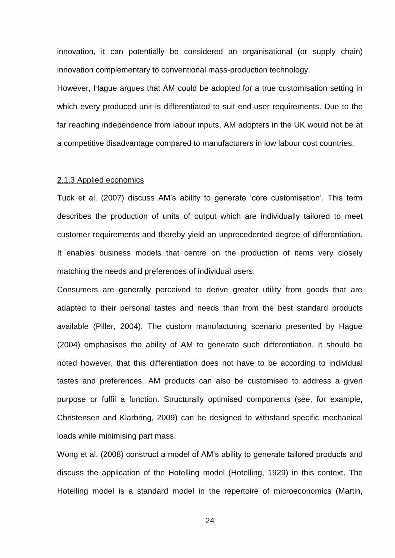
As an example for AM machinery commercially available today, Figure 1 shows the

EOSINT M270 direct metal laser sintering (DMLS) system by equipment manufacturer

EOS GmbH (2010). As for most additive technology variants, the construction of parts

on this machine takes place in an enclosed internal build volume. In this inner

workspace, parts are built up layer-by-layer. An immediate implication is that the size

of the build chamber limits the physical dimensions of AM products. In most AM

variants, the progress of the additive build can be watched through a window in the

build chamber door, which can be seen on the left side of the system shown in Figure

1. For control and data exchange, many AM systems incorporate a personal computer

3

(PC). The input and output devices belonging to this PC are visible on the right hand

side of the system.

Figure 1: An example for an additive manufacturing system (EOSINT M270)

Image source: EOS GmbH (2010)

This thesis is based on the fundamental assumption that two characteristics shape the

process economics of AM, thereby setting AM apart from the existing conventional

manufacturing approaches, such as injection moulding, machining and casting

processes.

The first characteristic is that AM is able to very effectively create complex product

geometry and component shapes. Mapping out the consequences of AM‟s freedom in

terms of product design, Hague et al. (2003) suggest that in AM, added design

complexity may be available at no extra manufacturing cost. The presence of such

„freedom of design‟ would allow AM adopters to realise almost any design they can

envision. Supposing that optimised designs will also be very complex, it is highly

relevant for production economics that product complexity may be decoupled from

4

manufacturing process cost (Hague et al., 2003). Hollington (2008) discusses how AM

adoption could in the future lead to radically different designs that have little in

common with currently available products.

The second characteristic is that AM machinery, such as the DMLS system shown in

Figure 1, is capable of producing multiple parts in its build volume at the same time.

As this thesis stresses, this is fundamental in the determination of the process

economics of AM. The AM process normally takes place in discrete „builds‟ or „jobs‟,

concurrently building up multiple parts. The parts contained in individual builds may

well be completely different and for unrelated purposes. Emphasising this ability, AM

has been described as a „parallel‟ manufacturing technology (Ruffo et al., 2006b;

Ruffo and Hague, 2007).

As a consequence of these distinguishing characteristics, AM technology may allow

adopters to generate novel products and radically simplify existing supply chains

(Tuck et al., 2007). Where conventional manufacturing chains are often long and

complex, routinely spanning several countries (Foran et al. 2005), AM is able to

concentrate value creation into a single production step. Figure 2 shows how a

traditional manufacturing process, consisting of „n‟ elements, may be replaced by a

single computer integrated AM process.

5

Figure 2:Length of production chain of AM compared to other processes

Image source: own work

These aspects make AM an interesting addition to the available spectrum of

technology in the current manufacturing landscape. Nevertheless, AM users, machine

developers and researchers are interested in going beyond this and finding out what

the underlying economic and commercial implications of the adoption of AM are.

Borrowing from the methodology used in the study of technological diffusion, this

thesis operates from the premise that AM‟s future impact will be shaped by two

aspects: the benefits and the costs arising from its use.

The reduction of energy consumption associated with durable goods manufacturing

and usage may be a further benefit of the adoption of AM technology. As outlined in

the feasibility study of the Atkins project at Loughborough University (ATKINS

feasibility study, 2008), to which the research performed for this thesis contributed,

energy savings resulting from technology adoption decisions may effectively occur on

two levels. Firstly, process choice is likely to affect the energy consumed directly

during the manufacturing process. Secondly, the design possibilities connected to

process selection may also affect the energy consumed during other, earlier or later,

6

stages in the product life cycle. It would be possible, for example, that the freedom of

design afforded by AM enables more lightweight designs. These would require less

raw material and hence less energy consumption for raw material production. Such

lightweight designs may also significantly reduce use-phase energy consumption, for

example, in transport applications (Helms and Lambrecht, 2006).

Researchers argue that the limitation of carbon emissions associated with energy

consumption is urgent (Westkämper et al., 2000; Jovane et al., 2008). According to

data from the World Resources Institute, industrial energy consumption, industrial

processes and transportation contributed 33.3 % of world greenhouse gas emissions

in 2005 (Herzog, 2009). Predictions suggest, however, that the energy consumption

occurring in the manufacturing sector will grow faster than in any other sector until

2050 (Taylor, 2008).

1.1 Available additive manufacturing technology

Comparing AM to conventional manufacturing processes, two main advantages have

been identified by Tuck et al. (2008): firstly, AM may enable production without many

of the constraints on part geometry that apply to other techniques, as embodied by the

concept of freedom of geometry. This may lead to products featuring a complex

geometry and to the integration of multiple functions into single components.

Secondly, AM allows the manufacture of highly customised products in small

quantities at a relatively low cost.

As argued by Tuck et al. (2007), the adoption of AM is also likely to enable new

business models. These feature the production of customised or high value products,

very wide product lines, dematerialisation of supply chains, distributed manufacturing

operations, more frequent product improvements and process innovations.

7

At the current state of technology however, the routine application of AM is still

hampered by a number of limiting factors (Ruffo and Hague, 2007):

limited material suitability,

diminished process productivity,

problems with dimensional accuracy,

poor surface finish,

repeatability issues,

uncompetitive production cost at medium and large volumes.

In response to the technology‟s current shortcomings in terms of dimensional

accuracy and surface finish, metallic AM products are often subject to ancillary post-

processing operations. Some AM processes are therefore referred to as „near net

shape‟ processes. Routine post processing techniques include light finish machining

(Cormier et al., 2004) and shot blasting (Mazzioli et al., 2009).

A number of AM technology variants are available in the marketplace. Appendix A

presents a summary of major AM technology types in tabular form with some

fundamental information on each.

8

1.2 Investigating „economics‟ and including energy consumption

This thesis constitutes a treatment of „the economics of AM‟. Therefore, it is necessary

to define clearly what is meant by the term „economics‟ and why this label has been

chosen. Vickers (2003) describes economics as „the science of incentives‟. As such,

the economics of a particular subject or activity are determined by the relationship

between the costs and benefits associated – the difference of both manifesting itself in

an incentive (or disincentive) for participants. Therefore, the underlying strategy of this

thesis is to systematically explore the benefits and costs associated with AM

technology adoption and usage.

In the economic theory of the firm, actors are usually considered to be businesses that

maximise profits. Traditionally, profits are seen as the single incentive and purpose to

the private enterprise. For this analysis, it is helpful to view firm profits as the outcome

of the relationship between two variables: the revenue obtained from some business

activity, for example selling Q units of a product, and the costs associated with the

sale of these Q units.

In a simple static model, this can be illustrated graphically as shown in Figure 3 (see,

for example, Else and Curwen, 1990). In the diagram, the horizontal axis describes

the quantity Q of some good, the vertical axis shows a price P. The straight line MR

shows the revenue (or benefit) a company can obtain from the sale of each marginal

(or „extra‟) unit of Q. This line is downward sloping to reflect that the buyers are willing

to buy more units when the price decreases.

9

Figure 3: Firm behaviour as the interaction of cost and benefit

Image source: adapted from Else and Curwen, 1990

The curve MC describes the cost to the seller of each marginal unit sold. The „U‟

shaped curve shows that initially, where product volumes are small, the cost of each

extra unit decreases. This could, using the example of tooled manufacturing

processes, be due to the sunk costs of tooling which is incurred for the production of

the first unit but not for the subsequent units. As quantity expands, according to the

theory of the firm, MC first bottoms out and then gradually starts sloping upwards. The

reason for this lies in extra costs associated with large quantities, for example, due to

increasing administration overheads.

In this model, a profit maximizing firm will set quantity Q1 such that the revenue for

each extra unit balances the cost of this unit (MR = MC), implying that no additional

profits can be made from expanding output quantity any further. In the static model

shown in Figure 3, the shaded area A reflects the profit that the firm makes from

setting optimal quantity Q1.

10

The purpose of this example is to introduce the concept of marginal cost and to

illustrate that the economics of industries and markets are determined through the

interplay of benefits and costs, as suggested by Vickers (2003).

The logic of exploiting all available profits also applies to the decisions concerning the

uptake of new technologies. Thus, the diffusion of innovations and the resulting

technological impact is equally shaped by costs and benefits (Stoneman, 2002).

Moreover, this suggests that knowledge of the costs and benefits associated with a

new technology can be used to form rational opinions about its future development.

This thesis introduces a further layer of economic analysis by including the energy

consumption aspect in this consideration of process economics. This means that

energy consumption is effectively treated as a secondary type of cost. The rationale

for doing this is as follows: the consequences of carbon emissions resulting from

manufacturing activity (i.e. pollution) arise to society as a whole, as „social costs‟. The

fundamental characteristic of these costs it that they are not exclusively borne by

those responsible for the pollution. For electricity-driven manufacturing technologies,

such as AM, the total social costs are expected to correlate heavily with energy

consumption. Therefore, an understanding of the energy consumption of AM is critical

for an appraisal of the social costs attached to the technology‟s usage.

Normally, social costs are not assumed to be part of the rational choices made by

profit maximising technology users. However, due to the increasing importance of

these issues, it appears justified to include the energy consumed by the AM process in

an analysis of economic aspects.

11

1.3 Aims and objectives of this PhD thesis

In the wider context of applied production economics, this thesis promotes the

understanding of the origin of future improvements in manufacturing productivity.

According to Krugman (1998), such improvements are facilitated primarily through

technological progress and automation. The evolution and diffusion of information

technology has led to significant technological change (Schaller, 1997). It appears that

the most significant innovations generate technology diffusion across different sectors

(Stoneman, 2002). In this sense, AM could be seen as a technological „spill over‟ from

the IT sector into general manufacturing.

Commenting on the ethical dimension of researching new technologies, Sahal (1985)

suggests that there is an obligation to maximise the ex-ante understanding of

promising innovations: to “put the matter in a nutshell, we need unequivocal ways of

measuring technology so as to create public awareness of innovations and to ensure

consumer sovereignty”.

This research aims to address a number of specific research objectives, designed to

cultivate an understanding of central aspects of the economics of AM. Based on the

view of economics as the science of incentives, as suggested by Vickers (2003), this

research systematically measures the benefits and costs of AM, including the process

energy consumption representing the social cost aspect. Three primary research

objectives related to the economics of AM are pursued in this thesis:

12

I. Regarding the monetary cost of AM, it has been argued that extra complexity

may be available without cost (Hague et al., 2003). Treating process energy

consumption as a major determinant of the associated social costs, it is

important to address the question of whether increasing the complexity of the

shape of a product results in increased process energy consumption in AM.

II. As this thesis argues, reliable empirical data and summary metrics on build

speed, energy consumption and cost for major additive platforms are required.

This is mainly due to problems in the existing analyses arising from the fact that

they are specified with unused machine capacity. This is likely to result in

inefficient technology usage. Therefore, it is an objective of this research to

generate a set of machine productivity, energy consumption and cost results

that reflect technically efficient machine operation.

III. To develop a valid technique for the combined ex ante estimation of build time,

energy consumption and cost. A novel tool is devised to handle the multi-part

and multi-product case typically (and exclusively) found in AM applications.

Analogous to research objective II, AM‟s ability to fill builds with different and

potentially unrelated parts causes problems in the estimation of build time,

energy consumption and cost.

A subordinate objective of this thesis is to demonstrate that where the creation of part

geometry is concentrated into a single production step (illustrated in Figure 2, page 5),

the measurement of input flows used to transform raw material into finished (or nearly

13

finished) components is greatly simplified. Therefore, next to impacting production

cost and energy consumption, the adoption of AM may promote accountability in

terms of manufacturing cost and process energy consumption. This aspect is of

growing importance to consumer sovereignty, as data on the environmental footprint

of products are increasingly moving into the consumer‟s consciousness.

Summarising the presented research objectives in one sentence, this thesis

contributes to the understanding of the economics of AM through an analysis of the

effect of AM‟s parallel nature on economic and environmental performance

measurement and AM‟s ability to efficiently create product complexity. If this analysis

is successful, it may help avoid erroneous conclusions about the usefulness of digitally

integrated manufacturing technologies. Reflecting on such errors, Neil Gershenfeld

(2007) comments the following:

“I‟d like to argue that it‟s done, we won. We‟ve had a digital revolution

but we don‟t need to keep having it. And I‟d like […] to look what

comes after the digital revolution.”

14

1.4 Structure of this thesis

This thesis is structured with a conventional sequence of chapters on existing

literature, used methodology, obtained results and discussion of results. This orthodox

approach is chosen due to the strong interdisciplinary flavour of this work, building on

theory from manufacturing engineering, production economics, technology adoption,

industrial ecology and shape complexity theory. Where numerical and optimisation

problems are encountered, algorithms are implemented to overcome these. Therefore,

this work also includes an element of algorithm design, specifically in the area of build

volume packing, complexity measurement and build time, energy consumption and

cost estimation.

To aid reader orientation, this thesis attempts to keep the order in which the various

fields of literature are treated identical throughout the chapters. To further improve

clarity, the chapters have consistently been subdivided into sections separately

discussing the topics associated with benefits and the costs (including energy usage)

of AM technology usage.

For added structure, the results are discussed separately in three chapters: the

benefits of AM (Chapter 4), results on machine productivity (Chapter 5), and results on

production input utilisation (Chapter 6).

In the discussion chapter, this thesis departs from the fixed order of treatment of the

individual areas of literature and discusses the material along five identified discussion

themes. The final two chapters draw conclusions and present possibilities for further

work. Figure 4 graphically summarises the structure of this thesis.

15

Figure 4: Overview of thesis structure

Image source: own work

1.5 Published work

During the initial planning phase of the doctoral project leading to this thesis, a

publication strategy was devised. Due to the interdisciplinary nature of this work, it

was decided that the performed research should receive peer review where ever

possible; this approach resulted in five peer reviewed publications.

The first peer-reviewed conference contribution was made to the 2010 Solid Freeform

Fabrication (SFF) Symposium. It introduces a common methodology for the

16

measurement of energy inputs to metallic AM processes and is titled “A comparative

study of metallic additive manufacturing power consumption” (Baumers et al., 2010).

An empirical measurement of realised levels of product complexity found in AM

products performed by Baumers et al. (2011a) contributes to the analysis of the

benefits arising from AM technology usage.

A submission to the SFF Symposium in 2011 expands the findings of Baumers et al.

(2010) to a wide range of polymeric and metallic platforms and adds a further layer of

analysis on the effects of capacity utilisation. It is titled “Energy inputs to additive

manufacturing: does capacity utilization matter” (Baumers et al., 2011b).

The following journal paper surveys in detail the energy consumption of two competing

commercial laser sintering (LS) systems and is published in the Institution of

Mechanical Engineers Part B: Journal of Engineering manufacture in 2011. It is titled

“Sustainability of additive manufacturing: measuring the energy consumption of the

laser sintering process” (Baumers et al., 2011c).

The developed energy consumption measurement methodology is combined with a

novel cost model for AM in a following journal article. It has been accepted for

publication in 2012 by the Journal of Industrial Ecology. This article is titled

“Transparency built-in: energy consumption and cost estimation for additive

manufacturing” (Baumers et al., forthcoming).

A further article that has been prepared in the process of this PhD project deals with

AM energy consumption. It analyses the total energy requirements during the

production of titanium-alloy parts using the electron beam melting (EBM) process. The

planned title for this paper is “Energy inputs to the production of titanium parts:

additive manufacturing versus conventional milling”. It is undergoing additional

preparation.

17

Chapter 2: Literature review

The interdisciplinary character of this project requires the incorporation of ideas and

concepts from a wide range of areas. While applied economics forms the theoretical

basis, this thesis draws on literature studying manufacturing engineering,

technological change, organisational strategy and complexity theory. This review

chapter attempts to provide an accessible and coherent account of the concepts

contained in this eclectic combination of literature.

Initially, a broad distinction between two types of literature is made: a background

theory section concentrates on the treatment of literature on general concepts helpful

in the analysis of the issues at hand. The following sections on focal theory deal with

the areas of literature needed to address the research objectives. Section 2.4

summarises the identified gaps in the literature and how they relate to the research

objectives. The surveyed focal theory includes the following topics: shape complexity,

design for manufacturability, AM build time estimation, energy consumption,

production cost and build volume utilisation.

2.1 A review of background theory

In this review of background material, section 2.1.1 begins by discussing some items

relevant to the economics of AM in the field of futurologist literature. Futurologist

studies explore how the innovation of AM may in the future impact people‟s everyday

lives and the economy.

Following this, Section 2.1.2 provides an account of the AM related literature

describing the present situation in the manufacturing sector in the UK, with an

emphasis on global differences in labour costs. Section 2.1.3 offers a classification of

AM technology in the framework of applied economics. This classification is further

18

elaborated in section 2.1.4, where empirical observations from the additive industry

are put into the context of durable goods theory. Section 2.1.5 presents a brief

discussion of the economics of technology diffusion and its applicability to AM. The

appropriate organisational changes accompanying the adoption of AM are discussed

in section 2.1.6.

2.1.1 Additive techniques in the futurologist literature

Futurologist methods, which can be heavily speculative, have been employed to make

statements on the economic implications of AM on manufacturing activity. This work

has received attention in the broader public and perhaps forms a good starting point

for this literature review. It also provides a colourful overview of the broad types of

ideas that are discussed in the context of future AM usage.

According to Schnaars (1989), futurologist predictions of the impact of technologies

are “one of the most difficult kinds of forecast to make accurately. There are so many

unknowns, and so many possible outcomes, that errors appear everywhere”.

Adhering to the futurologist convention of presenting a range of conceivable scenarios

for technology usage, Neef et al. (2005) suggest three different alternatives for the

diffusion of AM technology. The most radical scenario discussed by Neef et al. is the

utopian „home-fabber‟ scenario which was originally proposed by Burns (1993). This

scenario predicted that the most advanced households could by 2008 incorporate a

special room with additive machinery. This „fabricator room‟ would supposedly be

used by the members of the household to produce durable goods for their own needs.

In a similarly utopian vision, Bergmann (2004) claims that the arrival of AM technology

will allow individuals to bypass the markets for many products and goods. This would

be done by implementing a form of high-technology subsistence production, possibly

19

in collectives. Bergmann argues that through the adoption of novel manufacturing

approaches the „prosumer‟ (a portmanteau of „producer‟ and „consumer‟) will emerge.

The second scenario proposed by Neef et al. is labelled the „copy shop‟ scenario, or

alternatively the „Kinko‟ scenario, after a chain of outlets offering copy and print

services. Neef et al. suggest that individuals will submit the designs of products they

need, in the form of 3D data, to local additive production facilities. Like the predictions

of the type expressed by Burns and Bergmann, this approach also bypasses the

manufacturing industry. Therefore, widespread AM technology adoption of this kind

would constitute a fundamental shift away from the present order in which durable

goods are almost exclusively produced by specialist firms in a commercial

manufacturing sector.

Schnaars (1989) advises caution when dealing with such technological forecasts.

Referring to the poor track record of claims that individual new technologies will

change everyday lives, Schnaars contends that “[the] most prominent reason why

technological forecasts have failed is that the people who made them have been

seduced by technological wonder. […] Most of those forecasts fail because the

forecasters fall in love with the technology […]”. Investigating such errors, Avison and

Nettler (1976) conclude that “a conservative and pessimistic attitude tends to

illuminate the crystal ball, while a liberal and optimistic attitude tends to darken it”.

Interestingly, developments in the present (in 2012) appear to have overtaken the

„Kinko‟ scenario. Web-based service providers, such as Shapeways (2011) and

Fabberhouse (2011), offer very affordable AM services to anyone capable of providing

the necessary 3D data, including private end-users. Moreover, Kinko‟s no longer

exists as an independent business (FedEx, 2008).

20

The third, and more conservative, scenario proposed by Neef et al. is the use of AM

systems in the commercial manufacturing industry. This scenario does not include an

utopian vision of the end of the division line between producers and consumers.

Nevertheless, this scenario assumes that AM has the potential to technologically and

economically greatly advance manufacturing practice and also product design.

In their discussion of the commercial application of new manufacturing technology,

Friebe and Ramge (2008) present an assessment of the potential impact of AM,

based on the perceived trends towards individualisation, peer networks and greatly

reduced transaction costs enabled by information technology (IT).

Friebe and Ramge suggest that AM forms an ideal technology to serve markets

demanding highly individualised but affordable goods in low volumes. The authors

explain how AM may serve what they refer to as a „long tail‟ demand structure.

According to Friebe and Ramge this concept was returned to the public attention by

Anderson (2006), who observed a distinct pattern in a survey of sales data provided

by an online vendor of music, videos and books: large cumulative sales numbers are

achieved with items that only appeal to a very narrow group of customers and sell

infrequently. In consequence a distribution of sales frequency with a long tail can be

observed, as shown in Figure 5.

21

Figure 5: Long tail distribution of sales

Image source: adapted from Friebe and Ramge, 2008

According to Friebe and Ramge, the move towards more individualised consumption

patterns has caused the observed change. It is claimed that in industries in which this

development has taken place many more low volume items are now sold. The

increase in sales occurs at the expense of traditional high volume products.

2.1.2 Current developments in manufacturing and the role of AM

A paper by Hague (2004) offers an overview of the broad alternatives in the future of

UK manufacturing. Three „viable future UK manufacturing models‟ are identified and

discussed in the light of a potential large-scale adoption of AM.

The first alternative focuses on the traditional method of mass production, relying on

capital inputs and labour to create economies of scale and realise high levels of

productivity. However, this mode of production is limited to industries in which

accepted, standardised products with robust designs are prevalent (Utterback, 1993).

Further, traditional mass production generates narrow product lines and draws heavily

0

22

on unskilled labour inputs (Milgrom and Roberts, 1995). As a result of the emphasis

on unskilled labour inputs in the mass production approach, this style of production

has largely shifted away from economies where labour costs are high, such as in the

UK.

In an effort to stimulate the manufacturing sector in the UK, manufacturing process

innovations compatible with high labour cost environments are being sought. Due to

the ability of AM to reduce unskilled and skilled labour inputs to production, AM is

viewed as a viable option in economies with comparatively high wage levels in

manufacturing (Hague, 2004).

In direct competition with conventional mass production, however, AM faces the

disadvantage of not being able to offer the economies of scale available to

conventional manufacturing processes. As suggested by Ruffo et al. (2006b), these

economies of scale can result from the use of dedicated tooling in conventional

manufacturing. An example for this are injection moulding processes in which

production volumes are high and designs are compatible with conventional mass

production methods.

The second alternative proposed by Hague (2004) describes a situation in which UK

manufacturing concentrates on the production of sophisticated, high value products in

relatively low volumes. Here, companies generate technologically advanced products

through extensive research and development (R&D) expenditure, effectively adding

value to their products in the design and engineering stages.

To assess the viability of this scenario it is instructive to assess the levels of business

R&D spending in high and low labour cost countries. Following Patel and Pavitt

(1995), most R&D expenditure undertaken in the private sector is either for close to

market applied research or direct spending associated with the development of

23

marketable products. Therefore, business R&D spending can be interpreted as a

prerequisite for the high value engineering model and can thus be used as a basic

indicator of the UK‟s competitive standing in high value added manufacturing.

However, business R&D spending data for selected countries (OECD, 2007;

Pottelsberghe, 2008) show that this type of spending may not be small in low wage

economies, such as China, at least when measured as a share of gross domestic

product (GDP). Moreover, the business R&D spending has exhibited a downward

trend in the UK from 1995 to 2006 (OECD, 2007).

Hague acknowledges that emerging economies such as China, which are at the

receiving end of UK manufacturing outsourcing activity, now have a financial system in

place supporting the private sector. Pottelsberghe (2008) comments that Chinese

business funded R&D intensity is now higher than that of the European Union (0.82 %,

median value). Hague concludes that this scenario, which may involve the extensive

adoption of AM to create differentiated and complex products, would be hazardous for

UK manufacturing.

The third alternative scenario discussed by Hague is labelled the „mass-customisation‟

scenario. This name proves somewhat misleading: the approach known as mass-

customisation is technically a form of modularisation, delaying the differentiation of the

final product to the latest possible point in the supply chain (Tuck et al., 2007). This

creates quasi-personalised product characteristics through customised combinations

of pre-fabricated (and conventionally mass produced) components. However, the

scale economies available and the necessity of labour inputs therefore make the

mass-customisation approach prone to the same outsourcing phenomena

experienced by conventional mass production in the UK (Hague, 2004). Because

mass-customisation is not based on an underlying manufacturing technology

24

innovation, it can potentially be considered an organisational (or supply chain)

innovation complementary to conventional mass-production technology.

However, Hague argues that AM could be adopted for a true customisation setting in

which every produced unit is differentiated to suit end-user requirements. Due to the

far reaching independence from labour inputs, AM adopters in the UK would not be at

a competitive disadvantage compared to manufacturers in low labour cost countries.

2.1.3 Applied economics

Tuck et al. (2007) discuss AM‟s ability to generate „core customisation‟. This term

describes the production of units of output which are individually tailored to meet

customer requirements and thereby yield an unprecedented degree of differentiation.

It enables business models that centre on the production of items very closely

matching the needs and preferences of individual users.

Consumers are generally perceived to derive greater utility from goods that are

adapted to their personal tastes and needs than from the best standard products

available (Piller, 2004). The custom manufacturing scenario presented by Hague

(2004) emphasises the ability of AM to generate such differentiation. It should be

noted however, that this differentiation does not have to be according to individual

tastes and preferences. AM products can also be customised to address a given

purpose or fulfil a function. Structurally optimised components (see, for example,

Christensen and Klarbring, 2009) can be designed to withstand specific mechanical

loads while minimising part mass.

Wong et al. (2008) construct a model of AM‟s ability to generate tailored products and

discuss the application of the Hotelling model (Hotelling, 1929) in this context. The

Hotelling model is a standard model in the repertoire of microeconomics (Martin,

25

2001). It is also relevant for the treatment of the impact of horizontal differentiation on

technological diffusion (Stoneman, 2002).

Wong et al. (2008) use their model to benchmark an AM based production approach

against two other approaches. Firstly, it is compared to a conventional make-to-stock

mass production approach, as introduced in the previous section 2.1.2. Secondly, it is

compared to a delayed differentiation route. This is especially interesting as the

delayed differentiation route corresponds to what Tuck et al. (2007) describe as

„modularisation‟: the configuration of the final product from standardised modules is

delayed as long as possible. Wong et al. refer to AM as „custom manufacturing‟ and

alternatively „ultimate customisation‟.

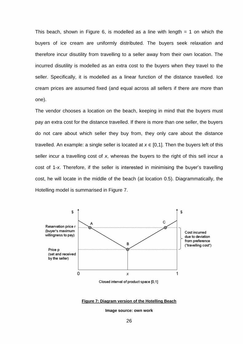
The Hotelling model was developed in 1929 to illustrate spatial product differentiation,

modelling the impact of a seller‟s geographic location on business. This model is

normally explained using the example of one or more ice-cream vendors on a beach

(Cabral, 2000; Wong et al., 2008).

Figure 6: The Hotelling Beach, adapted from Wong, et al. (2008)

Image source: own work, image from http://www.nwmangum.com/BVIPanos/index.html

26

This beach, shown in Figure 6, is modelled as a line with length = 1 on which the

buyers of ice cream are uniformly distributed. The buyers seek relaxation and

therefore incur disutility from travelling to a seller away from their own location. The

incurred disutility is modelled as an extra cost to the buyers when they travel to the

seller. Specifically, it is modelled as a linear function of the distance travelled. Ice

cream prices are assumed fixed (and equal across all sellers if there are more than

one).

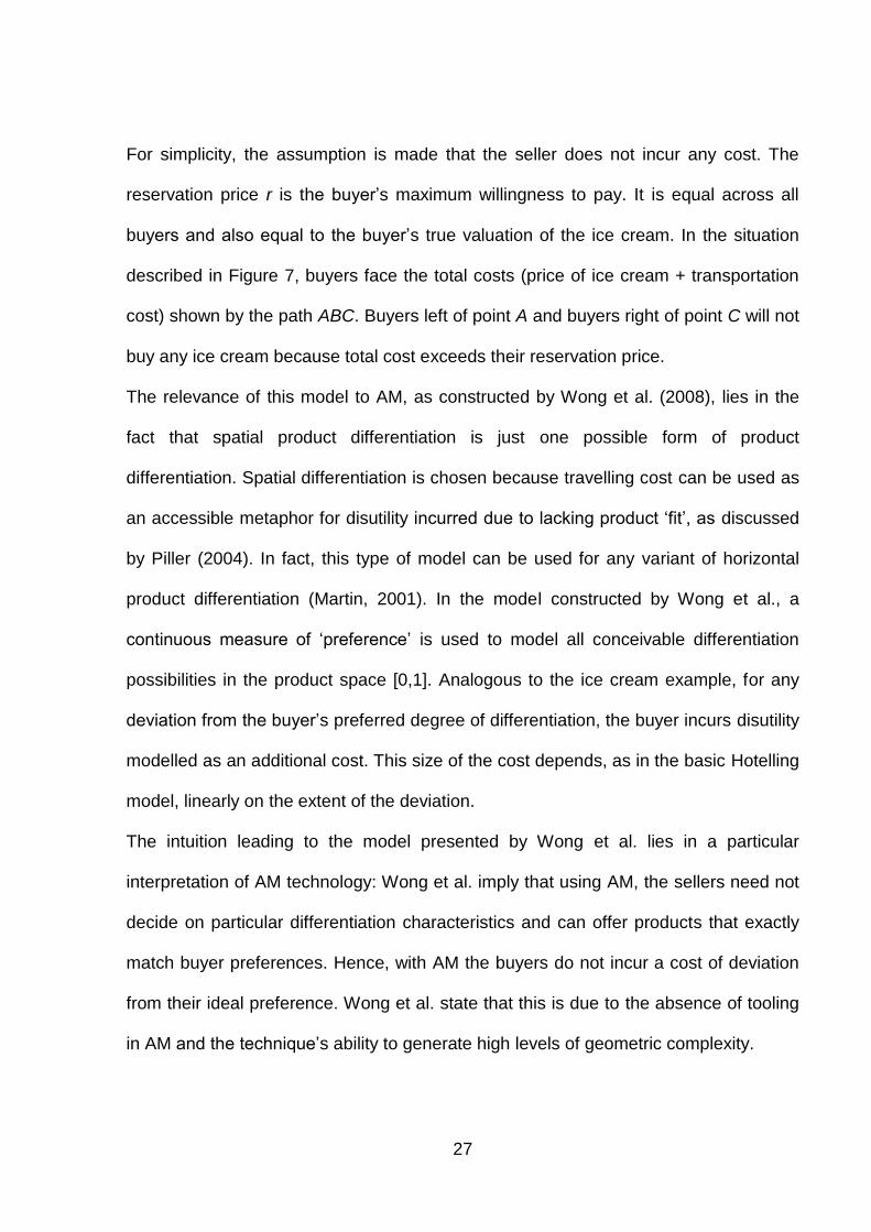
The vendor chooses a location on the beach, keeping in mind that the buyers must

pay an extra cost for the distance travelled. If there is more than one seller, the buyers

do not care about which seller they buy from, they only care about the distance

travelled. An example: a single seller is located at x ∈ [0,1]. Then the buyers left of this

seller incur a travelling cost of x, whereas the buyers to the right of this sell incur a

cost of 1-x. Therefore, if the seller is interested in minimising the buyer‟s travelling

cost, he will locate in the middle of the beach (at location 0.5). Diagrammatically, the

Hotelling model is summarised in Figure 7.

Figure 7: Diagram version of the Hotelling Beach

Image source: own work

27

For simplicity, the assumption is made that the seller does not incur any cost. The

reservation price r is the buyer‟s maximum willingness to pay. It is equal across all

buyers and also equal to the buyer‟s true valuation of the ice cream. In the situation

described in Figure 7, buyers face the total costs (price of ice cream + transportation

cost) shown by the path ABC. Buyers left of point A and buyers right of point C will not

buy any ice cream because total cost exceeds their reservation price.

The relevance of this model to AM, as constructed by Wong et al. (2008), lies in the

fact that spatial product differentiation is just one possible form of product

differentiation. Spatial differentiation is chosen because travelling cost can be used as

an accessible metaphor for disutility incurred due to lacking product „fit‟, as discussed

by Piller (2004). In fact, this type of model can be used for any variant of horizontal

product differentiation (Martin, 2001). In the model constructed by Wong et al., a

continuous measure of „preference‟ is used to model all conceivable differentiation

possibilities in the product space [0,1]. Analogous to the ice cream example, for any

deviation from the buyer‟s preferred degree of differentiation, the buyer incurs disutility

modelled as an additional cost. This size of the cost depends, as in the basic Hotelling

model, linearly on the extent of the deviation.

The intuition leading to the model presented by Wong et al. lies in a particular

interpretation of AM technology: Wong et al. imply that using AM, the sellers need not

decide on particular differentiation characteristics and can offer products that exactly

match buyer preferences. Hence, with AM the buyers do not incur a cost of deviation

from their ideal preference. Wong et al. state that this is due to the absence of tooling

in AM and the technique‟s ability to generate high levels of geometric complexity.

28

This appraisal of the advantages of AM is repeated in the available literature (Hague

et al., 2004; Wohlers, 2011a; Gebhardt, 2008). It is noteworthy, though, that the model

discussed by Wong et al. is a purely theoretical effort; empirical validation is not

presented.

Next to AM‟s ability to produce differentiation, other factors such as production speed

and stock holding costs are considered. Wong et al. conclude that a number of factors

may impede the commercial viability of AM manufacturing, citing high production cost

(presumably referring to high average cost per unit produced) and long production

lead times.

The assumption of production lead times negatively impacting the competitiveness of

AM contradicts the commonly held belief that AM is an especially „rapid‟ process

(Wohlers, 2011b). The application of the Hotelling model to AM illustrates that the

degree to which product differentiation matters to the buyers affects the overall

prospect of successful AM technology adoption. Following the reasoning presented by

Wong et al., AM is especially applicable where buyers are affected negatively by

deviations from their real preferences. Moreover, if the reservation price is sufficiently

high to make AM production profitable (for example, in the production of prosthetic

implants) AM may have a good chance of being a commercial success. In other areas,

where the penalty for deviating from buyer preferences is not substantial (for example,

in stationery products), the commercialisation prospects of AM may be smaller.

2.1.4 Durable goods theory

An analysis of the relevant background literature for this thesis would be incomplete

without a survey of durable goods theory. This is due to two reasons: firstly, AM

machinery is itself capital equipment constituting a durable good. Secondly, in most

29

cases the products generated by AM will also be durable goods of various kinds, as

discussed by Wohlers (2011a) in the presentation of the current commercial

applications of AM.

Thus, a firm engaged in AM is likely to face durable goods markets both on the input

and on the output side. Waldman (2003) notes that much of the literature on durable

goods treats the purchase of such goods by consumers. It is stressed that the

problems faced by firms selling durable goods as intermediate inputs to other firms (as

AM machinery normally is) are similar.

According to Waldman, the defining feature of a durable good in this context is that the

good does not provide its benefit instantaneously, but instead provides a stream of

services useful to the user over a period of time. This section presents the concepts

introduced by Waldman that are directly applicable to either AM equipment

manufacturers or additively manufactured products.

Initially, the „time inconsistency‟ problem appears relevant to the economics of AM.

Time inconsistency is based on the idea that durable goods sold in the future affect

the future value of the units sold in the present. In the reasoning developed by

Bulow (1982), the buyers of durable goods, such as AM equipment, may not be willing

to pay a particular price set by a single seller in the market (the monopoly price)

because they expect that the seller will reduce his price in the future. Applied to the

determination of the price of capital equipment, such as a LS system, this idea is

trivial.

However, as Waldman points out, the time inconsistency problem affects not only to

pricing strategy, but also any other future actions committed by the seller. These could

be, for example, the commitments to research and development, introduction of norms

and standards, or the introduction of an equipment repurchasing policy. As AM is

30

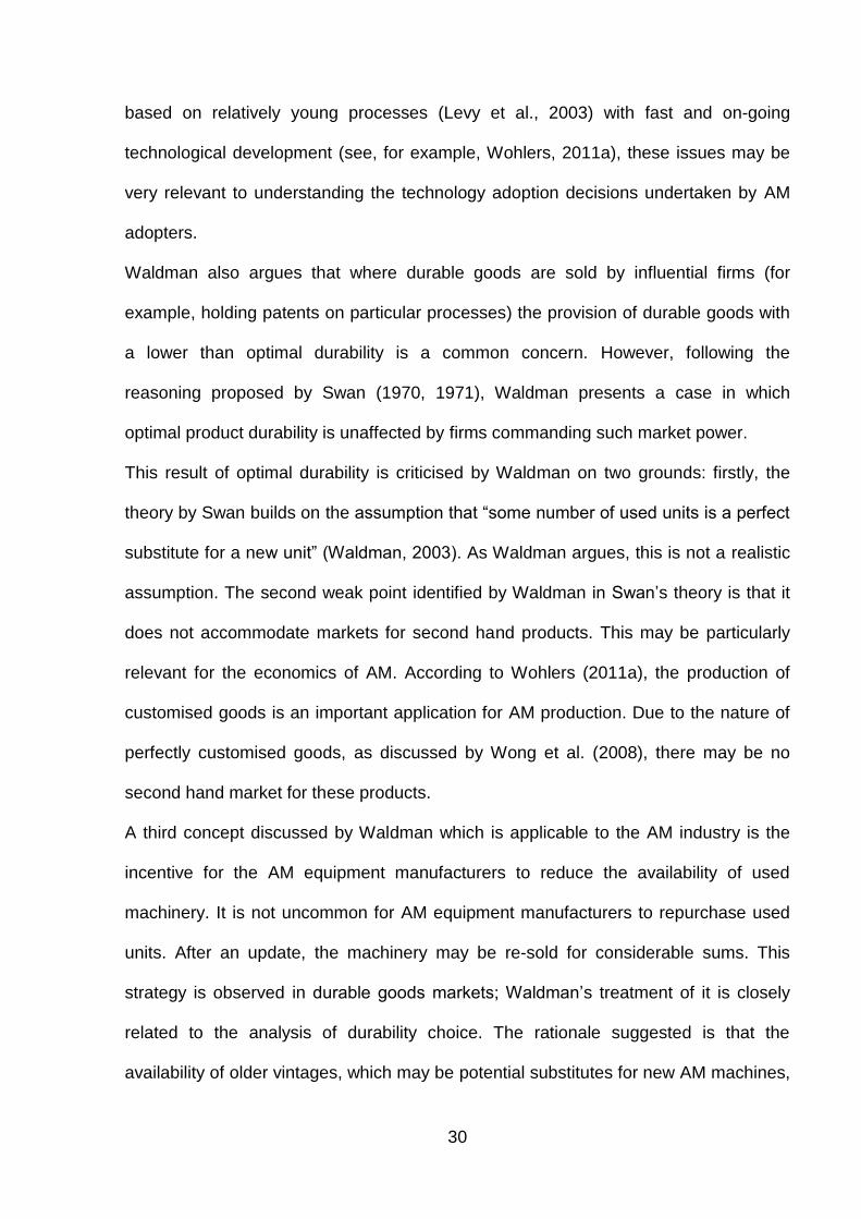
based on relatively young processes (Levy et al., 2003) with fast and on-going

technological development (see, for example, Wohlers, 2011a), these issues may be

very relevant to understanding the technology adoption decisions undertaken by AM

adopters.

Waldman also argues that where durable goods are sold by influential firms (for

example, holding patents on particular processes) the provision of durable goods with

a lower than optimal durability is a common concern. However, following the

reasoning proposed by Swan (1970, 1971), Waldman presents a case in which

optimal product durability is unaffected by firms commanding such market power.

This result of optimal durability is criticised by Waldman on two grounds: firstly, the

theory by Swan builds on the assumption that “some number of used units is a perfect

substitute for a new unit” (Waldman, 2003). As Waldman argues, this is not a realistic

assumption. The second weak point identified by Waldman in Swan‟s theory is that it

does not accommodate markets for second hand products. This may be particularly

relevant for the economics of AM. According to Wohlers (2011a), the production of

customised goods is an important application for AM production. Due to the nature of

perfectly customised goods, as discussed by Wong et al. (2008), there may be no

second hand market for these products.

A third concept discussed by Waldman which is applicable to the AM industry is the

incentive for the AM equipment manufacturers to reduce the availability of used

machinery. It is not uncommon for AM equipment manufacturers to repurchase used

units. After an update, the machinery may be re-sold for considerable sums. This

strategy is observed in durable goods markets; Waldman‟s treatment of it is closely

related to the analysis of durability choice. The rationale suggested is that the

availability of older vintages, which may be potential substitutes for new AM machines,

31

diminishes the prices the manufacturers can charge for new machines. Hence, the AM

equipment manufacturers may be motivated to remove older units from the market,

resulting in higher prices for new units.

A more extreme version of this strategy is a repurchase-and-scrap strategy, which

dictates that older units are bought off the market and scrapped, again motivated by

higher prices achieved for new units. An alternative way to eliminate second-hand

markets is the adoption of a leasing strategy. Here, the suppliers refuse to sell output;

instead, revenue is generated through a strategy of effectively renting out AM

equipment.

A fourth, and final, point raised by Waldman that can be applied to the economics of

AM is the practice of aftermarket monopolisation. Aftermarkets are defined as markets

for goods and services complementary to a durable good, also referred to as

supporting input markets. The documentation made available by NCP Leasing Inc., a

commercial firm specialising in finance for AM systems, offers some insight into the

practises relating to the aftermarkets for additive technology (NCP Leasing Inc., 2010).

For additive technologies, some markets for raw material inputs appear to be

monopolised by the equipment manufacturers. NCP Leasing Inc. notes that “systems

that have a limited range of materials and those for which materials are only available

from the systems manufacturer are likely to suffer compared to more versatile

platforms”. Moreover, in the markets for maintenance services and replacement parts,

both factory maintenance contracts and independent maintenance agreements appear

to exist.

The extent to which the additive equipment manufacturers have power to „lock in‟

technology adopters remains unclear. According to Waldman, the common practise

for sellers to exploit an aftermarket is to first exclude independent firms from this

32

market, effectively monopolising it, and then raising prices to monopoly levels. Buyers

may fail to recognise maintenance cost in their initial technology adoption decision,

particularly if the acquisition of such information is costly (Waldman, 2003).

A final issue raised by NCP Leasing Inc. is that software licensing may affect the

resale values of additive machinery. Proprietary software is needed to operate AM

machinery. However, the software licenses may not be transferrable to second-hand

buyers. The consequence is that used machines can suffer from severely diminished

resale values as the re-licensing of the systems may be at the discretion of the

equipment manufacturer.

2.1.5 Diffusion of innovations

The term „technology‟ has been summarised as the set of presently known

alternatives of converting resources into outputs that are required by the economy

(Griliches, 1987). Therefore, the literature on the diffusion of novel technologies, such

as AM, sees technological change as an information transmission process (Rogers,

2003). Information is depicted as a reduction of uncertainty in situations where

alternative choices are available (Rogers and Kincaid, 1981). Where new technology

is taken up, information is transmitted, reducing uncertainty about the underlying

“cause-effect relationships in problem-solving” (Rogers, 2003).

According to the „Schumpeterian Trilogy‟, named after the Austrian economist Joseph

Schumpeter, the process of technological change consists of three distinct stages

(Stoneman, 1995): in a first stage, ideas are created in the invention process. In a

second stage, these ideas evolve into marketable products and processes; this stage

is referred to as the innovation process. Finally, in a third stage, the new products and

processes spread across potential markets. As Stoneman (1995) notes, there is a

33

consensus that the economic impact of innovations occurs in the phase in which

technologies spread. This stage is labelled the diffusion stage; “in strict terms, the

analysis of diffusion is the analysis of the process by which knowledge is incorporated

into the economy post first incorporation (or innovation)” (Stoneman, 2002).

The literature on diffusion shares a central empirical observation: the diffusion of

innovations over time normally follows an S-shaped curve (Rogers, 2003; Stoneman,

2002; Hall, 2005), as shown in Figure 8.

Figure 8: The S-shaped diffusion curve

Image source: adapted from Stoneman (2002)

In a seminal study on the diffusion innovations, studying the spread of a new type of

corn in different US federal states, Griliches (1957) observes that in state i the extent

of market penetration Pi(t), i.e. the proportion of the total acreage Ni planted with the

new type of corn at time t, exhibits an S-shaped curve when plotted against time.

According to Stoneman (2002), this observation can be generalised in that the uptake

of an innovation begins slowly and accelerates up to an inflection point. After this point

it slows down towards its asymptotic level.

34

It should be noted that the asymptotic level of use, Pi*, is not necessarily unity. In other

words, diffusion does not necessarily reach 100% market penetration. Griliches finds

that the pattern can be represented by the logistic function:

t

ii

iie

PtP

1)(

*

(Eq. 1)

where Pi is the market penetration of the innovation at time t. Pi* is, as defined above,

the asymptotic level of diffusion, the parameter ηi positions the diffusion curve on the

horizontal axis and ϕi is a parameter controlling the diffusion speed.

Among the studies of technological diffusion of manufacturing technology innovation,

a paper of particular interest is an article by Vickery and Northcott (1995), analysing

the diffusion of microelectronics and advanced manufacturing technology across

countries. The investigated sample of advanced manufacturing technology includes

Computer Aided Design / Engineering (CAD/CAE), Numerically Controlled / Computer

Numerical Controlled (NC/CNC), flexible manufacturing systems/centres, pick and

place robots, automated storage retrieval, final inspection systems and factory

computer networking.

As AM may be also classified as an advanced manufacturing technology, the patterns

observed by Vickery and Northcott (1995), as shown in Figure 9, may provide an

indication of how AM will spread.

35

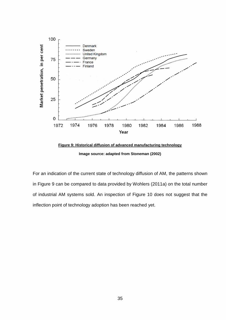
Figure 9: Historical diffusion of advanced manufacturing technology

Image source: adapted from Stoneman (2002)

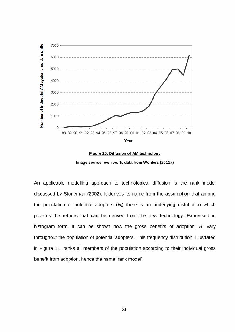
For an indication of the current state of technology diffusion of AM, the patterns shown

in Figure 9 can be compared to data provided by Wohlers (2011a) on the total number

of industrial AM systems sold. An inspection of Figure 10 does not suggest that the

inflection point of technology adoption has been reached yet.

36

Figure 10: Diffusion of AM technology

Image source: own work, data from Wohlers (2011a)

An applicable modelling approach to technological diffusion is the rank model

discussed by Stoneman (2002). It derives its name from the assumption that among

the population of potential adopters (Ni) there is an underlying distribution which

governs the returns that can be derived from the new technology. Expressed in

histogram form, it can be shown how the gross benefits of adoption, B, vary

throughout the population of potential adopters. This frequency distribution, illustrated

in Figure 11, ranks all members of the population according to their individual gross

benefit from adoption, hence the name „rank model‟.

37

Figure 11: Distribution of benefits to technology adoption

Image source: own work

As discussed in the context of economic incentives in section 1.2, potential technology

users will adopt the innovation if the available gross benefit is greater than the

associated cost.

When applied to the distribution of gross benefits illustrated in Figure 11, a proportion

of the population can be defined that will find ownership of the technology profitable

and adopt in time t. For the empirical diffusion path to be mapped out with the

characteristic S-shape (shown in Figure 8, page 33), there are two alternative

possibilities. Firstly, the cost c(t) of the new technology may fall over time, gradually

increasing the share of the population finding the new technology profitable

(movement along the gross benefit distribution in Figure 11). Secondly, the gross

benefits of adoptions might increase as the technology gets „better‟ over time (shifting

the gross benefit distribution to the right).

38

Therefore, the rank model is driven through outside forces. Both cost reduction and

technology improvements are very likely to occur for AM in the future, making a

diffusion path with the commonly observed S-shape likely, should the underlying

distribution pattern of the benefits be compatible with Figure 11.

Considering the variety of factors that might affect the gross and net benefits to

adoption, it appears that the distribution will change over time as the factors affecting it

change. Interactions between the innovation and other technologies (including

organisational innovations) are also very relevant in this context.

In the following, these issues are grouped in four overarching topics, as suggested by

Stoneman (2002): multiple technologies, joint inputs, standards and compatibility, and

general purpose technologies.

2.1.5.1 Interaction between multiple technologies

New technologies introduced to organisations are usually inserted into a system of

already present technologies. Rarely can a new technology be classified a „stand-

alone‟ innovation (Stoneman, 2002). The presence of a combination of newly

introduced and already present technologies can generate returns greater than the

returns to each technology alone. Alternatively, two new technologies can be adopted

alongside each other to exploit such effects. CAD/CAM is an example for such

technologies: Stoneman argues that it is commonly accepted that a combination of

CAD and CAM creates benefits which are greater than the sum of benefits available if

they were to be introduced individually.

If a term reflecting technological interaction is expressed by v, and gA and gB are the

profit gains obtained by adoption of technology A and technology B, respectively, then

two technologies can be classed as complements (v > 0) if:

39

gA + gB + v > gA + gB (Eq. 2)

This implies an unambiguously positive effect if both technologies are owned together.

Furthermore, if the degree of complementarity v increases, firms will find it profitable to

acquire the technologies A and B at higher prices.

Stoneman notes that in case of technological complementarity, a firm‟s technology

choice is dependent of its previous technology adoption. If PA and PB are the

acquisition prices for technology A and B, respectively, such that PA > gA + v and gB

< PB < gB + v, then a firm that has previously installed technology A will find it

profitable to also install B, whereas a firm that has not acquired A in the past will not

find it worthwhile installing B. Dependence on events in the past, such as prior

technology adoption, creates path dependency; Stoneman refers to this as „non-

ergodicity‟ - history matters for technology adoption if technologies are

complementary.

This is especially clear in the context of AM technology adoption, where 3D CAD

provides the immediately required flow of 3D data required for operation. According to

Hague (2004), this statement applies to virtually all manufacturing process innovations

as “all proposed future manufacturing technologies are driven by 3D CAD, it follows

that without 3D CAD, products cannot be made”. 3D CAD can thus be described as an

underpinning technology for AM and many other manufacturing process innovations.

At this point it may be helpful to establish a hierarchy of significance between

innovations, as proposed by Coccia (2004). This approach classifies innovations in

terms of their „innovation intensity‟, which will be interpreted here as innovation

significance. It may well be that AM forms a lesser-order innovation following the more

40

fundamental innovation of 3D CAD and ultimately the innovation of information

technology. As will be argued in the discussion chapter of this thesis, AM may be

interpreted as an extension of information technology into the real world. Without

moving too far into the field of innovation theory, however, Coccia‟s view that

underpinning technologies by definition have a greater economic impact than

subsequent ‟lesser-order‟ technologies appears debatable.

2.1.5.2 Joint inputs

In the context of AM, one input that needs to be acquired for all additive production is

the raw material used. The profit derived from AM system operation will in some way

depend on the quantity of raw material used, therefore the higher the cost is of this

input, the larger is the cost incurred to create the AM service flow.

In consequence, the net benefit derived from the use of AM technology is also

determined by the price of the raw material. Raw material prices will therefore affect

the above described parameters of diffusion. According to Stoneman (2002), this

mechanism may create a feedback loop such that diffusion becomes self-propagating.

Diffusion of AM technology may, perhaps through increasing economies of scale in

raw material production, lead in turn to reduction in the raw material cost. These cost

savings may then translate through to increased AM use and further technological

diffusion.

These mechanisms may all be at work for the increased uptake of AM. Skilled labour

and learning by doing effects are one such case, as are the specialised support

markets for AM technology, and even the provision of finance for AM. These are the

same supporting input markets as discussed in section 2.1.4 in the review of

Waldman‟s (2003) summary of durable goods theory.

41

2.1.5.3 Standards and compatibility

The common theme behind network effects (or „externalities‟) as discussed by

Stoneman (2002) is that the more firms use a technology collectively, the greater the

benefit to each individual firm becomes. This type of benefit is also described as a

spill-over effect. Where such network effects are in question, standardisation and

compatibility of joint inputs become important issues. Where buyers face an innovation

that comes in multiple and incompatible standards, buyers may delay their technology

adoption decision.

2.1.5.4 General purpose technologies

It is believed that general purpose technologies (GPTs) play a significant role in

overall economic growth (Bresnahan and Trajtenberg, 1995). It is argued that they

have the power to transform domestic life and business activity (Jovanovic and

Rousseau, 2005). What is interesting about GPTs in the context of AM technology

adoption is that “with GPTs there may well be considerable intersectoral knowledge

flows and interdependencies” (Stoneman 2002).

Considering AM, it may be the case that capabilities created in the IT industry

(computing power or simulation techniques, for example) can now be used in the

manufacturing sector, creating further economies of scale and scope.

A commonly observed pattern in the diffusion of new GPTs is that in their initial

diffusion stage they do not necessarily offer productivity advantages over incumbent

GPTs – therefore the diffusion of GPTs may start slowly (Jovanovic and Rousseau,

2005).

42

As the required complementary input markets develop, a point is reached where the

new GPT becomes more productive than the incumbent technology. At this point large

benefits to adoption become available and diffusion picks up speed.

Moreover, once diffusion has progressed, an evolution of the GPT sets in which feeds

back into increasing productivity and further diffusion (Stoneman, 2002). Process

innovations will normally have to integrate into existing supply chains and existing

flows of materials and other inputs. In particular cases, especially during the adoption

of GPTs, the introduction of process innovations also motivates the adoption of new

organisational or managerial techniques. Milgrom and Roberts (1995) argue that in

some cases, the prominent example being the adoption of IT, accompanying

organisational innovations are required to fully exploit the new process technologies.

2.1.6 Organisational innovation

Milgrom and Roberts (1995) describe the process of adapting organisational structure

to new technologies as realising and taking advantage of the complementarities

afforded by innovations. In their model, they propose a framework that is able to map

out the changes in pre-defined organisational characteristics as a response to process

innovation.

Their example for flexible manufacturing technology is interesting (they implicitly refer

to CNC machinery, but their analysis should also apply to AM). Milgrom and Roberts

find that if the price for flexible manufacturing equipment or CAD software decreases,

and hence the uptake of these technologies is promoted, a systematic response

ensues in the context of organisation structure.

In terms of organisational innovation, this means that among other changes, levels of

training will be increased, product design efficiency will be higher, workers will have

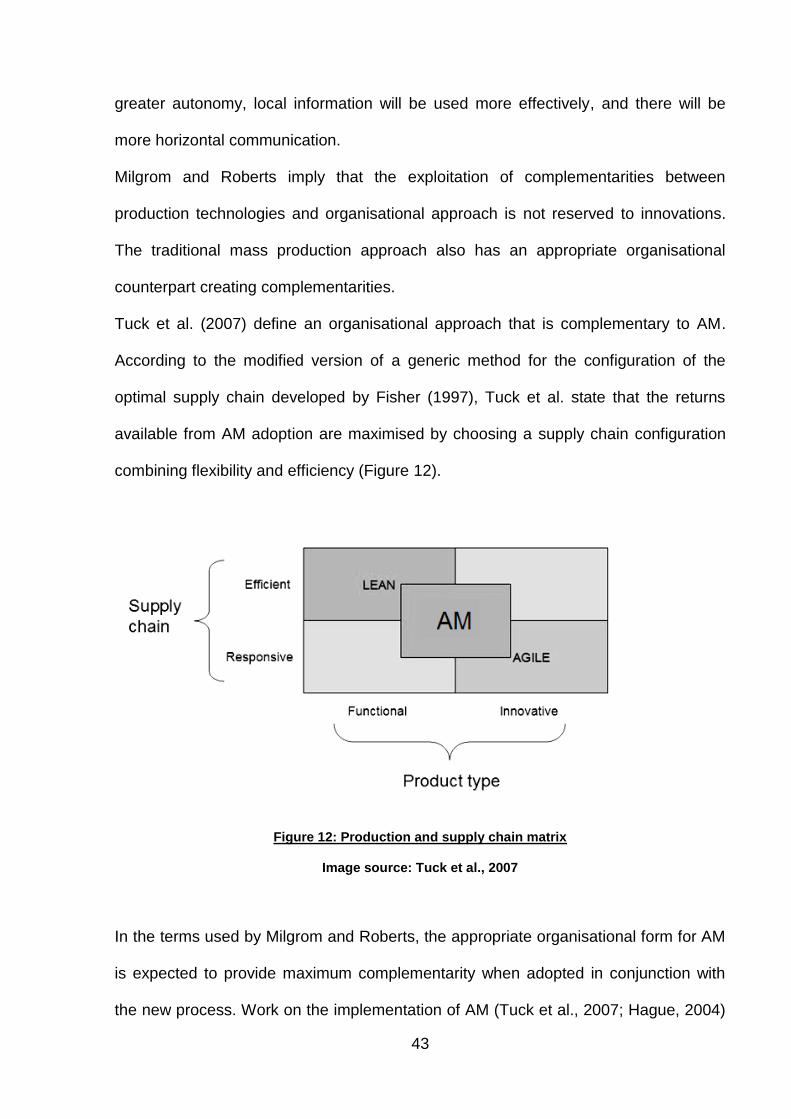
43

greater autonomy, local information will be used more effectively, and there will be

more horizontal communication.

Milgrom and Roberts imply that the exploitation of complementarities between

production technologies and organisational approach is not reserved to innovations.

The traditional mass production approach also has an appropriate organisational

counterpart creating complementarities.

Tuck et al. (2007) define an organisational approach that is complementary to AM.

According to the modified version of a generic method for the configuration of the

optimal supply chain developed by Fisher (1997), Tuck et al. state that the returns

available from AM adoption are maximised by choosing a supply chain configuration

combining flexibility and efficiency (Figure 12).

Figure 12: Production and supply chain matrix

Image source: Tuck et al., 2007

In the terms used by Milgrom and Roberts, the appropriate organisational form for AM

is expected to provide maximum complementarity when adopted in conjunction with

the new process. Work on the implementation of AM (Tuck et al., 2007; Hague, 2004)

44

suggests that a number of accompanying organisational changes need to be made to

reap the full benefits of the new technology. The following four aspects of

organisational change have been identified as suitable accompaniments to AM

technology adoption (Tuck et al., 2007):

Supply chain dematerialisation

The transmission of 3D CAD part data (which forms a complete representation

of the final part) through data networks reduces the requirement to physically

move intermediate inputs or final products. The idea is to dematerialise the

supply chain and perform a re-materialisation step using AM technology. This

should produce significant economic savings as it eliminates the need to

physically move intermediate products. Foran et al. (2005) comment that

modern supply chains can be extremely complex.

Just-in-time delivery

AM adoption may reduce warehousing and stock holding costs, as well as the

amount of capital tied up in work in progress. It is predicted that these changes

may lead to the replacement of the Just-in-Time delivery strategy by a novel

strategy of Just-in-Time manufacture. Positive by-products of this change could

be fuel and energy savings due to the elimination of transportation and stock

holding.

Increased manufacturing flexibility

Increased manufacturing flexibility allows reductions in set up times and part

count reduction: a minimised usage of labour inputs changes the composition

45

of total inputs compared to conventional manufacturing. This is associated with

decreasing logistical requirements due to the reduction of overall part count.

Elimination of waste

According to Tuck et al., the minimisation of generated waste is a principle of

the conventional lean manufacturing approach. Adoption of AM in conjunction

with accompanying process innovations may provide further waste reduction

potential in manufacturing and distribution. As discussed in this thesis in the

context of the possibilities afforded by geometric freedom, AM adoption may

result in very low raw material wastage. This may lead to significant

improvements in the environmental footprint of durable goods, especially when

constructed using an energy intensive raw material such as titanium, as

discussed in section 7.2.3.

Furthermore, AM may contribute to the phenomenon of dematerialisation, as

suggested by Tuck et al. in the context of virtual supply chains. Kander (2005) offers a

useful explanation of the term „dematerialisation„: it is understood to be a

microelectronics-driven move away from the traditional mode of production, to more

sustainable economic activity, fundamentally increasing the productivity of natural

resource inputs. The term dematerialisation has also been defined by Maxwell and

Van der Vorst (2003) as a process in which “the material and energy inputs into a

product are reduced or replaced completely by an immaterial substitute for complete

dematerialisation”.

46

2.2 Benefits of AM

2.2.1 Value creation in AM

Product life cycle assessment can be used to structure the various stages in the life of

a durable good, which, according to Waldman (2003) provides a stream of services

throughout its useful life. Interestingly, this framework can also be used as a starting

point in an analysis of the benefits made available through AM‟s freedom of geometry,

described as a capability of creating virtually any shape or geometry (Hague et al.,

2003; Rosen, 2007).

The environmental foot-printing specification PAS 2050:2011 (British Standards

Institutions, 2011) provides an overview of the various stages in the product life cycle,

as shown in Figure 13. According to this framework, the „cradle-to-grave‟ life cycle of a

durable good can be divided into distinct stages: an initial raw material generation

stage, a manufacturing stage, a distribution and retail stage, the actual use phase of

the product, and a final disposal stage.

Figure 13: The „cradle-to-grave‟ product life cycle, according to PAS 2050:2011

Image source: adapted from British Standards Institution (2011)

For a judgement on the combination of production process, design and material in the

production of durable goods, all costs arising to the user must be taken into account -

47

this includes the purchasing price at the transaction point (usually between distribution

and the use phase) and all operating expenses incurred during the use phase and the

costs of disposal after decommissioning.

The user will favour the combination that provides the maximum cumulative stream of

benefits to the user net of all costs. For a meaningful evaluation of costs and benefits

arising in the future it is imperative that these be discounted to net present value

(NPV). A summary of the methods used to discount future sums to NPV is given by

Hoy et al. (2001).

In contrast to the break-even costing approach suggested by Ruffo et al. (2006b), this

thesis argues that design can not be treated as fixed in inter-process comparisons if

the whole product life cycle is taken into account. Benefits yielded by process-borne

improvements in design may, during various stages in the product life cycle, offset

higher manufacturing cost for AM products.

Similar to the aspect of product differentiation in the model presented by Wong et al.

(2008), an aspect of economic behaviour is included when decisions are based on the

product life cycle: the buyer (or user) must factor in future operating cost, discounting

rates, acquisition cost, and where applicable, future costs of disposal (Dreyfus and

Viscusi, 1995).

2.2.2 DFM and a philosophy of design for AM

Bralla (1998) states that designers have historically focused on three factors:

functional performance, technical features and aesthetical appearance. Essentially,

the methodology of design for manufacturability (DFM) aims to enable the evaluation

of competing designs “so that the best approach can be chosen easily with the

assurance that it truly is the best one” (Bralla, 1998).

48

This position underlines the importance placed on manufacturability and low

manufacturing cost by engineering designers. DFM is a tool to make normative

judgements on part design: the design featuring the lowest manufacturing cost is

perceived to provide the greatest value and is hence favoured. However, product

performance characteristics have always been at the centre of considerations arising

further „downstream‟ such as serviceability, environmental friendliness and

ergonomics.

As established in section 2.2.1, the performance of durable goods is determined by

the cumulative flow of net benefits derived by the user. Due to DFM‟s emphasis on the

manufacturing process, its application may well produce ambiguous results in this

area. For the purpose of illustration consider the following example: in the

development of a part for use in an automotive application, initial specifications are

defined. Following this, the part is designed for minimum weight. DFM rules are then

applied and the conflicting discovery is made that a heavier design is required for a

low cost manufacturing process. In consequence, the design is altered according to

DFM and the weight of the final design exceeds the weight of the original design. The

hidden price of the increased weight may be that future users face higher operating

costs through increased fuel consumption. This example shows that while the

application of DFM is aimed at minimising manufacturing cost, the procedure may well

have an unintended and detrimental effect on the benefit stream derived during the

part‟s use phase.

To incorporate selected downstream effects of design decisions, and thereby reducing

the myopia inherent to DFM, Bralla proposes a knowledge-based „design for X‟ (DFX)

methodology that aims “to maximise all desirable characteristics – such as high

quality, reliability, serviceability, safety, user friendliness, environmental friendliness,

49

and short time-to-market – in a product design, while at the same time minimizing

lifetime costs, including manufacturing costs”.

In the analysis of geometrically less restrictive manufacturing techniques such as AM,

it appears useful to build models and decision tools directly taking into account the net

benefit stream yielded during the use phase. But which normative statements can be

made about good engineering design where geometrically less restrictive technology

is considered? Acknowledging AM‟s ability to manufacture almost any 3D content

generated with a CAD package, Hague et al. (2004) argue that “one is entering a new

dimension of „manufacture for design‟ rather than the more conventional DFM

philosophy”.

At this point it is necessary to acknowledge that the geometric freedom of AM is also

within limits (Hague et al., 2003; Gibson et al., 2010). Of course there are restrictions

on the geometries that AM technology can produce and these vary with the limitations

of individual AM technology variants. For example, in the SLM processes, parts need

to be anchored to the substrate to prevent deformation and dissipate heat. Further

problems arise from the support structures needed in some processes, for example for

FDM or Stereolithography. Perhaps the most obvious restriction in most additive

processes is that there is a maximum build envelope limiting part size.

In an attempt to make statements on what constitutes beneficial design and hence

maximises part functionality, a judgement on the „direction‟ of design improvements is

needed, informing on how a best solution which maximises benefits to users (and

ultimately functionality) can be found.

Flusser (1999) offers an approach to this problem in his analysis of the nature of

design. In his effort to illuminate why the word “design” has such great significance in

the modern world, Flusser examines the etymology of the term, derived from Latin:

50

“de-“, and “signum”. He finds meanings such as “intention”, “plan”, “aim”, “scheme” or

“plot”‟. He notes that the word occurs “in contexts associated with cunning and deceit.

A designer is a cunning plotter laying his traps” (Flusser, 1999).

Other terms, relevant in the context of engineering, fall into the same category:

“mechanics” and “machine” both originate from the Greek word “mechos”, meaning a

device designed to deceive – also a trap. The word “technology” originates from the

Greek “techne”, meaning “art”, closely related to tekton, which means “carpenter”. It is

explained how these meanings, which all have connotations with deception, stem from

ancient Greek epistemology (Flusser, 1999):

“The basic idea here is that wood […] is a shapeless material to

which the artist, the technician, gives form, thereby causing the form

to appear in the first place. Plato‟s basic objection to art and

technology was that they betray and distort theoretically intelligible

forms („Ideas‟) when they transfer these into the material world. For

him, artists and technicians were traitors to Ideas and tricksters

because they cunningly seduced people into perceiving distorted

ideas.”

According to Flusser, ancient Greek engineers took the view that designers and

engineers interpret platonic ideas and idealised forms. Incidentally, this platonic view

also provides a solution to the problem of defining the best design: a design can be

classified as superior to another design if it is closer to a hypothetical idealised design,

delivering maximum conceivable functionality and hence generating maximum utility

for its user.

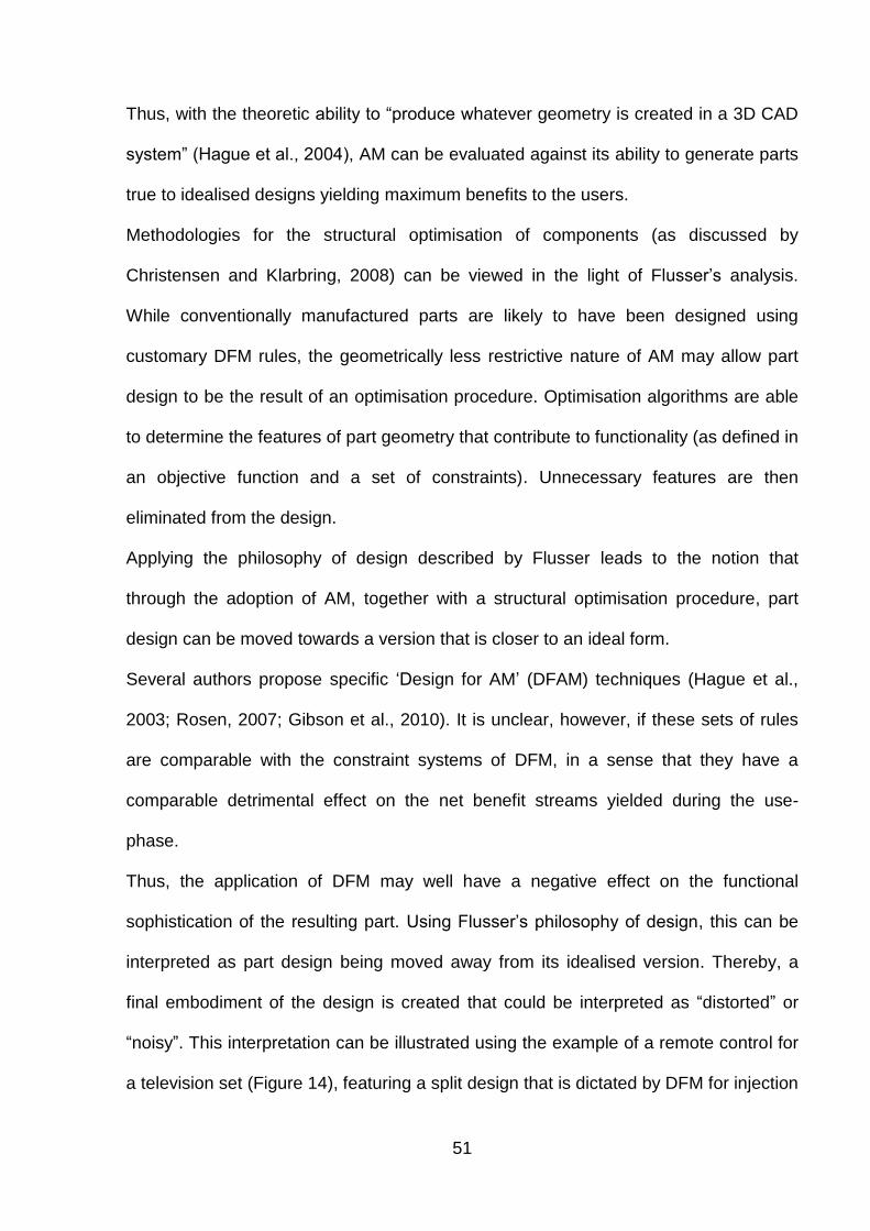
51

Thus, with the theoretic ability to “produce whatever geometry is created in a 3D CAD

system” (Hague et al., 2004), AM can be evaluated against its ability to generate parts

true to idealised designs yielding maximum benefits to the users.

Methodologies for the structural optimisation of components (as discussed by

Christensen and Klarbring, 2008) can be viewed in the light of Flusser‟s analysis.

While conventionally manufactured parts are likely to have been designed using

customary DFM rules, the geometrically less restrictive nature of AM may allow part

design to be the result of an optimisation procedure. Optimisation algorithms are able

to determine the features of part geometry that contribute to functionality (as defined in

an objective function and a set of constraints). Unnecessary features are then

eliminated from the design.

Applying the philosophy of design described by Flusser leads to the notion that

through the adoption of AM, together with a structural optimisation procedure, part

design can be moved towards a version that is closer to an ideal form.

Several authors propose specific „Design for AM‟ (DFAM) techniques (Hague et al.,

2003; Rosen, 2007; Gibson et al., 2010). It is unclear, however, if these sets of rules

are comparable with the constraint systems of DFM, in a sense that they have a

comparable detrimental effect on the net benefit streams yielded during the use-

phase.

Thus, the application of DFM may well have a negative effect on the functional

sophistication of the resulting part. Using Flusser‟s philosophy of design, this can be

interpreted as part design being moved away from its idealised version. Thereby, a

final embodiment of the design is created that could be interpreted as “distorted” or

“noisy”. This interpretation can be illustrated using the example of a remote control for

a television set (Figure 14), featuring a split design that is dictated by DFM for injection

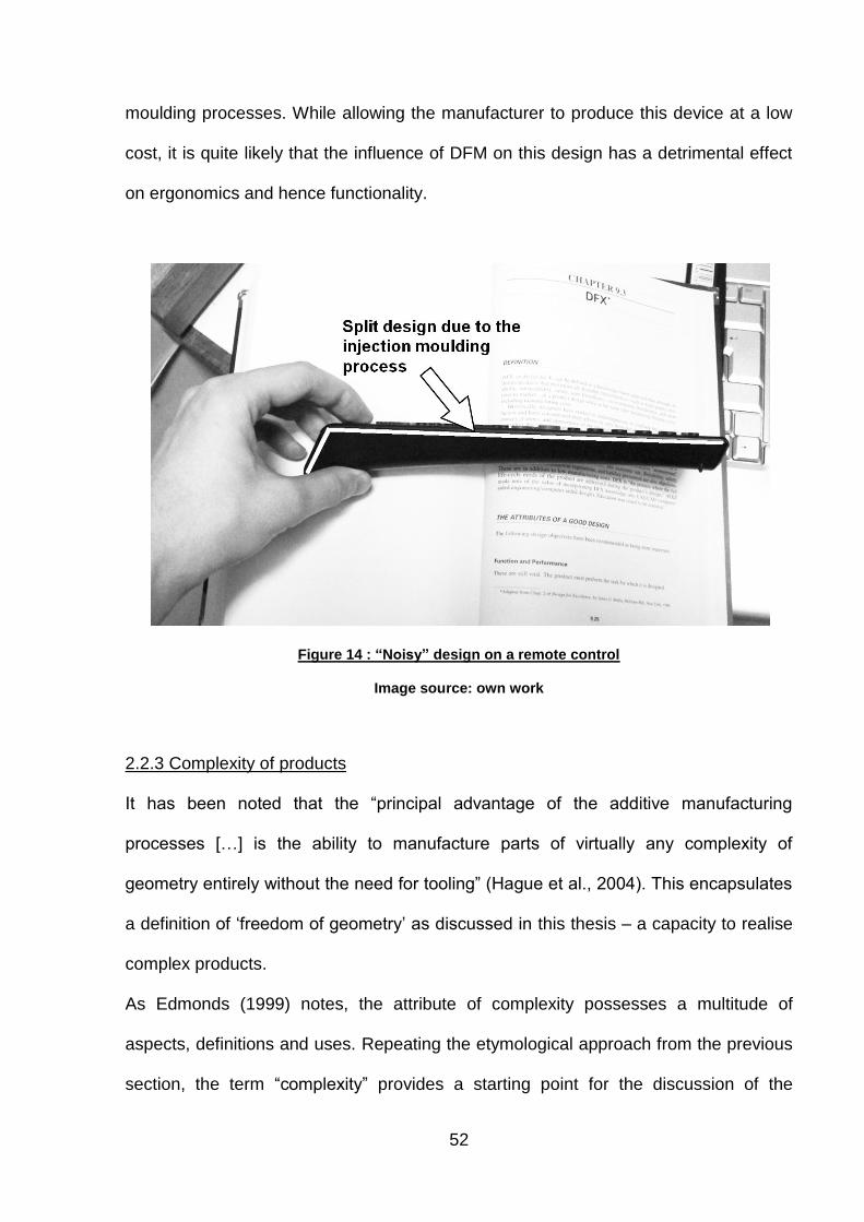
52

moulding processes. While allowing the manufacturer to produce this device at a low

cost, it is quite likely that the influence of DFM on this design has a detrimental effect

on ergonomics and hence functionality.

Figure 14 : “Noisy” design on a remote control

Image source: own work

2.2.3 Complexity of products

It has been noted that the “principal advantage of the additive manufacturing

processes […] is the ability to manufacture parts of virtually any complexity of

geometry entirely without the need for tooling” (Hague et al., 2004). This encapsulates

a definition of „freedom of geometry‟ as discussed in this thesis – a capacity to realise

complex products.

As Edmonds (1999) notes, the attribute of complexity possesses a multitude of

aspects, definitions and uses. Repeating the etymological approach from the previous

section, the term “complexity” provides a starting point for the discussion of the

53

relevance of the concept of complexity in the area of the economics of AM. In Latin,

the term “complexus” forms the past participle of the verb “complectere”, which can be

translated as “to embrace, to comprise” (Oxford Dictionaries, 2011). This, in turn,

consists of the prefix “com-“ (“with”) and the verb “plectere” (“to weave”, “to braid”, “to

twine”). Thus, the origin of the word indicates that the term refers to an attribute of

difficulty in the separation of constituting elements of some whole.

A useful division line in the domain of complexity appears to be the distinction

between the complexity of a geometry and the complexity of topology. However, in

this thesis a definition of the term complexity is avoided. Instead, this work aims to

quantify aspects that are subjectively associated with a shape‟s or product‟s

complexity.

Through the adoption of AM, the requirement to minimise part complexity, as

formulated in the DFM literature, is removed. Moreover, Hague et al. (2003) suggest

that in conventional manufacturing, there is a direct link between the complexity of a

design and its cost. This results in an economic imperative to minimise the complexity

of a design. Using AM however, “it is effectively possible to obtain the geometry (or

complexity) for „free‟ [...]” (Hague et al., 2003), eliminating incentives to reduce the

complexity of a design out of cost or manufacturability considerations.

Therefore, comparing AM with conventional processes a gap in average cost (AC)

may open as the complexity of a design increases. This is possible because the

marginal cost of extra complexity is potentially zero where AM is employed, as

illustrated in Figure 15.

54

Figure 15: Marginal cost of complexity

Image source: own work

However, the feature of such costless extra complexity may not be exclusive to AM. A

similar mechanism has been observed in the production economics of the

semiconductor industry. In the manufacturing of integrated circuitry, the nature of the

employed photolithographic process may allow the inclusion of extra logical elements

at zero cost (Schaller, 1997), depending on the configuration. Here, technological

evolution has enabled both great advances in product performance and reductions in

cost, regularly exceeding the most optimistic predictions of technology experts

(Schnaars, 1994).

According to a well-known paper by Moore (1965), advances in computing power are

enabled by an increased density of logical components in integrated circuits. The

nature of the employed photolithographic process implies that the addition of more

logical elements does not necessarily come at an increased manufacturing cost. In

principle, the pure manufacturing cost associated with the lithographic production of

an integrated circuit appears to be independent of its geometric layout and complexity.

55

As for AM, there may be no direct causal link between design complexity and

manufacturing cost.

However, it should be noted that Ruffo et al. (2006a) demonstrate that (maintaining

the same part volume and part height) a weak connection between part geometry and

laser scan time exists in AM. Whether this result should be interpreted as conflicting

with the notion of „freedom of geometry‟ expressed by Hague et al. (2004), needs to

be assessed.

The reported absence of geometric limitations in AM gives rise to a question about the

characteristics that should be considered in the identification of a best approach in the

future. As suggested in section 2.2.2, a rather abstract requirement can be derived

from durable goods theory: the best design will maximise the net stream of benefits

yielded. However, ex ante evaluations of entire product life cycles require extremely

rich datasets. Not only is a complete account of manufacturing costs necessary, it

further requires a credible projection of the use phase and of how design parameters

are connected to all operating and disposal costs.

Components for transportation applications allow limited statements of this nature.

The energy consumption during a vehicle‟s use-phase establishes an important link

between a vehicle‟s energy efficiency, which is heavily impacted by weight (Helms and

Lambrecht, 2006) and costs originating from fuel consumption. The mass of a vehicle

component is, of course, an important design parameter.

The same methodology can be applied in efforts to determine designs that feature the

minimum life cycle energy consumption. Whether the maximisation of the net stream

of benefits during a component‟s life also coincides with the minimisation of total life

cycle energy consumption is a highly important research question. In this context,

Lovins (1999) suggests that to improve energy efficiency, for example in

56

manufacturing, incentives must be aligned correctly in a sense that a configuration

with the minimal energy consumption must also minimise use-phase costs.

2.2.3.1 Quantification of shape complexity

As indicated in section 2.2.3, the term complexity can have numerous meanings. In

the engineering context, the measurement of shape complexity may be implemented

to pragmatically serve different purposes.

One notable example is its use as a tool for the specification of forging processes

(Tomov, 1999). To this end a measure of shape complexity is calculated, based on the

estimation of the work needed for material deformation during the forging process.

This thesis, however, follows another approach: the complexity of a shape is viewed

as a property that is experienced subjectively. Psarra and Grajewski (2001) discuss

the measurement of characteristics that are associated with the perception of such

complexity. Limiting the analysis to the properties of two dimensional shapes, which

are defined as “configurations consisting of edges and corners defining a continuous

perimeter line”, Psarra and Grajewski quantify characteristics associated with

complexity.

In their analysis, the degree of convexity of the perimeter shapes is the central

determinant and inversely related to the subjective quality of shape complexity. Full

convexity is defined by Psarra and Grajewski as property that every point in the

perimeter can be connected to every other point without crossing the perimeter or

locations lying outside of the shape. Imagining the perimeter of the shape as opaque

walls, this carries the interpretation of occlusion, or non-visibility, as shown in Figure

16. Thus, in a convex shape, all points of the perimeter can be described as „visible‟

from every location.

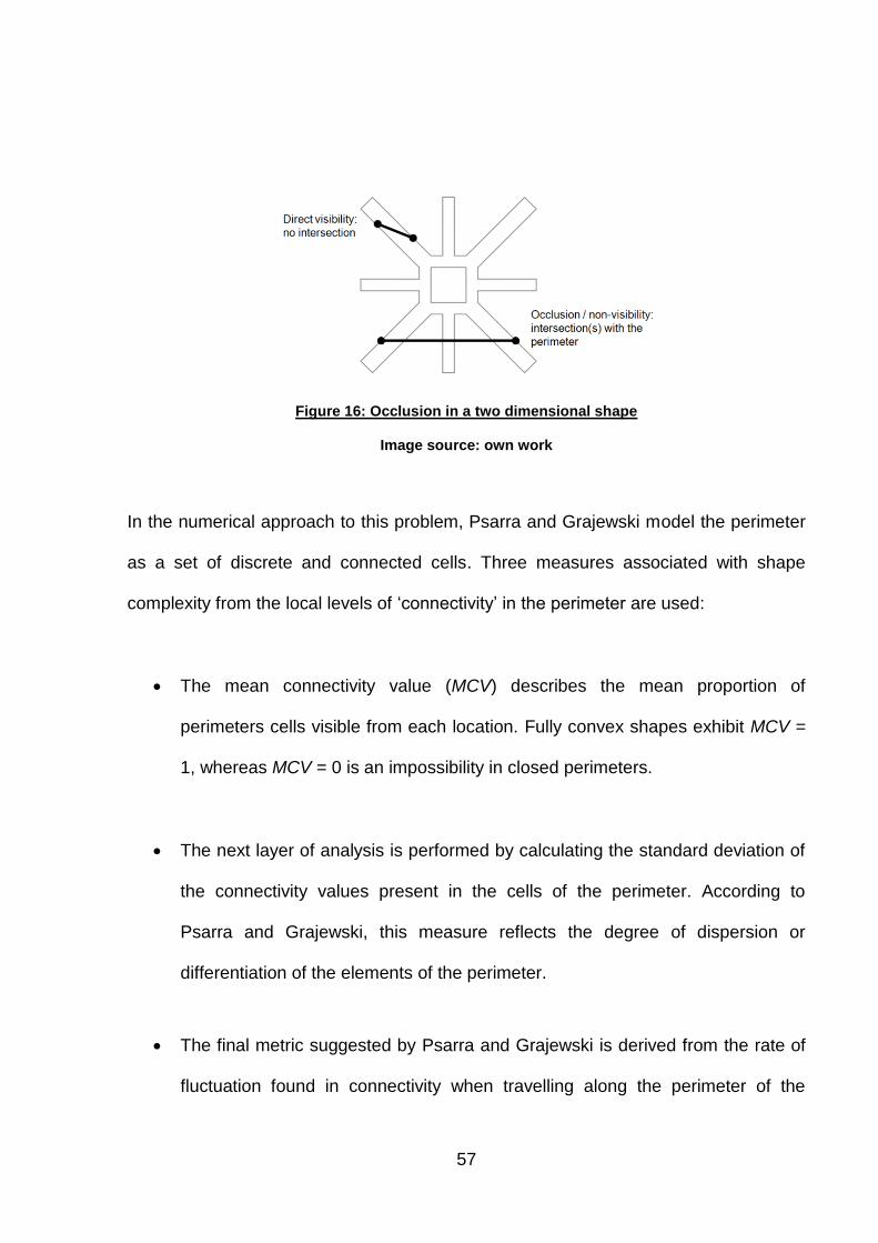
57

Figure 16: Occlusion in a two dimensional shape

Image source: own work

In the numerical approach to this problem, Psarra and Grajewski model the perimeter

as a set of discrete and connected cells. Three measures associated with shape

complexity from the local levels of „connectivity‟ in the perimeter are used:

The mean connectivity value (MCV) describes the mean proportion of

perimeters cells visible from each location. Fully convex shapes exhibit MCV =

1, whereas MCV = 0 is an impossibility in closed perimeters.

The next layer of analysis is performed by calculating the standard deviation of

the connectivity values present in the cells of the perimeter. According to

Psarra and Grajewski, this measure reflects the degree of dispersion or

differentiation of the elements of the perimeter.

The final metric suggested by Psarra and Grajewski is derived from the rate of

fluctuation found in connectivity when travelling along the perimeter of the

58

shape. This characteristic is captured by recording the horizontal distance

between the intersections of the graph of connectivity with the MCV line. Psarra

and Grajewski then measure the standard deviation of this distance to arrive at

a measure that describes the degree of fragmentation, repetitiveness or rhythm

present in the shape.

Specifically, these three metrics are presented as a way of quantifying the subjective

experiences resulting from floor plans of buildings. However, this method is

transferrable to the measurement of the occlusion characteristics of three dimensional

surfaces. This thesis takes the position that this forms a relatively simple and

pragmatic way to grasp the property of shape complexity of engineering designs.

2.3 AM productivity, energy consumption and cost

After summarising various items of economics-related background literature and the

literature helpful for the discussion of the benefits arising from AM usage, the last

component of this literature review presents the existing body of work on the

measurement of AM system productivity, energy consumption, manufacturing cost,

and build volume utilisation.

To avoid confusion arising from different measurement units and currencies, this

review will report relevant results from the literature in their native unit. This applies in

particular to the unit of data measuring for electrical energy, which are reported in kWh

and MJ, where 1Ws = 1 J, and hence 1 kWh = 3.6 MJ. However, MJ is preferred as

the measurement unit; it will be used exclusively in the sections following the literature

review. Monetary values are reported in nominal values in the currencies used in the

literature. The conversion of monetary values into 2010 pounds sterling (£), which is

59

the preferred monetary unit in this thesis, is explained in the methodology section

3.3.3.5.

2.3.1 Build time estimation

Commercially available rapid prototyping software packages contain build time

estimation functionality (Campbell et al., 2008), as do the machine software suites

sold in bundles with additive systems (Ruffo et al., 2006a).

Offering a framework for the classification of AM build time estimators, Di Angelo and

Di Stefano (2011) argue that the existing approaches can be divided into „detailed-

analysis‟ methods based on detailed knowledge of the inner workings of AM systems

and „parametric‟ methods informed by data on a set of process characteristics such as

layer thickness, hatch distance, and laser scan velocity. The developed build time

estimation approaches are normally designed for particular AM technology variants.

A detailed-analysis approach to the time estimation problem for Stereolithography

(SLA) is presented by Chen and Sullivan (1996), showing that the specifics of the

laser scanning technique, including scan speed, laser power, spot size and scanning

strategy can be used to predict build time. Further parameters that flow into this

estimator are the time consumed for vertical platform dip/re-raise and wiper activity, as

well as unspecified hardware delays. While the build time estimator proposed by Chen

and Sullivan does not employ data on actual part geometry, the authors comment that

the use of such data is advantageous.

Giannatsis et al. (2001) present a similar estimator for SLA, using variables such as

contour length, hatch area, scan speed and resin properties. The authors present two

different implementations of their estimator for use with data on part geometry. The

first variant interrogates data on product geometry in the *.stl file format, which

60

represents the standard file format for the exchange of part data amongst AM users

and for communication with additive machinery. In a second variant, Giannatsis et al.

present an implementation using pre-sliced data in the *.cli format, representing

individual layers, for which more accurate results are reported.

Analogous to the incremental addition of layers of geometry in additive processes,

Giannatsis et al. express build time as the sum of the time consumed to deposit each

layer:

∑ (Eq. 3)

where TLayeri is the time consumed to deposit the „i‟th layer of a total of „n‟ layers.

Giannatsis et al. model TLayeri as the sum of the time consumed by the additive

system for recoating the new layer TRecoati with photosensitive resin and the time

spent by the optical system for the scanning of the layer, TScani:

(Eq. 4)

The constituents of time consumption for recoating TRecoati and scanning TScani are

defined by Giannatsis et al. as the product of further underlying process elements,

such as wiper speed, scanning velocity, beam diameter and curing depth.

A further detailed analysis of build time estimation is presented Byun and Lee (2006),

discussing the AM technology variants SLA and FDM. Byun and Lee introduce a

framework of relationships governing build time, similar to the approach presented by

Giannatsis et al. (2001). By discussing the constituents of time consumption for both

SLA and FDM, Byun and Lee show how these relationships vary across different

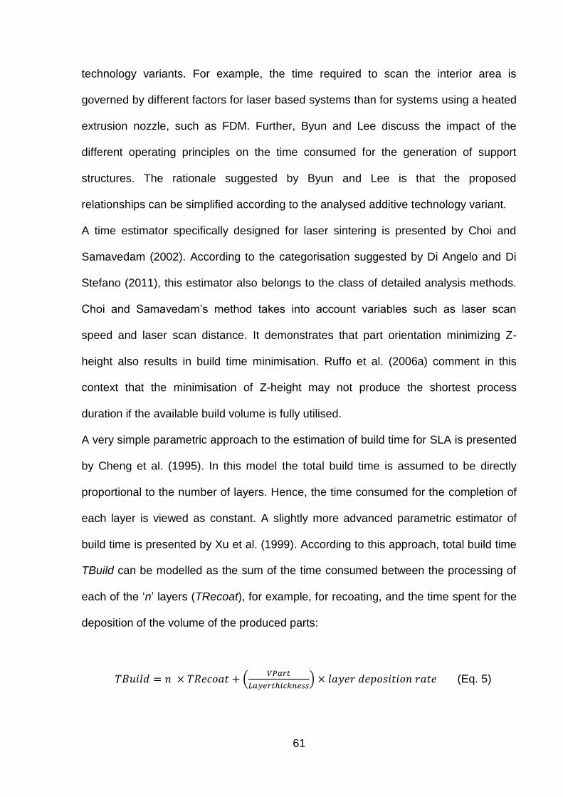
61

technology variants. For example, the time required to scan the interior area is

governed by different factors for laser based systems than for systems using a heated

extrusion nozzle, such as FDM. Further, Byun and Lee discuss the impact of the

different operating principles on the time consumed for the generation of support

structures. The rationale suggested by Byun and Lee is that the proposed

relationships can be simplified according to the analysed additive technology variant.

A time estimator specifically designed for laser sintering is presented by Choi and

Samavedam (2002). According to the categorisation suggested by Di Angelo and Di

Stefano (2011), this estimator also belongs to the class of detailed analysis methods.

Choi and Samavedam‟s method takes into account variables such as laser scan

speed and laser scan distance. It demonstrates that part orientation minimizing Z-

height also results in build time minimisation. Ruffo et al. (2006a) comment in this

context that the minimisation of Z-height may not produce the shortest process

duration if the available build volume is fully utilised.

A very simple parametric approach to the estimation of build time for SLA is presented

by Cheng et al. (1995). In this model the total build time is assumed to be directly

proportional to the number of layers. Hence, the time consumed for the completion of

each layer is viewed as constant. A slightly more advanced parametric estimator of

build time is presented by Xu et al. (1999). According to this approach, total build time

TBuild can be modelled as the sum of the time consumed between the processing of

each of the „n‟ layers (TRecoat), for example, for recoating, and the time spent for the

deposition of the volume of the produced parts:

(

) (Eq. 5)

62

As Di Angelo and Di Stefano (2011) note, the model by Xu et al. is a simple

specification, unable to account for the effect of part geometry and unable to reflect

unproductive time caused by laser/tool positioning.

Identifying the main drivers of laser sintering build time as Z-height, part volume and

the size of the bounding box, Ruffo et al. (2006a) present a build time estimator that is

able to take into account aspects of part complexity. The model for build time

suggested by Ruffo et al. is similar to the above in that it views total build time as the

sum of a number of process elements.

According to Ruffo et al., the constituents of total build time, TBuild, are: total scanning

time TScan, total recoating time TRecoat, and time consumed for build preparation

and post processing, TPrep:

(Eq. 6)

The time estimator shown in Equation 6 views the time spent for recoating as a

constant and independent of part geometry. Further, the time consumed by the

additive system for scanning is modelled as dependent on the density of the parts

within their bounding box, also providing a rough proxy for part complexity.

This follows the intuition that a simple part should exhibit a shape that conforms to its

cuboid bounding box relatively well, producing a relatively high density, or „compact

ratio‟ (Ruffo et al., 2006a). Vice versa, a more complex part, which does not fit well

into its bounding box, is expected to show a low compact ratio.

Di Angelo and Di Stefano (2011) criticise that the model proposed by Ruffo et al. is

applicable only to LS and is not easily transferrable to AM technology variants

requiring the use of support structures.

63

Ruffo et al. report the maximum estimation error for their polymeric LS time estimator

at 13%. This value could not be reconstructed with data from the four reported

configurations provided by Ruffo et al. (2006a). These suggest a mean absolute

estimation error of 9.85%. Wilson (2006) proposes a similar parametric multi-platform

cost estimation model sharing the initial build time model with Ruffo et al. (2006a).

A further parametric approach to the problem of AM build time estimation for the

technology variant SLA is proposed by Campbell et al (2008). This model explores

whether geometrical primitives, such as spheres, cylinders and cones, can be used in

build time estimation if actual part geometry in the *.stl format is not available. The

parametric model for scan time estimation per layer proposed by Campbell et al. is:

(Eq. 7)

where ALayer is the area cured per layer, Hatch spacing describes the distance

between the individual laser scan paths and Vs denotes the scan velocity. It should be

noted that this approach does not distinguish between contour scanning and hatch

scanning and that recoating time is assumed to be constant. Campbell et al. draw the

conclusion that hatch scanning time in SLA is directly proportional to the cross

sectional area and inversely proportional to laser output. The authors compare the

accuracy of their estimator to the performance of the commercial software package

Magics RP (Version 6.3), citing a mean percentage error of 3.8%.

However, the reported error is not indicative of estimator performance as positive and

negative errors in the calculation presented by Campbell et al. cancel each other out.

Using the data provided, the mean absolute estimation error can be calculated at

64

8.69%. Moreover, Campbell et al. present a mean estimation error of -4.54% for their

own estimator.

Munguia (2009) discusses the application of an artificial neural network (ANN)

technique to the build time estimation problem for AM technology variants LS and

SLM. Munguia describes ANNs as a non-parametric methodology devised to “fit

curves through data without being provided a predetermined function with free

parameters [and] therefore [...] able to detect hidden functional relationships”.

Munguia comments that the unavailability of build time estimators for metallic AM

technology variants may be due to competitive behaviour exhibited by AM control

software authors or due to the idiosyncrasies connected to the post processing of

metal parts. For the ANN build time estimator, Munguia reports a high degree of

accuracy, citing a mean estimation error of 2.8% in a sample of parts. Interestingly,

Munguia also applies the build time estimators devised by Ruffo et al. (2006a) and

Wilson (2006), reporting mean errors of 14.98% and 22.68%, respectively.

Di Angelo and Di Stefano (2011) present a further, ANN-based build time estimator

usable for different AM technology variants. Applying this estimator to the AM

technology variant 3D printing, the authors report a mean estimation error of 12%.

To summarise, the existing work on AM build time estimation can be classified into

parametric approaches (Cheng et al., 1995; Xu et al., 1999; Ruffo et al., 2006a;

Wilson, 2006; Campbell, 2008) and detailed-analysis techniques (Chen and Sullivan,

1996; Giannatsis et al., 2001; Choi and Samavedam, 2002; Byun and Lee, 2006). The

„learning‟ ANN methodology carries the advantage of not needing a functional

specification to begin with (Munguia, 2009; Di Angelo and Di Stefano, 2011). The

disadvantage of the ANN method is the need for large datasets to enable precise

results.

65

The approach proposed by Giannatsis et al. (2001) stands out because is assesses

actual part geometry in the *.stl file format. In terms of the build time estimator

performance reported in this review, no estimation technique appears to be

unambiguously superior. However, as noted by Chen and Sullivan (1996), the use of

part geometry contributes to model accuracy.

2.3.2 AM energy consumption

A precise understanding of the emissions associated with available manufacturing

processes is fundamental to decision making towards sustainability in the

manufacturing sector. The measurement of such emissions forms an important area of

research in the field of industrial ecology, where a variety of methods are employed to

analyse the interactions between human activity and the environment (Gößling-

Reisemann, 2008). In particular, the quantification of carbon emissions, referred to as

„carbon accounting‟, requires a precise understanding of the energy flows associated

with production processes (Vijayaraghavan and Dornfeld, 2010).

As argued in the introduction to this thesis, the consequences of carbon emissions

arise to society as a whole, not exclusively to those responsible for the pollution.

Therefore, these consequences are described as social costs. As Romer (2001)

notes, the appropriate policy to deal with carbon emissions is clear: the social cost of

pollution, for example from rising sea levels or changes in weather patterns, should be

measured in money terms and the polluters should be taxed accordingly. This is of

course not possible. A starting point however, is the measurement and estimation of

the electric energy consumed by manufacturing processes.

As discussed by Kellens et al. (2012), data on manufacturing process productivity,

energy consumption, consumables usage and emissions are fundamental to the

66

ecological impact occurring in manufacturing. Due to the CO2 emissions associated

with electric power usage (Jeswiet and Kara, 2008), the measurement of process

energy consumption forms a cornerstone in life cycle analyses of the impact of

products. In specific, such measurements contribute to inventory analysis, which

compiles all energy and material flows throughout the life cycle (Jiménez-González

and Overcash, 2000).

In an initial study of AM power consumption, Luo et al. (1999) compare the

environmental impact of three major polymeric additive technology variants (SLA,

FDM and LS). Luo et al. evaluate the impact during actual production activity.

According to Luo et al., the process elements of relevance during this stage are

energy consumption and the generation of waste residue. It is further suggested that

the environmental impact of process residues are negligible, their paper concentrates

on energy consumption.

The energy consumption characteristics reported by Luo et al. for each system are

based on a mean power consumption value P, measured in kW, and a number of

parameters characterising the additive system and the build material:

V - Scanning/drawing velocity (in mm per s)

W - Beam/deposition width (in mm)

T - Layer thickness (in mm)

ρ - Material density (in kg per mm³)

k - Process overhead coefficient

The summary metric of specific energy consumed per kg of material deposited (SE) is

then approximated:

67

(Eq. 8)

Two aspects of this simple methodology are noteworthy: while V, W, T and ρ describe

very basic parameters on material deposition during the processes, they do not carry

information on energy consumption. All information on process efficiency is contained

in the parameters k and P. The information on both parameters appears to have been

empirically collected. Luo et al. state that most of the data used originate from PRê

Consultants (2011). Table 1 summarises the energy consumption metrics reported by

Luo et al. for the three assessed AM technology variants:

Table 1: Major AM technology variants analysed by Luo et al. (1999)

Stereolithography LS FDM

Mean power consumption 1.2 – 3.0 kW 12.5 – 16.8 kW 1.32 – 11.0 kW

Specific energy consumption per kg deposited

20.70 – 41.38 kWh 29.83 – 40.09 kWh 23.08 – 346.4 kWh

In a similar framework, Sreenivasan and Bourell (2009) study power consumption of

LS. Apart from reporting the specific energy consumption per kg of material deposited,

14.5 kWh, the authors also cite mean power consumption of the investigated LS

system, a 3D Systems Sinterstation HS+HiQ. It is measured empirically at 19.6 kW

over the investigated build.

A further study of AM energy consumption assessing multiple AM technology variants

is provided by Mognol et al. (2006). The authors investigate the power consumption of

both polymeric (3D printing and FDM) and metallic AM systems (DMLS). It is

demonstrated that part orientation in a system‟s internal build volume can affect

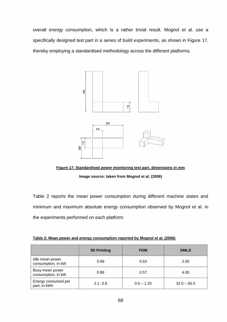
68

overall energy consumption, which is a rather trivial result. Mognol et al. use a

specifically designed test part in a series of build experiments, as shown in Figure 17,

thereby employing a standardised methodology across the different platforms.

Figure 17: Standardised power monitoring test part, dimensions in mm

Image source: taken from Mognol et al. (2006)

Table 2 reports the mean power consumption during different machine states and

minimum and maximum absolute energy consumption observed by Mognol et al. in

the experiments performed on each platform:

Table 2: Mean power and energy consumption reported by Mognol et al. (2006)

3D Printing FDM DMLS

Idle mean power consumption, in kW

0.69 0.53 2.00

Busy mean power consumption, in kW

0.88 0.57 4.00

Energy consumed per part, in kWh

2.1 -3.8 0.5 – 1.25 32.0 – 56.0

69

Kellens et al. (2010b) provide a further multi-platform study of AM energy

consumption, reporting energy consumption of polymeric LS and the metallic

technology variant SLM. Unlike the study by Mognol et al. (2006), the authors report

energy consumption results for full build experiments holding multiple units of end-use

parts. Table 3 reports the mean power and energy consumption results reached by

Kellens et al. (2010b) for four different additive systems:

Table 3: Mean power consumption reported by Kellens et al. (2010b)

Technology variant LaserCusing LS

Machine type ConceptLaser

M3 Linear EOSINT P760 EOSINT P360

EOSINT Formiga P100

Idle and product removal

0.7 kW 3.52 kW 2.25 kW 0.34 kW

Preheating and atmosphere generation

2.25 kW 8.28 kW 4.00 kW 2.96 kW

Build (exposure) 3.25 kW 6.61 kW

3.74 kW 1.30 kW

Build (recoating) 3.45 kW 5.31 kW

Kellens et al. further provide estimates on specific energy consumption on the largest

LS system assessed, the EOSINT P760, presenting results for three different layer

thickness / build material combinations. Using data presented by Kellens et al.

(2010a), a specific energy consumption value of the surveyed Concept Laser M3

Linear “LaserCusing” system can be approximated at 26.89 kWh per kg of material

deposited. The energy consumption results observed by Kellens et al. (2010a; 2010b)

are summarised in Table 4.

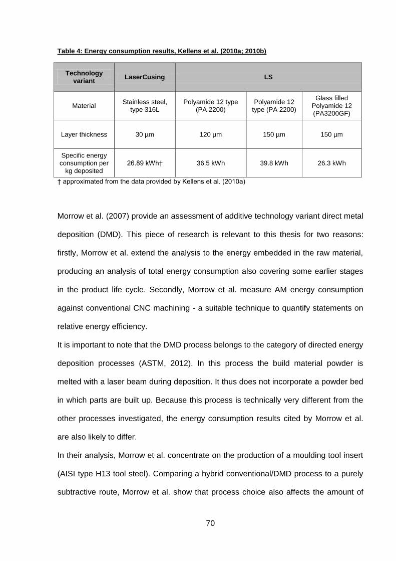
70

Table 4: Energy consumption results, Kellens et al. (2010a; 2010b)

Technology variant

LaserCusing LS

Material Stainless steel,

type 316L Polyamide 12 type

(PA 2200) Polyamide 12

type (PA 2200)

Glass filled Polyamide 12 (PA3200GF)

Layer thickness 30 µm 120 µm 150 µm 150 µm

Specific energy consumption per

kg deposited 26.89 kWh† 36.5 kWh 39.8 kWh 26.3 kWh

† approximated from the data provided by Kellens et al. (2010a)

Morrow et al. (2007) provide an assessment of additive technology variant direct metal

deposition (DMD). This piece of research is relevant to this thesis for two reasons:

firstly, Morrow et al. extend the analysis to the energy embedded in the raw material,

producing an analysis of total energy consumption also covering some earlier stages

in the product life cycle. Secondly, Morrow et al. measure AM energy consumption

against conventional CNC machining - a suitable technique to quantify statements on

relative energy efficiency.

It is important to note that the DMD process belongs to the category of directed energy

deposition processes (ASTM, 2012). In this process the build material powder is

melted with a laser beam during deposition. It thus does not incorporate a powder bed

in which parts are built up. Because this process is technically very different from the

other processes investigated, the energy consumption results cited by Morrow et al.

are also likely to differ.

In their analysis, Morrow et al. concentrate on the production of a moulding tool insert

(AISI type H13 tool steel). Comparing a hybrid conventional/DMD process to a purely

subtractive route, Morrow et al. show that process choice also affects the amount of

71

energy embedded in the required raw material, due to different raw material

consumption. Morrow et al. report an embedded energy statistic of 20.41 MJ per kg of

H13 steel plate and 15.9 MJ per kg for H13 steel powder (from a direct atomisation

route).

Morrow et al. report the energy consumed during a single DMD manufacturing step in

which the mould geometry is built up on a metal substrate (also taking into account a

heat treatment procedure). This is compared to the conventional CNC route consisting

of rough and finish milling operations. For DMD, Morrow et al. cite a specific energy

consumption of 7708 MJ per kg of material deposited. Energy consumption during the

conventional five stage milling process is reported at 624 MJ per kg of part material

removed.

In the final step of their analysis, Morrow et al. combine the manufacturing process

energy consumption with the energy embedded in the raw materials. The results show

that the DMD route consumes in excess of 3000 MJ per part, compared to

approximately 57 MJ per part for the conventional milling pathway. This leads to the

conclusion that for minimum energy consumption, the conventional route would be

“the obvious choice” (Morrow et al., 2007).

Compared to other metallic additive platforms (Mognol et al., 2006; Kellens et al.,

2010b) the cited DMD energy consumption appears excessive. A possible reason can

be identified: the mean real power consumption reported for the DMD process (~ 61

kW) is much greater, this may indicate a measurement error. Further, the build

duration of the DMD experiment appears extensive (approximately 16 h). In this

context, Morrow et al. state that due to technical reasons, the DMD deposition rate

was set to the lowest possible configuration. Despite the “suboptimal” (according to

Morrow et al.) implementation of DMD, a much noticed paper by Gutowski et al.

72

(2009) uses these results to support a claim of increasing energy requirements of

manufacturing process innovations.

It can be concluded from this survey of available literature on AM energy consumption

that the specific energy consumption results can differ significantly, for AM in general

as well as for individual technology variants. Telenko and Seepersad (2010) suggest

in this context that differences in Z-height and packing density of the build experiments

are responsible. This supports the assumption that the degree of capacity utilisation is

very likely to have a bearing on energy requirements. Dedicated estimators of AM

energy consumption, analogous to the build time estimators presented in section

2.3.1, are not available in the literature.

2.3.3 Cost estimation

Son (1991) proposes a useful classification system for the various costs arising from

the use of advanced manufacturing machinery. It is suggested that costs can be

divided into “relatively well-structured costs”, reflecting items such as raw material,

labour, machine costs and overheads, and “relatively ill-structured costs”, including all

costs associated with build failure, error prevention, machine setup, waiting time,

idleness, and inventory. The work cited in this section concentrates on the analysis of

such well-structured costs arising during the AM processes.

Build time is an important driver of manufacturing cost for additive technologies.

Several authors construct costing models based on build time estimation

methodologies, as discussed in section 2.3.1 (Munguia, 2009; Di Angelo and Di

Stefano, 2008; Byun and Lee, 2006; Wilson, 2006; Alexander et al., 1998). This

review of the existing work on the monetary cost of AM, however, concentrates on two

73

items of the literature leading to particularly conflicting results, Ruffo et al. (2006b) and

an earlier study by Hopkinson and Dickens (2003).

To estimate the manufacturing cost of parts created with AM, Ruffo et al. show that an

activity based costing approach is viable. In their paper, Ruffo et al. suggest that the

increased level of automation associated with the adoption of AM should be reflected

in a model of manufacturing cost. The authors present a full costing approach that

divides the various costs arising into different activities. As argued by Atrill and

McLaney (1999), the challenge in implementing such costing models in capital

intensive contexts, such as AM, is to correctly apportion the indirect costs arising from

production.

In their model, Ruffo et al. initially determine an allocation base for these overheads.

For an estimate of an AM build‟s cost, the arising direct costs are added to a share of

the total annual indirect costs incurred by the AM user. Ruffo et al. determine the

share‟s size by estimating the time needed to complete the build, as discussed in

section 2.3.1.

Thus, Ruffo et al. propose an AM costing model viewing the total cost of a build, CBuild,

as the sum of all direct raw material costs and the indirect costs (Equation 9). The

direct costs are obtained by multiplying the mass of deposited material MBuild by the

cost of the raw material CMaterial (measured in € / kg). The indirect costs are calculated

by multiplying the total build time TBuild by an indirect cost rate ĊIndirect (measured in €

per s):

. (Eq. 9)

74

An estimate of cost per part CPart is then calculated by dividing CBuild by the number of

parts contained in the build nBuild.

Part geometry impacts the model through direct cost (determined by the amount of

raw material used) and the associated production time. The cost model is constructed

using a series of cost estimation relationships - part parameters such as Z-height and

part volume enter the indirect cost component through a separate production time

estimator (discussed by Ruffo et al., 2006a).

It is critical, however, that for an average cost estimate for each unit produced, Ruffo

et al. (2006b) implicitly introduce a second allocation base to the model. They suggest

that the realised total cost of a build should be divided by the number of parts

contained in that build. This carries two consequences that seriously impede the

model‟s ability to realistically estimate the cost of AM output.

The first consequence of this is that the model only applies to builds containing the

same geometry. In a critical evaluation of the model proposed by Ruffo et al. (2006b),

Ruffo and Hague (2007) state that the main limitation is an inability to account for the

production of build volumes containing more than one type of part – as a premise, the

production of identical parts is quite alien to the idea of AM being used to flexibly build

different parts in parallel. After all, it is a key advantage of AM “to simultaneously

produce numerous parts, say a complete assembly, on a single machine” (Hopkinson

and Dickens, 2003).

The second consequence of obtaining a unit cost estimate by simply dividing the build

cost by the number of parts requires greater elaboration. Due to a number of process

steps that are independent of the quantity of parts contained in the build, for example

warm up procedures, certain elements of fixed cost are incurred during every build on

the machinery. At low production quantity, these cannot be amortised over a

75

sufficiently large number of parts to produce low average costs. The saw-tooth shape

of the AM cost function observed by Ruffo et al. (2006b) suggests that each time a

new line, layer or build is added, average costs increase irregularly for some marginal

units. This is due to penalties in the form of increased raw material consumption and

process time.

Thus, Ruffo et al. (2006b) argue that the average cost curve for AM production is

initially downward sloping with a saw tooth shape at small production volumes and

then stabilises around some asymptotic value as production volume becomes large.

Figure 18 compares three versions of the model proposed by Ruffo et al. (2006b) to

the result reached by Hopkinson and Dickens (2003) and an injection moulding cost

function.

Figure 18: Comparison of AM average cost functions

Image source: Ruffo et al., 2006b

76

The saw tooth shape contrasts with the result of constant average cost reached by

Hopkinson and Dickens (2003). Unlike Ruffo et al., Hopkinson and Dickens base their

estimate of the average cost per part on the assumption that the AM system

continuously produces a single type of part for one year.

This implies that the system manufactures full build volumes of identical parts at

maximum capacity. Hopkinson and Dickens (optimistically) assume that the machine

would do this for 90 % of the year. Hence, the average cost estimates by Hopkinson

and Dickens are not obtained by dividing the cost of a build by the number of parts

contained in a single build, but by the number of parts manufactured at full capacity in

a whole year.

In essence, Hopkinson and Dickens and Ruffo et al. arrive at different cost estimates

for low volume production because they make different assumptions about excess

machine capacity. Hopkinson and Dickens assume that there is no excess capacity

because all machine capacity is continuously utilised. In contrast, Ruffo et al. base

their estimates of average unit cost on much smaller production quantities and the

assumption that any excess capacity remains unused. This unused capacity enters

the cost model and drives up the average cost at low volumes, producing the

downward sloping average cost curve shown in Figure 18.

The approach taken by Ruffo et al. can be criticised because it may in reality not lead

to a valid cost model. From the perspective of economic theory, average cost

functions are seen as cost/quantity combinations that are technically efficient,

meaning that maximum output is obtained from the inputs used (see, for example,

Else and Curwen, 1990). It is highly doubtful that the AM builds with large amounts of

unused capacity, as described by Ruffo et al., satisfy this condition. In almost any

77

conceivable real production environment, AM adopters will be able to include further

parts into builds if they have spare capacity. Should they not need extra parts they

would ideally sell their free capacity to an external party. Such „collective‟ use of AM

machinery is part of the discussed Kinko scenario (Neef et al., 2005) and is also

commonly offered by commercial AM service providers and RP bureaux.

If the problem of excess capacity persists, the AM user would be made better off

without cost by substituting a smaller machine and thus reducing physical capital

inputs. Ruffo and Hague (2007) note that “in reality manufacturers set every build with

the highest packing ratio possible”, indicating an incentive to completely fill build

volumes with products.

In contrast, the AM costing model presented by Hopkinson and Dickens (2003) does

not fall into the trap of describing cost relationships on the basis of non-utilised

machine capacity. By concentrating on high volume AM, in which a single design is

made at maximum capacity for a year, Hopkinson and Dickens produce cost

estimates on the basis of technical efficiency, albeit in the single product case.

2.3.4 Build volume utilisation

As stated in the argument against basing AM cost estimates on unused build volume

capacity, average cost curves denote a set of points reflecting technically efficient

combinations of production inputs (Else and Curwen, 1990). It follows that any

production configuration used to identify average part cost should also be technically

efficient. Combining this condition with the main result reached by Ruffo and Hague

(2007), that “if different components are effectively mixed in the building space, the

cost of each component decreases”, it emerges that to reflect truly effective AM

78

operation, an appropriate costing model must be based on efficiently packed build

volumes.

In other words, for any investigation of AM cost and energy consumption, the

arrangement of the parts in the build volume must inspire some level of confidence

that the resulting cost function actually represents points of technical efficiency, and

hence minimum cost.

While workspace packing is mostly performed by human machine operators in

practise, researchers take the view that AM could be made more economical by

automating this activity (Hur et al., 2001; Nyaluke et al., 1996).

Two broad algorithmic approaches have been discussed in the literature to approach

this problem: there are algorithms that insert parts into the build volume in a fixed

sequence (Nyaluke et al., 1996) and strategies that reconsider placement order or

determine part placement simultaneously (Hur et al., 2001; Wodziak et al., 1993;

Ikonen and Biles, 1997).

In terms of the literature on build volume packing algorithms for AM, a further

distinction can be made. While some algorithms insert and orient parts in the build

volume according to their cuboid bounding boxes or in layers (Wodziak et al., 1993;

Ikonen and Biles, 1997), others determine part placement and orientation based on

„voxel‟ (a portmanteau of „volumetric‟ and „pixel‟) approximations of part geometry (Hur

et al., 2001). According to Hur et al., the use of voxels leads to more efficient packing

outcomes than those utilising cuboid bounding boxes.

Thus, for the implementation of such discretised algorithms, continuous component

geometries can be discretised into voxel approximations. Figure 19 shows the

discretisation of a complex part into a low-resolution voxel approximation in three

steps, effectively resulting in a five element polycube.

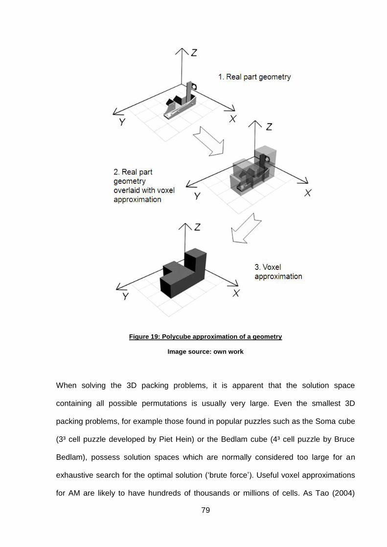
79

Figure 19: Polycube approximation of a geometry

Image source: own work

When solving the 3D packing problems, it is apparent that the solution space

containing all possible permutations is usually very large. Even the smallest 3D

packing problems, for example those found in popular puzzles such as the Soma cube

(3³ cell puzzle developed by Piet Hein) or the Bedlam cube (4³ cell puzzle by Bruce

Bedlam), possess solution spaces which are normally considered too large for an

exhaustive search for the optimal solution („brute force‟). Useful voxel approximations

for AM are likely to have hundreds of thousands or millions of cells. As Tao (2004)

80

notes, such problems can be classed in terms of problem instance size; the larger the

problem instance size, the greater the computational resources required to approach

the problem.

It is safe to state that virtually all AM build volume packing problems belong to the

class of „NP-hard‟ or „intractable‟ problems. For NP-hard (non-deterministic

polynomial-time hard) problems, Tao remarks that there is “no hope to come up with

efficient algorithms to solve them for practical problem instances”. This means that

searching for the globally optimal solution for AM workspace packing is extremely

unlikely to be successful – the goal of the combinatorial optimisation problem is thus to

find an optimised, rather than optimal, solution.

2.4 Summary of the literature review

This chapter on the available background and focal literature has shown that the

subject of AM technology adoption and efficient AM technology usage is treated in a

variety of disciplines.

The notion that geometric complexity is available in AM without an extra monetary

cost has received attention in the literature (Hague et al., 2003). With respect to

energy inputs, classed in this research as a further aspect of AM process economics,

it is interesting to assess if increased shape complexity results in increased process

energy consumption. This investigation contributes to research objective I.

The second of the dual advantages of AM pointed out by Tuck et al. (2008) is treated

in the background literature review. AM‟s role as an investment good enabling the

efficient production of highly differentiated, or customised, products is put into the

context of an economic model by Wong et al. (2008). Further, this review has applied

concepts from technology diffusion and durable goods theory. It is shown that

81

decisions involving technology diffusion, for example the break even process selection

technique (as presented by Ruffo et al., 2006b), can be interpreted as the result of

optimisation behaviour.

The literature review has also presented an overview of the available work on AM

build time, energy consumption, cost, and build volume packing. For this thesis, the

empirical data are collected using a standardised measurement methodology featuring

the construction of a specifically designed test part on different platforms, as done by

Mognol et al. (2006). This results in a unique set of reliable multi-platform summary

data on AM productivity and energy consumption, thereby addressing research

objective II.

The review of the available literature on AM financial cost has revealed a significant

contradiction: while the model by Hopkinson and Dickens (2003) bases estimates on

fully utilised machine capacity, the model by Ruffo et al. (2006b) implicitly assumes

that cost/quantity relationships are valid if machine capacity is not fully used. With

respect to the possibilities afforded by AM, it is unlikely that models constructed by

deliberately leaving capacity unused satisfy the requirement for cost models to

describe configurations of „technical efficiency‟ (as defined by Else and Curwen,

1990). Analogous to models of financial production cost, the parallel character of AM

poses the same set of problems for studies of AM energy inputs. This has been

acknowledged previously by Telenko and Seepersad (2010).

Therefore, a novel combined estimator of AM build time, energy consumption and cost

is required to meet research objective III. It should also incorporate information on the

geometry of the estimated parts.

One further result that can be distilled from this review is that the use of actual 3D data

promotes accuracy of models and algorithms in this context. According to Giannatsis

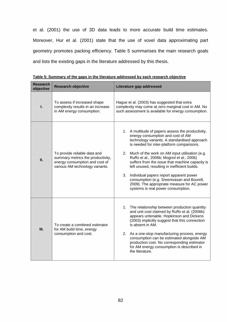
82

et al. (2001) the use of 3D data leads to more accurate build time estimates.

Moreover, Hur et al. (2001) state that the use of voxel data approximating part

geometry promotes packing efficiency. Table 5 summarises the main research goals

and lists the existing gaps in the literature addressed by this thesis.

Table 5: Summary of the gaps in the literature addressed by each research objective

Research objective

Research objective Literature gap addressed

I. To assess if increased shape complexity results in an increase in AM energy consumption.

Hague et al. (2003) has suggested that extra complexity may come at zero marginal cost in AM. No such assessment is available for energy consumption.

II.

To provide reliable data and summary metrics the productivity, energy consumption and cost of various AM technology variants.

1. A multitude of papers assess the productivity, energy consumption and cost of AM technology variants. A standardised approach is needed for inter-platform comparisons.

2. Much of the work on AM input utilisation (e.g. Ruffo et al., 2006b; Mognol et al., 2006) suffers from the issue that machine capacity is left unused, resulting in inefficient builds.

3. Individual papers report apparent power consumption (e.g. Sreenivasan and Bourell, 2009). The appropriate measure for AC power systems is real power consumption.

III. To create a combined estimator for AM build time, energy consumption and cost.

1. The relationship between production quantity and unit cost claimed by Ruffo et al. (2006b) appears untenable. Hopkinson and Dickens (2003) implicitly suggest that this connection is absent in AM.

2. As a one-stop manufacturing process, energy consumption can be estimated alongside AM production cost. No corresponding estimator for AM energy consumption is described in the literature.

83

Chapter 3: Methodology

Chapter 3 discusses the execution of the research leading up to this thesis.

Throughout this work, the overarching goal is to establish and interpret patterns in the

data on part shape, product features, build time, energy consumption and cost,

thereby winning insight into economic implications of AM.

The order in which particular topics are addressed is described in the introduction. As

in the literature review, the material presented in this chapter is divided into separate

sections on the benefits and costs of AM, including energy usage. The various

techniques are discussed, providing an overview of the encountered problems,

solutions to these problems, measurement hardware and used software packages.

The chosen approach to numerical problems is the design of customised algorithms.

Due limited availability of time, funds and coding skill, an emphasis was placed on the

development of pragmatic implementations, often relying on computational power and

simple designs rather than sophisticated concepts and elaborate experimental setup.

3.1 Methodology overview

The successful development of a model that is able to accurately describe the

determinants of AM monetary costs would promote the understanding of the

economics of AM greatly. As argued in the introduction, the economics of a particular

subject are determined jointly by the attached benefits and costs.

Ruffo et al. (2006b) note that the use of AM as a parallel manufacturing technology is

characterised by the simultaneous production of multiple components. The existing

costing models have been constructed on the basis that the degree of AM capacity

utilisation directly impacts process efficiency. This may, however, conflict with the

84

concept of technical efficiency. The incorporation of this principle into novel models of

AM energy consumption and cost is an underlying theme throughout this thesis.

As indicated in the introduction, this analysis treats energy consumption as the most

important proxy of the social cost arising from the operation of electricity-driven

manufacturing technology. Therefore, energy consumption is discussed alongside

monetary cost in this analysis of economic aspects. This forms a simplification, other

aspects of the AM process also lead to an environmental footprint, for example N2

usage or aerosol emissions (Kellens et al., 2011a).

The reason for not expressing the social cost of AM operation in indicator form, for

example through an environmental impact indicator (Kellens et al., 2011a), or even

combining it with monetary cost into an overall private cost indicator, is that the

construction of a credible estimator of this type far exceeds the scope of this thesis.

3.1.1 Software used

This section provides a brief overview of the various software resources employed

over the course of this project. The custom algorithms designed for this research were

written in the statically typed general purpose language C++ as console applications,

using the integrated development environment Dev-C++ (version 4.9.9.2).

This environment is available under the GNU general public license and is hence free

of charge. This setup was chosen because of its open, non-commercial nature, and to

maintain full application portability. By not calling any operating system specific

functions, the resulting implementations are suitable for most operating systems.

Another important reason for selecting C++ instead of MATLAB is that C++ features a

row-major order for the storage of multidimensional arrays in linear memory. As the

implementations operate mainly by manipulating 3D arrays containing voxel

85

approximations of part geometry, the ability to manually code such spatial information

in an intuitive way was of importance. As opposed to the row-major order of C++,

MATLAB features a column-major order of storing information in ≥ 2D arrays, making

the code less accessible. This may, however, be a very subjective criterion.

This thesis does not contain the source code of the developed console applications; it

does however attempt to present the designed algorithms in terms of more legible

pseudo-code in the appendices. All source code is available from the author on

request.

All test geometries were either designed or adapted with the 3D design package

Autodesk 3DS MAX (version 6.0), which is able to assess part geometry for suitability

for the AM processes and to export the correct file format (*.stl). Moreover, where test

geometries were subject to discretisation process (for use in the C++

implementations) this was also carried out manually using 3DS MAX.

The summary data, such as dimensions and volume, for all used test parts (in the *.stl

format) were obtained with the rapid prototyping package Materialise Magics (version

14). Where necessary, this suite was also used for error correction of test part

geometry.

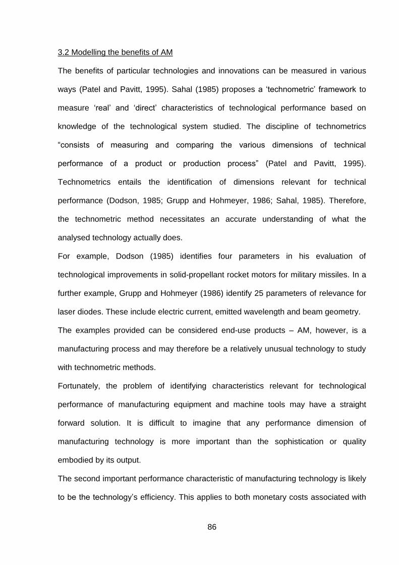
86

3.2 Modelling the benefits of AM

The benefits of particular technologies and innovations can be measured in various

ways (Patel and Pavitt, 1995). Sahal (1985) proposes a „technometric‟ framework to

measure „real‟ and „direct‟ characteristics of technological performance based on

knowledge of the technological system studied. The discipline of technometrics

“consists of measuring and comparing the various dimensions of technical

performance of a product or production process” (Patel and Pavitt, 1995).

Technometrics entails the identification of dimensions relevant for technical

performance (Dodson, 1985; Grupp and Hohmeyer, 1986; Sahal, 1985). Therefore,

the technometric method necessitates an accurate understanding of what the

analysed technology actually does.

For example, Dodson (1985) identifies four parameters in his evaluation of

technological improvements in solid-propellant rocket motors for military missiles. In a

further example, Grupp and Hohmeyer (1986) identify 25 parameters of relevance for

laser diodes. These include electric current, emitted wavelength and beam geometry.

The examples provided can be considered end-use products – AM, however, is a

manufacturing process and may therefore be a relatively unusual technology to study

with technometric methods.

Fortunately, the problem of identifying characteristics relevant for technological

performance of manufacturing equipment and machine tools may have a straight

forward solution. It is difficult to imagine that any performance dimension of

manufacturing technology is more important than the sophistication or quality

embodied by its output.

The second important performance characteristic of manufacturing technology is likely

to be the technology‟s efficiency. This applies to both monetary costs associated with

87

the technology and the consumption of other resources, resulting for example in

unwanted external by-products such as pollution.

As argued in section 2.2.1, measures of the sophistication of manufacturing processes

producing durable goods should reflect benefits or costs arising to the end-user of the

products. To illustrate: if a manufacturing process innovation allows the construction of

more fuel efficient vehicles through light-weighting, the manufacturing technology

features that enable these efficiency gains in the product should be reflected in the

performance dimensions against which the manufacturing technology is evaluated.

This thesis proposes an approach that is suitable for the measurement of „shape

complexity‟ of AM products, which includes aspects of topological and geometric

complexity. This allows research objective I to be addressed. To narrow the scope of

this thesis, the analysis of the impact of shape complexity is restricted to energy inputs

and only performed for the EBM platform.

3.2.1 Quantification of shape complexity

The notion that complexity of geometry may be available in AM at no extra cost

(Hague et al. 2003) sets AM apart from many traditional manufacturing processes.

This may be especially relevant in the context of the economics of AM, as the ability to

efficiently create complex geometries may lead to sophisticated components.

As presented in section 2.2.3.1, the methodology developed by Psarra and Grajewski

(2001), hinging on the measurement of convexity in a geometry, appears suitable for

the quantification of shape features associated with the complexity of 2D shapes. This

approach is able to capture aspects associated with both topological and geometrical

complexity.

88

In this research, the technique proposed by Psarra and Grajewski is transferred to the

analysis of 3D solid geometry. However, the layer-by-layer operating principle of AM

allows the underlying 2D method to be maintained. This is possible because current

additive equipment operates in a strictly sequential manner in which each horizontal

layer is completed before the next layer is deposited onto the existing geometry. Thus,

AM permits a separate analysis of every 2D cross section in the method proposed by

Psarra and Grajewski.

This research adds an additional layer of analysis to the method proposed by Psarra

and Grajewski by subjecting the cross section of test parts to a controlled variation

along the test part‟s Z-axis. Effectively, a continuous 3D solid is split into a set of 2D

layers, so that the level of shape complexity can be varied within one build. The effect

of a variation of shape complexity on process efficiency of AM can then be assessed.

To implement this approach, two preliminary steps are necessary. Initially, a power

monitoring test part (featuring a suitable variation of geometry along its vertical axis) is

defined, as shown in Figure 20.

Figure 20: Standardised power monitoring geometry

Image source: own work

To complement the study of the effect of shape complexity on the deposition of each

layer, the resulting part geometry also features a controlled variation of cross sectional

area, allowing an analysis of the effect of part size.

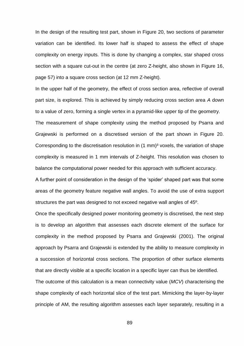
89

In the design of the resulting test part, shown in Figure 20, two sections of parameter

variation can be identified. Its lower half is shaped to assess the effect of shape

complexity on energy inputs. This is done by changing a complex, star shaped cross

section with a square cut-out in the centre (at zero Z-height, also shown in Figure 16,

page 57) into a square cross section (at 12 mm Z-height).

In the upper half of the geometry, the effect of cross section area, reflective of overall

part size, is explored. This is achieved by simply reducing cross section area A down

to a value of zero, forming a single vertex in a pyramid-like upper tip of the geometry.

The measurement of shape complexity using the method proposed by Psarra and

Grajewski is performed on a discretised version of the part shown in Figure 20.

Corresponding to the discretisation resolution in (1 mm)³ voxels, the variation of shape

complexity is measured in 1 mm intervals of Z-height. This resolution was chosen to

balance the computational power needed for this approach with sufficient accuracy.

A further point of consideration in the design of the „spider‟ shaped part was that some

areas of the geometry feature negative wall angles. To avoid the use of extra support

structures the part was designed to not exceed negative wall angles of 45º.

Once the specifically designed power monitoring geometry is discretised, the next step

is to develop an algorithm that assesses each discrete element of the surface for

complexity in the method proposed by Psarra and Grajewski (2001). The original

approach by Psarra and Grajewski is extended by the ability to measure complexity in

a succession of horizontal cross sections. The proportion of other surface elements

that are directly visible at a specific location in a specific layer can thus be identified.

The outcome of this calculation is a mean connectivity value (MCV) characterising the

shape complexity of each horizontal slice of the test part. Mimicking the layer-by-layer

principle of AM, the resulting algorithm assesses each layer separately, resulting in a

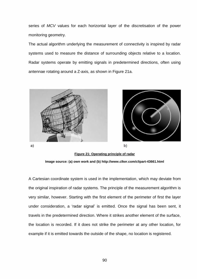
90

series of MCV values for each horizontal layer of the discretisation of the power

monitoring geometry.

The actual algorithm underlying the measurement of connectivity is inspired by radar

systems used to measure the distance of surrounding objects relative to a location.

Radar systems operate by emitting signals in predetermined directions, often using

antennae rotating around a Z-axis, as shown in Figure 21a.

Figure 21: Operating principle of radar

Image source: (a) own work and (b) http://www.clker.com/clipart-43661.html

A Cartesian coordinate system is used in the implementation, which may deviate from

the original inspiration of radar systems. The principle of the measurement algorithm is

very similar, however. Starting with the first element of the perimeter of first the layer

under consideration, a „radar signal‟ is emitted. Once the signal has been sent, it

travels in the predetermined direction. Where it strikes another element of the surface,

the location is recorded. If it does not strike the perimeter at any other location, for

example if it is emitted towards the outside of the shape, no location is registered.

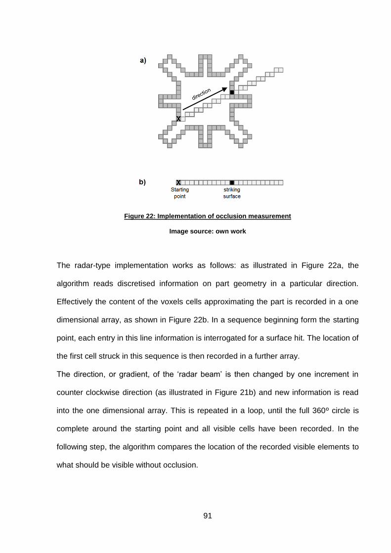
91

Figure 22: Implementation of occlusion measurement

Image source: own work

The radar-type implementation works as follows: as illustrated in Figure 22a, the

algorithm reads discretised information on part geometry in a particular direction.

Effectively the content of the voxels cells approximating the part is recorded in a one

dimensional array, as shown in Figure 22b. In a sequence beginning form the starting

point, each entry in this line information is interrogated for a surface hit. The location of

the first cell struck in this sequence is then recorded in a further array.

The direction, or gradient, of the „radar beam‟ is then changed by one increment in

counter clockwise direction (as illustrated in Figure 21b) and new information is read

into the one dimensional array. This is repeated in a loop, until the full 360º circle is

complete around the starting point and all visible cells have been recorded. In the

following step, the algorithm compares the location of the recorded visible elements to

what should be visible without occlusion.

92

If every existing surface element is visible, the shape is deemed fully convex, as

proposed by Psarra and Grajewski (2001). For intermediate results a value of

connectivity CV ∈ ]0,1] is recorded. This procedure is repeated for all „n‟ elements of

the perimeter in layer „i‟, enabling the calculation of the mean connectivity value MCVi

for each layer, where:

∑

(Eq. 10)

MCV is calculated for all layers in the discretised approximation of the test part.

Effectively, MCVi reflects shape complexity present in the „i‟th horizontal cross section

if the part and thus forms a measure of two dimensional complexity.

It would have been possible to expand this implementation to three dimensions by

measuring the occlusion characteristics of all surface voxels in three dimensions and

thereby arriving directly at a three dimensional metric of shape complexity. However, it

was decided to keep the two dimensional specification. This decision was made as the

underlying additive techniques create each layer in a two dimensional deposition

process. By measuring the complexity of the shape in a succession of horizontal cross

sections of the part, quantitative data is generated on how the complexity of the

geometry varies along the test part‟s Z-axis. Effectively, what has been added to the

methodology used by Psarra and Grajewski by this thesis is the „radar‟ measurement

idea and functionality assessing the shape complexity in a sequence of layers.

To evaluate the logical flow of program code, Overland (2005) suggests writing

„pseudo-code‟, expressing the flow and logical structure of the actions performed by

the program in plain English. The pseudo-code for the complexity measurement

algorithm developed for this project is presented in Appendix B. The code was

93

designed specifically for this research, no parts of code were adapted or taken over

from Psarra and Grajewski (2001).

3.3 Assessing the input usage of AM

After presenting the methodology used to assess AM‟s ability to generate complex

and hence functional products in terms of shape complexity, this section discusses the

measurement of monetary costs and energy consumption associated with the

technology‟s application.

As machine productivity is a critical determinant for both machine energy consumption

and manufacturing cost, its measurement is discussed separately. The single-step

nature of the AM process may afford a new level of clarity in the production of complex

end-use components, as suggested in the introduction. To be able to exploit the

transparency offered by the single-step nature of AM, this thesis pursues the goal of

constructing a novel tool for the combined analysis of the monetary and electricity

inputs.

In response to the technology‟s current shortcomings in terms of dimensional

accuracy and surface finish, AM products are often subject to ancillary post-

processing operations. Routine post processing techniques for metallic AM products

are light finish machining (Cormier et al., 2004) and shot blasting (Mazzioli et al.,

2009). To simplify the arguments brought forward in this thesis, such post-processing

is also ignored in most cases. Where the use of ancillary equipment or processes is

mandatory, this is included in the considerations and clearly stated.

94

3.3.1 Measuring build time

The measurement of build time during the various build experiments is

straightforward. During production, machine activity can normally be differentiated into

multiple states: build atmosphere / vacuum generation, system warm up, material

deposition / exposure, fresh layer deposition, delays during build activity, and system

cool down. However, not all AM technology variants require each step: for example,

FDM does not require an exposure procedure after the deposition of material. The

presence of process elements of particular AM technology variants is discussed in

chapter 5.

Four different approaches were available to record total build time and the duration of

the various phases of machine activity:

1. Interrogation of build reports generated autonomously by the AM

platforms‟ control systems.

2. Analysis of log files compiled by the machine operating systems,

with or without proprietary analysis software from the system

manufacturer.

3. Analysis of energy consumption data with respect to machine

activity. All build experiments were monitored using power

monitoring equipment, therefore a full set of time consumption data

were collected alongside energy consumption data. This approach

was the preferred method and source of data in this thesis.

4. Manual recording of machine activity by the researcher.

95

3.3.2 Power monitoring experiments

To generate the experimental data informing this research, three separate series of

experiments were performed. The first series studies the construction of standardised

power monitoring test parts on a wide range of both metallic and polymeric AM

systems. For each surveyed AM platform, two builds were conducted. In the first

experiment, the energy inputs were monitored during the production of one test part

located in the centre of the build volume floor, as shown in Figure 23a. The second

experiment on each AM platform assessed the energy consumption during AM

operation at full capacity. For these builds, the available build space was populated

with as many instances of the power monitoring geometry as possible. One such

configuration is shown in Figure 23b.

Figure 23: (a) Single part and (b) full build experiments

Source: own work

The preferred method for the determination of the packing configuration is the use of

the build volume packing algorithm developed during this project. However, due to

problems of algorithm performance on the smaller AM systems (especially those

96

requiring every part to be attached to a substrate), the packing configuration for the full

build experiments on the metallic AM systems were determined manually. These

issues are further discussed in the results section. Table 6 summarises the additive

systems, materials and layer thicknesses in the experiments performed in the first

series. Furthermore, the table gives an indication of the time resolution used in

measurements. To help the reader navigate the experimental data, Table 6 also

assigns identification codes to each experiment (A01 to A12). These codes are

applied throughout this thesis.

Table 6: Power monitored builds conducted in the first series (A01 to A12)

Tech. variant

Machine type

Manufacturer reference

Material specification

Layer thickness

Time res. Descr. ID

Laser-based metallic AM

AM250 Renishaw (2011)

Stainless steel 316L

50 µm 1 s

Single part

A01

Full build

A02

M3 Linear Concept Laser GmbH (2011)

Stainless steel 316L

30 µm 1 s

Single part

A03

Full build

A04

EOSINT M270

EOS GmbH (2011)

Stainless steel 17-4PH

20 µm 1 s

Single part

A05

Full build

A06

EBM A1 Arcam AB (2011)

Titanium alloy, Ti-6Al-4V

70 µm 1 s

Single part

A07

Full build

A08

LS EOSINT P390

EOS GmbH (2011)

Polyamide 12, PA 2200

100 µm 1 s

Single part

A09

Full build

A10

FDM FDM400mc Stratasys (2011)

Polycarbonate 178 µm 1 s

Single part

A11

Full build

A12

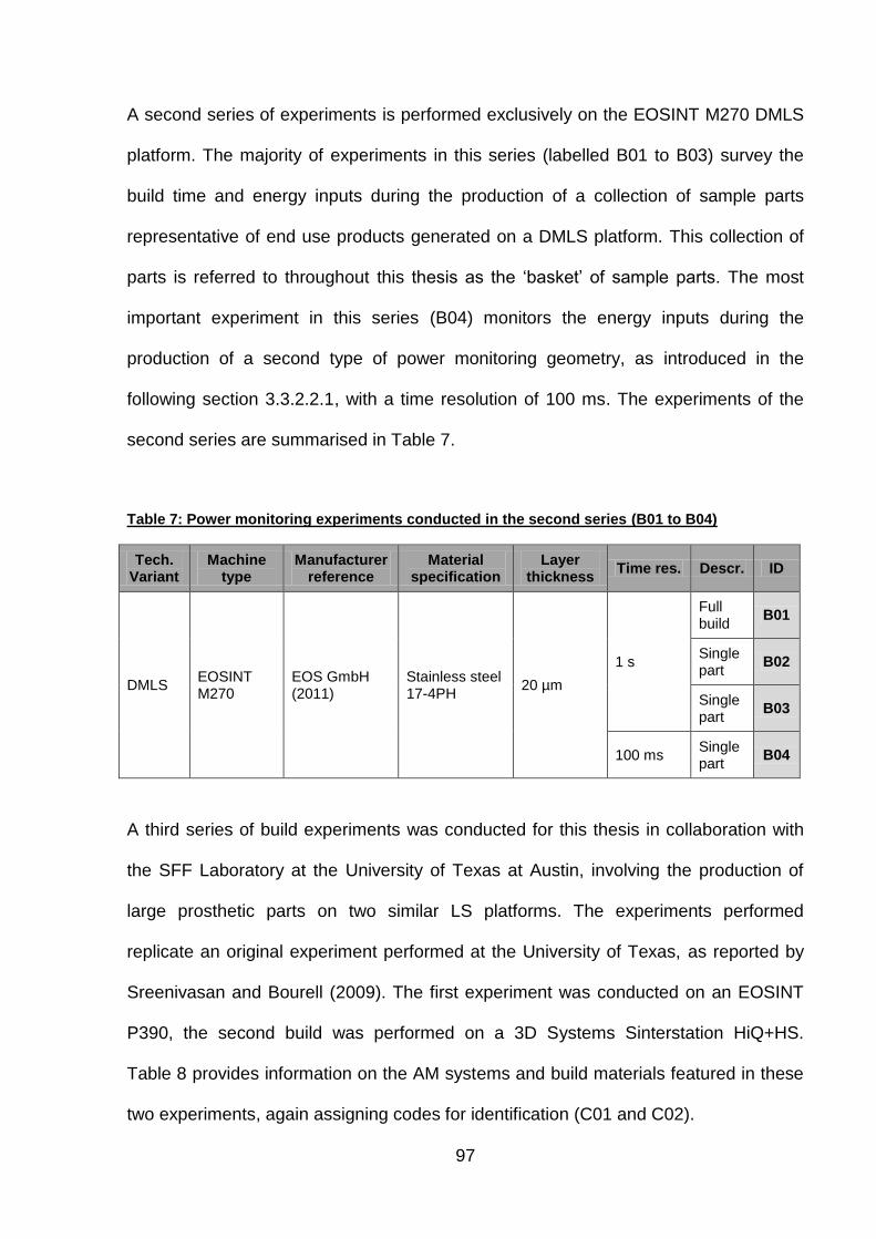
97

A second series of experiments is performed exclusively on the EOSINT M270 DMLS

platform. The majority of experiments in this series (labelled B01 to B03) survey the

build time and energy inputs during the production of a collection of sample parts

representative of end use products generated on a DMLS platform. This collection of

parts is referred to throughout this thesis as the „basket‟ of sample parts. The most

important experiment in this series (B04) monitors the energy inputs during the

production of a second type of power monitoring geometry, as introduced in the

following section 3.3.2.2.1, with a time resolution of 100 ms. The experiments of the

second series are summarised in Table 7.

Table 7: Power monitoring experiments conducted in the second series (B01 to B04)

Tech. Variant

Machine type

Manufacturer reference

Material specification

Layer thickness

Time res. Descr. ID

DMLS EOSINT M270

EOS GmbH (2011)

Stainless steel 17-4PH

20 µm

1 s

Full build

B01

Single part

B02

Single part

B03

100 ms Single part

B04

A third series of build experiments was conducted for this thesis in collaboration with

the SFF Laboratory at the University of Texas at Austin, involving the production of

large prosthetic parts on two similar LS platforms. The experiments performed

replicate an original experiment performed at the University of Texas, as reported by

Sreenivasan and Bourell (2009). The first experiment was conducted on an EOSINT

P390, the second build was performed on a 3D Systems Sinterstation HiQ+HS.

Table 8 provides information on the AM systems and build materials featured in these

two experiments, again assigning codes for identification (C01 and C02).

98

Table 8: Power monitoring experiments conducted in the third series (C01 and C02)

Tech. variant

Machine type

Manufacturer reference

Material specification

Layer thickness

Time res.

Descr. ID

LS

EOSINT P390

EOS GmbH (2011)

Polyamide 12 (PA 2200)

100 µm 1 s Full build

C01

Sinterstation HiQ+HS

3D Systems (2011)

Polyamide 12 (Duraform PA)

100 µm 1 s Full build

C02

3.3.2.1 Power monitoring setup

The energy inputs used by the AM process were measured and recorded using the

Yokogawa CW240 power meter (Yokogawa, 2011). The model CW240 is a digital

power meter that is configurable to various types of power supplies. The meter

employs voltage probes in conjunction with current clamps, as shown in Figure 24.

This enables the calculation of the degree of overlap between the sine curves of

voltage and current and hence allows the determination of the power factor of AC

power supplies.

This is critical for the accurate measurement of real power, which is the determinant of

electric energy consumption. Several studies of AM energy consumption fail to do this,

simply measuring average electric current and multiplying by the nominal voltage of

the connection, for example 240 V. These measurements arrive at results of apparent

power consumption, as opposed to the real power consumption measured with the

CW240.

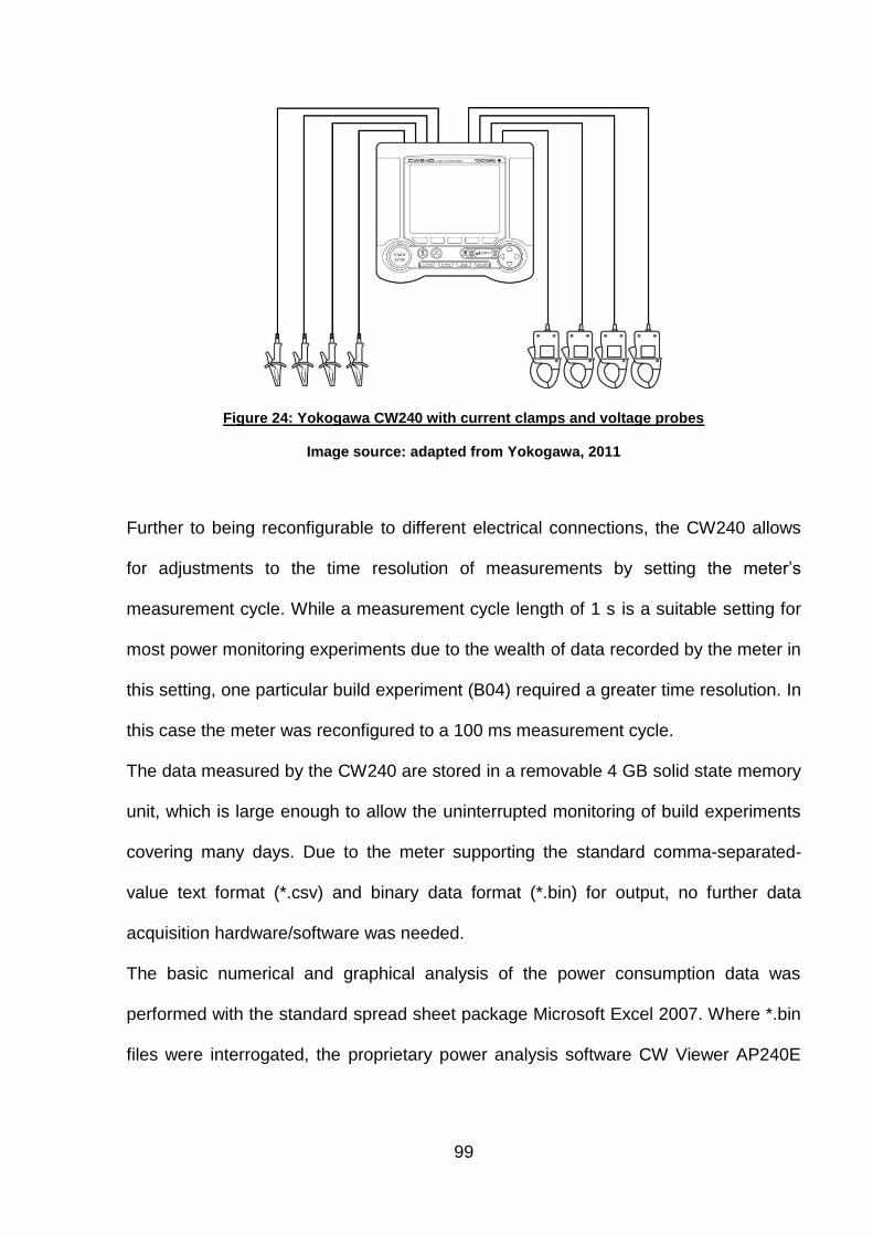
99

Figure 24: Yokogawa CW240 with current clamps and voltage probes

Image source: adapted from Yokogawa, 2011

Further to being reconfigurable to different electrical connections, the CW240 allows

for adjustments to the time resolution of measurements by setting the meter‟s

measurement cycle. While a measurement cycle length of 1 s is a suitable setting for

most power monitoring experiments due to the wealth of data recorded by the meter in

this setting, one particular build experiment (B04) required a greater time resolution. In

this case the meter was reconfigured to a 100 ms measurement cycle.

The data measured by the CW240 are stored in a removable 4 GB solid state memory

unit, which is large enough to allow the uninterrupted monitoring of build experiments

covering many days. Due to the meter supporting the standard comma-separated-

value text format (*.csv) and binary data format (*.bin) for output, no further data

acquisition hardware/software was needed.

The basic numerical and graphical analysis of the power consumption data was

performed with the standard spread sheet package Microsoft Excel 2007. Where *.bin

files were interrogated, the proprietary power analysis software CW Viewer AP240E

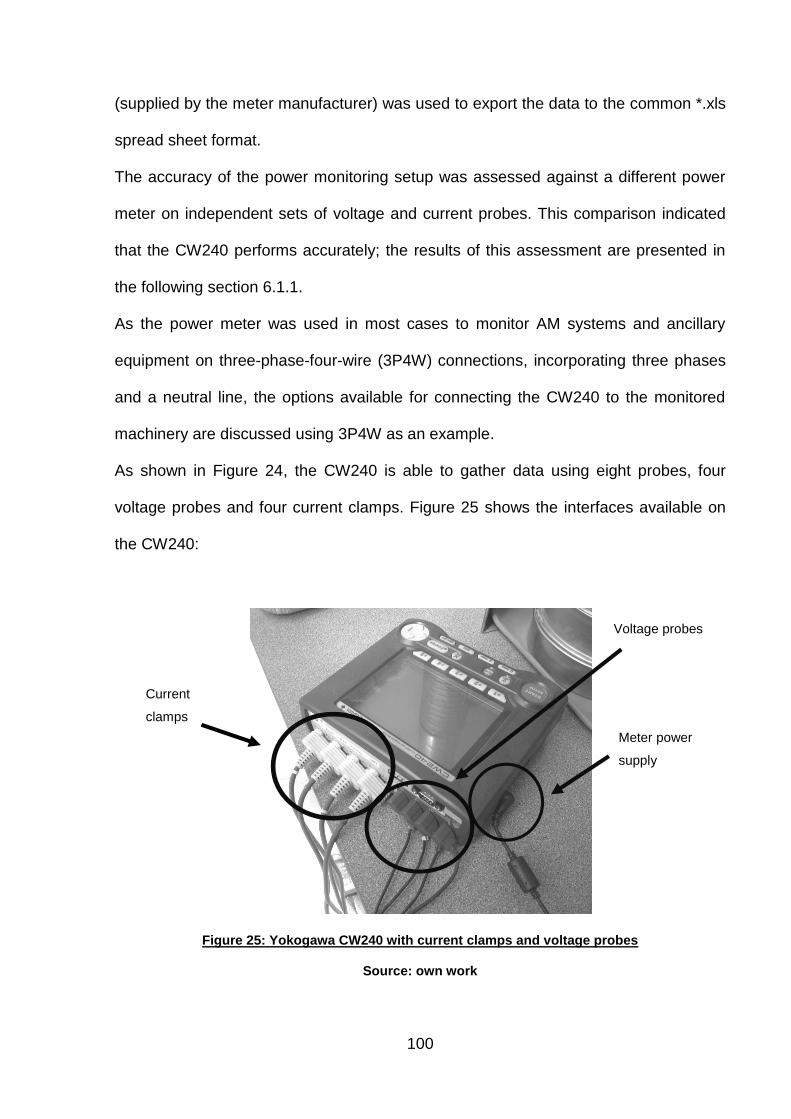
100

(supplied by the meter manufacturer) was used to export the data to the common *.xls

spread sheet format.

The accuracy of the power monitoring setup was assessed against a different power

meter on independent sets of voltage and current probes. This comparison indicated

that the CW240 performs accurately; the results of this assessment are presented in

the following section 6.1.1.

As the power meter was used in most cases to monitor AM systems and ancillary

equipment on three-phase-four-wire (3P4W) connections, incorporating three phases

and a neutral line, the options available for connecting the CW240 to the monitored

machinery are discussed using 3P4W as an example.

As shown in Figure 24, the CW240 is able to gather data using eight probes, four

voltage probes and four current clamps. Figure 25 shows the interfaces available on

the CW240:

Figure 25: Yokogawa CW240 with current clamps and voltage probes

Source: own work

Current

clamps

Voltage probes

Meter power

supply

101

Because the voltage probes need to be in contact with live wires, installing these may

be hazardous. To minimize the risk to the involved technicians and researchers (who

are not trained electricians) the use of fused break-out boxes attached to IEC 60309

16A 400V 3P+N+E(6h) connectors was the preferred method of installing the meter. A

breakout assembly is shown in Figure 26.

Figure 26: Break out boxes, adapters and voltage probes

Source: own work

However, using break out assemblies is only feasible where the AM machinery is

connected to multi-phase power sockets. Where the machinery was connected

permanently to the facility‟s power supply, it was necessary to either improvise wire

break outs or to connect the voltage probes and current clamps internally, as shown in

Figure 27. In several experiments, the power meter was placed inside the AM

machinery to minimise electrical hazard.

Fused

break out

box with

voltage

probes

Current

clamp break

out box

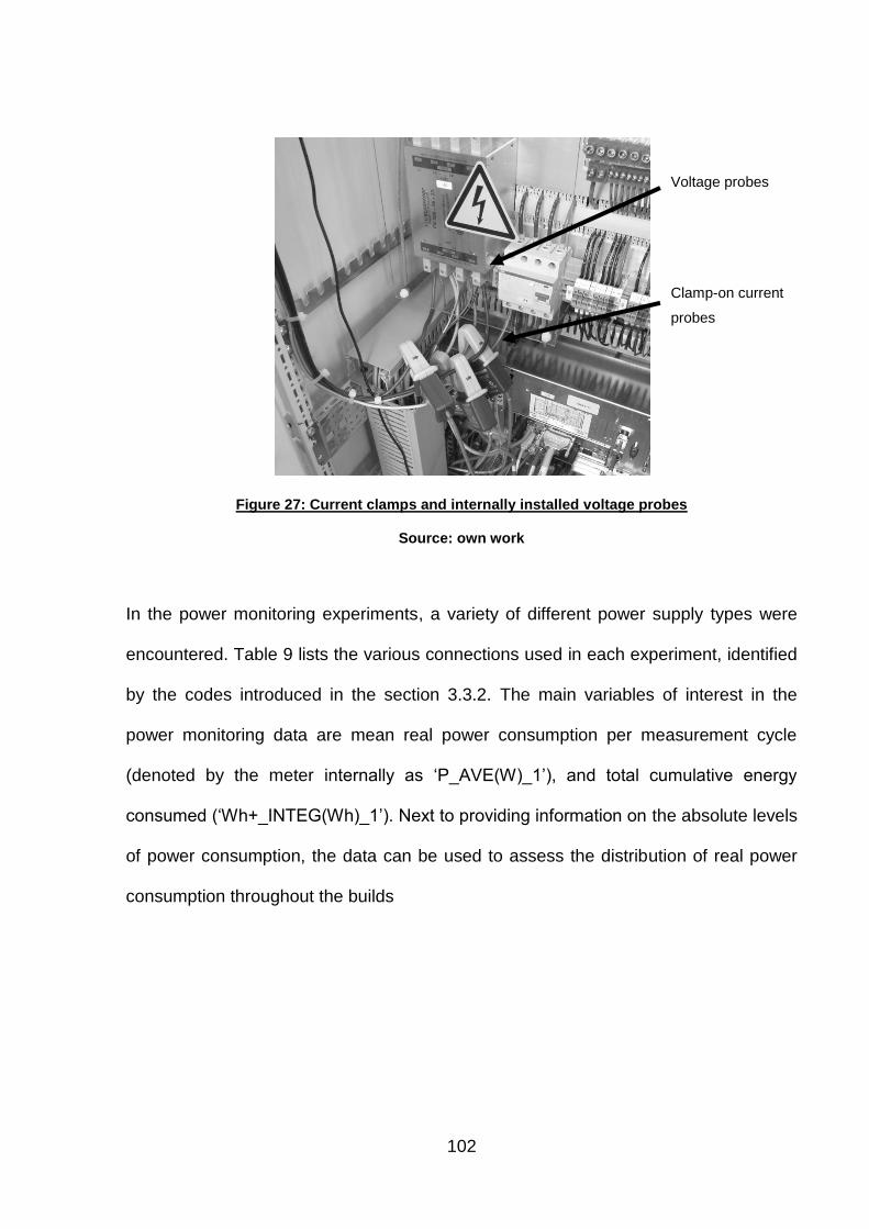
102

Figure 27: Current clamps and internally installed voltage probes

Source: own work

In the power monitoring experiments, a variety of different power supply types were

encountered. Table 9 lists the various connections used in each experiment, identified

by the codes introduced in the section 3.3.2. The main variables of interest in the

power monitoring data are mean real power consumption per measurement cycle

(denoted by the meter internally as „P_AVE(W)_1‟), and total cumulative energy

consumed („Wh+_INTEG(Wh)_1‟). Next to providing information on the absolute levels

of power consumption, the data can be used to assess the distribution of real power

consumption throughout the builds

Voltage probes

Clamp-on current

probes

103

Table 9: Connection types in power monitoring experiments

Technology variant AM system type Connection ID

SLM AM250, Renishaw Single phase A01

SLM AM250, Renishaw Single phase A02

LaserCusing M3 Linear, Concept Laser Three-phase-four-wire A03

LaserCusing M3Linear, Concept Laser Three-phase-four-wire A04

DMLS EOSINT M270, EOS Three-phase-four-wire A05

DMLS EOSINT M270, EOS Three-phase-four-wire A06

EBM A1, Arcam Three-phase-four-wire A07

EBM A1, Arcam Three-phase-four-wire A08

LS EOSINT P390, EOS Three-phase-four-wire A09

LS EOSINT P390, EOS Three-phase-four-wire A10

FDM FDM400mc, Stratasys Three-phase-four-wire A11

FDM FDM400mc, Stratasys Three-phase-four-wire A12

DMLS EOSINT M270, EOS Three-phase-four-wire B01

DMLS EOSINT M270, EOS Three-phase-four-wire B02

DMLS EOSINT M270, EOS Three-phase-four-wire B03

DMLS EOSINT M270, EOS Three-phase-four-wire B04

LS EOSINT P390, EOS Three-phase-four-wire C01

LS Sinterstation HiQ+HS,

3D Systems Three-phase-three-wire C02

In the ideal case, the power consumption of all machine components and sub-systems

is measured separately, as done by Sreenivasan and Bourell (2009) and Kellens et al.

(2010a). However, it was decided that, due to the large number of different AM

platforms surveyed for this research, taking power measurements of all sub-systems

would not be an option. Therefore, this research limits itself to power measurements

taken from the AM system‟s main power supply.

Some AM platforms require a separate power supply for cooling devices. For

example, the AM250 system utilises an external SMC chiller for its cooling fluid.

104

Where such external devices are essential to machine operation, these have also

been monitored using the CW240 in an appropriate configuration.

3.3.2.2 Use of standardised power monitoring test parts

The operating principles of AM technology variants may manifest themselves in

varying levels of energy consumption where build configurations or part characteristics

are changed. An understanding of the relationships may be won by basing power

monitoring experiments on a standardised power monitoring test part which is used for

experiments on all AM platforms, as done by Mognol et al. (2006).

It was decided early on in the design of this research that whole build volumes of parts

should be considered. This is based on the intuition, as presented in chapter 2, that

the production of a single unit surrounded by excess build volume capacity may not be

reflective of cost and energy efficient technology usage in parallel manufacturing.

Essentially, this research extends the argument made against the approach pursued

by Ruffo et al. (2006b) to energy inputs. Following this, models of energy consumption

may thus lead to excessive results if they are based on empty build volume capacity.

Therefore, to be able to make a valid judgement about any type of AM process

efficiency, the concept of technical efficiency should be maintained.

3.3.2.2.1 A power monitoring test part for detailed data

As proposed in section 3.2.1, the sequential layer-by-layer operating principle of AM

systems provides an opportunity for the development of a test part with added

functionality.

For the combined build time, energy consumption and cost estimator developed for

the EOSINT M270, very detailed data of time consumption and energy usage of

105

various process elements are required. The build experiments based on the test part

(A05 and A06) and the components from the basket of representative parts (B01 to

B03) were not capable of delivering the needed level of detail due to the time

resolution being too low.

To achieve the data resolution necessary to understand the patterns of machine

operation and energy consumption during the deposition of each layer, a time

resolution of 100 ms was used in experiment B04.

However, in datasets with a time resolution of 100 ms, new data points are added in

0.1 s intervals. Builds containing multiple parts or individual parts of intermediate size

can easily last for 10 h. With builds of this duration, the generated datasets will contain

hundreds of thousands or millions of data points, resulting in unwieldy file sizes. To

avoid working with such large datasets, a second type of test part was designed. The

test part has a relatively simple geometry and is very flat, with a maximum Z-height of

2.0 mm, as shown in Figure 28.

Figure 28: Power monitoring test part for detailed data (experiment B04)

Source: own work

106

The part varies geometric complexity along its Z-axis similar to the test part shown in

Figure 20 (page 88). However, the second test part is not designed with a continuous

variation of such parameters. The geometry is changed in four discrete steps in 0.5

mm intervals along the part‟s Z-height. In the lowest section, the part exhibits a star-

like shape with dimensions in the X/Y plane of 110 × 110 mm. This is changed to a

square cross section with a side length of 50 mm at a Z-height of 0.5 mm. The next

square cross section begins at a Z-height of 1.0 mm and has a side length of 25 mm.

The uppermost portion of part geometry again has a square shape, with a side length

of 10 mm. By maintaining cross sectional geometry for a number of layers, this

configuration allows the calculation of mean values for time and energy consumption

during the deposition of layer geometry.

This test part was built in the experiment B04, directly on the substrate plate. Due to

the low Z-height of the part, it could not be harvested from the build plate; it was

sacrificed during a wire erosion process in order to reclaim the plate for subsequent

builds.

It is acknowledged that by building the test part shown in Figure 28 directly on the

build plate, an artificial heat transfer situation is created. Production parts are unlikely

to be as flat and will also normally be connected to the substrate via support

structures. However, this artificial situation is not expected to have an effect on the

obtained data as bed heat is not taken into account by the EOSINT M270‟s control

system.

3.3.3 Constructing a combined voxel-based estimator

Problems of creating optimal packing configurations of objects in space are usually

complex, and (as suggested in section 2.3.4.) virtually any instance of such packing

107

problems can be classed as NP-hard. According to Tao (2004), applying the brute

force method of simply trying all possible permutations is not feasible. It is extremely

unlikely that the globally optimal packing configuration can be found in this way.

Therefore, this research proposes an algorithm based on a heuristic leading to

optimised packing configurations.

As discussed by Christensen and Klarbring (2009), discretisation forms an important

strategy in dealing with optimisation problems. The first step in the design of a build

volume packing algorithm is thus to discretise the available build volume space. It can

be described as a cubic 3D lattice containing „cells‟ taking the values „0‟ or „1‟ (or

alternatively, „full‟ or „empty‟), as illustrated in Figure 29.

Figure 29: Discretised build volume, 7³ cells, shown with a unit cube

Image source: own work

If the inserted objects are discretised correspondingly, the initial problem of packing

complicated irregular and continuous geometries into the workspace is transformed

into a polycube packing problem, perhaps similar to the „Soma cube‟ developed by

108

Piet Hein (Hein, 1934). It should be noted that voxels, like pixels, possess a size

quality. This size governs both the accuracy of the discretised approximation of

geometry as well as the computational requirements for the handling the discussed 3D

problem.

Once the part geometries have been converted into voxel approximations and the

build volume itself has been translated into voxel coordinates (including any rounded

work space corners), the task of finding an efficient packing solution becomes a

problem of combinatorial optimisation.

In terms of energy consumption and cost modelling, the approach presented in this

thesis makes one further important simplification, which it shares with all other models

of AM cost in the literature. By limiting itself to the single machine case of AM, the

usage of an individual machine to cater for multi-part demand is modelled.

While this is reflective of the parallel nature of the AM process, as contended by Ruffo

and Hague (2007), it is noteworthy that, especially in a commercial environment, the

AM user may have several machines at his disposal. These could be machines at the

user‟s plant or machines at other locations, perhaps owned by some external provider

of AM services.

Furthermore, the efficient allocation of parts to the available capacity also has a

temporal dimension. For example, the AM user may be able to diminish average unit

cost by postponing production to a later point in time. As with all durable goods, AM

machines can be viewed as providing a stream of services over a period of time

(Waldman, 2003). More precisely, AM machines can be viewed as providing a stream

of available builds from which the user must choose. For N machines and T available

periods, the user‟s full selection problem can be expressed graphically, as done in

Figure 30.

109

Figure 30: The multi-machine inter-temporal AM production scheduling decision

Image source: own work

Therefore, to find the optimal configuration in the realistic inter-temporal, multi-

machine case, the AM user must find the optimal solution across T available builds on

N machines.

Fortunately, the principles governing the behaviour of rational AM users should be

valid in both the single machine and multi machine case. Because the multi-machine

case adds significantly to model complexity and it is felt that it does not add to the

explanatory „bite‟ of the AM costing and energy consumption model, this thesis

concentrates on the single machine case.

Furthermore, a modelling approach was implemented that allows the inclusion of a

temporal aspect of AM activity into the model without resorting to a multi-period model.

The developed modelling technique is discussed in the following section.

110

3.3.3.1 Implementing a build volume packing algorithm

An inter-temporal production decision by the AM user will in practise usually imply that

total demand for parts somehow exceeds the total machine capacity that is

instantaneously available. This is modelled in this thesis by allowing total demand for

parts to exceed build capacity, thereby reflecting demand extending into the future.

However, to construct a working model based on the possibility of such excess

demand, this concept is combined with the definition of some order of precedence for

the multiple parts demanded. By doing this, a measure of comparative urgency of

demand for individual components is introduced, increasing the model‟s richness.

This precedence order is likely to govern the composition of a build if demand is

greater than capacity, as the inclusion of one part is likely to displace another. Thus,

the precedence order can be used during modelling to influence the type of parts

entering the build.

To accommodate multiple components, an instantaneous demand level measured in

discrete units for each of the k parts is given, resulting in a k element vector dd:

[ ] (Eq. 11)

The temporal aspect is introduced into the model by assigning part precedence to

each of the k parts, resulting in a vector p with k elements, where { ∈

} and :

[ ] (Eq. 12)

111

In the following sections, dd will be referred to as the instantaneous demand profile

and p is named the part precedence vector. The mechanism of p and dd works as

follows: dd defines how many units of each of the parts are needed by the user (and if

they are needed at all). The vector p shows the order in which these units are needed,

the type of part for which the „k‟th entry = 1 is the most urgently needed part. The

algorithm tries to insert as many of these parts as possible into the build volume, until

the „k‟th entry in dd is exhausted. After this, the algorithm moves to the next part, as

defined in the precedence vector p. In this way, the algorithm uses p and dd to

determine the order in which parts are inserted into the build volume. It is also

possible that the available build space is not large enough to hold all the parts listed in

dd.

The next step towards the combined estimator is the implementation of the automated

build volume packing algorithm for integration into an AM cost and input efficiency

model. This involves a decision as to which of the broad classes of packing strategies

from the literature is most suitable. As presented in section 2.3.4, a fundamental

distinction is being made between algorithms that insert parts into the build volume in

a fixed sequence (Nyaluke et al., 1996) and strategies that reconsider placement

order or determine part placement simultaneously (Hur et al., 2001; Wodziak et al.,

1993; Ikonen and Biles, 1997).

The idea of basing an algorithm on an instantaneous demand profile dd and on a part

precedence vector p determined outside of the model suggests a novel way of

perceiving the build volume packing problem. The determination of the packing

sequence can be treated as part of a combined model by integrating the packing

algorithm into a specification of AM cost and resource efficiency.

112

This introduces an aspect of rational economic behaviour into the workspace packing

problem. However, it also adds a temporal dimension to these considerations – both

elements are absent from the approaches proposed in the literature (Nyaluke et al.,

1996; Hur et al., 2001; Wodziak et al., 1993; Ikonen and Biles, 1997). Furthermore, by

finding a configuration for the inserted parts in a sequence, a post-placement 3D

compaction problem can be avoided. In this way the algorithm‟s complexity can be

kept to a minimum.

Treating the part placement sequence as exogenously determined (as part of the AM

user‟s economic behaviour) solves the first half of the problem. What is missing is an

idea for a heuristic useful in the optimised placement of each inserted part, together

with an objective function.

This aspect is connected to the use of a voxel-based packing algorithm in this

research. It is felt that a voxel resolution of (5 mm)³ unit cubes is ideal as this is

sufficient to achieve part nesting while still producing relatively simple voxel

approximations.

3.3.3.1.1 Implementation of a barycentric packing heuristic

To design an effective algorithm that is able to cope with a very wide range of different

geometries and part sizes, an evaluation criterion that promotes dense agglomeration

of parts in space (hence producing a nested arrangement) is needed. To implement

this, the packing algorithm was created by developing a barycentric packing heuristic.

Large objects in space attract each other through gravitational forces. Moreover, such

objects form shared centres of gravity. For example, the Earth and the Moon share a

common gravitational centre, also referred to as a barycentre, as shown in Figure 31.

113

Figure 31: Centre of mass in the earth-moon system

Image source: own work

Analogous to the gravitational forces at work between the earth and the moon, the

proposed workspace packing algorithm is based on the heuristic that after the

insertion of parts, these new parts are attracted to the barycentre of the parts already

contained in the build volume.

More specifically, the algorithm is designed to insert, move and rotate geometries in

the build volume, such that their centres of mass are as close as possible to the joint

centre of mass of the parts already present. Based on the voxel-discretisation of both

the build volume space and the parts, the optimised orientation and placement of each

inserted part is determined by a brute force search method.

The brute force method is an exhaustive search technique that simply tries all possible

permutations of part movement and rotation after the new part is inserted. This is

possible because the build volume is discretised with a relatively low resolution of

(5mm)³ and only the placement of the inserted part is assessed. Therefore, the

algorithm can evaluate all possible configurations of the inserted part (the whole

solution space) in a reasonable amount of time. As described above, the evaluation is

done by measuring the distance between the centre of mass of the inserted part and

114

the combined centre of mass (barycentre) of all previously inserted parts. The

configuration that minimises this distance (out of all possible solutions) is chosen.

Once the part location and orientation are determined, a new collective centre of mass

is formed and the next part, governed by the demand profile dd and part precedence

p, is inserted. As placement and rotation are implemented using the brute force

method, the result of each individual part placement step is a globally optimal

configuration. This method comes at the expense of increased computational

requirements. Furthermore, as the parts‟ insertion sequence is exogenously

determined, the overall packing configuration is not optimal.

Hur et al. (2001) suggest that a viable implementation of this class of packing

algorithms is the „bottom-left‟ (BL) approach. In this technique, the first part in the

packing sequence is placed in the build volume at an arbitrary location, normally the

„bottom left‟ corner of the build volume. In this usage, the term „bottom-left‟ is not to be

taken literally as the encountered packing problem is in 3D. For 3D packing problems

with cuboid build volumes, Hur et al. suggest positioning the first part near the origin.

In the algorithm developed for this research, the BL technique is implemented by

inserting and positioning an initial part, which has been assigned the value „1‟ in the

part precedence vector p, in a way that its centre of mass is as close to the origin as

possible. The distance between the barycentre and the origin is simply measured

using the Euclidian norm (vector length). The build envelope and part completeness

are validated throughout the execution of the algorithm by collision checking.

Following the placement of the first part, a second part is inserted, controlled by the

precedence vector p and the demand vector dd. This part is positioned in the build

volume such that the distance between its own centre of mass and the centre of mass

of the first part is minimised. To perform this, the implementation of the algorithm

115

contains functions of part insertion, collision checking, movement and rotation, which

are used throughout the further placement steps. Part placement of the second part is

finalised by calculating a new combined centre of mass, according to the earth-moon

analogy illustrated in Figure 31 (page 113).

The combined centres of mass are computed by creating an n × 3 matrix M and

entering the X, Y and Z coordinates of the centres of the n voxels approximating the

part geometry already present. The voxel centre coordinates, measured in mm, are

obtained simply by multiplying the position of each voxel by the voxel resolution (5

mm) and subtracting one half of the voxel resolution (2.5 mm). A 3 element vector c,

describing the centre of mass, is obtained by computing the mean of each dimension

contained in M:

[ ∑

∑

∑

]

(Eq. 13)

Following the placement of the second part, a third part is inserted and again

positioned and oriented in a way that minimises the distance between its own centre

of mass and the existing combined centre of mass c. As in the previous step, this is

followed by the calculation of a new combined centre of mass cˈ.

This cycle is iterated until one of two events occurs: either, demand for all parts is

exhausted, and thus all elements of the instantaneous demand profile dd are zero, or

the build volume is full and can not accommodate further parts.

A further reason behind this implementation is the variation in build volume utilisation

procedures existing across the various additive platforms in reality. Many AM

processes are incapable of generating geometry that is not supported or anchored in

some way to a substrate or base plate. This may be due to a requirement to

116

mechanically support overhanging elements of geometry or to dissipate thermal

energy. In the currently available spectrum of AM technology variants, the only

processes allowing 3D packing unconstrained by supports are the polymeric LS

process and AM variants employing print heads, such as 3D printing.

The algorithm presented in this section is designed with this difference in mind. To

reconfigure the algorithm from full 3D packing to the „2.5D‟ configuration found in most

AM systems that require parts to be attached to a substrate, Z-movement can be

deactivated. All other functions remain identical.

Figure 32 summarises the various information inputs to the described implementation.

„Operating mode and constraints‟ refers to the ability to pack geometry in full 3D or

2.5D as well as specific build volume size and shape. Part geometries, or rather voxel

approximations thereof, are included into the implementation by global definition in 3D

arrays of integer type. Further inputs are the instantaneous demand profile dd and the

part precedence vector p.

Figure 32: Information inputs to the algorithm

Source: own work

117

To obtain cost and energy efficiency estimates for a part, it is necessary to include at

least one instance of the component into the build volume. If the „i‟th element of the

instantaneous demand profile, ddi, is ≠ 0, it must be made sure that at least one

instance is present in the build, irrespective of part precedence.

This is done by separating the algorithm in two distinct phases. In the first phase, one

instance of the part with the highest precedence is placed close to the origin,

according the BL technique discussed above. Following this, the algorithm inserts and

positions one instance of each further part i for which ddi ≠ 0.

After one unit of each part (if ddi ≠ 0) is inserted, the first phase of the packing

algorithm ends and the second phase begins. Using the same optimisation criterion,

the algorithm inserts and positions as many parts into the build volume as possible.

However, it does this according to the part precedence vector p. Starting with part i

with the highest precedence (pi > pj) the algorithm inserts geometries of this type. It

inserts instances of this part into the build volume until it cannot fit another instance

into the build volume or the number of placed parts exceeds instantaneous demand

for this part. The algorithm then moves on to the next geometry in the part precedence

vector. This is repeated for all parts according to the precedence vector.

Once the packing algorithm terminates, an output of the packing configuration is

automatically created. Apart from displaying the build volume on screen in a text

based console application, the implementation also includes file output functionality.

This allows the generation of a comma separated value (*.csv) text file, which can

then be processed using a standard spread sheet application, such as Microsoft

Excel. The packing algorithm is shown in pseudo-code form in Appendix C.

As discussed above, the packing algorithm operates by calling four main functions:

part insertion, collision checking, rotation and movement.

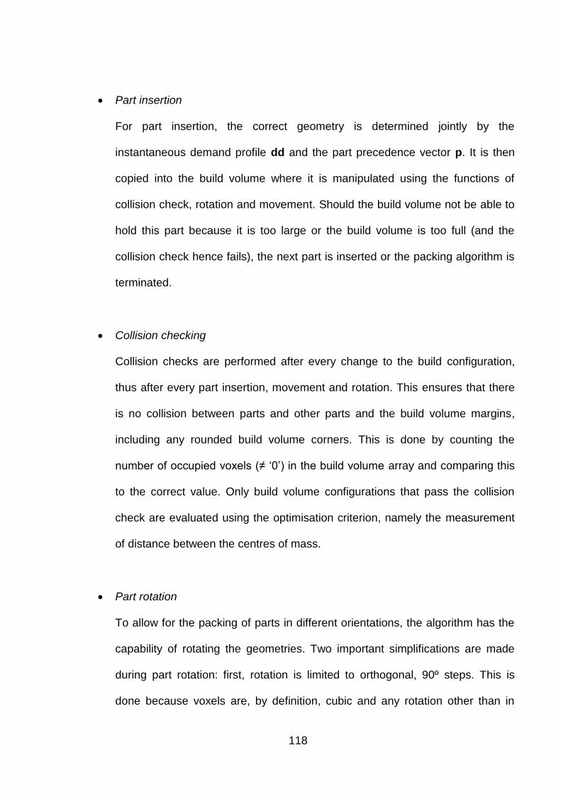
118

Part insertion

For part insertion, the correct geometry is determined jointly by the

instantaneous demand profile dd and the part precedence vector p. It is then

copied into the build volume where it is manipulated using the functions of

collision check, rotation and movement. Should the build volume not be able to

hold this part because it is too large or the build volume is too full (and the

collision check hence fails), the next part is inserted or the packing algorithm is

terminated.

Collision checking

Collision checks are performed after every change to the build configuration,

thus after every part insertion, movement and rotation. This ensures that there

is no collision between parts and other parts and the build volume margins,

including any rounded build volume corners. This is done by counting the

number of occupied voxels (≠ „0‟) in the build volume array and comparing this

to the correct value. Only build volume configurations that pass the collision

check are evaluated using the optimisation criterion, namely the measurement

of distance between the centres of mass.

Part rotation

To allow for the packing of parts in different orientations, the algorithm has the

capability of rotating the geometries. Two important simplifications are made

during part rotation: first, rotation is limited to orthogonal, 90º steps. This is

done because voxels are, by definition, cubic and any rotation other than in

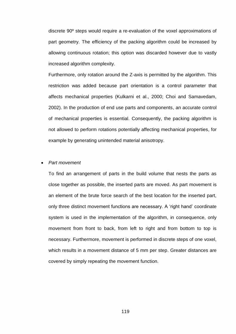
119

discrete 90º steps would require a re-evaluation of the voxel approximations of

part geometry. The efficiency of the packing algorithm could be increased by

allowing continuous rotation; this option was discarded however due to vastly

increased algorithm complexity.

Furthermore, only rotation around the Z-axis is permitted by the algorithm. This

restriction was added because part orientation is a control parameter that

affects mechanical properties (Kulkarni et al., 2000; Choi and Samavedam,

2002). In the production of end use parts and components, an accurate control

of mechanical properties is essential. Consequently, the packing algorithm is

not allowed to perform rotations potentially affecting mechanical properties, for

example by generating unintended material anisotropy.

Part movement

To find an arrangement of parts in the build volume that nests the parts as

close together as possible, the inserted parts are moved. As part movement is

an element of the brute force search of the best location for the inserted part,

only three distinct movement functions are necessary. A „right hand‟ coordinate

system is used in the implementation of the algorithm, in consequence, only

movement from front to back, from left to right and from bottom to top is

necessary. Furthermore, movement is performed in discrete steps of one voxel,

which results in a movement distance of 5 mm per step. Greater distances are

covered by simply repeating the movement function.

120

3.3.3.2 A representative basket of parts

To produce energy and cost estimates that reflect technology usage in practise, a

„basket‟ of representative parts was composed. As the AM system assessed in this

combined study of manufacturing cost and energy consumption generates metal

components (the EOSINT M270 DMLS platform), viable designs for metal

components were chosen. To cover a wide range of applications for metal

components, two fixtures, one mechanical component and two parts with aerodynamic

functionality were chosen.

Once the basket parts were chosen, they were imported into the 3D graphics package

Autodesk 3DS MAX (version 6) for a manual discretisation procedure to obtain the

(5 mm)³ unit cube voxel approximations required by the C++ implementation. This

procedure was carried out by placing the imported *.stl geometry in a container of

voxels. After some minor movement to position the part relative to the voxel

boundaries, the discretised approximation was obtained by deleting all voxels not

containing any part geometry. The precise placement of the parts within their voxel

approximations was also important to ensure that gaps between parts are large

enough if two voxel approximations are located directly next to each other. To ensure

a sufficient distance between parts, no part geometry was allowed within 1 mm of the

vertical boundaries of the voxel approximation.

To accommodate supports and to avoid parts undercutting each other during the build

volume packing process, no overhanging geometry was permitted. This was done by

including all empty voxels beneath geometry in the approximation. Figure 33 illustrates

the discretisation procedure using the example of the power monitoring test part

shown in Figure 20 (page 88).

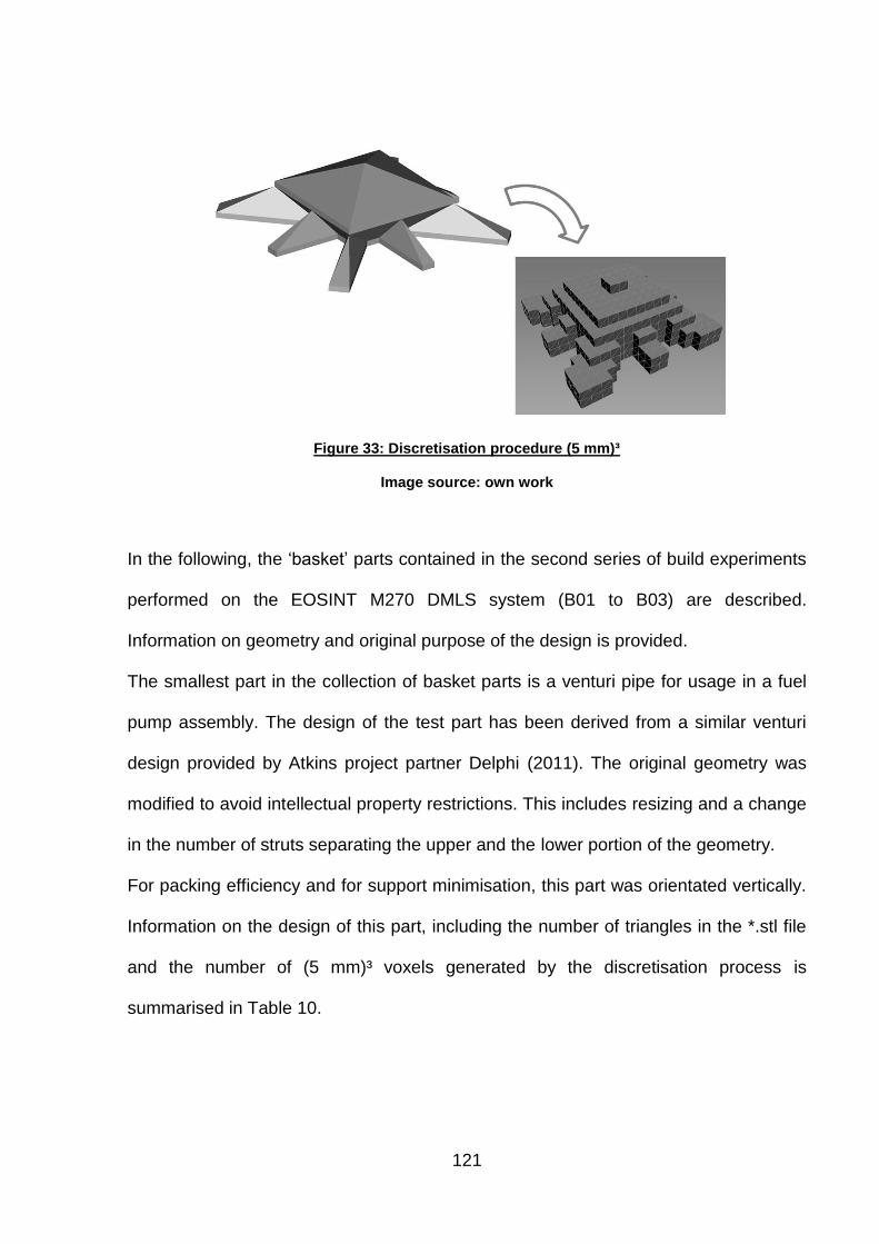
121

Figure 33: Discretisation procedure (5 mm)³

Image source: own work

In the following, the „basket‟ parts contained in the second series of build experiments

performed on the EOSINT M270 DMLS system (B01 to B03) are described.

Information on geometry and original purpose of the design is provided.

The smallest part in the collection of basket parts is a venturi pipe for usage in a fuel

pump assembly. The design of the test part has been derived from a similar venturi

design provided by Atkins project partner Delphi (2011). The original geometry was

modified to avoid intellectual property restrictions. This includes resizing and a change

in the number of struts separating the upper and the lower portion of the geometry.

For packing efficiency and for support minimisation, this part was orientated vertically.

Information on the design of this part, including the number of triangles in the *.stl file

and the number of (5 mm)³ voxels generated by the discretisation process is

summarised in Table 10.

122

Table 10: Venturi pipe

File name venturi.stl :

Height 30.764 mm

Width 9.900 mm

Length 9.902 mm

Triangles in *.stl 59294

Volume 1314 mm³

Surface area 1278 mm²

Number of voxels 28

Image source: own work

The second smallest part included in the basket of representative sample parts is an

end cap for an extrusion profile. This profile forms part of a sliding door assembly. The

*.stl file is adapted from an original design with a manufacturer logo on the part‟s face.

Further, for the adapted version used in this model, the part dimensions are changed

slightly.

Like the above discussed venturi pipe, this is a part that would be demanded in large

numbers. To minimise the requirement for support structures and for easy removal of

supports, the part is oriented with its positioning pins pointing upwards. Summary

information on part details is provided in Table 11.

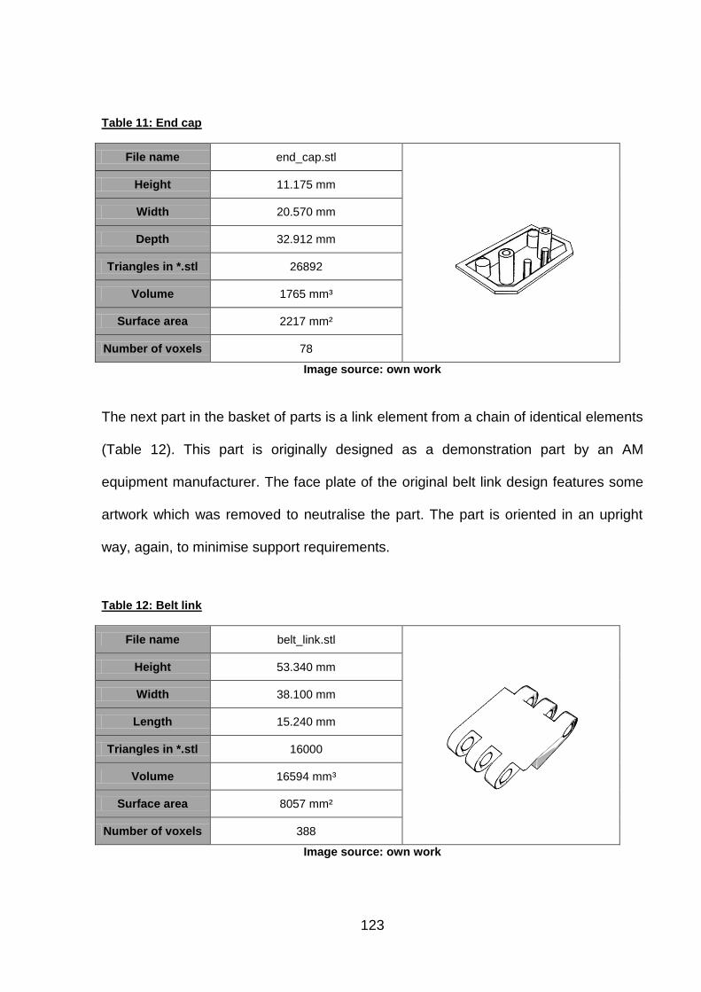
123

Table 11: End cap

File name end_cap.stl

Height 11.175 mm

Width 20.570 mm

Depth 32.912 mm

Triangles in *.stl 26892

Volume 1765 mm³

Surface area 2217 mm²

Number of voxels 78

Image source: own work

The next part in the basket of parts is a link element from a chain of identical elements

(Table 12). This part is originally designed as a demonstration part by an AM

equipment manufacturer. The face plate of the original belt link design features some

artwork which was removed to neutralise the part. The part is oriented in an upright

way, again, to minimise support requirements.

Table 12: Belt link

File name belt_link.stl

Height 53.340 mm

Width 38.100 mm

Length 15.240 mm

Triangles in *.stl 16000

Volume 16594 mm³

Surface area 8057 mm²

Number of voxels 388

Image source: own work

124

The second largest part in the representative basket of parts is a turbine wheel

designed by a graduate student at Loughborough University. In the basket of sample

parts, this design features the largest number of triangles in the *.stl file. In terms of

the file format this may indicate that its geometry is complex or that the resolution of

the file is very high (both is the case). Information on this part is summarised in Table

13.

Table 13: Turbine Wheel

File name turbine_ wheel.stl

Height 28.000 mm

Width 53.999 mm

Length 54.017 mm

Triangles in *.stl 107808

Volume 20618 mm³

Surface area 11625 mm²

Number of voxels

604

Image source: own work

The largest part selected for the basket parts, as measured in part volume and

number of voxels in the discretised approximation, is a bearing block as shown in

Table 14. As the original geometry was very basic, it was modified to incorporate a

greater degree of sophistication of design, including a cut out in its roughly planar

base section.

125

Table 14: Bearing block

File name bearing_block.stl

Height 52.061 mm

Width 76.138 mm

Length: 127.096 mm

Triangles in *.stl 11358

Volume 96645 mm³

Surface area 28953 mm²

Number of voxels 1716

Image source: own work

This chapter recognises that the parts contained in this basket of sample parts were

not all derived from end-use parts (belt link and bearing block) or were not designed

specifically for manufacturing by additive processes (venturi pipe). This may have a

negative effect on the realism of the model. Moreover, it is acknowledged that the

basket represents a convenience sample of parts. This may further limit the realism of

the model by introducing selection bias. In future versions of this methodology, the

basket should be drawn at random from a large sample of designs manufactured in a

commercial setting on the EOSINT M270.

3.3.3.3 Build time estimation

Once an efficient build configuration is determined by the build volume packing

algorithm, the next step is to estimate build time, which forms a prerequisite for cost

estimation (Ruffo et al., 2006b; Munguia, 2009). The estimate for total build time, Tbuild,

is obtained by combining data from a hierarchy of elements of time consumption:

fixed time consumption per build operation TJob, including, for example machine

atmosphere generation and machine warm up,

126

total layer dependent time consumption, obtained by multiplying the fixed time

consumption per layer TLayer by the total number of build layers l,

the total build time needed for the deposition of part geometry approximated by

the voxels. The triple Σ operator in Equation 14 is used to express the

summation of the time needed to process each voxel TVoxel xyz in a 3D array

representing the discretised build configuration.

( ) ∑∑ ∑

(Eq. 14)

No allowance is made for build preparation and machine cleaning. It is felt that the

time spent on these activities is difficult to measure and very much at the discretion of

the machine operator. It could be argued that these activities take place during the

42.96 % of non-operational hours, as cited by Ruffo et al. (2006b).

3.3.3.4 Energy consumption estimation

Total energy investment, EBuild, can be modelled similarly. A purely time dependent

element of power consumption must be expected in the continuous operation of AM

machinery. This is denoted by the energy consumption rate ĖTime, (measured in MJ

per s) which is multiplied by TBuild to estimate total time-dependent energy

consumption.

Modelling ĖTime as a constant reflects its interpretation as a constant base line level of

energy consumption throughout the build, originating from continuously operating

machine components such as cooling fans, pumps and the control system. Analogous

to build time estimation, EJob and ELayer denote fixed elements of energy consumption

127

per build and layer, for a total number of layers ‘l’. Further, the geometry dependent

energy consumption is obtained by adding all energy consumption associated with

voxel deposition EVoxel xyz throughout the discretised workspace.

( ) ( ) ∑∑ ∑

(Eq. 15)

Both the time and energy estimators possess information on the real Z-height of the

parts contained in the build. This approach is chosen to avoid large estimation errors

arising from the inclusion of empty layers at the top of builds.

It is noteworthy that AM energy consumption also enters the cost model by Ruffo et al.

(2006b), albeit through production overheads. Ruffo et al. express energy

consumption in money terms (1.5 € of energy expenditure per hour of machine

operation) and combine all electricity consumption attributable to the AM facility,

including the machine, auxiliary systems and the building containing the machinery.

While this at first appears to be too crude to be relevant, it does carry an important

message. In the costing model by Ruffo et al., energy consumption is viewed as an

indirect cost and is thus entirely build time dependent. As will be shown in the model

constructed in the following chapter, this is one alternative to typify energy

consumption of AM systems. Energy consumption could have entered the model

constructed by Ruffo et al. (2006b) equally well as a part weight dependent (and

hence geometry dependent) cost.

As in the above, the measurement algorithm underlying the combined estimator of

build time, energy consumption and cost can be expressed in pseudo-code

(Appendix D).

128

3.3.3.5 Production cost estimation

For this research, an activity based cost (ABC) estimator of the type devised by Ruffo

et al. (2006b) is employed. The cost estimate for the build CBuild is constructed by

combining data on the total indirect costs and direct costs incurred, thereby providing

a measure of “relatively well structured” costs (Son, 1991) ignoring costs arising from

risk of failure, setup, waiting, idleness and inventory.

Indirect costs, expressed as a cost rate ĊIndirect measured per machine hour, contain

costs arising from administrative and production overheads, production labour, as well

as machine costs (including depreciation). Table 15 lists the constituents of the used

costing model, most items are adapted from data provided by Ruffo et al. (2006b).

129

Table 15: Direct and indirect cost elements

Cost item Value

Production overhead

Rent, building area cost 4.53 £ / h †

Administration overhead

Hardware purchase 1670.27 £ †

Software purchase 1670.27 £ †

Hardware cost/year 334.05 £ †

Software cost/year 334.05 £ †

Consumables per year 1113.52 £ †

Total administration overhead 0.31 £ / h †

Production labour

Technician annual salary 25165.45 £ †

Employer contributions 22.00 % †

Total production labour 6.14 £ / h †

Utilisation

Utilisation rate 57.04 % †

Annual machine operating hours 5000.00 h †

Equipment

AM equipment and wire eroder 8.00 years †

Hardware and software 5.00 years †

Machine costs

Machine purchase 364406.80 £

Machine purchase cost per year 45550.85 £

Maintenance cost per year 22033.90 £

Machine consumables per year 2542.37 £

Wire erosion machine purchase 55000.00 £

Total wire erosion costs per year 8165.00 £

Total machine costs per year 78292.12 £

Total machine costs 15.66 £ / h

Total indirect cost per machine hour 26.64 £ †

Direct cost for 17-4 PH powder / kg 78.81 £

Direct electricity cost per MJ 0.018 £

†adapted from Ruffo et al. (2006b)

As listed, this research estimates the total indirect cost rate of operating the EOSINT

M270 at £ 26.64 per hour. It is noteworthy that the system incorporates a nitrogen

generator; hence no protective gas from external sources is needed.

130

The data marked with † in Table 15 have been adapted from Ruffo et al. by converting

the currency from € into £ at the 2006 exchange rate (adjusting for inflation).

Unlike Ruffo et al., two direct costs now enter total cost: raw material cost and energy

cost. Total raw material costs are calculated by multiplying the total weight w of all

parts included in the build (including support structures) with the price per kg of the

stainless steel 17-4 PH powder, PRaw Material (£ 78.81 per kg). The expenditure for

energy enters the model by multiplication of the energy consumption estimate EBuild

with the mean price of electricity for the manufacturing sector in the UK, PEnergy,

currently around £ 0.018 per MJ (according to DECC, 2010). Thus, the total cost

estimate for the build CBuild can be expressed as:

( )

(Eq. 16)

3.4 Summary of methods

Adhering to the split structure described in the introduction to this thesis, the

presented methodology deals with the treatment of benefits and costs (also measured

in energy terms) of AM usage separately.

A method aimed at capturing the technology‟s ability to efficiently create complex

products has been presented. This approach is viable for the assessment of shape

complexity of individual layers of geometry. As a novel application of the method

proposed by Psarra and Grajewski (2001), this method is suitable for exploring the

question of whether the shape complexity of part cross sections impacts input

utilisation, contributing to research objective I. This is especially interesting in the

context of energy consumption, as a link between energy consumption and the

131

complexity of products has not received attention in the AM specific literature.

Moreover, a clear connection of this type has been demonstrated for substitute

process technologies, for example CNC machining (Morrow et al. 2007).

The methodology aimed at assessing the cost and energy side of AM usage

concentrates on approaches that are able to accommodate for differences in capacity

utilisation. As elaborated in the summary of the literature review (section 2.4) existing

empirical work on AM energy consumption and cost fails to account for this. Much of

the research effort described in section 3.2 is expended for the generation of empirical

data and models that are able to accommodate the parallel nature of AM technology,

thereby contributing to research objective II.

Section 3.3 further develops the methodology for the construction of a combined

estimator of AM build time energy consumption and cost, addressing research

objective III. Using this model, the true determinants of the efficient operation of AM

technology variants can be investigated.

132

Chapter 4: Results on benefits of AM

This chapter discusses the results of this research relating to the benefits of being

able to economically realise complex products. AM‟s ability to create complex

products can be analysed using a framework aimed at different aspects of shape

complexity.

As demonstrated in section 3.2.1, it is possible to quantify geometric parameters that

are associated with shape complexity by applying a visibility metric. Applied to a

dedicated test part, the result of this quantification is presented in the following

section.

In this thesis, the results of the shape complexity analysis are applied to the Arcam A1

EBM platform. This is done using a correlation analysis of the shape complexity metric

versus energy consumption per layer deposited in the full build experiment, introduced

as experiment A08 in the previous chapter. In an attempt to meet research objective I,

the correlation coefficients are then discussed below in section 7.1.1.

4.1. Results of the shape complexity analysis

The part shown in Figure 20 (page 88) serves as the subject for an assessment of the

energy consumption on various AM platforms. It is tailored for an analysis of the effect

of shape complexity, proxied by the measurement of the attribute of convexity (as

suggested by Psarra and Grajewski, 2001). This is done to address the question of

whether increasing shape complexity comes at additional energy usage in AM,

corresponding to research objective I described in the introduction.

As introduced in section 3.2.1, this is implemented by varying the „occlusion‟

parameter associated with shape complexity along the height of the test parts,

133

effectively changing a complex star shaped cross section into a simple square (fully

convex).

Cross-sectional shape complexity is quantified by calculating a mean measure of

occlusion present in the layer‟s perimeter, using the method proposed by Psarra and

Grajewski. The resulting metric of shape complexity is the mean value of

„connectivity‟, MCVi, for each layer „i‟. As the implementation of the measurement

algorithm is based on a resolution of (1 mm)³ voxels, the corresponding variation of

test part parameters is measured in 1 mm intervals of Z-height.

Figure 34 shows the variation of three parameters along the test part‟s Z-axis: the total

area of the part‟s cross section, the cross-sectional perimeter length and the

parameter of shape complexity proposed by Psarra and Grajewski. For exposition,

MCV is shown in inverted form, such that a high value of MCV-1 indicates high cross-

sectional shape complexity.

Figure 34: Variation of parameters of geometry

Image source: own work

134

As Figure 34 demonstrates, the area of the cross-sections dips between 2 and 12 mm

of Z-height, from an initial value of 1850 mm² to around 1450 mm². This fluctuation

occurs alongside the controlled variation of MCV. The fact that both parameters are

varied in parallel complicates the analysis of the pure effect of a variation of MCV.

However, it does allow the design of a relatively simple polygonal test part without

curved surfaces, as shown in Figure 20 (page 88).

The irregularity in the MCV-1 curve at a Z-height of 6 mm results from the use of a

discretised voxel representation of part geometry. It is thus an artefact of the

discretisation technique and should be ignored.

Figure 34 further demonstrates that the design of a test part varying parameters of

complexity and cross-sectional area is successful. The effect of the designed variation

of area and complexity can be assessed in conjunction with AM process energy

consumption data.

4.2 Applying the shape complexity metric to EBM energy consumption

The question of whether product complexity may be „free‟ in terms of process energy

consumption, as posed by research objective I, is addressed by analysing the data log

files generated by the A1 EBM platform in conjunction with the power monitoring data

collected during the builds and the complexity metric proposed by Psarra and

Grajewski (2001). The data log files, in the proprietary *.plg file format, have been

retrieved from the Arcam A1‟s control computer and interrogated using the proprietary

data analysis tool Log Studio 3 (v.3.1.51). A screenshot of the Log Studio 3 user

interface is located in Appendix E.

Using these data it is possible to divide energy invested during the core build time into

three machine activities, layer preparation, preheating and melting. For the full build

135

experiment (A08, as defined in chapter 3) Figure 35 shows that the energy expended

during layer preparation (data loading and fresh powder deposition) fluctuates around

a constant mean throughout the build (approximately 10 kJ per layer). In contrast, the

energy expended during the preheating state exhibits a linear, slightly negative, trend

– most likely due to a gradual warming up of the machine frame during the build

process. More interestingly, the energy expended for the selective melting of the cross

sections fluctuates strongly. The initial spike in energy consumption (during the first

layer) is explained by repeat melting to ensure full attachment of parts to the build

platform.

Figure 35: EBM energy invested per layer, by activity

Image source: own work

136

Numerically, the effect of the variation of shape complexity in the test parts contained

in the build and the energy consumed during the deposition of each layer can be

analysed using simple Pearson product moment correlation coefficients ρX,Y ,where

, (Eq. 17)

and σXσY is the product of the standard deviations of variables X and Y. This

coefficient expresses the degree of linear dependency between two variables.

A sample correlation coefficient ρAREA,LAYER ENERGY = 0.9699 between selective melting

energy and cross sectional area (in 1 mm intervals of Z-height) suggests that total

melting energy consumption is indeed determined by cross sectional area, and thus

by overall part mass.

Further applying correlation coefficients, the effects of various aspects of geometry on

the energy expended for layer melting can be assessed. Focussing on the portion of

the build containing variation of shape complexity (1-12 mm Z-height, as presented in

Figure 34, page 133), correlation coefficients between layer energy and cross-

sectional perimeter length, complexity and melting area can be compared:

6568.0, ENERGYLAYERPERIMETER (Eq. 18)

8263.0, ENERGYLAYERAREA (Eq. 19)

3544.0, ENERGYLAYERMCV (Eq. 20)

The coefficients demonstrate that melting energy consumption correlates with cross

section area, and to a lesser extent with perimeter length. The correlation coefficient

between layer energy consumption and the used measure of shape complexity

is small and negative (-0.3544).

137

This can be viewed as an indication of a weak or potentially absent association

between EBM energy consumption and shape complexity. It should be noted that the

negative correlation coefficient originates from the formulation of MCVi (a high value

indicates a small degree of shape complexity and vice versa).

The results of this correlation analysis are further discussed in the context of the

platform‟s operating principle in section 7.1.1.

138

Chapter 5: Results on machine productivity and build volume packing

The material deposition speed with which AM systems build up the features of product

geometry is a highly relevant factor for process economics. As observed by Ruffo et

al. (2006b), a large proportion of the financial cost arising during the operation of an

AM system can be attributed to build time. Further, Luo et al. (1999) suggest that build

speed is also a critical determinant of AM process energy consumption.

Chapter 5 presents the experimentally collected data on the productivity of various AM

technology variants researched for this project. Following a short description of each

build experiment (identified using the codes introduced above in section 3.3.2, page

96) the measured material deposition rate is presented for each platform. Distinctions

between time spent for warm up and cool down are made only where the AM

technology variant under consideration employs such process elements and they are

identifiable in the data. The empirical results and summary metrics are presented to

contribute reliable estimates of AM build speed, energy consumption and cost to the

data available in the literature, thereby addressing research objective II. They also

provide the data needed for the construction of the combined estimator, meeting

research objective III.

5.1 Laser-based AM processes utilising a powder bed

As presented in section 3.3.2, three AM platforms belonging to the class of laser-

based metallic powder bed fusion processes have been assessed in this research: the

Renishaw AM250, the ConceptLaser M3 Linear and the EOSINT M270, from EOS

GmbH. Despite sharing the same operating principle and using similar stainless steel

build materials in the experiments, the three platforms exhibit significant differences in

139

terms of machine productivity. This may be due to different layer thickness settings

and laser types.

It should be noted that the power monitoring test parts contained in the experiments

were attached to the build substrate in different ways. On the AM250, dedicated 3 mm

tall support structures were used to attach the components, whereas on the M3 Linear

the first layer is simply repeated multiple times until a Z-height of 1 mm is reached. On

the EOSINT M270, the parts were constructed directly on the substrate.

The different methods for attaching the parts to the build plate have an effect on the

heat transfer between the parts and the substrate. Building the test part (shown in

Figure 20, page 88) directly on the platform maximises heat transfer. Connecting the

parts by extrusion, as done on the M3 Linear, will also lead to good heat transfer. In

contrast, building the parts on supports, as done on the AM250 with material powder

between the support features, limits heat transfer. For energy consumption during the

deposition of the parts, however, the difference in heat transfer is likely to be irrelevant

as these platforms (unlike EBM systems) do not measure powder bed temperature to

control the build process. Thus, the observed energy consumption and machine

productivity (beyond the deposition of the support structures) should not be impacted

by the method of attaching the test parts to the build plate.

Further, it should be remarked that the AM250 system used in the build experiments

was not a final specification machine. This led to some problems with laser focus

position during the experiments, diminishing the applicability of the results obtained for

this particular platform.

The full build experiments on the three platforms each contain six power monitoring

test parts. Figure 36 shows the product of the full build experiment on the AM250.

Note that on this platform the test parts are connected to the substrate with support

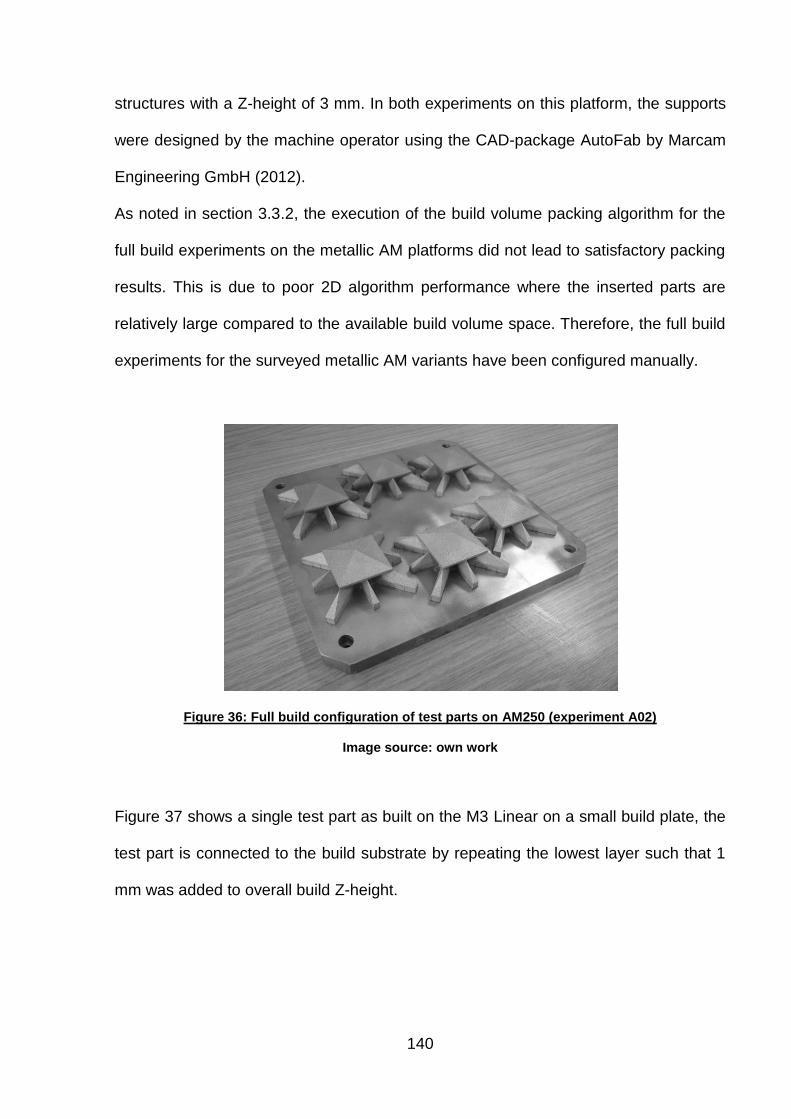
140

structures with a Z-height of 3 mm. In both experiments on this platform, the supports

were designed by the machine operator using the CAD-package AutoFab by Marcam

Engineering GmbH (2012).

As noted in section 3.3.2, the execution of the build volume packing algorithm for the

full build experiments on the metallic AM platforms did not lead to satisfactory packing

results. This is due to poor 2D algorithm performance where the inserted parts are

relatively large compared to the available build volume space. Therefore, the full build

experiments for the surveyed metallic AM variants have been configured manually.

Figure 36: Full build configuration of test parts on AM250 (experiment A02)

Image source: own work

Figure 37 shows a single test part as built on the M3 Linear on a small build plate, the

test part is connected to the build substrate by repeating the lowest layer such that 1

mm was added to overall build Z-height.

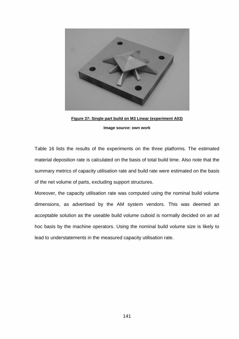
141

Figure 37: Single part build on M3 Linear (experiment A03)

Image source: own work

Table 16 lists the results of the experiments on the three platforms. The estimated

material deposition rate is calculated on the basis of total build time. Also note that the

summary metrics of capacity utilisation rate and build rate were estimated on the basis

of the net volume of parts, excluding support structures.

Moreover, the capacity utilisation rate was computed using the nominal build volume

dimensions, as advertised by the AM system vendors. This was deemed an

acceptable solution as the useable build volume cuboid is normally decided on an ad

hoc basis by the machine operators. Using the nominal build volume size is likely to

lead to understatements in the measured capacity utilisation rate.

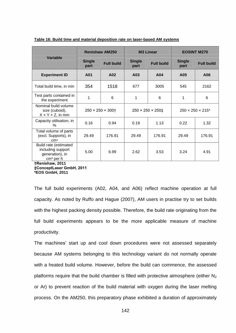
142

Table 16: Build time and material deposition rate on laser-based AM systems

Variable

Renishaw AM250 M3 Linear EOSINT M270

Single part

Full build Single part

Full build Single part

Full build

Experiment ID A01 A02 A03 A04 A05 A06

Total build time, in min 354 1518 677 3005 545 2162

Test parts contained in the experiment

1 6 1 6 1 6

Nominal build volume size (cuboid),

X × Y × Z, in mm 250 × 250 × 300† 250 × 250 × 250‡ 250 × 250 × 215*

Capacity utilisation, in %

0.16 0.94 0.19 1.13 0.22 1.32

Total volume of parts (excl. Supports), in

cmᶟ 29.49 176.91 29.49 176.91 29.49 176.91

Build rate (estimated including support

generation), in cm³ per h

5.00 6.99 2.62 3.53 3.24 4.91

†Renishaw, 2011 ‡ConceptLaser GmbH, 2011 *EOS GmbH, 2011

The full build experiments (A02, A04, and A06) reflect machine operation at full

capacity. As noted by Ruffo and Hague (2007), AM users in practise try to set builds

with the highest packing density possible. Therefore, the build rate originating from the

full build experiments appears to be the more applicable measure of machine

productivity.

The machines‟ start up and cool down procedures were not assessed separately

because AM systems belonging to this technology variant do not normally operate

with a heated build volume. However, before the build can commence, the assessed

platforms require that the build chamber is filled with protective atmosphere (either N2

or Ar) to prevent reaction of the build material with oxygen during the laser melting

process. On the AM250, this preparatory phase exhibited a duration of approximately

143

11 minutes. No corresponding measurement was obtained for the M3 Linear. On the

EOSINT M270, which is continuously flooded with N2, the start up procedure is very

rapid, measured at 63 s.

Overall maximum machine productivity is lowest on the M3 Linear (3.53 cm³ per h)

compared to the AM250 (6.99 cm³ per h) and the EOSINT M270 (4.91 cm³ per h). The

relatively small layer thickness on the M3 Linear, 30 μm, does not appear to be the

central determinant of the low build rate as it is the medium layer thickness in the

sample (50 μm on the AM250 and 20 μm on the EOSINT M270). A more plausible

reason is the time required by the M3 Linear to move its galvanometer assembly. This

system employs a galvanometer scanning optic which is moveable in the X/Y plane by

linear direct drives (ConceptLaser, 2007). This makes it necessary for the scanning

optic to process relatively small areas of each layer increment by increment.

After the scanning of a portion of the layer is complete, the linear drives move the

galvanometer to the next position where a further portion of the layer is scanned. This

is done to maintain the same level of accuracy over the entire powder bed

(ConceptLaser, 2007). It does however also decrease machine productivity as no

scanning is performed during galvanometer movement. In contrast to this, the

galvanometers in the AM250 and the EOSINT M270 are stationary, thus this extra

element of time consumption is absent.

5.1.1 Productivity building basket parts on the EOSINT M270

Following the experiments with the standard test part shown in Figure 20 (page 88) a

series of builds containing the basket parts was performed, as described above in

section 3.3.3.2. A full capacity build experiment was designed by executing the build

volume packing algorithm with excess demand dd for all parts. In the configuration

144

maintained throughout this thesis, the precedence vector p is ordered according to

part size. Thus, the first entry in p is the largest part (the bearing block) and the last

(fifth) entry is the smallest part in the basket (the venturi pipe).

The resulting full build configuration is shown in Figure 38. Of the available 2025 build

volume floor voxels, 92.6 % were occupied. A total of 85 parts were inserted; thus

utilizing 19.78 % of the net usable build volume cuboid (225 * 225 * 52 mm). To reflect

the 2.5D packing configuration, this statistic is reported with Z-height limited to the

space actually used by the basket parts.

In terms of the nominally available build volume space of 250 × 250 × 215 mm (with

full Z-height), a capacity utilisation rate of 3.7 % was achieved. It should be noted that

these results exclude the supports needed to anchor overhanging part geometries to

the substrate.

The employed build volume packing algorithm does not leave gaps between the voxel

approximations. However, gaps are maintained between the parts by positioning part

geometry within voxel approximations, as described in section 3.3.3.2. No element of

part geometry is allowed to be closer than 1 mm to the vertical boundaries of its voxel

approximation. Using this technique, a gap of at least 2 mm is therefore ensured

between each part in the build volume. This specification was chosen as the voxel

approximations have a low resolution (5 mm cubes). Thus, the gaps between the parts

are effectively determined in an earlier step of model construction during the

discretisation procedure. Using this methodology the gaps are pre-determined, which

may limit the applicability of this specification to DMLS. Other additive platforms may

require larger or smaller gaps.

It should also be mentioned that due to a flaw of the venturi part‟s design, combined

with ceramic blade of the EOSINT M270‟s powder deposition mechanism, a number of

145

these parts failed and were aborted in the final stage of the full build experiment. This

is deemed to have a negligible effect on the results of the model, however.

The bearing block and the turbine wheel were chosen for the single part builds (B02

and B03) because they exhibit very different surface/volume ratios. It was felt that it

would be interesting to test if the developed methodology is sensitive to this.

Figure 38: Full build configuration, basket parts (experiment B01)

Image source: own work

146

Table 17: Build time and material deposition rate on EOSINT M270

Variable

EOSINT M270

Full build of basket parts

Bearing block Turbine wheel Test part

(Figure 28)

Experiment ID B01 B02 B03 B04

Total build time, in min 6467 1555 520 82

Test parts contained in the experiment

85 1 1 1

Nominal build volume size (cuboid),

X × Y × Z, in mm 250 × 250 × 215†

Capacity utilisation, in %

3.70 0.72 0.15 0.03

Total volume of parts, in cm³

497.15 96.65 20.62 4.36

Build rate, in cm³ per h 4.61 3.73 2.38 3.19

†EOS GmbH, 2011

As Table 17 shows, the builds holding the basket parts (B01 to B03), the EOSINT

M270 exhibit build rates ranging from 2.38 to 4.61 cm³ per h. This indicates that the

properties of the test parts and the degree of capacity utilisation have a strong impact

on machine productivity.

Despite having the smallest layer thickness (20 µm) of all AM systems assessed, the

EOSINT M270 exhibits a higher build rate than the M3 Linear, which is probably due

to the fact that the EOSINT M270 has stationary galvanometer, as opposed to the

system on the M3 Linear which is moved in the X/Y plane, interrupting the exposure

process. Furthermore, the EOSINT M270 employs a stronger and more efficient 200

W fibre laser, compared to the 100 W Nd:YAG laser used on the M3 Linear.

It should be noted that the parts were manufactured on different machines and with

different materials. Therefore, they will not be identical. They exhibit differences in

147

mechanical properties, micro-structure, surface quality, accuracy, etc. This was not

assessed in this research

5.2 Electron beam melting

A single part experiment (A07) and a full build (A08), both based on the test geometry

shown in Figure 20 (page 88), were performed on the Arcam A1 EBM platform. In

these experiments, titanium (Ti-6Al-4V) test parts were constructed directly on the

steel substrate plate, thereby maximising heat transfer.

As the Arcam EBM process takes place with high powder bed temperatures of

approximately 700º C, a system warm up procedure is employed. Further, the build

activity takes place in vacuum, therefore an additional vacuum pulling procedure is

also required. The results of these two build experiment are listed in Table 18.

148

Table 18: Build time and material deposition rate for experiments on Arcam A1

Variable

A1

Single part Full build

Experiment ID A07 A08

Total build time, in min 206 300

Warm up time: machine start up, in min

23 10

Warm up time: preheating, in min 10 14

Build time, in min 155 260

Cool down, in min 17 17†

Test parts contained in the experiment

1 5

Nominal build volume size (cuboid), X × Y × Z, in mm

200 × 200 × 180‡

Capacity utilisation, in % 0.41 2.05

Total volume of parts, in cm³ 29.49 147.43

Build rate, in cm³ per h 8.59 29.49

† Cool down time estimated from single part data ‡ Arcam AB, 2011

The full build experiment (A08) contains 5 parts and was manually configured by the

machine operator as shown in Figure 39. The total build duration of the full build

experiment (300 min) is the shortest observed full build time in the sample.

Despite the build volume being the smallest of the assessed platforms, holding 5 test

parts, the resulting build rate of 29.49 cm³ per h of machine operation was the highest

in the sample. This is probably due to the relative large layer thickness setting of 70

μm in conjunction with extremely fast scanning speeds enabled by the electron beam

column (Chahine et al., 2008). The A1‟s electron beam has a nominal maximum

149

output rating of 3 kW (Arcam AB, 2011) which far exceeds the power of any available

laser based platform.

Figure 39: Full build configuration on Arcam A1 (experiment A08)

Image source: own work

5.3 Laser sintering

Next to assessing metallic AM systems, this thesis also investigates the productivity of

two polymeric AM technology variants, LS and FDM.

A single part experiment (A09) and a full build (A10), based on the power monitoring

geometry, were conducted on the EOSINT P390 (EOS GmbH, 2011). Two further

build experiments (C01 and C02) were conducted on two competing LS platforms, the

EOSINT P390 and the Sinterstation HiQ+HS (3D Systems, 2011).

To improve the economy of the full build experiment containing the standard test

parts, it was decided to restrict the experiment to a 50 mm portion of the available 600

mm of useful Z-height.

Figure 40 shows the 3D packing configuration resulting from the application of the

build volume packing algorithm in 3D mode. To achieve a relatively dense packing

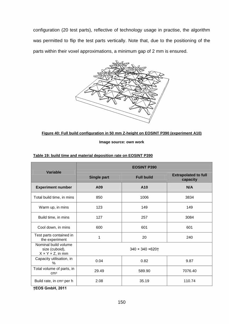
150

configuration (20 test parts), reflective of technology usage in practise, the algorithm

was permitted to flip the test parts vertically. Note that, due to the positioning of the

parts within their voxel approximations, a minimum gap of 2 mm is ensured.

Figure 40: Full build configuration in 50 mm Z-height on EOSINT P390 (experiment A10)

Image source: own work

Table 19: build time and material deposition rate on EOSINT P390

Variable

EOSINT P390

Single part Full build Extrapolated to full

capacity

Experiment number A09 A10 N/A

Total build time, in mins 850 1006 3834

Warm up, in mins 123 149 149

Build time, in mins 127 257 3084

Cool down, in mins 600 601 601

Test parts contained in the experiment

1 20 240

Nominal build volume size (cuboid),

X × Y × Z, in mm 340 × 340 ×620†

Capacity utilisation, in %

0.04 0.82 9.87

Total volume of parts, in cmᶟ

29.49 589.90 7076.40

Build rate, in cmᶟ per h 2.08 35.19 110.74

†EOS GmbH, 2011

151

The values reported in Table 19 in the column labelled „Extrapolated to full capacity‟

are estimates for a full build experiment using the full Z-height available (600 mm).

This is of importance as machine operators would in practise set builds with the

maximum possible degree of capacity utilisation (Ruffo and Hague, 2007). The

estimates are obtained by simply multiplying the core build time and the number of

parts contained by 12, which is the number of times the assessed 50 mm „slice‟ of Z-

height fits into the full 600 mm of usable build height. Corresponding estimates of full

capacity utilisation, volume of parts and build rate are also reported.

As Table 19 shows, the difference between the full build experiment and the single

part experiment in terms of build rate is dramatic. In the single part build the total build

rate is reported at 2.08 cm³ per h, which appears slightly lower than the deposition

rate exhibited on the metals platforms. However, during the full build experiment the

build rate was measured at 35.19 cm³ per h. If these results are adjusted to the whole

build volume, a build rate of 110.74 cm³ per h is estimated. This result is the highest

build rate observed across all build experiments. However, this also illustrates the

extreme importance of capacity utilisation for the process economics of LS, stemming

from the fixed process elements such as warm up and cool down.

5.3.1 Productivity building prosthetic sample parts on the EOSINT P390

Next to the experiments with dedicated testing geometries, two experiments involving

the construction of prosthetic sample parts were performed, as shown in Figure 41.

152

Figure 41: Full build configuration (experiments C01 and C02)

Total part volume: 1678.34 cm3, total part weight: 1562.5 g

Image source: own work

The build time results on the EOSINT P390 and the Sinterstation HiQ+HS are listed in

Table 20. It is shown that despite sharing the same operating principle, laser type,

layer thickness setting and build material (PA 12 type) the process duration is

relatively different for both platforms. The complete build experiment takes 1308

minutes on the Sinterstation HiQ+HS and 2301 minutes on the EOSINT P390.

These differences ultimately translate through to a significantly different build rate in

the experiments: while the Sinterstation HiQ+HS is able to deposit 76.99 cmᶟ of part

geometry per hour, the EOSINT P390 deposits only 43.76 cmᶟ in the same time

period. It should be noted that the warm up and cool down procedures are both more

time consuming on the EOSINT P390, further increasing the difference in the overall

build rate.

153

Table 20: Build time and material deposition rate on LS systems

Variable

EOSINT P390 Sinterstation HiQ+HS

Full build, prosthetic parts

Full build, prosthetic parts

Experiment ID C01 C02

Total build time, in min 2301 1308

Warm up, in min 171 107

Build time, in min 1530 1011

Cool down, in min 600 190

Test parts contained in the experiment

2 2

Nominal build volume size (cuboid), X × Y × Z, in mm

340 × 340 ×620† 381 × 330 × 457‡

Capacity utilisation, in % 2.34 2.92

Total volume of parts, in cm³ 1678.34 1678.34

Build rate, in cmᶟ per h 43.76 76.99

† EOS GmbH, 2011 ‡ 3D Systems, 2011

A comparison of the share of the different process phases (warm up, build time, cool

down) in is presented in Figure 42. While all three process phases take more time on

the EOSINT P390, the cool down procedure (600 min) appears to be especially

lengthy. During cool down the machine is not fully idle, temperature is reduced in a

controlled manner and the N2 build atmosphere is maintained.

154

Figure 42: Time consumption of process phases in LS

Image source: own work

This can be compared to the shares of process steps identified by Kellens et al.

(2010a) for the EOSINT P760, which is essentially a larger version of the EOSINT

P390. Figure 43 demonstrates that the relative share of the cool down procedure on

the EOSINT P390 may be quite extensive.

155

Figure 43: Time consumption of process phases in LS

Image source: own work, Kellens et al. (2010a)

The immediate insight yielded by these results is that the time consumption of the

warm up and cool down procedures in LS will have detrimental effect on the process

economics if the available build space is not utilised.

5.4 Fused deposition modelling

Two build experiments were performed on the Stratasys FDM400mc system. The first

held a single power monitoring geometry located in the centre of the build volume

(A11). The second experiment consisted of a full build of test parts (A12), organised

according to the build volume packing algorithm, as shown in Figure 44.

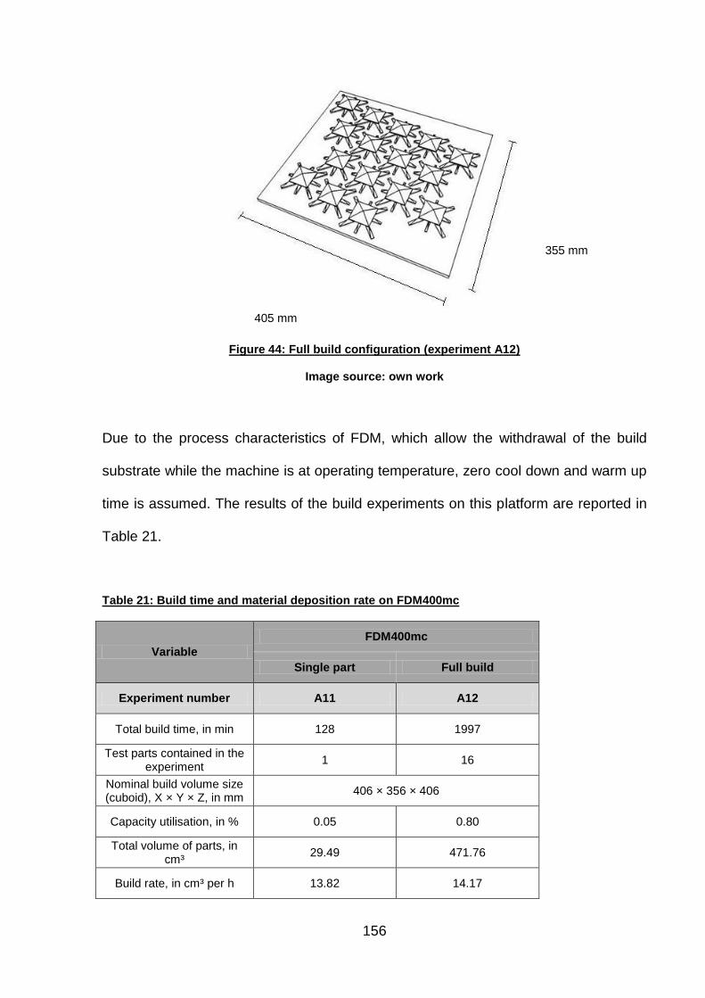
156

Figure 44: Full build configuration (experiment A12)

Image source: own work

Due to the process characteristics of FDM, which allow the withdrawal of the build

substrate while the machine is at operating temperature, zero cool down and warm up

time is assumed. The results of the build experiments on this platform are reported in

Table 21.

Table 21: Build time and material deposition rate on FDM400mc

Variable

FDM400mc

Single part Full build

Experiment number A11 A12

Total build time, in min 128 1997

Test parts contained in the experiment

1 16

Nominal build volume size (cuboid), X × Y × Z, in mm

406 × 356 × 406

Capacity utilisation, in % 0.05 0.80

Total volume of parts, in cm³

29.49 471.76

Build rate, in cm³ per h 13.82 14.17

405 mm

355 mm

157

These results show that, unlike the other assessed AM systems, machine productivity

on the FDM systems appears to be largely independent of capacity utilisation, with a

build rate of 13.82 cm³ per h in the single part build and 14.17 cm³ per h in the full

build. This result supports the hypothesis that fixed process elements (which are not

present in FDM), such as machine cool down, negatively affect AM process

economics if the available capacity is not fully utilised.

Moreover, the build volume packing result from the full build experiment yields some

insight to the performance of the packing algorithm, which is used in the 2D mode on

the FDM system. Figure 45 shows the file output schematic that was used to arrange

the build volume for the full build power monitoring experiment (A12). This image

shows the arrangement as an Excel spread sheet after the parts have been coloured

to aid identification.

Figure 45: Full build configuration on the FDM400mc (A12)

Image source: own work

158

Although the packing arrangement may appear inefficient at the build volume margins,

note the dense and regular ordering of the geometries in the build volume centre.

Although more research is needed to make a conclusive statement on the degree of

optimality exhibited by this configuration, it may well be that this arrangement in

slightly angled rows with interlocking „spider legs‟ maximises packing density.

It may therefore be speculated that, if build volume size increases to infinity and the

algorithm maintains this ordering for large problem instances, this packing approach

will lead to an efficient outcome – a promising result for an algorithm that is based on

the simple idea of agglomerating parts according to their centres of mass. This

observation also inspires confidence that the packing configurations with

heterogeneous parts (B01, B02, and B03) are also relatively efficient.

159

Chapter 6: Results on AM production input flows

After presenting the observed levels of productivity on the various additive machines

assessed in this research, the focus of chapter 6 moves to the results of the energy

consumption measurements obtained from power monitoring experiments and the

constructed combined build time, energy consumption and cost estimator.

As for chapter 5, the presented results address the requirement for reliable

productivity, energy consumption and cost data (encapsulated in research

objective II). Moreover, the constructed combined model of AM build time, energy

consumption and cost builds on these results. In this thesis, the combined model is

constructed and discussed for the EOSINT M270 DMLS system. The principles

relating to parallel manufacturing technology fundamental to this model should be

valid for all other AM technology variants discussed in this thesis, however.

6.1 Energy consumption results

This section presents power and energy consumption data for the various AM

technology variants. While data on the technology variants SLM, DMLS, EBM, and

FDM are presented, a special emphasis is placed on the results for the polymeric LS

platforms. This is done because the literature contains quite conflicting statements on

LS energy consumption: see, for example, Sreenivasan and Bourell (2009) versus

Kellens et al. (2010a). Furthermore, according to Ruffo et al. (2006b), polymeric LS

constitutes the most important additive technology variant for the manufacture of end-

use products.

160

6.1.1 Experimental results across systems

In the analysis of electric energy inputs, the two variables of interest are mean real

power consumption, reflecting the true power consumption of AC power systems, and

the total energy consumed. The results obtained from the full build experiments on the

various AM platforms should be reflective of machine operation at full capacity in real

world applications. Further, specific energy consumption per kg of part mass and per

cm³ of part volume are presented as summary metrics.

The build experiments performed on the ConceptLaser GmbH M3 Linear at the

Katholieke Universiteit Leuven in Belgium provided the opportunity to also test the

employed Yokogawa CW240 power monitoring setup for accuracy against another

power meter.

This was done by measuring real power consumption of the M3 Linear with two

meters installed simultaneously. The two meters used were the Additive

Manufacturing Research Group‟s Yokogawa CW240 (Figure 46a) and the Chauvin

Arnoux CA 8335+ (Figure 46b) belonging to the research group at Leuven. The power

meters were each attached to an independent set of voltage probes and current

clamps.

161

Figure 46: Digital power meters

Image source: own work

The real power consumption levels recorded by the meters were compared over an 8

h period during a build that was unrelated to this research. Figure 47 shows a

segment of the resulting data as overlaid graphs, indicating good congruence of the

measurements.

Figure 47: Digital power meters compared, CA 8335+ vs. CW240

Image source: own work

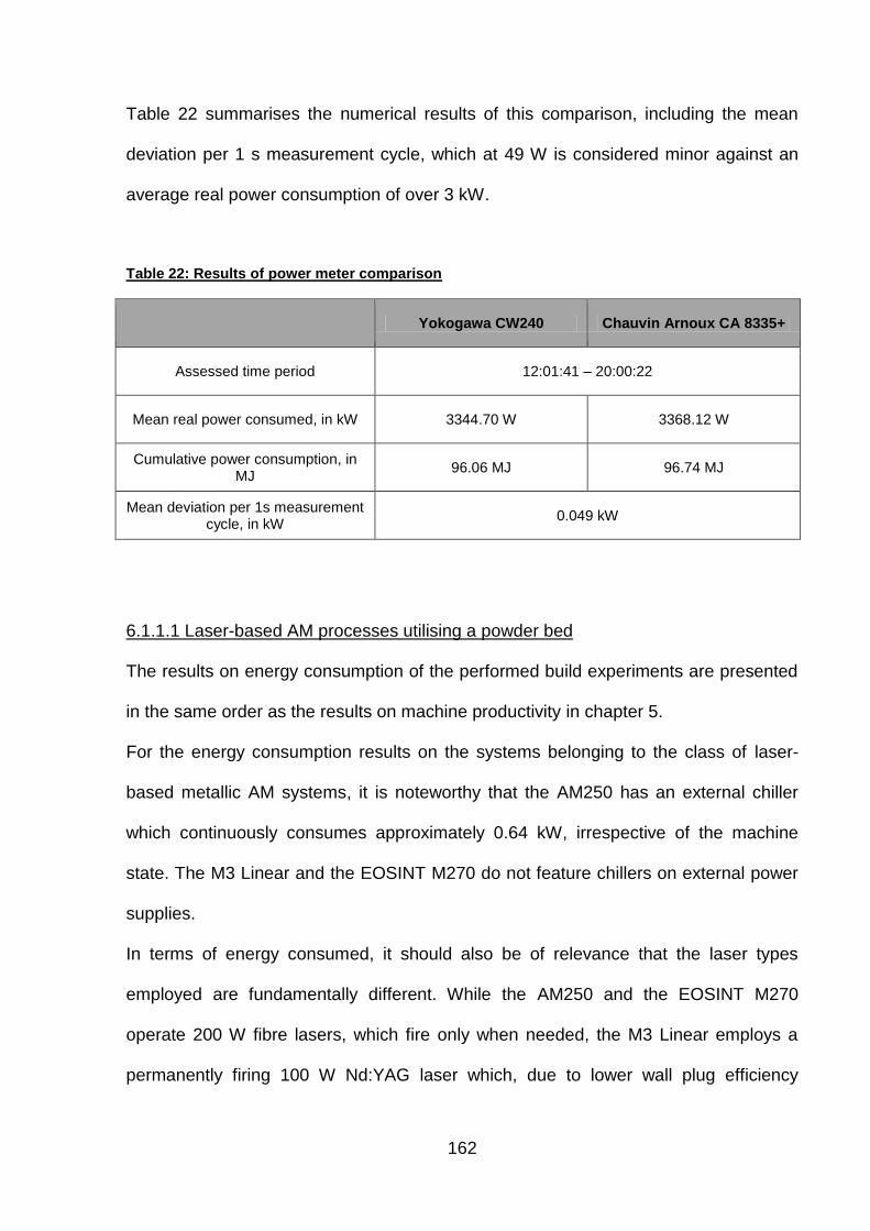
162

Table 22 summarises the numerical results of this comparison, including the mean

deviation per 1 s measurement cycle, which at 49 W is considered minor against an

average real power consumption of over 3 kW.

Table 22: Results of power meter comparison

Yokogawa CW240 Chauvin Arnoux CA 8335+

Assessed time period 12:01:41 – 20:00:22

Mean real power consumed, in kW 3344.70 W 3368.12 W

Cumulative power consumption, in MJ

96.06 MJ 96.74 MJ

Mean deviation per 1s measurement cycle, in kW

0.049 kW

6.1.1.1 Laser-based AM processes utilising a powder bed

The results on energy consumption of the performed build experiments are presented

in the same order as the results on machine productivity in chapter 5.

For the energy consumption results on the systems belonging to the class of laser-

based metallic AM systems, it is noteworthy that the AM250 has an external chiller

which continuously consumes approximately 0.64 kW, irrespective of the machine

state. The M3 Linear and the EOSINT M270 do not feature chillers on external power

supplies.

In terms of energy consumed, it should also be of relevance that the laser types

employed are fundamentally different. While the AM250 and the EOSINT M270

operate 200 W fibre lasers, which fire only when needed, the M3 Linear employs a

permanently firing 100 W Nd:YAG laser which, due to lower wall plug efficiency

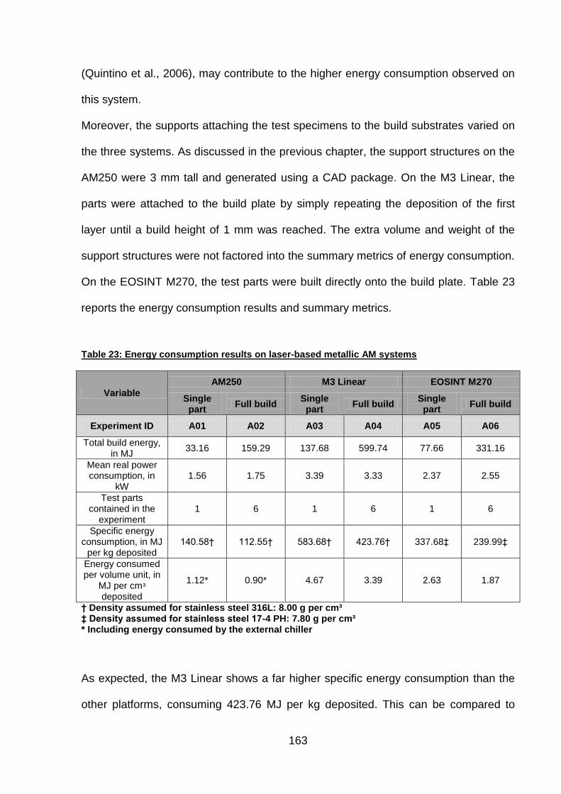
163

(Quintino et al., 2006), may contribute to the higher energy consumption observed on

this system.

Moreover, the supports attaching the test specimens to the build substrates varied on

the three systems. As discussed in the previous chapter, the support structures on the

AM250 were 3 mm tall and generated using a CAD package. On the M3 Linear, the

parts were attached to the build plate by simply repeating the deposition of the first

layer until a build height of 1 mm was reached. The extra volume and weight of the

support structures were not factored into the summary metrics of energy consumption.

On the EOSINT M270, the test parts were built directly onto the build plate. Table 23

reports the energy consumption results and summary metrics.

Table 23: Energy consumption results on laser-based metallic AM systems

Variable

AM250 M3 Linear EOSINT M270

Single part

Full build Single part

Full build Single part

Full build

Experiment ID A01 A02 A03 A04 A05 A06

Total build energy, in MJ

33.16 159.29 137.68 599.74 77.66 331.16

Mean real power consumption, in

kW 1.56 1.75 3.39 3.33 2.37 2.55

Test parts contained in the

experiment 1 6 1 6 1 6

Specific energy consumption, in MJ

per kg deposited 140.58† 112.55† 583.68† 423.76† 337.68‡ 239.99‡

Energy consumed per volume unit, in

MJ per cmᶟ deposited

1.12* 0.90* 4.67 3.39 2.63 1.87

† Density assumed for stainless steel 316L: 8.00 g per cm³ ‡ Density assumed for stainless steel 17-4 PH: 7.80 g per cm³ * Including energy consumed by the external chiller

As expected, the M3 Linear shows a far higher specific energy consumption than the

other platforms, consuming 423.76 MJ per kg deposited. This can be compared to

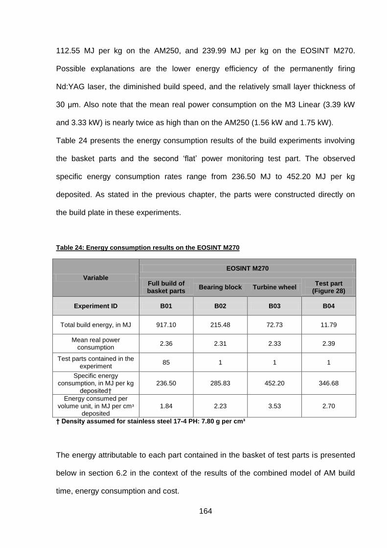
164

112.55 MJ per kg on the AM250, and 239.99 MJ per kg on the EOSINT M270.

Possible explanations are the lower energy efficiency of the permanently firing

Nd:YAG laser, the diminished build speed, and the relatively small layer thickness of

30 μm. Also note that the mean real power consumption on the M3 Linear (3.39 kW

and 3.33 kW) is nearly twice as high than on the AM250 (1.56 kW and 1.75 kW).

Table 24 presents the energy consumption results of the build experiments involving

the basket parts and the second „flat‟ power monitoring test part. The observed

specific energy consumption rates range from 236.50 MJ to 452.20 MJ per kg

deposited. As stated in the previous chapter, the parts were constructed directly on

the build plate in these experiments.

Table 24: Energy consumption results on the EOSINT M270

Variable

EOSINT M270

Full build of basket parts

Bearing block Turbine wheel Test part

(Figure 28)

Experiment ID B01 B02 B03 B04

Total build energy, in MJ 917.10 215.48 72.73 11.79

Mean real power consumption

2.36 2.31 2.33 2.39

Test parts contained in the experiment

85 1 1 1

Specific energy consumption, in MJ per kg

deposited† 236.50 285.83 452.20 346.68

Energy consumed per volume unit, in MJ per cmᶟ

deposited 1.84 2.23 3.53 2.70

† Density assumed for stainless steel 17-4 PH: 7.80 g per cm³

The energy attributable to each part contained in the basket of test parts is presented

below in section 6.2 in the context of the results of the combined model of AM build

time, energy consumption and cost.

165

On the laser-based metallic AM platforms assessed in this research, mean power

consumption results from 1.56 kW to 3.39 kW were observed. This corresponds

roughly to what has been observed by Mognol et al. (2006), 2.00 kW to 4.00 kW, and

Kellens et al. (2006b), reporting a mean real power consumption for LaserCusing from

2.25 kW to 3.45 kW.

The specific energy consumption observed in this research on the EOSINT M270

ranges from 236.50 MJ/kg to 452.20 MJ/kg. Using the data provided by Mognol et al.

(2006) the weight of their test part, as shown in Figure 17 (page 68), can be

approximated at 54.6 g (assuming a density of 7.80 g/cm³). Applying this to the

specific energy consumption reported by Mognol et al. (2006) of 32.00 kW to 56.00

kW per part, a specific energy consumption of 2109.89 MJ/kg to 3692.308 MJ/kg can

be approximated. Even though the test part used by Mognol et al. (2006) is smaller

(~7 cm³), than the parts assessed in single part builds in this research (27 cm³ to 97

cm³), this energy consumption result appears very high.

On the other hand, the specific energy consumption reported by Kellens et al. for the

M3 Linear LaserCusing system appears low: converted to MJ, a specific energy

consumption result of 96.82 MJ/kg can be approximated. The reason for this may lie in

the fact that the experiment this result is based on was short, lasting for only 4h,

indicating a high material deposition rate. No information on the geometry beyond the

mass of the sample parts (409 g) is given by Kellens et al. (2010a).

The energy consumption discussed in this research on the laser-based metallic

systems stand in stark contrast to the energy consumption results presented by

Morrow et al. (2007), who report power consumption levels of approximately 61 kW

and specific energy consumption rates in excess of 7700 MJ/kg. This may however be

due to the fact that the DMD process is conceptually very different from the assessed

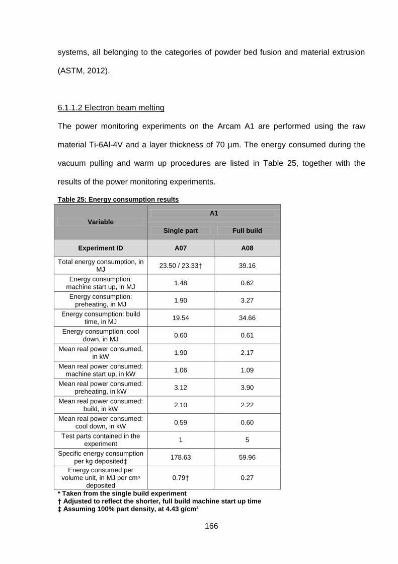
166

systems, all belonging to the categories of powder bed fusion and material extrusion

(ASTM, 2012).

6.1.1.2 Electron beam melting

The power monitoring experiments on the Arcam A1 are performed using the raw

material Ti-6Al-4V and a layer thickness of 70 µm. The energy consumed during the

vacuum pulling and warm up procedures are listed in Table 25, together with the

results of the power monitoring experiments.

Table 25: Energy consumption results

Variable

A1

Single part Full build

Experiment ID A07 A08

Total energy consumption, in MJ

23.50 / 23.33† 39.16

Energy consumption: machine start up, in MJ

1.48 0.62

Energy consumption: preheating, in MJ

1.90 3.27

Energy consumption: build time, in MJ

19.54 34.66

Energy consumption: cool down, in MJ

0.60 0.61

Mean real power consumed, in kW

1.90 2.17

Mean real power consumed: machine start up, in kW

1.06 1.09

Mean real power consumed: preheating, in kW

3.12 3.90

Mean real power consumed: build, in kW

2.10 2.22

Mean real power consumed: cool down, in kW

0.59 0.60

Test parts contained in the experiment

1 5

Specific energy consumption per kg deposited‡

178.63 59.96

Energy consumed per volume unit, in MJ per cmᶟ

deposited 0.79† 0.27

* Taken from the single build experiment † Adjusted to reflect the shorter, full build machine start up time ‡ Assuming 100% part density, at 4.43 g/cm³

167

Table 25 shows that the A1 system exhibits lower specific energy consumption than

the other metallic AM systems, with 178.63 MJ per kg in the single part experiment

and 59.69 MJ per kg in the full build. Due to the build process taking place in a

vacuum, a machine start up procedure involving vacuum pulling is necessary for each

build. It can be observed however, that the very high productivity of the EBM process

results in an energy efficient machine operation compared to the laser-based systems

presented in section 6.1.1.1. Further, the energy consumption of fixed process

elements (vacuum pulling, warm up, layer pre heating, and cool down), result in a

large discrepancy of the specific energy consumption result in the single part and full

build experiments. The relatively large layer thickness of 70 μm must also be seen as

a contributing factor to the energy efficiency of the system.

Besides the advantage in productivity, a factor contributing to the relative energy

efficiency of the A1 system is that it employs an electron beam instead of a laser.

According to Strutt (1980) energy transfer by electron beam is up to ten times more

efficient than energy transfer by laser.

6.1.1.3 Laser sintering

Four power monitoring experiments were performed on LS platforms for this research,

three of which were conducted on an EOSINT P390 and one on an Sinterstation

HiQ+HS. Table 26 and Table 27 show the energy consumption results for these

experiments, which all have a layer thickness setting of 100 µm. The build material in

the LS experiments is of the standard the PA 12 type (Nylon).

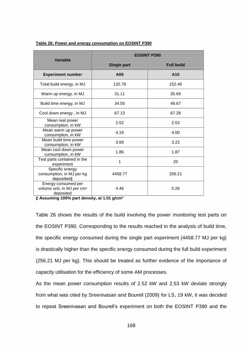
168

Table 26: Power and energy consumption on EOSINT P390

Variable EOSINT P390

Single part Full build

Experiment number A09 A10

Total build energy, in MJ 132.78 152.46

Warm up energy, in MJ 31.11 35.69

Build time energy, in MJ 34.55 49.67

Cool down energy , in MJ 67.13 67.28

Mean real power consumption, in kW

2.52 2.53

Mean warm up power consumption, in kW

4.19 4.00

Mean build time power consumption, in kW

3.69 3.22

Mean cool down power consumption, in kW

1.86 1.87

Test parts contained in the experiment

1 20

Specific energy consumption, in MJ per kg

deposited‡ 4458.77 256.21

Energy consumed per volume unit, in MJ per cmᶟ

deposited 4.46 0.26

‡ Assuming 100% part density, at 1.01 g/cm³

Table 26 shows the results of the build involving the power monitoring test parts on

the EOSINT P390. Corresponding to the results reached in the analysis of build time,

the specific energy consumed during the single part experiment (4458.77 MJ per kg)

is drastically higher than the specific energy consumed during the full build experiment

(256.21 MJ per kg). This should be treated as further evidence of the importance of

capacity utilisation for the efficiency of some AM processes.

As the mean power consumption results of 2.52 kW and 2.53 kW deviate strongly

from what was cited by Sreenivasan and Bourell (2009) for LS, 19 kW, it was decided

to repeat Sreenivasan and Bourell‟s experiment on both the EOSINT P390 and the

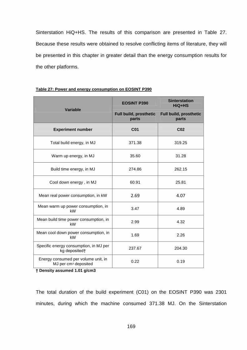
169

Sinterstation HiQ+HS. The results of this comparison are presented in Table 27.

Because these results were obtained to resolve conflicting items of literature, they will

be presented in this chapter in greater detail than the energy consumption results for

the other platforms.

Table 27: Power and energy consumption on EOSINT P390

Variable

EOSINT P390 Sinterstation

HiQ+HS

Full build, prosthetic parts

Full build, prosthetic parts

Experiment number C01 C02

Total build energy, in MJ 371.38 319.25

Warm up energy, in MJ 35.60 31.28

Build time energy, in MJ 274.86 262.15

Cool down energy , in MJ 60.91 25.81

Mean real power consumption, in kW 2.69 4.07

Mean warm up power consumption, in kW

3.47 4.89

Mean build time power consumption, in kW

2.99 4.32

Mean cool down power consumption, in kW

1.69 2.26

Specific energy consumption, in MJ per kg deposited†

237.67 204.30

Energy consumed per volume unit, in MJ per cmᶟ deposited

0.22 0.19

† Density assumed 1.01 g/cm3

The total duration of the build experiment (C01) on the EOSINT P390 was 2301

minutes, during which the machine consumed 371.38 MJ. On the Sinterstation

170

HiQ+HS (experiment C02), the production of the same parts took 1308 minutes, with a

total energy consumption of 319.25 MJ.

The purpose of the machines‟ warm up procedures is to prepare the systems for layer

scanning. In LS, parts need not be connected to a build plate, this normally makes the

deposition of a number of blank layers necessary. This procedure is normally at the

machine operator‟s discretion. It is included in the warm up procedure listed in Table

27.

Warm up on the Sinterstation HiQ+HS was carried out in 107 minutes; this includes

the sintering of an expendable heat shield at the bottom of the build volume. A total of

31.28 MJ were consumed (including the external optics chiller). The warm up

procedure on the EOSINT P390 was completed in 171 minutes using a total of

35.60 MJ.

Figure 48 and Figure 49 show the patterns of power consumption observed during

warm up on both platforms (experiments C01 and C02). The main trend observed on

both platforms is that once activated, machine power consumption decreases

gradually until build activity begins.

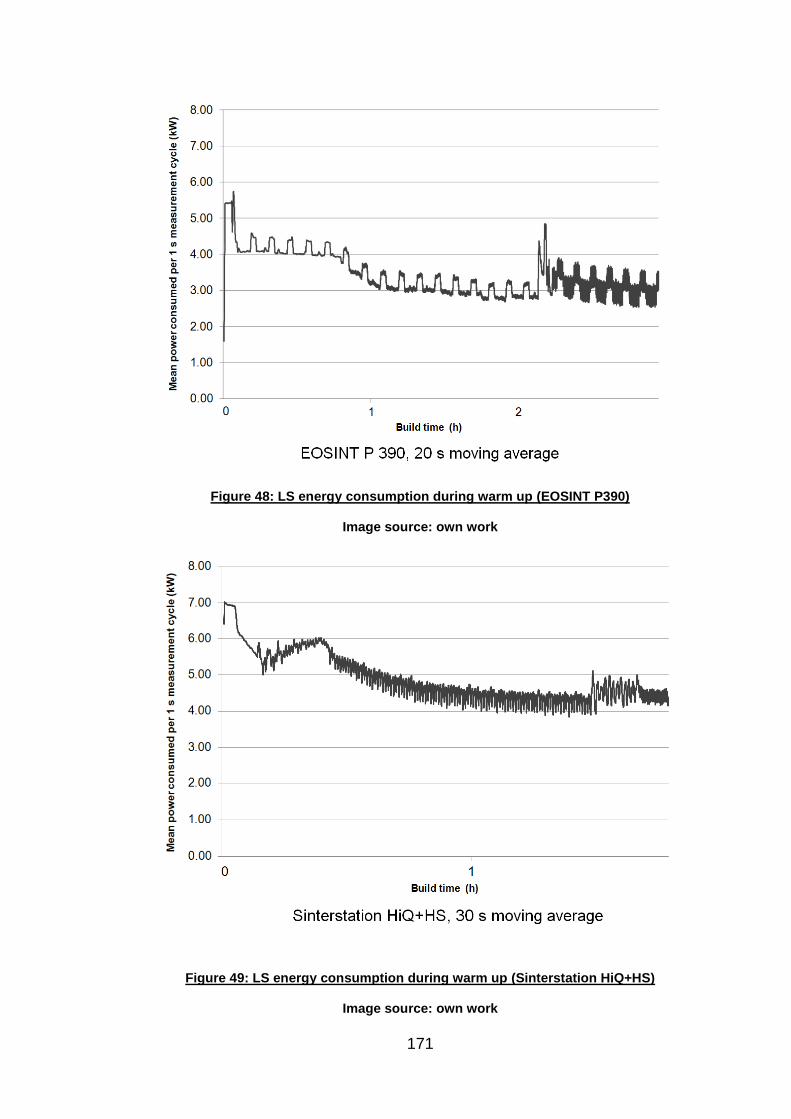
171

Figure 48: LS energy consumption during warm up (EOSINT P390)

Image source: own work

Figure 49: LS energy consumption during warm up (Sinterstation HiQ+HS)

Image source: own work

172

The duration of the core build time (during which the layer scanning and recoating

cycle takes place) varies significantly on the two platforms, from 1530 minutes on the

EOSINT P390 to 1011 minutes on the Sinterstation HiQ+HS, as shown in Figure 50

and Figure 51. The images also show a measure of baseline power consumption

occurring during the build phase. This measure is obtained by taking the minimum

energy consumption value of a moving 180 s interval of build time. Using this method,

a useful indicator of minimum energy consumption can be derived that is independent

of energy consumption fluctuations occurring during the sintering of each layer.

Figure 50: LS energy consumption during build time (EOSINT P390)

Image source: own work

173

Figure 51: LS energy consumption during build time (Sinterstation HiQ+HS)

Image source: own work

In terms of energy consumed during this phase, the Sinterstation‟s advantage in build

speed is almost completely offset by a higher mean power consumption (2.99 kWh vs.

4.32 kWh) resulting in a similar cumulative energy consumption (274.MJ vs. 262.15

MJ).

Following warm up and actual build activity, LS systems require a cool down

procedure; this is done to reduce part warpage resulting from uneven cooling (Held

and Pfligersdorffer, 2009). Duration and energy usage of the cool down procedure is

normally determined partly by the control system and partly by the operator, it may

thus vary considerably from build to build. Figure 52 and 53 present the real power

consumption during the cool down phases on the two LS platforms assessed

174

(experiments C01 and C02). The length of the cool down period varied strongly on

both platforms.

Figure 52: LS energy consumption during cool down (EOSINT P390)

Image source: own work

Figure 53: LS energy consumption during cool down (Sinterstation HiQ+HS) Image source: own work

175

Perhaps even more so than for warm up, finding the correct balance between

minimising cool down time and maintaining part integrity is determined by operator

skill. The power monitoring data (Table 27) show that the energy consumed during

this phase may vary considerably between different LS platforms.

Cool down on the EOSINT P390 was presented in roughly 600 minutes, during which

60.91 MJ were used. On the Sinterstation HiQ+HS, the cool down procedure lasted

approximately 190 minutes, during which a further 25.81 MJ were invested into the

parts. While the cool down procedure on the Sinterstation HiQ+HS exhibits a gradual

reduction of energy consumption, data from the EOSINT P390 show periodical spikes

(0.4 kW) of energy consumption and a constant mean level of power consumption.

This pattern may be caused by the system maintaining build volume temperature and

N2 process atmosphere.

A comparison of phase energy consumption shows that the energy expended for the

cool down procedure on the EOSINT P390 appears excessive, constituting 16.4% of

total energy consumption. It should be noted that on this platform the procedure is

determined by the control system and not by the machine operator. The minimum

permissible cool down duration for this build was selected.

The results reported here for the EOSINT P390 and the Sinterstation HiQ+HS may be

reconciled with those by Kellens et al. (2010b), who assess the energy consumption

on the EOSINT P760. This system is essentially a larger, dual laser version of the

EOSINT P390. This may explain the higher mean power consumption (8.28 kW vs.

2.99 kW) during the build time.

Moreover, the power consumed by the EOSINT P760‟s optics chiller, identified by

Kellens et al. as the greatest energy drain in the system, appears very high; it is

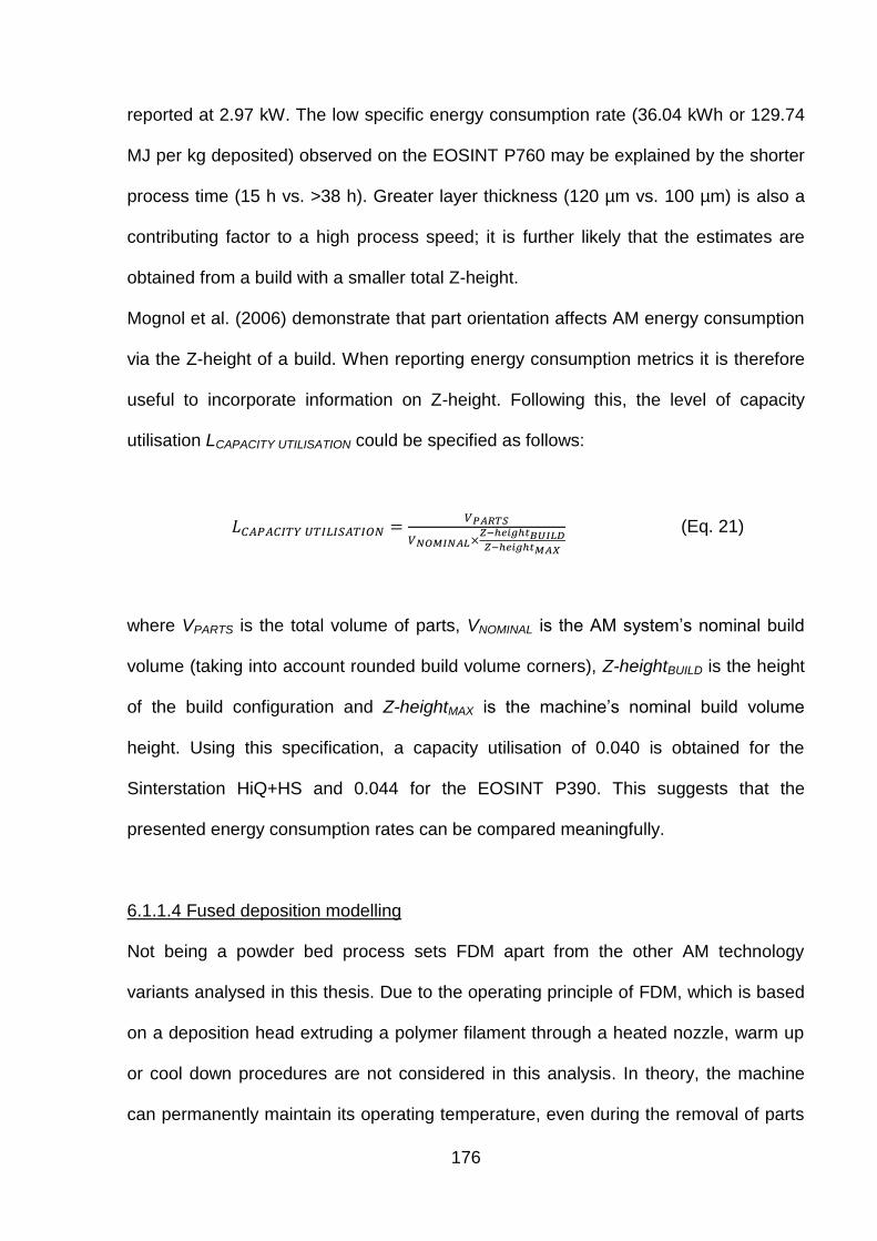
176

reported at 2.97 kW. The low specific energy consumption rate (36.04 kWh or 129.74

MJ per kg deposited) observed on the EOSINT P760 may be explained by the shorter

process time (15 h vs. >38 h). Greater layer thickness (120 µm vs. 100 µm) is also a

contributing factor to a high process speed; it is further likely that the estimates are

obtained from a build with a smaller total Z-height.

Mognol et al. (2006) demonstrate that part orientation affects AM energy consumption

via the Z-height of a build. When reporting energy consumption metrics it is therefore

useful to incorporate information on Z-height. Following this, the level of capacity

utilisation LCAPACITY UTILISATION could be specified as follows:

(Eq. 21)

where VPARTS is the total volume of parts, VNOMINAL is the AM system‟s nominal build

volume (taking into account rounded build volume corners), Z-heightBUILD is the height

of the build configuration and Z-heightMAX is the machine‟s nominal build volume

height. Using this specification, a capacity utilisation of 0.040 is obtained for the

Sinterstation HiQ+HS and 0.044 for the EOSINT P390. This suggests that the

presented energy consumption rates can be compared meaningfully.

6.1.1.4 Fused deposition modelling

Not being a powder bed process sets FDM apart from the other AM technology

variants analysed in this thesis. Due to the operating principle of FDM, which is based

on a deposition head extruding a polymer filament through a heated nozzle, warm up

or cool down procedures are not considered in this analysis. In theory, the machine

can permanently maintain its operating temperature, even during the removal of parts

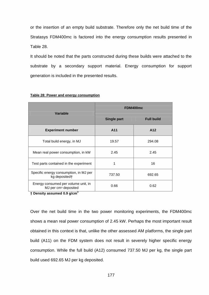
177

or the insertion of an empty build substrate. Therefore only the net build time of the

Stratasys FDM400mc is factored into the energy consumption results presented in

Table 28.

It should be noted that the parts constructed during these builds were attached to the

substrate by a secondary support material. Energy consumption for support

generation is included in the presented results.

Table 28: Power and energy consumption

Variable

FDM400mc

Single part Full build

Experiment number A11 A12

Total build energy, in MJ 19.57 294.08

Mean real power consumption, in kW 2.45 2.45

Test parts contained in the experiment 1 16

Specific energy consumption, in MJ per kg deposited†

737.50 692.65

Energy consumed per volume unit, in MJ per cmᶟ deposited

0.66 0.62

† Density assumed 0.9 g/cm3

Over the net build time in the two power monitoring experiments, the FDM400mc

shows a mean real power consumption of 2.45 kW. Perhaps the most important result

obtained in this context is that, unlike the other assessed AM platforms, the single part

build (A11) on the FDM system does not result in severely higher specific energy

consumption. While the full build (A12) consumed 737.50 MJ per kg, the single part

build used 692.65 MJ per kg deposited.

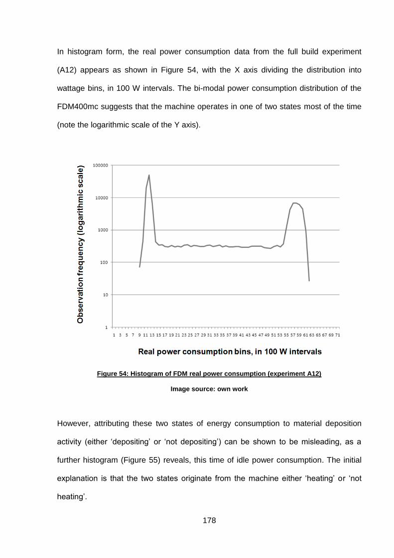
178

In histogram form, the real power consumption data from the full build experiment

(A12) appears as shown in Figure 54, with the X axis dividing the distribution into

wattage bins, in 100 W intervals. The bi-modal power consumption distribution of the

FDM400mc suggests that the machine operates in one of two states most of the time

(note the logarithmic scale of the Y axis).

Figure 54: Histogram of FDM real power consumption (experiment A12)

Image source: own work

However, attributing these two states of energy consumption to material deposition

activity (either „depositing‟ or „not depositing‟) can be shown to be misleading, as a

further histogram (Figure 55) reveals, this time of idle power consumption. The initial

explanation is that the two states originate from the machine either „heating‟ or „not

heating‟.

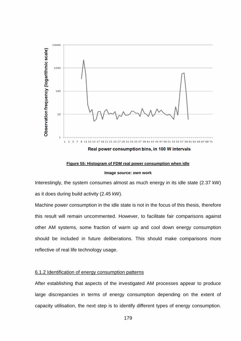
179

Figure 55: Histogram of FDM real power consumption when idle

Image source: own work

Interestingly, the system consumes almost as much energy in its idle state (2.37 kW)

as it does during build activity (2.45 kW).

Machine power consumption in the idle state is not in the focus of this thesis, therefore

this result will remain uncommented. However, to facilitate fair comparisons against

other AM systems, some fraction of warm up and cool down energy consumption

should be included in future deliberations. This should make comparisons more

reflective of real life technology usage.

6.1.2 Identification of energy consumption patterns

After establishing that aspects of the investigated AM processes appear to produce

large discrepancies in terms of energy consumption depending on the extent of

capacity utilisation, the next step is to identify different types of energy consumption.

180

The classification of energy consumption allows more structured statements on why

some AM variants exhibit certain patterns and others do not. Further, this classification

provides the starting point for the construction of a model of build time, energy

consumption and cost.

The data collected for the surveyed AM technology variants suggest that total energy

consumption can sensibly be split up into four categories:

Job dependent power consumption

Job dependent power consumption includes all fixed energy investments that

must be done for each AM build, irrespective of build parameters and

geometry. Examples for such power consumption are pre-heating energy

consumption during warm up and vacuum pump activity before a build.

Build time dependent power consumption

Build time dependent power consumption describes power consumption of

some AM subsystems depending purely on the length of the net build time.

Heater activity during net build time and control system power consumption

belong to this category.

Z-height dependent power consumption

Z-height dependent energy consumption can be attributed to the readying of

each new layer. Examples for such energy consumption are elevator and wiper

motor activity. Also, some processes activate build volume heaters cyclically for

each layer, for example in the laser sintering process (observed on the EOS

P390).

181

Geometry dependent power consumption

Geometry dependent power consumption, which constitutes a significant

proportion of energy consumption on most AM processes, is dependent on the

geometry of the parts contained in the build volume. Laser firing and

galvanometer activity in the LS and SLM processes fall in this category of

power consumption, as do energy expenditures for X/Y deposition head

movement in the FDM process. This is the constituent of energy consumption

that will depend directly on the volume of the produced parts and also their

shape.

Due to the comparative importance of the LS process in the production of end use

components (Ruffo et al., 2006b), the distinction of the different types of energy

consumption is discussed in the context of LS. The remainder of this section identifies

the four constituents of total energy consumption in the data collected on the EOSINT

P390 and the Sinterstation HiQ+HS.

As shown in Figure 50 and 51 (pages 172-173), the proportion of energy consumption

that depends on the net build time (during the actual build activity) can be singled out

relatively easily, by identifying the minimum energy consumption in a moving 180 s

interval.

During the build experiments performed on both systems (C01 and C02), total power

consumption and time dependent power consumption remain roughly constant

throughout the build activity. As expected for relatively large LS systems maintaining

elevated temperatures over prolonged periods, time dependent power consumption

contributes significantly to overall energy consumption.

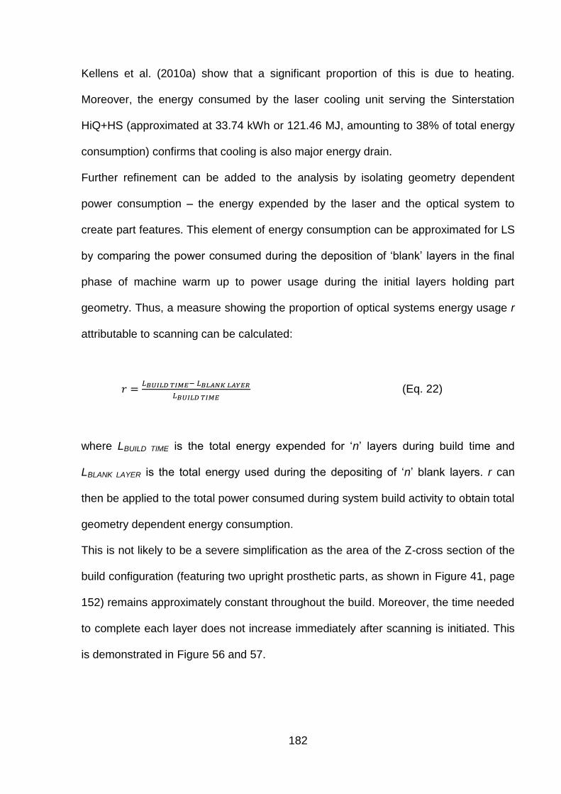
182

Kellens et al. (2010a) show that a significant proportion of this is due to heating.

Moreover, the energy consumed by the laser cooling unit serving the Sinterstation

HiQ+HS (approximated at 33.74 kWh or 121.46 MJ, amounting to 38% of total energy

consumption) confirms that cooling is also major energy drain.

Further refinement can be added to the analysis by isolating geometry dependent

power consumption – the energy expended by the laser and the optical system to

create part features. This element of energy consumption can be approximated for LS

by comparing the power consumed during the deposition of „blank‟ layers in the final

phase of machine warm up to power usage during the initial layers holding part

geometry. Thus, a measure showing the proportion of optical systems energy usage r

attributable to scanning can be calculated:

(Eq. 22)

where LBUILD TIME is the total energy expended for „n‟ layers during build time and

LBLANK LAYER is the total energy used during the depositing of „n‟ blank layers. r can

then be applied to the total power consumed during system build activity to obtain total

geometry dependent energy consumption.

This is not likely to be a severe simplification as the area of the Z-cross section of the

build configuration (featuring two upright prosthetic parts, as shown in Figure 41, page

152) remains approximately constant throughout the build. Moreover, the time needed

to complete each layer does not increase immediately after scanning is initiated. This

is demonstrated in Figure 56 and 57.

183

Figure 56: Geometry dependent power consumption in LS (EOSINT P390)

Image source: own work

Figure 57: Geometry dependent power consumption in LS (Sinterstation HiQ+HS)

Image source: own work

Of the total energy consumed, this approximation indicates that 4.48% (12.31 MJ) can

be attributed to geometry dependent power consumption on the EOSINT P390, based

184

on two blank layers and two scanned layers. On the Sinterstation HiQ+HS the

estimated geometry dependent power consumption is estimated at 5.43% (14.26 MJ),

this measure is obtained from three blank layers and three scanned layers. The result

that the geometry dependent energy approximations for both LS systems are similar

supports the validity of the analysis. This is to be expected as the prosthetic test parts

are identical and the laser systems in both machines have the same optical output

rating.

The job dependent element of power consumption can be identified in this analysis

simply by adding the energy expended for system warm up and cool down.

After subtracting job dependent, time dependent and geometry dependent energy

usage from total energy consumption, the remainder is viewed as Z-height dependent

energy consumption. Thus, a detailed picture emerges for both systems.

Figure 58: Identification of geometry dependent power consumption in LS

Image source: own work

It is an intuitive result that the extent of fixed job dependent energy consumption,

which should be equal across all builds on a platform, affects the degree to which

capacity utilisation matters. Because it is identical for each build, builds that hold a

185

greater quantity of parts or larger parts allow the amortization of such energy

consumption over a greater part quantity or part mass.

The second item of energy consumption that is amortised over the contents of the

build volume is the layer dependent energy consumption. This type of energy

consumption takes place every time a new layer is deposited, irrespective of what part

geometry is contained in that layer. Analogous to the case of job dependent energy

consumption, the layer dependent energy consumption is also amortised over part

volume and mass. However, an element of geometry dependency is present in this

type of energy consumption as the total number of layers in a build is determined by

the Z-height of the geometries contained in the build.

The two other elements of AM energy consumption, time dependent energy usage

and geometry dependent energy usage, are not amortised over the level of output.

The identification of the distinct types of AM system energy consumption serves as the

basis for the energy consumption element of the combined model of AM build time,

energy consumption and cost discussed in the following section.

6.1.3 A model of AM energy consumption

The classification of energy consumption elements flows into a model of energy

consumption as part of the combined model constructed in this thesis, applied to the

EOSINT M270 DMLS platform. The model specifications are obtained from a least

squares regressions of the time and energy consumption data recorded during the

deposition of each layer of the power monitoring test part in experiment B04. The

regressions use the area scanned per layer as the independent variable, resulting in

good functional fit with R² measures of 0.9869 (time) and 0.9935 (energy).

186

As clearly identifiable in the time and energy consumption data used in this regression

(shown in Figure 59), the test part is of layered design. This results in the four distinct

time and energy consumption levels for the vertical sections of the test part (as

illustrated in Figure 28, page 105).

Figure 59: Regressing cross-section area against time and energy consumption

Image source: own work

a)

b)

187

The obtained intercept parameters αTime (10.82 s) and αEnergy (0.008 MJ) are multiplied

by the number of layers in the build l in order to obtain layer dependent time and

energy consumption. The slope parameters expressing the time and energy

attributable to the scanning of 1 mm² during the build, βTime (0.0125 s) and βEnergy

(0.000013 MJ) are then used in conjunction with the layer thickness lt (0.02 mm) and a

measure of occupancy of each voxel to calculate total time and energy consumption

per voxel, TVoxel xyz and EVoxel xyz.

The rate of occupancy ROi in each voxel depends on the ratio of the volume of part i

occupying this voxel (VPi) and the volume of the voxel approximation for part i (VAi):

(Eq. 23)

Thus, for each (5 mm)³ voxel in the position xyz holding 250 (= 5 mm / lt) layers and

containing part i, the build time and energy consumption can be approximated:

(Eq. 24)

(Eq. 25)

Combining this with an estimated fixed time and energy consumption for machine start

up TJob (63 s) and EJob (0.125 MJ), the estimates of TBuild and EBuild are obtained as

follows. It should be noted that EBuild also contains the time dependent power

consumption, obtained by multiplying the base line energy consumption rate ĖTime

(0.0015 MJ per s) with TBuild.

∑∑ ∑

(Eq. 26)

188

(Ė ) ( ) ∑∑∑

(Eq. 27)

The specified time and energy consumption model can be validated by comparing the

calculated estimates to the real time and energy consumption during three build

experiments. Validation is performed for the full build at maximum machine capacity

(experiment B01, shown in Figure 38) and two builds of single components from the

basket of sample parts, the bearing block (B02) and the turbine wheel (B03). The

results of the validation experiments and the corresponding estimates of TBuild and

EBuild are presented in Table 29. Note that the validation does not include the energy

consumed by the ancillary wire erosion process.

It should also be mentioned that some of the venturi parts had an incorrect orientation

during the build, which, together with a design flaw, led to isolated build failure for the

affected parts in the final stages of the build. This is however deemed to have had a

negligible effect on the presented results.

Table 29: Confronting the estimates with experimental results

Experiment Time

consumed

Model estimate

TBuild Error

Energy usage

Model estimate

EBuild Error

Full Build experiment

(B01) 388031 s 354806 s -8.56% 917.10 MJ 879.93 MJ -4.05%

Single Bearing

block (B02) 93302 s 92338 s -1.03% 215.48 MJ 223.13 MJ 3.55%

Single Turbine

wheel (B03) 31224 s 28504 s -8.71% 72.73 MJ 66.80 MJ -8.15%

189

These results allow the calculation of a mean absolute error for build time (6.10%) and

for energy consumption (5.25%). The observed errors are likely to originate from the

use of an idealised test part shown in Figure 28 (page 105) in the experiments that

provided the data. Basing the estimation on real parts with a larger Z-height may have

increased the estimator‟s accuracy. This would have, however, come at the cost of

extremely large power monitoring files (to achieve the necessary time resolution, the

measurement cycle was set to 100 ms). Moreover, the build time estimator appears to

underpredict time consumption.

Nevertheless, the accuracy of the build time estimator compares favourably to the

accuracy of estimators of various kinds published in the literature. Table 30

summarises the performance of AM time estimators found in the literature against the

estimator proposed in this thesis.

190

Table 30: Time estimator performance in the literature

Publication Methodology Mean absolute

estimation error

Comments

This work Geometry-based

estimator 6.10%

Able to handle the multi-part, multi-product case

Ruffo et al., 2006a Parametric estimator 9.85%* Maximum error reported by

Ruffo at 13%

Campbell et al., 2008

Geometry-based estimator -4.54% A negative error indicates a

methodological problem

Materialise Magics (v.6.3) software performance

8.69%* Calculated from the data

provided by Campbell et al. (2008)

Munguia, 2009

Artificial neural network (non-parametric)

2.8% -

Ruffo et al., 2006a 14.98% -

Wilson, 2006 22.68% -

Di Angelo and Di Stefano, 2011

Artificial neural network (non-parametric)

12.00% -

* This value is not reported by the authors, it is calculated from data provided

The comparison of the results reported in the literature to the time estimator

developed in this thesis indicates that the developed estimation functionality performs

robustly. It should be stressed at this point that the estimators in the literature do not

tackle the problem of technical efficiency resulting from empty build volume capacity,

as described in section 2.3.3.

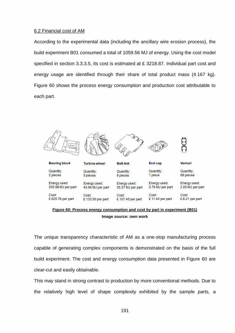
191

6.2 Financial cost of AM

According to the experimental data (including the ancillary wire erosion process), the

build experiment B01 consumed a total of 1059.56 MJ of energy. Using the cost model

specified in section 3.3.3.5, its cost is estimated at £ 3218.87. Individual part cost and

energy usage are identified through their share of total product mass (4.167 kg).

Figure 60 shows the process energy consumption and production cost attributable to

each part.

Figure 60: Process energy consumption and cost by part in experiment (B01)

Image source: own work

The unique transparency characteristic of AM as a one-stop manufacturing process

capable of generating complex components is demonstrated on the basis of the full

build experiment. The cost and energy consumption data presented in Figure 60 are

clear-cut and easily obtainable.

This may stand in strong contrast to production by more conventional methods. Due to

the relatively high level of shape complexity exhibited by the sample parts, a

192

conventional manufacturing route would likely require multiple operations to generate

the same “basket” parts. Depending on the supply chain configuration, these may be

carried out at different locations, resulting in further energy consumption and cost for

transportation and warehousing. Thus, the generation of matching estimates of the

overall energy usage and cost for the conventional route may well pose a significant

challenge.

193

Chapter 7: Discussion of results

In the previous chapters, the analysed topics are treated in a fixed order. The

discussion departs from this sequence. While maintaining the division line between

the benefits and costs of AM adoption (in monetary and energy terms), individual

discussion themes have crystallised out. The results reached in this thesis are

discussed in the context of these themes.

7.1 A discussion of the benefits to AM adoption

The review of the existing work on AM costing in section 2.3.3 criticises cost

estimators of the type proposed by Ruffo et al. (2006b). While this particular approach

is designed to estimate the manufacturing cost of AM products, its purpose is also to

serve as a decision making tool for potential AM technology adopters. The underlying

rationale is that the relationship between AM production cost and build quantity, as

postulated by Ruffo et al., can be used to determine break-even quantities at which

the average unit cost for different substitute technologies is equal. In the setup

discussed (Ruffo et al., 2006b), the cost of injection moulded parts is compared to the

cost of parts produced with LS.

This approach has been criticised in this thesis on the grounds that the downward

sloping cost function observed by Ruffo et al. for AM is obtained from configurations

with unused system capacity. It has been argued that this does not represent efficient

technology usage as AM users are in reality able to fill the available build space with

other, potentially unrelated, components. A practical strategy for the AM users to

mitigate the problem of excess capacity would be to replace the currently used AM

platform with a lower capacity system of the same technology variant.

194

However, there is a further limit to the usefulness of the technique used by Ruffo et al.

as a process decision tool. As Bernst (1975) argues, process choice should not be

made without exploring corresponding effects on material choice and product design.

This creates a dilemma: the choices of optimal process, design, and material are

interdependent, as illustrated in Figure 61. Thus, the different available alternatives in

manufacturing processes should not be evaluated without exploring effects on optimal

design and material specification.

Figure 61: Interdependence of part design, process and material choice

Image source: own work

When comparing different manufacturing processes, treating design as given ignores

AM‟s capability of realising complex geometry. For conventional manufacturing

processes, DFM is commonly used to tailor product design to the specifics of

manufacturing processes (Boothroyd et al., 1994; Bralla, 1998). Applied in the context

of conventional manufacturing alternatives, DFM dictates that design is adapted with

the limitations of the used process in mind.

With respect to AM‟s freedom of creating part geometry, as discussed by Hague et al.

(2004), a further qualification must be made: while AM may be considered less

195

restrictive, there are limitations that need to be considered. Different additive systems

will impose different manufacturability constraints (Xu et al., 1999). Among these are

minimum wall thickness, distortion, heat dissipation aspects, part orientation and

surface tolerances. While these factors will affect process selection decisions, they

may also affect part design. However, AM still places few constraints on design

(Hague et al., 2004) and there may be no requirement for the minimisation of design

complexity corresponding to the DFM methodology applied to more conventional

processes.

For these reasons, the problem of design/process/material interdependence inherent

to break-even analyses (e.g. based on cost functions) limits the usefulness of the

break-even approach, especially where heterogeneous technology is considered.

If a break even analysis is used despite these limitations, the used design must be

suitable for manufacturing on all considered platforms. However, this is likely to come

with disadvantages in terms of part functionality and performance. The resulting part

design may thus form the „smallest common denominator‟. From a product life cycle

view, it is highly unlikely that such products create the greatest net stream of benefits,

as discussed in the context of durable goods theory section 2.1.4.

Moreover, the use of a break-even approach to process adoption ignores that a very

important motivation for the uptake of new manufacturing processes is product

innovation: risking a statement of the obvious, Stoneman (2002) notes that the

technological advance embodied by a new product implies that it is somehow different

from the old version.

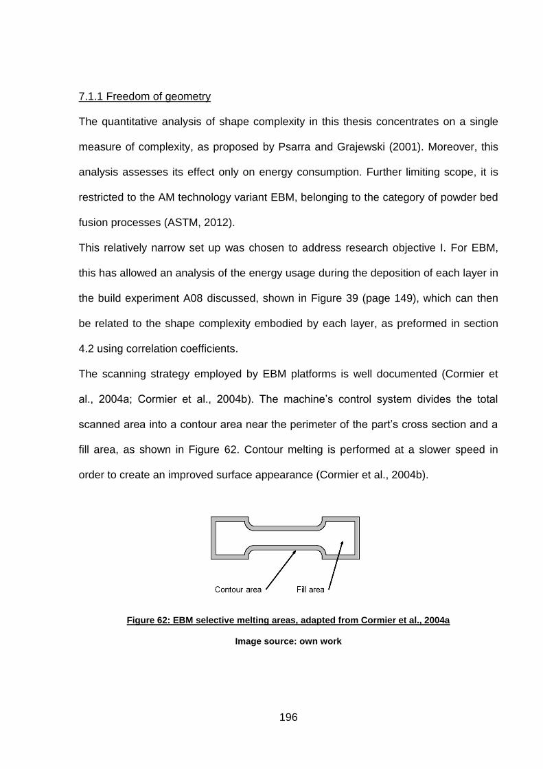
196

7.1.1 Freedom of geometry

The quantitative analysis of shape complexity in this thesis concentrates on a single

measure of complexity, as proposed by Psarra and Grajewski (2001). Moreover, this

analysis assesses its effect only on energy consumption. Further limiting scope, it is

restricted to the AM technology variant EBM, belonging to the category of powder bed

fusion processes (ASTM, 2012).

This relatively narrow set up was chosen to address research objective I. For EBM,

this has allowed an analysis of the energy usage during the deposition of each layer in

the build experiment A08 discussed, shown in Figure 39 (page 149), which can then

be related to the shape complexity embodied by each layer, as preformed in section

4.2 using correlation coefficients.

The scanning strategy employed by EBM platforms is well documented (Cormier et

al., 2004a; Cormier et al., 2004b). The machine‟s control system divides the total

scanned area into a contour area near the perimeter of the part‟s cross section and a

fill area, as shown in Figure 62. Contour melting is performed at a slower speed in

order to create an improved surface appearance (Cormier et al., 2004b).

Figure 62: EBM selective melting areas, adapted from Cormier et al., 2004a

Image source: own work

197

Taking into account the electron beam‟s potentially extreme scanning speed of up to

1,000 m per second (Chahine et al., 2008), there may be no direct relationship

between the intricacy of the shape or its dispersion in the X/Y plane and the energy

expended to melt the layer. Total melting energy consumption per layer „i‟ can be

assumed to be the result of the sum of energy consumed for contour melting and the

energy consumed to fill in the contours:

FILLFILLCONTOURCONTOURi AIAIenergymeltingLayer (Eq. 28)

where ICONTOUR is the energy intensity used to melt contour area ACONTOUR and IFILL is

the energy intensity used to fill in the shape, area AFILL. However, it has been shown

that melting energy consumption for the EBM process correlates heavily with total

layer area, which makes a distinction between contour and fill area unnecessary.

Using the Pearson correlation coefficients, it has been argued that in EBM melting

energy is independent of the specifics of shape and geometry (and instead depends

exclusively on melting area). This is supported by the results presented above in

section 4.2:

6568.0, ENERGYLAYERPERIMETER (Eq. 29)

8263.0, ENERGYLAYERAREA (Eq. 30)

3544.0, ENERGYLAYERMCV (Eq. 31)

Thus, the creation of elements of extra shape complexity may not require extra

process energy consumption if not accompanied by increased scanning area. This

potentially allows the provision of additional functionality at zero marginal energy

consumption.

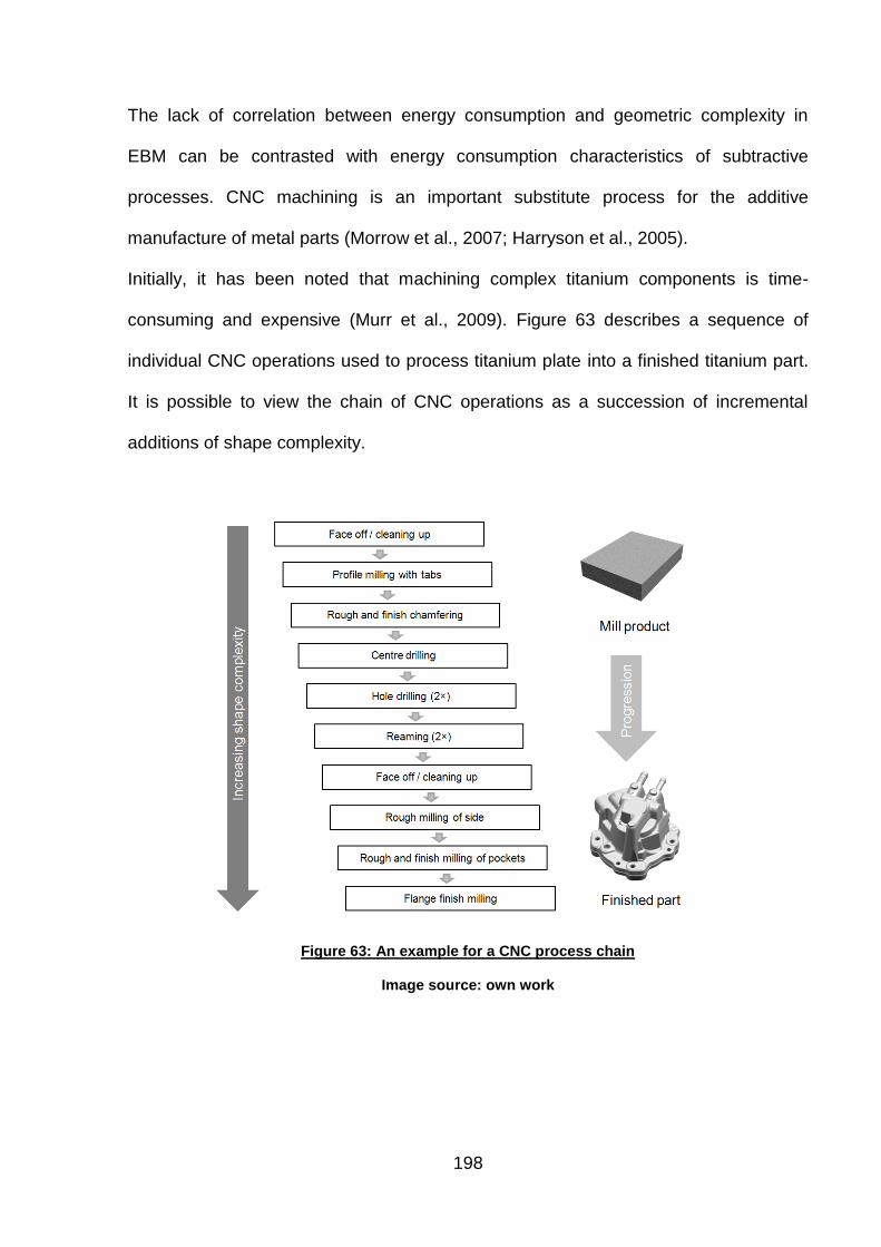
198

The lack of correlation between energy consumption and geometric complexity in

EBM can be contrasted with energy consumption characteristics of subtractive

processes. CNC machining is an important substitute process for the additive

manufacture of metal parts (Morrow et al., 2007; Harryson et al., 2005).

Initially, it has been noted that machining complex titanium components is time-

consuming and expensive (Murr et al., 2009). Figure 63 describes a sequence of

individual CNC operations used to process titanium plate into a finished titanium part.

It is possible to view the chain of CNC operations as a succession of incremental

additions of shape complexity.

Figure 63: An example for a CNC process chain

Image source: own work

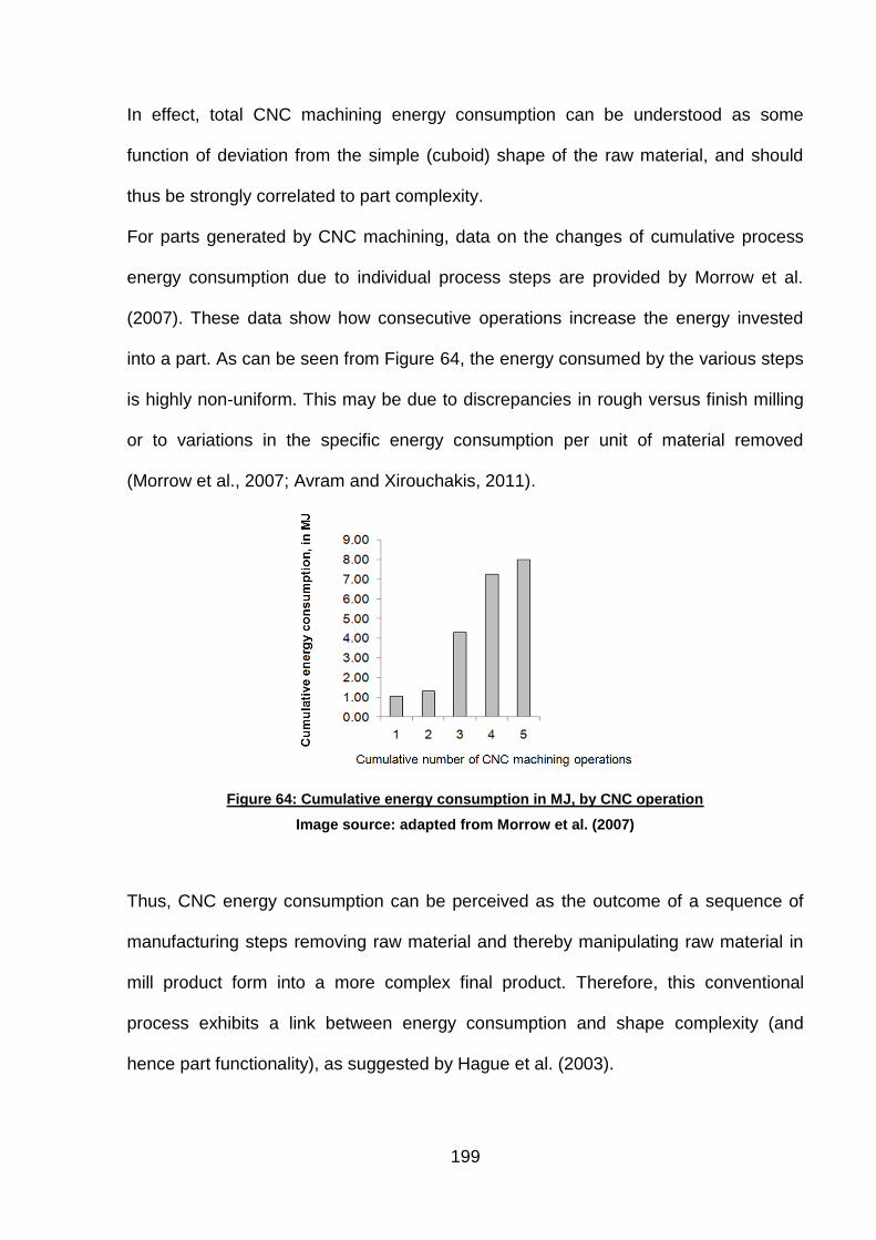
199

In effect, total CNC machining energy consumption can be understood as some

function of deviation from the simple (cuboid) shape of the raw material, and should

thus be strongly correlated to part complexity.

For parts generated by CNC machining, data on the changes of cumulative process

energy consumption due to individual process steps are provided by Morrow et al.

(2007). These data show how consecutive operations increase the energy invested

into a part. As can be seen from Figure 64, the energy consumed by the various steps

is highly non-uniform. This may be due to discrepancies in rough versus finish milling

or to variations in the specific energy consumption per unit of material removed

(Morrow et al., 2007; Avram and Xirouchakis, 2011).

Figure 64: Cumulative energy consumption in MJ, by CNC operation

Image source: adapted from Morrow et al. (2007)

Thus, CNC energy consumption can be perceived as the outcome of a sequence of

manufacturing steps removing raw material and thereby manipulating raw material in

mill product form into a more complex final product. Therefore, this conventional

process exhibits a link between energy consumption and shape complexity (and

hence part functionality), as suggested by Hague et al. (2003).

200

It must be remarked that there is a discrepancy between EBM and conventional

manufacturing processes in terms of surface quality. Ponader et al. (2007)

demonstrate that the surface smoothness of conventionally manufactured parts far

surpasses the smoothness of EBM products. For polished surfaces (SiC, 2400 grit) an

Ra value of 0.077 µm is cited. For corresponding EBM test parts, manufactured in

different orientations, Ra values ranging from 24.9 µm to 96.7 µm are reported

(Ponader et al., 2007). Therefore, EBM parts will normally be subject to light finish

machining (Cormier et al., 2004a) or shot blasting (Mazzioli et al., 2009) requiring

further energy inputs, which are not included in this analysis.

7.1.2 Complementarity, network effects and hierarchy of innovations

Considering the different manufacturing philosophies discussed in the literature review

(Tuck, 2007; Milgrom and Roberts, 1995) it is an interesting question to ask whether

the performance dimensions against which a manufacturing technology is evaluated

should differ according to the manufacturing philosophy.

For example, should a technology that is employed in „lean‟ mass production be

judged against the same performance dimensions as AM process technology?

As noted by Patel and Pavitt (1995) there is the additional issue of how to weight

multiple dimensions of technical performance.

As Milgrom and Roberts (1995) argue, success in modern manufacturing is an issue

of whether a firm can capitalise on the complementarities that lie in its processes and

technologies. In other words, success appears to be determined by how well the

involved technologies and organisational forms „fit‟. Therefore, in comparative

analyses of different manufacturing process technologies, the used weighting and

dimensions should reflect organisational strategy and goals.

201

In section 2.1.5.1 it is argued that the benefits of an introduction of AM technology will

be determined by the use of 3D CAD technology in the organisation. Where the

benefits arising from combined technology adoption exceed the sum of the benefits

that can be obtained from adopting the technologies individually, Stoneman (2002)

describes such technologies as complementary.

However, identifying AM and 3D CAD as complements may not characterise the

relationship between the technologies sufficiently well. Hague (2004) has noted that

the use of 3D CAD is required for all modern manufacturing technologies. This

suggests that that the relationship between 3D CAD and AM is in fact one of

hierarchy.

A framework for the determination of the hierarchies existing among technologies is

presented by Coccia (2004). This leads to the suggestion that 3D CAD technology

may constitute a higher-order process innovation in relation to AM technology.

While it is clear that information technology forms a technological prerequisite to AM, it

is interesting to explore to what extent AM technology can be interpreted as a novel

form of „output device‟ for computers, perhaps similar to printer hardware. Following

the intuition of viewing AM as a further form of computer hardware instead of an

innovation in its own right, the public and media have adopted the term „three

dimensional printing‟ as a de facto name to collectively describe all AM technology

(Wohlers, 2011b). Under this moniker, AM has received considerable media attention

(see, for example, The Economist, 2010). Recognising AM‟s dependence on computer

hardware and software, the classification as a lesser order innovation following the

introduction of 3D CAD appears appropriate.

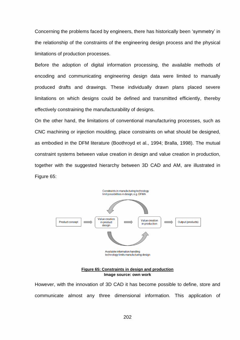
202

Concerning the problems faced by engineers, there has historically been „symmetry‟ in

the relationship of the constraints of the engineering design process and the physical

limitations of production processes.

Before the adoption of digital information processing, the available methods of

encoding and communicating engineering design data were limited to manually

produced drafts and drawings. These individually drawn plans placed severe

limitations on which designs could be defined and transmitted efficiently, thereby

effectively constraining the manufacturability of designs.

On the other hand, the limitations of conventional manufacturing processes, such as

CNC machining or injection moulding, place constraints on what should be designed,

as embodied in the DFM literature (Boothroyd et al., 1994; Bralla, 1998). The mutual

constraint systems between value creation in design and value creation in production,

together with the suggested hierarchy between 3D CAD and AM, are illustrated in

Figure 65:

Figure 65: Constraints in design and production

Image source: own work

However, with the innovation of 3D CAD it has become possible to define, store and

communicate almost any three dimensional information. This application of

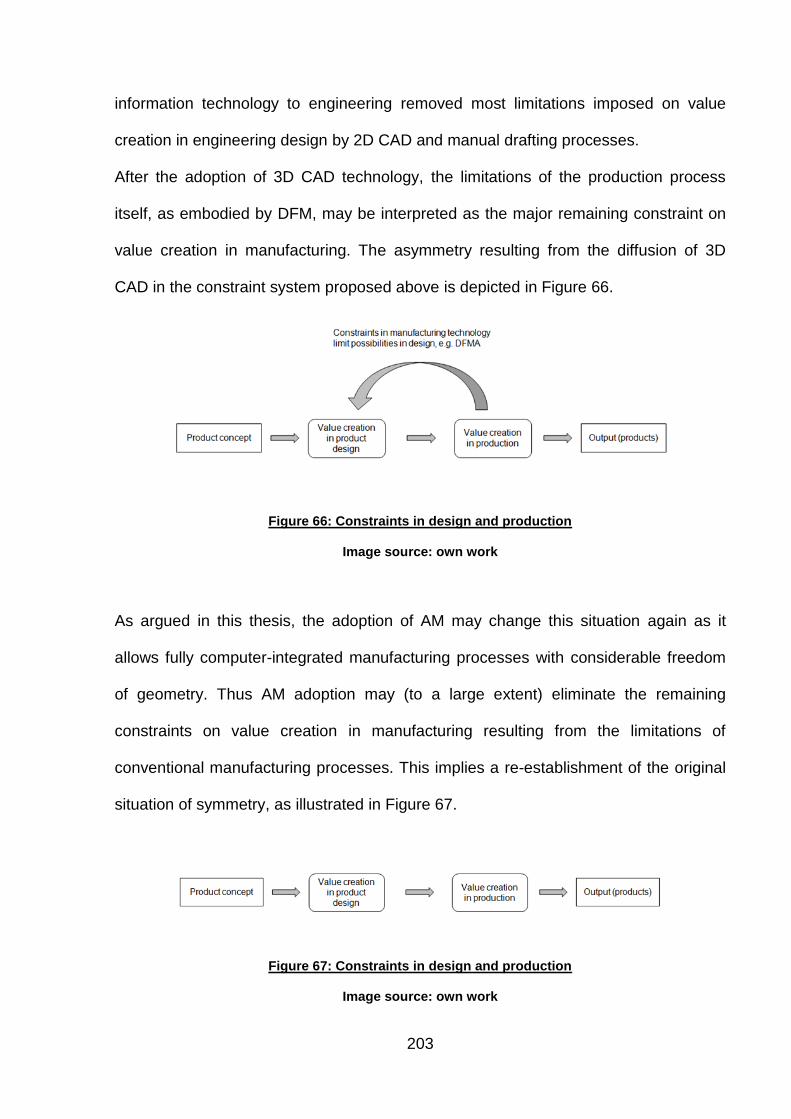
203

information technology to engineering removed most limitations imposed on value

creation in engineering design by 2D CAD and manual drafting processes.

After the adoption of 3D CAD technology, the limitations of the production process

itself, as embodied by DFM, may be interpreted as the major remaining constraint on

value creation in manufacturing. The asymmetry resulting from the diffusion of 3D

CAD in the constraint system proposed above is depicted in Figure 66.

Figure 66: Constraints in design and production

Image source: own work

As argued in this thesis, the adoption of AM may change this situation again as it

allows fully computer-integrated manufacturing processes with considerable freedom

of geometry. Thus AM adoption may (to a large extent) eliminate the remaining

constraints on value creation in manufacturing resulting from the limitations of

conventional manufacturing processes. This implies a re-establishment of the original

situation of symmetry, as illustrated in Figure 67.

Figure 67: Constraints in design and production

Image source: own work

204

The described absence of constraints on value creation in the design phase as well as

the production phase point to the conclusion that AM adoption promises significant

productivity increases in manufacturing. Therefore, this section argues that that the

minimally restrictive nature of 3D CAD in the engineering design process is

complemented through AM adoption by introducing a matching, geometrically

minimally restrictive, production process.

In consequence, it appears justified to interpret both 3D CAD and AM as „spill overs‟

from IT, which belongs to the class of general purpose technologies (GPTs). As

discussed in section 2.1.5.4, GPTs are characterised by such inter-sectoral spill over

effects (Stoneman, 2002), their role in economic growth (Bresnahan and Trajtenberg,

1995) and their impact on domestic life and business activity (Jovanovic and

Rousseau, 2005).

The classification of AM as a GPT, or alternatively as an extension of IT, may provide

some insight into future diffusion patterns. The diffusion of GPTs may begin slower

than for other technologies with more restricted applications (Jovanovic and

Rousseau, 2005). This may be due to the time needed for the technology and the

input markets to develop.

However, it may well be that there are also considerable network effects between AM

adopters, which may accelerate diffusion speed once a critical number of adopters is

reached. As the 3D data used in AM equipment in the standard *.stl format is

interchangeable, AM adopters may find it profitable to pool demand to realise

maximum capacity utilisation. This kind of network effect is indicative of GPTs

according to Stoneman (2002). The business models of AM service providers such as

Shapeways (Shapeways, 2011) of Fabberhouse (Fabberhouse, 2011) may be

evidential of this.

205

7.2 A discussion of results on machine productivity, energy and cost

The investigation of build time, energy consumption and cost performed for this

research has led to the identification of three themes for discussion. The first theme

considers the empirical evidence collected with respect to the degree to which the

observed degree of capacity utilisation matters. Here, the focus lies on energy

consumption, as discussed in section 7.2.1. However, the mechanisms governing the

relationship between capacity utilisation and energy consumption may be the same

that govern the relationship between capacity utilisation and the financial cost of AM.

The combined build time, energy consumption and cost estimator developed for the

AM technology variant DMLS is discussed in section 7.2.2. The estimator is applied to

different demand profiles faced by the DMLS users. It is argued that the adopter‟s

ability to fill the build volume is the prime determinant of AM cost and energy

efficiency.

The final theme of discussion reflects that the results reached in this thesis can be put

into the context of a life-cycle centric assessment of the economics of AM. It is argued

in section 7.2.3 that production cost focussed approaches to the manufacture of

complex and advanced durable goods may hinder the exploitation of the capabilities

offered by geometrically unrestrictive manufacturing technologies such as AM.

206

7.2.1 The dual problem with the break even cost model

As discussed in the context of the benefits of AM methodologies in section 7.1, break

even costing models postulating relationships between the production quantity and the

marginal cost of output may not be able to capture the capabilities of geometrically

less restrictive manufacturing processes to create complex products.

This thesis has attempted to make the case that methodologies hinging on leaving

machine capacity unused are not indicative of AM technology usage in practise, let

alone efficient commercial AM operations where demand may be pooled. This

problem is likely to apply to all manufacturing approaches allowing the

contemporaneous generation of products, labelled “parallel” manufacturing technology

by Ruffo et al. (2006b).

The effect of capacity utilisation on the process efficiency of major AM technology

variants has been assessed in this thesis with respect to productivity and energy

consumption. The process energy consumption results obtained from the performed

power monitoring experiments show that the various assessed AM technology

variants exhibit different energy consumption levels when the degree of capacity

utilisation changes. However, the extent of this difference varies strongly across the

assessed systems.

Figure 68 shows that for every AM platform, the full build experiment results in

different specific energy consumption levels in the full build and single part

experiments. It is noteworthy that on all platforms the switch from single part to full

build operation has resulted in a reduction of specific energy consumption.

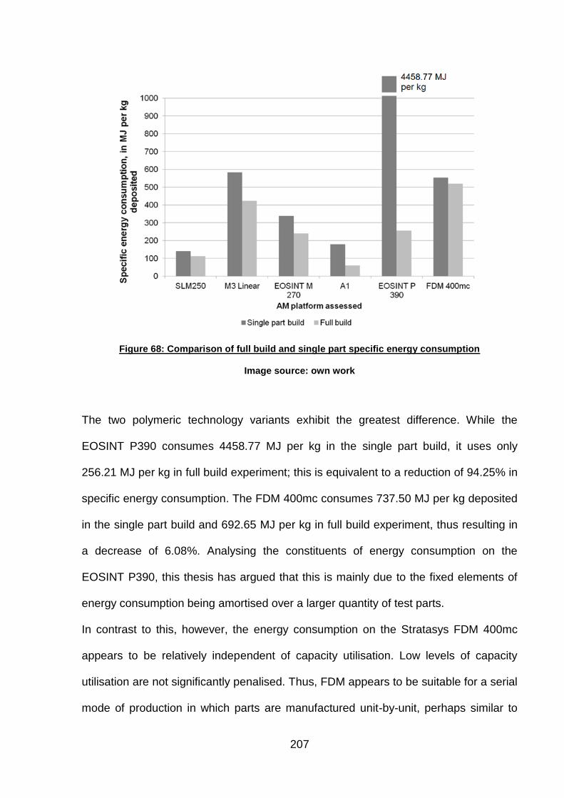
207

Figure 68: Comparison of full build and single part specific energy consumption

Image source: own work

The two polymeric technology variants exhibit the greatest difference. While the

EOSINT P390 consumes 4458.77 MJ per kg in the single part build, it uses only

256.21 MJ per kg in full build experiment; this is equivalent to a reduction of 94.25% in

specific energy consumption. The FDM 400mc consumes 737.50 MJ per kg deposited

in the single part build and 692.65 MJ per kg in full build experiment, thus resulting in

a decrease of 6.08%. Analysing the constituents of energy consumption on the

EOSINT P390, this thesis has argued that this is mainly due to the fixed elements of

energy consumption being amortised over a larger quantity of test parts.

In contrast to this, however, the energy consumption on the Stratasys FDM 400mc

appears to be relatively independent of capacity utilisation. Low levels of capacity

utilisation are not significantly penalised. Thus, FDM appears to be suitable for a serial

mode of production in which parts are manufactured unit-by-unit, perhaps similar to

208

the strictly serial mode of injection moulding machines. Compared to the full capacity

energy consumption result on the EOSINT P390 however, the FDM400mc system

exhibits significantly higher specific energy consumption during full capacity operation.

The reason for this appears to be the absence of fixed increments of energy

consumption that must be amortised over a build. These can be job-specific (for

example, warm up procedures) or layer-specific (for example fresh powder

deposition). Moreover, the small energy efficiency gains realised from parallel

manufacturing in FDM are perhaps even outweighed in the real business environment

by the potential savings derived from retrieving parts as early as possible from the

build volume.

It should be remarked at this point that support generation was determined by the

machine operators during the build experiments. For a more consistent assessment of

AM energy consumption (and of process economics), it would be beneficial to perform

support generation in a more uniform way. In the process of this research, the guiding

principle was to leave these decisions to the machine operators. This may have

slightly skewed the results.

Further insight into the impact of capacity utilisation on the process of economics of

the various assessed AM processes can be won through the analysis of the effect on

the build rate, measured in cm³ of material deposited per h.

As argued throughout this thesis, build time is an important determinant of both

production cost and energy consumption. The scatter diagram in Figure 69 plots the

build rate in all 18 build experiments against the nominal capacity utilisation rates

(presented in chapters 5 and 6).

209

Figure 69: Nominal capacity utilisation rate vs. Build rate

Image source: own work

Figure 69 shows that on all platforms (except the Sinterstation HiQ+HS, on which only

one experiment was performed), the material deposition rate is positively related to

capacity utilisation.

Capacity utilisation had a particularly strong effect on system productivity on the

EOSINT P390 and the A1 which are systems that require extensive warm up or cool

down procedures and feature a relatively fast layer sintering / melting mechanism.

Thus, on these platforms, the fixed elements of build time, both job dependent (e.g.

warm up), or layer dependent (e.g. fresh powder deposition), have a smaller tax on

process economics if the available capacity is used. In other words, if fixed increments

of build time, energy consumption and cost can be spread over more parts, an

increase in economic efficiency results. Correspondingly, AM systems that lack these

fixed increments, such as FDM, are not impacted as negatively by non-utilised

capacity. Therefore, the critique of the costing model by Ruffo et al. (2006b) does not

210

apply to FDM, the method would allow a sound comparison of FDM against injection

moulding

The particular insight drawn from this discussion is that the process economics of

some AM technology variants are determined by the adopters‟ ability to fill build

volumes. As argued in the discussion of AM as a GPT, there may be efficiency gains

available from demand pooling among the operators of some AM technology variants.

For FDM adopters however, it appears that the gains from such network effects are

much smaller.

A further interesting implication of this is that there may be an incentive to alter part

design. If there are cost savings available from manufacturing extremely dense

packing configurations in AM, a philosophy of „design for packing efficiency‟ may

result. Whether this constrains part design in AM (as DFM constrains part design in

conventional manufacturing) may become an important future research question.

7.2.2 A novel model of AM build time, energy and cost

The review of the available literature on the process energy consumption of AM

suggests that some cited levels of energy consumption are excessive. Specifically,

this applies to the study on LS energy consumption by Sreenivasan and Bourell

(2009), the analysis of DMLS energy consumption by Mognol et al. (2006) and the

power consumption values reported by Luo et al. (1999). Moreover, the results on

DMD energy consumption reported by Morrow et al. (2007) appear very high. The

reason for this may however lie in the fact that the DMD process, belonging to the

category of directed energy deposition processes (ASTM, 2012), is conceptually

different from the processes assessed in this thesis. Therefore, DMD is likely to exhibit

different levels of energy consumption.

211

The result by Sreenivasan and Bourell could not be replicated experimentally, using

the power monitoring setup described in section 3.3.2. Part of the deviation may be

explained by the fact that some authors measure apparent power consumption

instead of real power consumption of AC systems.

Moreover, it has been shown that capacity utilisation plays an important role in the

determination of energy consumption on some AM systems, as suggested by Telenko

and Seepersad (2010).

A central point in the quantification of the environmental footprint of manufacturing is

that all known AM technology variants are electricity-driven technologies capable of

combining materials to manufacture geometrically complex products in a single

digitally controlled process step. The single-step nature affords full measurability with

respect to process energy inputs and production cost. This may offer a degree of

transparency unavailable in more conventional processes, which are likely to be

characterised by complex supply chains (Foran et al., 2005).

AM is normally used in a parallel mode of production that mixes multiple parts in

varying quantities in each build. It is argued in the previous section that production

volume is not a suitable determinant of AM process economics. So, if quantity is not a

useful determinant of AM production efficiency, what is?

It is argued here that the demand profile faced by the AM user has a significant

impact. The constructed combined energy consumption and cost estimator can be

used to systematically test the effect of different demand profiles. Table 31 lists eight

such specifications, which are then used for cost and energy consumption estimation.

Using the methodology developed in this research, the different demand profiles enter

the estimator through the instantaneous demand vector dd. Note that demand for a

particular part is allowed to exceed the available build volume capacity, and is hence

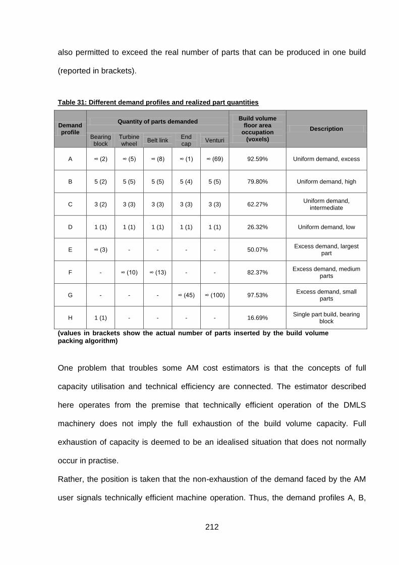
212

also permitted to exceed the real number of parts that can be produced in one build

(reported in brackets).

Table 31: Different demand profiles and realized part quantities

Demand profile

Quantity of parts demanded Build volume

floor area occupation

(voxels)

Description

Bearing block

Turbine wheel

Belt link End cap

Venturi

A ∞ (2) ∞ (5) ∞ (8) ∞ (1) ∞ (69) 92.59% Uniform demand, excess

B 5 (2) 5 (5) 5 (5) 5 (4) 5 (5) 79.80% Uniform demand, high

C 3 (2) 3 (3) 3 (3) 3 (3) 3 (3) 62.27% Uniform demand,

intermediate

D 1 (1) 1 (1) 1 (1) 1 (1) 1 (1) 26.32% Uniform demand, low

E ∞ (3) - - - - 50.07% Excess demand, largest

part

F - ∞ (10) ∞ (13) - - 82.37% Excess demand, medium

parts

G - - - ∞ (45) ∞ (100) 97.53% Excess demand, small

parts

H 1 (1) - - - - 16.69% Single part build, bearing

block

(values in brackets show the actual number of parts inserted by the build volume packing algorithm)

One problem that troubles some AM cost estimators is that the concepts of full

capacity utilisation and technical efficiency are connected. The estimator described

here operates from the premise that technically efficient operation of the DMLS

machinery does not imply the full exhaustion of the build volume capacity. Full

exhaustion of capacity is deemed to be an idealised situation that does not normally

occur in practise.

Rather, the position is taken that the non-exhaustion of the demand faced by the AM

user signals technically efficient machine operation. Thus, the demand profiles A, B,

213

C, E, F and G satisfy the criterion. The rationale is that technically efficient builds

represent minimum cost to the user, not the global minimum cost configuration.

To provide an indication of the actual levels of capacity utilisation resulting from the

execution of the build volume packing algorithm, Table 31 lists the fraction of the build

volume floor voxels that are occupied. It is noteworthy that for the builds deemed to be

technically efficient, this fraction ranges from 50.07% (profile E) to 97.53% (profile G).

A possible criticism of this methodology is the following: by letting the packing

algorithm select parts, the composition of the demand profile changes, eventually

leading to a mismatch with what is demanded by the user. However, the presented

model, based on the instantaneous demand profile dd aims to reflect the situation at a

particular point in time. As discussed in section 3.3.3, adding a temporal dimension

would increase realism but also greatly increase model complexity.

By cumulating the total part volume resulting from builds packed according to each of

the eight demand profiles, summary metrics (per cm³) of comparative process

efficiency can be calculated by the estimation algorithm. Expressed in terms of the

summary metrics of energy consumption (in MJ per cm³) and cost (in £ per cm³) the

results are presented in Figure 70.

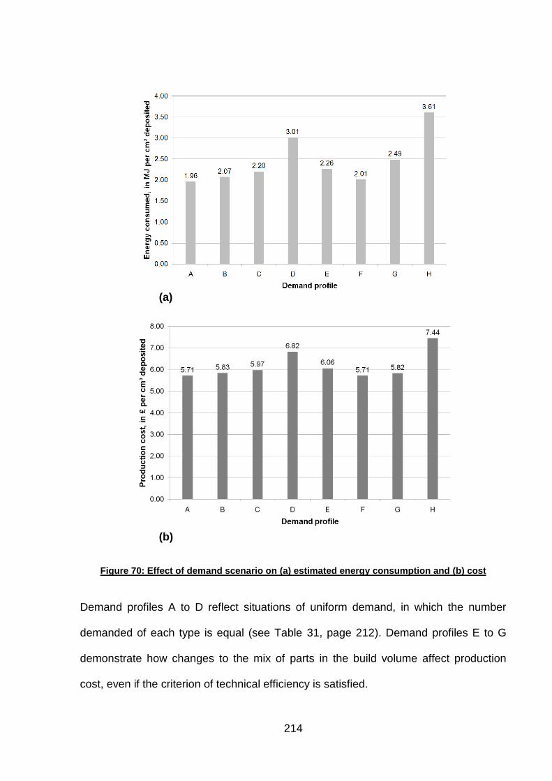
214

(a)

(b)

Figure 70: Effect of demand scenario on (a) estimated energy consumption and (b) cost

Demand profiles A to D reflect situations of uniform demand, in which the number

demanded of each type is equal (see Table 31, page 212). Demand profiles E to G

demonstrate how changes to the mix of parts in the build volume affect production

cost, even if the criterion of technical efficiency is satisfied.

215

The main insight won from the demand profiles A, B and C is that production quantity

is only an indirect determinant of manufacturing cost and energy consumption. The

existing models on the cost of AM, such as Ruffo and Hague (2007), argue that

increases in production quantity diminish average cost by enlarging the allocation

base for the total cost of the build. In contrast, this model shows that the ability to fill

the build volumes drives manufacturing cost.

The results for the other three demand profiles leading to technically efficient builds, E,

F and G, show that changes in the part mix create an unpredictable effect on the

efficiency of the investigated AM process. It appears that some part mixes will

idiosyncratically lead to more efficient builds than others. Ruffo and Hague (2007)

observe the same phenomenon for LS.

In terms of energy consumption, specification A is the most efficient, despite profile G

exhibiting a higher build volume voxel utilisation metric (92.59 % vs. 97.53 %, Table

31). Though not by a wide margin, profile A is also the most cost effective

configuration (570.69 pence per cm³ versus 571.15 pence per cm³ in profile F). This

indicates that builds with a wide variety of parts are likely to lead to improved process

economics through the AM user‟s increased ability to compose builds freely.

7.2.3 Towards a product life cycle view

A central theme in this research is the principle expressed by Waldman (2003) that

durable goods should be viewed as providing a stream of services to users over time.

This shows that the effects and possibilities arising from choosing AM technology, and

in fact any other manufacturing technology, should be analysed according to the

various stages of the product life cycle, for example in the PAS2050:2011 life

framework (British Standards Institution, 2011, as shown in Figure 13, page 46).

216

This is especially important for AM as the benefits of manufacturing complex and

lightweight products are likely to manifest themselves „upstream‟ in the raw material

production stage of the product life cycle and „downstream‟ during the part‟s use

phase.

To the end users, the cost savings resulting from smaller raw material requirements

during manufacturing may seem irrelevant as this information should already be

factored into the purchase price. However, due to the increasing scarcity of natural

resources there is reason to believe that users of durable goods will need to directly

consider such aspects in the future. As argued in the introduction, there are significant

social costs attached to pollution resulting from the environmental footprint in raw

material generation. As these social costs are not measurable, they may be large and

hidden to decision makers further „downstream‟ in the supply chain. The adoption of

AM may be advantageous by minimising waste streams resulting from raw material

usage and, due to the simplicity in its supply chain, enable an unprecedented degree

of transparency of the inputs to production.

Especially if energy intensive raw materials such as titanium are used, the energy

consumed during the raw material generation stage may far surpass the energy

consumed during the manufacturing stage. The following example illustrates this issue

by constructing a comparison of the energy consumed during the raw material

generation and manufacture of a titanium test part (as shown in Figure 20, page 88)

using the EBM process and a conventional CNC route.

It is demonstrated that the energy consumption (and hence social cost) consequences

of process selection resulting from the raw material stage in the product life cycle can

be significant.

217

Combining data on the energy embedded in the raw material with EBM (measured)

and CNC (estimated) process energy consumption, a comparison between the total

energy requirements of the two substitute processes can be assembled (Table 32).

The same approach has been taken by Morrow et al. (2007) in his comparison of the

energy consumed for the production of tool steel inserts by CNC machining and AM

technology variant DMD. The results reached by Morrow et al. (2007) were also cited

by Gutowski et al. (2009) to support the claim that DMD is an energy intensive

process. For this analysis to be reflective of efficient technology usage, the AM energy

consumption metrics are based on the results of the full build experiment on the EBM

platform (identified by the code A08).

CNC energy consumption is estimated synthetically by obtaining upper and lower

bounds of specific energy consumption from the literature for the rough milling / CNC

turning of steel materials. This suggests a specific energy consumption between 24.00

MJ (Morrow et al., 2007) and 6.53 MJ (Steiner and Frischknecht, 2007) per kg

removed. Correspondingly, two summary metrics for total CNC machining energy

consumption are presented below.

For an estimate of the energy investment required for a CNC machined part

(equivalent to the power monitoring geometry shown in Figure 20, page 88) this study

assumes that the part is machined from a plate of Ti-6Al-4V raw material in the size of

the part‟s bounding box (75 × 75 × 24 mm).

The resulting ratio of raw material input mass to post-process part weight (referred to

as the „buy-to-fly‟ ratio) is 4.58, which suggests a relatively modest process energy

consumption and raw material requirement for CNC.

218

Table 32: Total energy consumption per part

Additive Manufacturing pathway

Raw material

Type Ti-6Al-4V powder

Embedded energy per kg of raw material (powder,

Granta Design Ltd., 2010) 560.60 MJ

Raw material input mass 130.61 g

Buy-to-fly ratio 1

Raw material embedded energy 73.22 MJ

EBM Process

Part mass 130.61 g

Amount of material deposited 130.61 g

Specific energy consumption (measured) per kg of

material deposited 59.96 MJ / kg deposited

Amount of material removed None

Process energy consumption pert part 7.83 MJ

Total energy consumption per part 81.05 MJ

CNC machining pathway

Raw material

Type Ti-6Al-4V plate

Embedded energy per kg of raw material (plate,

Granta Design Ltd., 2010) 528.90 MJ

Raw material input mass 598.05 g

Buy-to-fly ratio 4.58

Raw material embedded energy 316.31 MJ

CNC

machining

Process

Part mass 130.61 g

Amount of material removed 467.44 g

Specific energy consumption per kg of material

removed, upper bound (Morrow et al., 2007) 24.00 MJ / kg removed

Specific energy consumption per kg of material

removed, lower bound (Steiner and Frischknecht,

2007)

6.53 MJ / kg removed

Amount of material deposited None

Process energy consumption pert part (upper bound) 11.22 MJ

Process energy consumption pert part (lower bound) 3.05 MJ

Total energy consumption per part (upper bound) 327.53 MJ

Total energy consumption per part (lower bound) 319.36 MJ

The raw material energy requirement is estimated by multiplying the raw material input

requirement (in plate or powder form) by the energy embedded per kg, which results

219

in a total raw material energy estimate of 73.22 MJ for the EBM pathway and 316.31

MJ for the CNC route.

It is noteworthy that the embedded energy per kg of powder material appears only

slightly higher than that of plate material (560.60 MJ/kg compared to 528.90 MJ/kg).

This is caused by the large amounts of energy needed to extract titanium metal from

its minerals (rutile and ilmenite concentrates). The energy needed for the atomisation

process to create powder from the plate feedstock is significant (>30 MJ/kg).

Pure process energy consumption can be obtained by applying the specific energy for

the deposition (EBM) or removal (CNC) of material to the component mass. Thus, for

EBM the total energy consumption per part (with start up, preheating and cool down

factored in through the specific energy per kg deposited) can be expressed as:

( ) (30)

Correspondingly, for the CNC route:

(31)

In the comparison of total energy consumption per part, the EBM route compares very

favourably to the conventional CNC manufacturing route (81.05 MJ versus 319.36 to

327.53 MJ). This result is further supported by the moderate buy-fly-ratio exhibited in

the CNC pathway. In both techniques, total energy usage is dominated by the energy

embedded in the raw material.

220

The energy consumption levels presented in Table 32 contrast the result reached by

Morrow et al. (2007) reporting specific energy consumption for the additive technology

variant DMD (7708 MJ per kg deposited), leading to process energy consumption far

outweighing the energy embedded in the raw material.

The high specific energy consumption reported by Morrow et al. may be the result of a

slow deposition rate setting in the experimental setup described by Morrow et al. In

terms of additive techniques, DMD is also different to the processes assessed in this

work. It may therefore consume more energy. Further complicating matters, the

experimental data provided by Morrow et al. include a heat treatment procedure and

are based on a far less energy intensive raw material (H13 tool steel).

Table 32 indicates that the specific energy consumption for the additive pathway may

be higher than for the conventional route. For the EBM process, 59.96 MJ per kg

deposited are measured, this compares to 6.53 MJ to 24.00 MJ per kg removed for

the CNC pathway.

Due to the fundamental difference in operating principle, however, this result is not

very meaningful. It does nevertheless indicate that CNC is at a disadvantage in terms

of energy efficiency in this particular case as subtractive processes are not able to

produce final geometries from cuboid raw material without creating significant waste

streams. It should be noted that this analysis concentrates purely on the energy and

raw material inputs to manufacturing: ancillary inputs, such as lubricants and

pressurised air, are not considered.

According to the „waste hierarchy‟ literature (see, for example, Barrett and Lawlor,

1997), there are several available options in waste management: disposal, energy

recovery (incineration), recycling, re-use, and prevention. These strategies are ranked

according to their desirability, as shown in Figure 71. In the waste hierarchy, the

221

prevention of waste streams through (for example through EBM adoption) is classed

as a highly desirable outcome.

Figure 71: Waste mitigation through EBM adoption in the waste hierarchy

Image source: own work

Furthermore, it has been argued above that for CNC produced parts, there is a

connection between part design and energy consumption. According to Avram and

Xirouchakis (2011), the various milling techniques used to realise geometric features

exhibit differences in specific energy consumption. Further it is argued that a large

component of CNC energy consumption is attributable to machine idleness during

build programmes, for example occurring during tool changes. This suggests that the

CNC manufacture of more complex, and arguably more functional, component

geometries will come at an increased process energy cost (as well as higher

wastage). Concerning EBM, empirical evidence is presented in this thesis that shape

complexity is only weakly related to energy consumption.

A key argument brought forward by Lovins (1996) is that private incentives need to be

aligned correctly for energy efficiency gains to be realised, such that cost reductions

coincide with energy savings. This argument is extensible to life cycle assessment for

durable goods. As noted by Murr et al. (2009), machining complex titanium parts from

222

mill products is financially expensive. For titanium parts produced via CNC, there is

thus a monetary cost incentive to keep deviation from the shape of the mill product to

a minimum. This may result in non-minimal production-phase energy consumption

during CNC milling operations. Rajemi et al. (2010) have noted in this context that the

minimum cost configuration does not necessarily meet the criterion of minimum

energy consumption in CNC.

Taking into account energy consumed for raw material generation, the presented data

indicate that the EBM route consumes roughly one quarter of the energy used by its

conventional CNC counterpart. This large discrepancy arises mainly from the absence

of waste streams occurring in the CNC route. However, it must be stressed that

additional surface quality improvement and heat treatment procedures may be

necessary for the EBM output; these extra process steps may not be required for

milled products.

Despite efforts to include environmental and social considerations in engineering

decisions (Maxwell and Van der Vorst, 2003), private costs and benefits (accruing to

individuals and organisations, as opposed to society) are normally viewed as the

determinants of technology adoption decisions (Stoneman, 2002). In many part

applications (transportation in particular), intricate and light weight components may

enable significant cost and energy savings (Helms and Lambrecht, 2007). Therefore,

manufacturing cost minimisation in CNC may also be at odds with use-phase

efficiency, both in terms of energy consumed during the part‟s use phase as well as in

terms of operating cost.

In the context of transportation applications, the existing relationships between

operating cost savings resulting from reduced part weight may be structured by

applying the concept of „elasticity‟.

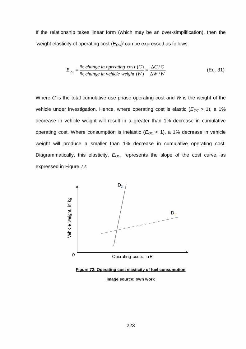
223

If the relationship takes linear form (which may be an over-simplification), then the

„weight elasticity of operating cost (EOC)‟ can be expressed as follows:

WW

CC

Wweightvehicleinchange

CtoperatinginchangeEOC

/

/

)(%

)(cos%

(Eq. 31)

Where C is the total cumulative use-phase operating cost and W is the weight of the

vehicle under investigation. Hence, where operating cost is elastic (EOC > 1), a 1%

decrease in vehicle weight will result in a greater than 1% decrease in cumulative

operating cost. Where consumption is inelastic (EOC < 1), a 1% decrease in vehicle

weight will produce a smaller than 1% decrease in cumulative operating cost.

Diagrammatically, this elasticity, EOC, represents the slope of the cost curve, as

expressed in Figure 72:

Figure 72: Operating cost elasticity of fuel consumption

Image source: own work

224

As introduced above, D1 represents the case of a vehicle design with a high weight

elasticity of operating cost, for example in aviation applications where fuel

consumption is very sensitive to aircraft weight (Helms and Lambrecht, 2006).

In this case, minor reductions in vehicle weight will produce significant cumulative

savings in the use phase operating cost and energy consumption. Advanced, light-

weight designs could be viable because increases in manufacturing cost may be offset

by later savings in operating cost. In the opposite case, represented by D2, the

chances for this to happen are lower; the costs incurred during the use-phase are not

as sensitive to vehicle weight.

225

Chapter 8: Conclusions

This thesis concludes by summarising the results reached and attempts to fit them into

the broader context. Following this chapter, this thesis ends with recommendations for

further research activity and suggestions on how the results could be exploited in a

commercial setting.

Regarding the existing body of literature on the economic evaluation of technology,

Souder and Shrivastava (1985) note that we “can't begin to make decisions about

"technology" until we understand it. And we can't begin to really understand it until we

can measure it.”

To measure the „economics‟ of AM, this thesis has presented a systematic analysis of

the benefits and costs arising from the adoption of additive production systems. The

three research goals spelled out in section 1.2 have been addressed as follows:

I. A methodology for the measurement of shape complexity as a visibility metric

has been developed and implemented. Concerning the process energy inputs

to the EBM process, the results discussed in chapter 7 indicate that energy

consumption and shape complexity are unrelated. However, due to the narrow

analytical approach, it was not demonstrated that complexity is free in terms of

build time and manufacturing cost. Moreover, the results are applicable only to

EBM (and possibly other powder bed fusion processes).

II. Chapter 5 has reported reliable empirical summary data on the productivity of

various major AM technology variant. It is shown that operating the systems at

full capacity promotes productivity. The importance of this varies according to

the technology type, however. Chapter 6 has reported corresponding summary

metrics for AM energy consumption. The pattern is repeated: for all platforms

226

increased capacity utilisation results in smaller specific process energy

consumption. However, the impact of capacity utilisation on platform efficiency

varies across platforms. While the benefit of the exploitation of available build

space is relatively small for FDM, the same benefit is very large for the

analysed polymeric LS platform.

III. The methodology used in to address objective II has also been used to

generate data for the ex-ante estimation of build time, energy consumption and

cost. This combined estimator has been implemented and validated for the

EOSINT M270 DMLS platform. The resulting tool is designed to handle the

multi-part and multi-product case typically (and exclusively) found in AM

applications. In chapter 7 it has been argued that the AM user‟s ability to fill the

available build space with parts is the key determinant of efficient AM

technology operation.

Next to addressing the primary research goals, it has been demonstrated that the one-

stop nature of AM enables the accurate estimation of monetary and energy costs even

for complex products. This an important step in the inventory element of studies of life

cycle energy consumption.

This thesis has thus shown that AM‟s ability to create complex geometry and its

parallel nature both shape the associated process economics and dictate efficient

technology usage. Going back to the Gershenfeld‟s (2007) comment from Chapter 1,

stating that “we don‟t need to keep having [the digital revolution]”, the acceptance of

these (probably novel) economic aspects for manufacturing technology may lead to a

timely exploitation of AM‟s potential and the appropriate technology diffusion path.

227

8.1 Contextualisation of results

Guiding the analysis throughout this thesis, Tuck et al. (2008) suggests that AM

possesses two advantages over other, more conventional manufacturing techniques.

Firstly, AM is able to efficiently generate geometrically complex components; and

secondly, the technology is able to produce very small production quantities at a

relatively low average cost.

This research has demonstrated a methodology for the quantification of measures

associated with complexity. Using a measure reflecting shape complexity, as

proposed by Psarra and Grajewski (2001), it has been shown that the energy inputs to

the AM variant EBM do not correlate with the complexity found in the layers of a test

part. This gives reason to believe that in some AM processes, such as EBM, the

financial production cost will also be independent of product complexity. As noted by

Hague et al. (2003), this is a novel feature for manufacturing processes and is unlike

most conventional processes.

Contributing to the on-going debate on AM‟s ability to efficiently manufacture products

in low volumes (down to a single unit), this research has discussed the determinants

of energy consumption and financial production cost. In terms of pure process energy

consumption, it is demonstrated that the degree of capacity utilisation is highly

important for summary metrics of energy consumption on some platforms. The

presented evidence reveals that especially powder bed fusion AM technology, such as

LS, SLM, DMLS and EBM are subject to severe economic penalties if the available

build volume capacity is not fully used. On the other hand, the economics of the FDM

process appear to be relatively independent of the degree of build volume capacity

utilisation.

228

Overall levels of specific energy consumption were measured using a consistent

methodology for major AM technology variants. In the experimental set up that should

be reflective of AM technology usage in practise, the measured specific energy

consumption ranges from 59.96 MJ per kg (Arcam A1) to 519.47 MJ per kg of material

deposited (Stratasys FDM400mc).

As shown conclusively by the combined energy consumption and cost model built

around data from the EOSINT M270 DMLS system, build volume utilisation is a major

determinant of both process energy consumption and financial production cost. This is

relatively similar to the intuition behind the existing models of AM manufacturing cost

(Ruffo et al., 2006b; Munguia, 2009; Wilson, 2009), where empty build volume

capacity drives up the reported manufacturing cost.

However, unlike some previous models of manufacturing cost, this thesis argues that

is not possible to infer a relationship between manufacturing unit cost and production

quantity. The reason for this is that the underlying behaviour would not be rational. In

reality, empty capacity is avoided by the users of AM systems (Ruffo and Hague,

2007). This can be achieved by postponing builds, selling excess capacity to external

demanders or adopting a smaller AM system.

Thus, this thesis suggests that the AM users‟ ability to fill the available machine

capacity is the linchpin for favourable manufacturing economics on most AM

platforms, apparently with the exception of FDM.

Motivated by the need to reduce the energy consumption associated with the

manufacture and use of durable goods, there is an increased tendency to take into

account the whole life cycle in engineering design. This thesis appreciates that the

environmental impact of durable goods is not restricted to the production processes. It

extends „upstream‟ to the raw material generation process and „downstream‟ to the

229

product‟s use-phase and to its disposal. Here, the adoption of AM may be beneficial in

two ways: due to its ability to create complex products in a single step the wastage of

raw material is minimised. Moreover, its ability to fully differentiate products to the

function they will perform during their use phase should ultimately result in highly

effective and functional products. These gains may be large enough to compensate

for disadvantages in terms of manufacturing cost or manufacturing energy

consumption.

According to Stoneman (1995), an important research puzzle deals with the issue of

whether environmentally benign technologies may be privately profitable. The

evidence presented in this thesis, especially the outcomes of the combined energy

consumption and cost model, points to the conclusion that the minimum cost

configuration in AM is also the configuration that minimises the energy inputs during

the manufacturing stage.

Hence, from an ecological standpoint, AM adoption may come with the side-effect of

correcting production configurations with non-minimal energy inputs. This aspect may

be an important prerequisite for energy efficiency gains in manufacturing (Lovins,

1996). Moreover, a corrective of this kind is perhaps also a hallmark of a particular

class of technology described as „Mumfordian biotechnics‟. It has been argued that

these technologies may in the distant future replace conventional mass production by

a more benign, scalable and product performance oriented manufacturing approach

(Mumford, 1971). Aspects of AM that support this classification are the qualitative

richness of products enabled by AM (Hollington, 2008) and the freedom from

quantitative pressures associated with the absence of sunk tooling costs present in

traditional mass production (Ruffo et al., 2006b).

230

Chapter 9: Recommendations for further work

Ending this thesis, recommendations for further work are made. Importantly, some

results reached in this thesis are directly applicable to software products incorporating

cost and energy consumption estimation functionality. Thus the recommendations for

further work are split up into the starting points for further research and applications

that may have commercial promise.

9.1 Further research

The combined build time, energy consumption and cost estimation methodology

developed in this research is able to generate consistent and reliable estimates for AM

processes with internal build volumes. This thesis has applied this methodology only

to the EOSINT M270 DMLS system, resulting in cost estimates of £5.71 to £6.06 per

cm³ and specific energy consumption estimates ranging from 1.96 MJ to 2.49 MJ per

cm³ deposited. Given appropriate data, the model can also be applied to other AM

processes, including those allowing full 3D build arrangements, like LS.

However, as this research has argued, for a truly accurate reflection of the build

volume packing problem, the AM user may have to consider a stream of available

builds on multiple machines, resulting in a highly complex, multi-machine, multi-period

build volume packing problem.

Moreover, the estimator can be used to learn about the effect of incremental

improvements in system performance. Resembling a sensitivity analysis, this

approach could explore the effect of, for example, a 10% improvement in build speed,

or a 10% increase in energy efficiency. This would shed some light on the impact of

231

near future technology improvements on AM process economics, perhaps resulting in

increased technology diffusion speed.

The work towards research objectives II and III has shown (at least for the DMLS

platform) that dense packing configurations lead both to manufacturing cost

minimisation and to process energy consumption minimisation. The driver of efficient

technology operation appears to be the user‟s ability to fill the available build volumes

effectively with parts. It has not been explored if full capacity utilisation affects part

accuracy, surface quality or mechanical properties.

However, the result that for efficient technology operation the available capacity

should be utilized may impact on-going research for „Design for AM‟ methodologies,

with the objectives of cost and process energy consumption minimisation. This result

could also lead to more realistic estimators of AM performance. Additional progress in

this area may be relevant to the designers of additive machinery, which could help in

the development of a new generation of more efficient manufacturing technology. For

example, the build envelopes of AM systems could be shaped and sized based on

empirical and statistical work with AM technology adopters. Another, more immediate

area of research would be the scope for improvement for thermal management on

additive platforms. The results presented in this thesis indicate that dramatic

improvements in specific energy consumption could be achieved by modifying

machine insulation and, particularly, cooling.

The result that the ability to fill build volumes efficiently (as opposed to production

quantity) is the key determinant for process efficiency is of relevance to AM

practitioners. By pooling orders, and thus creating a situation of fungible demand, AM

users may able maximise process efficiency. Such network effects are a characteristic

of general purpose technology, as defined by Bresnahan and Trajtenberg (1996).

232

Moreover, existing technology adopters may not fully exploit AM‟s capability to create

differentiated and functionally optimised products. The reason for this may however be

the shortcomings of currently available 3D CAD software. An increased ability to

design more complex parts and products, perhaps closer to some platonic „ideal

configuration‟, may also make AM a more attractive proposition.

9.2 Commercialisation considerations

This thesis has shown how build time, energy consumption and cost estimates can be

generated for builds that are populated with parts drawn from a basket of

representative components. The same approach is also useful in the determination of

AM production cost for new designs by filling the void areas with some representative

parts.

It appears that this is a valid approach to cost modelling for parallel manufacturing

systems if the composition of the production build is unknown. Furthermore, the

composition of the build simulated in the presented methodology (via the part

precedence vector p and the instantaneous demand profile dd) can be adapted to a

particular business situation. Thus, the cost and energy consumption estimates can be

tailored to the individual user. Using this technique, it would be possible to produce

more accurate estimates for firms that, for example, produce predominantly small

parts.

Besides improving the accuracy of estimates of well-structured cost (as defined by

Son, 1991) this approach could add some value to the available software products

with cost estimation functionality. Moreover, being a single-step, electricity driven

manufacturing approach, AM allows the estimation of credible process energy

233

consumption figures. This ability could prove extremely valuable where information on

embodied energy needs to be communicated to the consumer.

The process energy consumption summary metrics produced in this research are

already used in a commercial implementation that benchmarks the environmental

impact of manufacturing supply chains (‟Enlighten‟, Econolyst Ltd. and Kinetic ICT

Solutions Ltd., 2011).

234

References

1. 3D Systems Corporation, 2011. Corporate website [Online]. Available

from: production3dprinters.com [Accessed: 22.09.2011.]

2. Alexander, P., Allen, S., and Dutta, D., 1998. Part orientation and build cost determination in layered manufacturing. Computer-Aided Design, 30 (5), pp. 343-356.

3. Anderson, C. 2006. The Long Tail: Why the Future of Business Is Selling Less of More. New York: Hyperion Books.

4. Arcam AB, 2010. Arcam A1 – The future in implant manufacturing. [Online]. Available from: http://www.arcam.com/CommonResources/Files/www.arcam.com/Documents/Products/Arcam-A1.pdf [Accessed: 15.06.2010]

5. ASTM, 2012. ASTM F2792 - 12e1 Standard Terminology for Additive

Manufacturing Technologies. [Online]. Available from: www.astm.org/Standards/F2792.htm [Accessed: 04.10.2010].

6. ATKINS feasibility study. Downloads, 2008. [Online]. Available from: http://atkins-project.com/web/atkins/pdf/ATKINSfeasibilitystudy.pdf [Accessed: 28.01.2009]

7. Atrill, P., and McLaney, E., 1999. Management Accounting for Decision Makers. 2nd ed. London: Prentice Hall Europe.

8. Avison, W., and Nettler, G., 1976. World Views and Crystal Balls. Futures.

8 (1), pp. 413-414.

9. Avram, O. I., and Xirouchakis, P., 2011. Evaluating the use phase energy

requirements of a machine tool system. Journal of Cleaner Production, 19

(6-7), pp. 699-711.

10. Barrett, A., and Lawlor, J., 1997. Questioning the Waste Hierarchy: The

Case of a Region with a Low Population Density. Journal of Environmental

Planning and Management, 40 (1), pp. 19-36.

11. Baumers, M., Tuck, C., Hague, R., Ashcroft, I., and Wildman, R., 2010. A comparative study of metallic additive manufacturing power consumption. Proceedings of the Solid Freeform Fabrication (SFF) Symposium. The University of Texas at Austin, 2010.

12. Baumers, M., Tuck, C., Hague, R., 2011a. Realised levels of geometric complexity in additive manufacturing. International Journal of Product Development, 13 (3), pp.185–203.

235

13. Baumers M., Tuck, C., Bourell, D., Sreenivasan, R., Hague, R., 2011b. Sustainability of additive manufacturing: measuring the energy consumption of the laser sintering process. Proceedings of the Institution of Mechanical Engineers Part B: Journal of Engineering Manufacture. 225 (12), pp. 2228-2239.

14. Baumers, M., Tuck, C., Wildman, R., Ashcroft, I., and Hague, R., 2011c.

Energy inputs to additive manufacturing: does capacity utilization matter? Proceedings of the Solid Freeform Fabrication (SFF) Symposium. The University of Texas at Austin, 2011.

15. Baumers, M., Tuck, C., Wildman, R., Ashcroft, I., Rosamond, E., Hague, R., forthcoming. Transparency built-in: energy consumption and cost estimation for additive manufacturing. Manuscript resubmitted after major revision on 25.01.2012 to the Journal of Industrial Ecology.

16. Bergmann, F., 2004. Neue Arbeit, Neue Kultur (New work, New Culture).

Freiamt: Arbor Verlag.

17. Bernst, R., 1975. Werkstoffe im wissenschaftlichen Gerätebau (Materials in Scientific Mechanical Engieering). Leipzig: Akademische Verlagsgesellschaft Geest & Portig.

18. Boothroyd, G., Dewhurst, P., and Knight, W., 1994. Product Design for Manufacture and Assembly. New York; Marcel Dekker.

19. Bralla, J., 1998. General design principles for manufacturability. In J. Bralla, ed. Design For Manufacturability Handbook. New York: McGraw-Hill.

20. Bresnahan, T. F., and Trajtenberg, M., 1996. General Purpose Technologies: ‚Engines of Growth?‟. Journal of Econometrics, Annals of Econometrics 65, pp.83-108.

21. British Standards Institution, 2011. PAS 2050, Guide to., Energy, PAS

2050, 2011. [Online]. Available from: http://www.bsigroup.com/en/Standards-and-Publications/Industry-Sectors/Energy/PAS-2050 [Accessed: 15.05.2009]

22. Bulow, J., 1982. Durable Goods Monopolists. Journal of Political Economy. 90/2, pp.314-332.

23. Burns, M., 1993. The Household Fabricator. Comments offered in Panel Discussion on Future Directions in Solid Freeform Fabrication at [the] Fourth Solid Freeform Fabrication Symposium University of Texas at Austin, Austin, Texas, August 11, 1993 [Online]. Available from: www.ennex.com/~fabbers/publish/199308-MB-HouseholdFab.asp [Accessed: 01.09.2011].

236

24. Byun, H., Lee, K. H., 2006. Determination of the optimal build direction for different rapid prototyping processes using multi-criterion decision making. Robotics and Computer-Integrated Manufacturing, 22 (1), pp.69-80.

25. Cabral, L. M. B., 2000. Introduction to Industrial Organization. London: MIT Press.

26. Campbell, I., Combrinck, J., De Beer, D., and Barnard, L., 2008. Stereolithography build time estimation based on volumetric calculations. Rapid Protoyping Journal, 14 (5), pp. 271-279.

27. Chahine, G., Koike, M., Okabe, T., Smith, P., Kovacevic, R., 2008. The Design and Production of Ti-6Al-4V ELI Customized Dental Implants. JOM Journal of the Minerals, Metals and Materials Society. 60 (11), pp. 50-55.

28. Castle Island Co., 2011. The Most Important Commercial Rapid Prototyping Technologies at a Glance. [Online]. Available from: www.additive3d.com/rp_int1.htm [Accessed: 20.09.2011]

29. Chen, C., and Sullivan, P. A., 1996. Predicting total build-time and the resultant cure depth of the 3D Stereolithography process. Rapid Prototyping Journal, 2 (4), pp. 27-40.

30. Cheng, W., Fuh, J. Y. H., Nee, A. Y. C., Wong, Y. S., Loh, H. T. and Miyazawa T., 1995. Multi-objective optimization of part-building orientation in stereolithography. Rapid Prototyping Journal, 1 (4), pp.12–23.

31. Choi, S. H., and Samavedam, S., 2002. Modelling and optimisation of rapid prototyping. Computers in Industry, 47 (1), pp. 39-53.

32. Christensen, P. W., and Klarbring, A., 2009. An Introduction to Structural Optimization. 1st ed. Hamburg: Springer.

33. Coccia, M., 2004. Measuring intensity of technological change: The seismic approach. Technological Forecasting & Social Change, 72/1, pp.117-144.

34. ConceptLaser GmbH, 2011. Corporate website [Online]. Available from: http://www.concept-laser.de/ [Accessed: 01.07.2011].

35. ConceptLaser GmbH, 2007. My name is M3. M3 Linear. [Online]. Available from: http://www.estechnology.co.uk/images/m1m2m3/m3linear.pdf [Accessed: 01.08.2012].

36. Cormier, D., West, H., Harryson, O., and Knowlson, K., 2004a. Characterization of thin walled Ti-6Al-4V components produced via electron beam melting. Proceedings of the 15th Solid Freeform Fabrication Symposium, Austin, USA.

237

37. Cormier, D., Harryson, O., and West, H., 2004b. Characterization of H13 steel produced via electron beam melting. Rapid Prototyping Journal, 10 (1), pp. 35-41.

38. DECC, 2010. Quarterly energy prices, December 2010. [Online]. Available

from: http://www.decc.gov.uk/assets/decc/Statistics/publications/prices/1085-qepdec10.pdf [Accessed: 10.05.2011].

39. Di Angelo, L., Di Stefano, P., 2011. A neural network-based build time estimator for layer manufactured objects. The International Journal of Advanced Manufacturing Technology, DOI: 10.1007/s00170-011-3284-8

40. Dodson, E. N., 1985. Measurement of State of the Art and Technological Advance. Technological Forecasting and Social Change 27, pp.129-146.

41. Dreyfus, M., and Viscusi, W. K., 1995. Rates of time preference and consumer valuations of automobile safety and fuel efficiency. Journal of Law and Economics. 38(1), pp.79-105.

42. Econolyst Ltd. and Kinetic ICT Solutions Ltd., 2011. Corporate website [2011]. Available at: http://www.enlighten-toolkit.com/ [Accessed: 08.10.2011].

43. Edmonds, B., 1999. What is Complexity? - The philosophy of complexity per se with application to some examples in evolution. In F. Heylighen and D. Aerts, eds. The Evolution of Complexity. Kluwer: Dordrecht.

44. Else, P., and Curwen, P., 1990. Principles of Microeconomics. London: Unwin-Hyman.

45. EOS GmbH, 2010. Corporate website [Online]. Available from: www.eos.info/en/products.html [Accessed: 24.09.2010].

46. Fabberhouse, 2011. Corporate website [Online]. Available from: www.alphacam.de/fabberhouse/start [Accessed: 20.09.2011].

47. FedEx, 2008. [Online]. Press Release / FedEx Spotlight. Available from: news.van.fedex.com/fedex_office [Accessed: 01.09.2011].

48. Fisher, M., 1997. What is the right supply chain for your product? Harvard Business Review. 75(2), pp.105-116.

49. Flusser, V., 1999. The Shape of Things: A Philosophy of Design. London: Reaktion Books.

50. Foran, B., Lenzen, M., Dey, C., and Bilek, M., 2005. Integrating sustainable chain management with triple bottom line accounting. Ecological Economics, 52 (2), pp. 143-157.

238

51. Forbes, 1978. The Future That Never Came. Forbes Magazine, 122, July 10, 1978. pp.51-52.

52. Friebe, H., and Ramge, T., 2008. Marke Eigenbau – Der Aufstand der Massen gegen die Massenproduktion (Brand Self-Constructed – The Revolution of the Masses Against Mass Production). Frankfurt: Campus.

53. Gebhardt, A., 2008. Generative Fertigungsverfahren (Additive Manufacturing Processes). 3rd ed. Munich: Carl Hanser Verlag.

54. Gershenfeld, N., 2005. Fab – The Coming Revolution on Your Desktop-from Personal Computers to Personal Fabrication. New York: Basic Books.

55. Gershenfeld, N., 2007. [Online] Neil Gershenfeld on Fab Labs. TED talks. Available at: http://www.ted.com/talks/lang/en/neil_gershenfeld_on_fab_labs.html [Accessed 02.11.2011].

56. Giannatsis, J., Dedoussis, V., and Laois, L., 2001. A study of the build-time estimation problem for stereolithography systems. Robotics and Computer Integrated Manufacturing, 17 (1), pp. 295-204.

57. Gibson, I., Rosen, D., Stucker, B., 2010. Additive Manufacturing Technologies – Rapid Prototyping to Direct Digital Manufacturing. New York: Springer.

58. Gößling-Reisemann, S., 2008. What Is Resource Consumption and How Can It Be Measured? Theoretical Considerations. Journal of Industrial Ecology, 12 (1), pp. 10-25.

59. Granta Design, 2010. [Online] Corporate Website. Available at: http://www.grantadesign.com/education/ [Accessed 13.12.2010].

60. Griliches, Z., 1957. Hybrid Corn: An Exploration in the Economics of Technological Change. Econometrica, 25/1, pp.501-522.

61. Griliches, Z., 1987. Productivity: Measurement Problems. In J. Eatwell, M. Milgate, and P. Newman, eds. The New Palgrave Dictionary of Economics. London: Macmillan.

62. Grupp, H., and Hohmeyer, O., 1986. A Technometric Model for the Assessment of Technological Standards and Their Application to Selected Technology-Intensive Products. Technological Forecasting and Social Change, 30, pp.123-137.

239

63. Gutowski, T. G., Branham, M. S., Dahmus, J. B., Jones, A. J., Thiriez, A., and Sekulic, D. P., 2009. Thermodynamic Analysis of Resources Used in Manufacturing Processes. Environmental Science and Technology, 43 (5), 1584-1590.

64. Hague, R., Campbell, I., and Dickens, P., 2003. Implications on design of rapid manufacturing. Proceedings of IMechE Part C: Journal of Mechanical Engineering Science, Vol. 217, No. C1, 25-30.

65. Hague, R., 2004. [Online] A skills needs analysis for the engineering sector in Derbyshire, 9: the future engineering economy. Available from: http://www.econolyst.co.uk/pdf/publications/December%202004%20-%20Forecasting%20the%20future%20engineering%20skills%20needs%20of%20Derbyshire%20employers.pdf [Accessed: 13.02.2011].

66. Hague R., Mansour, S., and Saleh, N., 2004. Material and design considerations for rapid manufacturing. International Journal of Production Research, 42 (22), pp. 4691-4708.

67. Hall, B. H., 2005. Innovation and Diffusion. In J. Fagerberg, D. C. Mowery and Nelson, R. R., eds. The Oxford Handbook of Innovation. Oxford: University Press. Ch. 17.

68. Harrysson, O., Deaton, B., Bardin, J., West, H., Cansizoglu, O., Cormier, D., Marcellin-Little, D., 2005. Evaluation of titanium Implant Components Directly Fabricated Through Electron Beam Melting Technology. Proceedings of the Materials & Processes for Medical Devices Conference, 2005, Boston, USA.

69. Held, M., and Pfligersdorffer, C. Correcting warpage of laser-sintered parts by means of a surface base inverse deformation algorithm. Engineering with Computers, 2009, 25 (1), pp. 389-395.

70. Hein, P., 1934. [Online] Patent specification for the Soma cube, No. 420,349. Available from: http://www.fam-bundgaard.dk/SOMA/NEWS/N030310.HTM [Accessed: 22.02.2012]

71. Helms, H., and Lambrecht, U., 2006. [Online] The Potential Contribution of Light Weighting to Reduce Transport Energy Consumption. International Journal of Life-Cycle Assessment. Available from: http://www.ifeu.de/verkehrundumwelt/pdf/Helms(2006)_light-weighting.pdf [Accessed: 13.03.2009]

72. Herzog, T., 2009. [Online] World greenhouse Gas Emissions in 2005. Available from: http://pdf.wri.org/working_papers/world_greenhouse_gas_emissions_2005.pdf [Accessed: 15.07.2011].

240

73. Hollington, G., 2008. [Online] Design 2.0. TCT Conference Archive. Available at http://www.tctmagazine.com/library/115/Design%202.0.pdf [Accessed 18.05.2011].

74. Hopkinson, N., and Dickens, P., 2003. Analysis of rapid manufacturing - using layer manufacturing processes for production. Proceedings of the Institution of Mechanical Engineers, Part C: Journal of Mechanical Engineering Science. 217 (C1), pp. 31-39.

75. Hopkinson, N., and Dickens, P. M., 2006. Emerging Rapid Manufacturing Processes. In N. Hopkinson, R. J. M. Hague, and P. M. Dickens, eds. Rapid Manufacturing – An Industrial Revolution for the Digital Age. Chichester: Wiley. Ch. 5.

76. Hotelling, H., 1929. Stability in Competition. Economic Journal. 39 (153), pp.41-57.

77. Hoy, M., Livernois, J., McKenna, C., Rees, R., and Stengos, T., 2001. Mathematics for Economics. 2nd ed. Cambridge: MIT Press.

78. Hur, S., Choi, K., Lee, S., Chang, P., 2001. Determination of fabricating oriantation and packing in SLS process. Journal of Mateials Processing Technology, 112 (1), pp. 236-243.

79. Ikonen, I., Biles, W. E., Kumar, A., Ragade, R. K., Wissel, J. C., 1997. A Genetic Algorithm for Packing Three-Dimensional Non-Convex Objects Having Cavities and Holes. Proceedings of the 7th International FAIM Conference.

80. Jeswiet, J., and Kara, S., 2008. Carbon emissions and CESTM in manufacturing. CIRP Annals – Manufacturing Technology, 57 (1), pp. 17-20.

81. Jiménez-González, C., and Overcash, M., 2000. Energy sub-modules applied in life-cycle inventory of processes. Clean Products and Processes, 2 (1), pp. 57-66.

82. Jovane, F., Yoshikawa, H., Alting, L., Boër, C. R., Westkämper, E.,

Williams, D., Tseng, M., Seliger, G., Paci, A. M., 2008. The incoming global technological and industrial revolution towards competitive sustainable manufacturing. CIRP Annals – Manufacturing Technology, 57 (2), pp. 641-659.

83. Kander, A., 2005. Baumol‟s disease and dematerialization of the Economy. Ecological Economics. 55 (1), pp.119-130.

241

84. Kellens, K., Dewulf, W., Overcash, M., Hauschild, M. and Duflou, J.R.,

2012. Methodology for systematic analysis and improvement of manufacturing unit process life cycle inventory (UPLCI) – CO2PE! initiative (cooperative effort on process emissions in manufacturing). Part 1: Methodology Description. The International Journal of Life Cycle Assessment, 17 (1), pp. 69-78.

85. Kellens, K., Yasa, E., Dewulf, W., and Duflou, J., 2010a. Environmental assessment of selective laser melting and selective laser sintering. Going Green – CARE INNOVATION 2010: From Legal Compliance to Energy-efficient Products and Services. Vienna, Austria.

86. Kellens, K., Dewulf, W., Deprez, W., Yasa, E., and Duflou, J. R., 2010b. Environmental analysis of SLM and SLS in manufacturing processes. Proceedings of the 2010 CIRP International conference on Life Cycle Engineering, Heifei, China.

87. Krugman, P., 1998. [Online]. An Interview with Paul Krugman by Joel Kurtzman. Available at: http://www.strategy-business.com/article/13652?gko=2e802 [Accessed: 04.05.2011]

88. Kulkarni, P., Marsan, A., and Dutta, D., 2000. A review of process planning techniques in layered manufacturing. Rapid prototyping Journal, 6 (1), pp.18-35.

89. Levy, G. N., Schindel, R., Kruth, J. P., 2003. Rapid Manufacturing and Rapid Tooling with Layer Manufacturing (LM) Technologies, State of the Art and Future Perspectives. CIRP Annals – Manufacturing Technology. 52 (2), pp. 589-609.

90. Lovins, A. B., 1996. Negawatts – Twelve transitions, eight improvements and one distraction. Energy Policy, 24 (4), pp.331-343.

91. Luo, Y., Ji, Z., Leu, M. C., and Caudill, R., 1999. Environmental Performance Analysis of Solid Freeform Fabrication Processes. Proceedings of the 1999 IEEE International Symposium on Electronics and the Environment, pp 1-6.

92. Marcam Engineering GmbH, 2012. Corporate Website [Online]. Available from http://www.marcam.de/cms/home.2.html [Accessed 15/05/2012]

93. Martin, S., 2001. Advanced Industrial Economics. 2nd ed. Oxford: Blackwell.

94. Maxwell, D., Van der Vorst, R., 2003. Developing sustainable products and services. Journal of Cleaner Production. 11 (8), 2003. pp.883-895.

242

95. Mazzioli, A., Germani, M., Raffaeli, R., 2009. Direct fabrication through

electron beam melting technology of custom cranial implants designed in a PHANToM-based haptic environment. Materials and Design, 30 (8), pp.3186-3192.

96. Milgrom, P., and Roberts, J., 1995. Complementarities and fit Strategy, structure, and organizational change in manufacturing. Journal of Accounting and Economics. 19(1), pp. 179-208.

97. Mognol, P., Lepicart, D., and Perry, N., 2006. Rapid prototyping: energy and environment in the spotlight. Rapid Prototyping Journal, 12(1), pp. 26-34.

98. Moore, G., 1965. Cramming more components onto integrated circuits. Electronics, Vol.8, April 19.

99. Morrow, W. R., Qi, H., Kim, I., Mazumder, J., and Skerlos, S. J., 2007. Environmental aspects of laser-based and conventional tool and die manufacturing, Journal of Cleaner Production, 15(10), pp. 932-943.

100. Mumford, L., 1971. The Myth of the Machine – The Pentagon of Power. London: Secker & Warburg.

101. Munguia, F. J., 2009. RMADS: Development of a concurrent Rapid Manufacturing Advice System. Ph.D. thesis, Universitat Politecnica de Catalunya, Barcelona, Spain.

102. Murr, L. E., Quinones, S. A., Gaytan, S. M., Lopez, M. I., Rodela, A., Martinez, E. Y., Hernandez, D. H., Martinez, E., Medina, F., Wicker, R. B., 2009. Microstructure and mechanical behaviour of Ti-6Al-4V produced by rapid-layer manufacturing, for biomedical applications. Journal of the mechanical behaviour of biomedical materials, 9 (1), pp. 20-32.

103. NCP Leasing, Inc., Consumables. 2008. [Online]. Available from: http://www.ncpleasing.com/resid/consumables.html [Accessed: 28.01.2009]

104. Neef, A., Burmeister, K., Krempl, S., 2005. Vom Personal Computer zum Personal Fabricator (From Personal Computer to Personal Fabricator). Hamburg: Murmann Verlag.

105. Nyaluke, A., Nasser, B., Leep, H. R., Parsaei, H. R., 1996. Rapid prototyping work space optimization. Computers ind. Engng. 31 (1/2), pp. 103-106.

243

106. OECD, 2007. Main Science and Technology Indicators (MSTI) [Online].

Available at: http://www.oecdbookshop.org/oecd/display.asp?sf1=identifiers&st1=5KSGJZP22HZP. [Accessed: 15.12.´2008]

107. OECD, 2001. Measuring Productivity; Measurement of Aggregate and Industry-Level Productivity Growth. [Online]. Available from: http://www.oecd.org/dataoecd/59/29/2352458.pdf [Accessed: 02.01.2008]

108. Overland, B. R., 2005. C++ without fear: a beginner‟s guide that makes you feel smart. Upper Saddle River, New Jersey: Pearson Education.

109. Oxford Dictionaries, 2011. [Online]. Available at: http://oxforddictionaries.com/definition/complex [Accessed: 03.08.2011]

110. Patel, P., and Pavitt, K., 1995. Patterns of Technological Activity: Their Measurement and Interpretation. In P. Stoneman, ed. Handbook of the Economics of Innovation and Technological Change, Chapter 2. Oxford: Blackwell.

111. Pham, D. T., and Wang, X., 2000. Prediction and reduction of build times for the selective laser sintering process. Proceedings of the Institution of Mechanical Engineers Part B, 214, pp. 425-430.

112. Piller, F., 2004. Mass Customization: Reflections on the State of the Concept. The International Journal of Flexible Manufacturing Systems, 16 (1), pp. 313–334.

113. Ponader, S., Vairaktaris, E., Heinl, P., Wilmowsky, C., Rottmair, A., Körner, C., Singer, R. F., Holst, S., Schlegel, K. A., Neukam, F. W., Nkenke, E., 2007. Effects of topographical surface modifications of electron beam melted Ti-6Al-4V titanium on human fetal osteoblasts. Journal of Biomedical Materials research Part A, 84A (4), pp. 1111 – 1119.

114. Pottelsberghe, B., 2008. Europe‟s R&D: Missing the Wrong Targets? Bruegel Policy Briefs 2008/03. [Online]. Available from: http://www.bruegel.org/Public/Publication_detail.php?ID=1169&publicationID=6522 [Accessed: 15.01.2009].

115. PRê Consultants, 2011. Corporate website [Online]. Available at http://www.pre.nl/ [Accessed: 19.06.2011]

116. Psarra, S., and Grajewski, T., 2001. Describing Shape and Shape Complexity Using Local Properties. Proceedings, 3rd International Space Syntax Symposium 2001. Atlanta, USA.

244

117. Quintino, L., Costa, A., Miranda, R., Yapp, D., Kumar, V., Kong, C.J.,

2007. Welding with high power fiber lasers – A preliminary study. Materials & Design, 28 (1), pp. 1231-1237.

118. Rajemi, M. F., Mativenga, P. T., Aramcharoen, A., 2010. Sustainable machining: selection of optimum turning conditions based on minimum energy considerations. Journal of Cleaner Production, 18 (10-11), pp. 1059 –1065.

119. Renishaw plc., 2012. Corporate website [Online]. Available from: http://www.renishaw.com/en/am250-laser-melting-machine--15253 [Accessed: 04.05.2012].

120. Reuter, M., 2007. Methodik der Werkstoffauswahl. Munich: Carl Hanser Verlag.

121. Rogers, E. N., 2003. Diffusion of Innovations. 5th ed. New York: Free Press.

122. Rogers, E. and Kincaid, D. L. 1981. Communication networks: A paradigm for new research. New York: Free Press.

123. Romer, D., 2001. Advanced macroeconomics. 2nd ed. New York: Mcgraw-Hill.

124. Rosen, D. W., 2007. Computer-Aided Design for Additive Manufacturing of Cellular Structures. Computer-Aided Design & Applications, 4(5), pp. 585-594.

125. Ruffo, M., and Hague, R., 2007. Cost estimation for rapid manufacturing – simultaneous production of mixed components using laser sintering. Proceedings of IMech E Part B: Journal of Engineering Manufacture, 221 (11), 1585-1591.

126. Ruffo, M., Tuck, C., and Hague, R., 2006a. Empirical laser sintering time estimator for Duraform PA. International journal of Production Research, 44 (23), pp.5131-5146.

127. Ruffo, M., Tuck, C., and Hague, R., 2006b. Cost estimation for rapid manufacturing – laser sintering production for low to medium volumes. Proceedings of IMech E Part B: Journal of Engineering Manufacture, 220 (9), 1417-1427.

128. Sahal, D., 1985. Foundations of Technometrics. Technological

Forecasting and Social Change, 27 (1), pp.1-37.

129. Schaller, R., 1997. Moore‟s Law: past, present and future. IEEE Spectrum, June 1997, pp.53-59.

245

130. Schmid, G., and Eidenschink, U., 2005. Rapid Manufacturing mit FDM im Vorrichtungsbau. Alphacam Favorit, [Online]. Corporate magazine, 01/2005. Available at http://www.alphacam.de/docs/pdf/rm-bwm.pdf [Accessed 26 October 2007]

131. Schnaars, S., 1989. Megamistakes: forecasting and the myth of rapid

technological change. New York: Free Press.

132. Shapeways, 2011. Corporate website [Online]. Available from: www.shapeways.com/ [Accessed: 15.09.2011].

133. Son, Y. K., 1991. A cost estimation model for advanced manufacturing systems. International Journal of Production Research, 29(3), pp. 441-452.

134. Souder, W. E., and Shrivastrava, P., 1985. Towards a scale for measuring technology in new product innovations. Research Policy, 14 (1),pp. 151-160.

135. Sreenivasan, R., and Bourell, D. L., 2009. Sustainability Study in Selective Laser Sintering. Proceedings of the 2009 Solid Freeform Fabrication Symposium. University of Texas at Austin.

136. Steiner, R., and Frischknecht, R., 2007. Life Cycle Inventories of Metal Processing and Compressed Air Supply. Swiss Centre for Life Cycle Inventories, final report Ecoinvent data v2.0, no.23. Dübendorf, Switzerland.

137. Stoneman, P., 1995. Introduction. In P. Stoneman, ed. Handbook of the Economics of Innovation and Technological Change. Oxford: Blackwell. Ch. 1.

138. Stoneman, P., 2002. The Economics of Technological Diffusion. Oxford: Blackwell.

139. Stratasys Inc., 2011. Corporate Website [Online]. Available from: www.stratasys.com/ [Accessed: 01.07.2011].

140. Strutt, P. R., 1980. A Comparative Study of electron Beam and Laser Melting of M2 Tool Steel. Materials Science and Engineering, 44 (1), pp.239-250.

141. Swan, P., 1970. Durability of Consumption Goods. American Economic Review, 60/5, pp.884-894.

142. Swan, P., 1971. The Durability of Goods and Regulation of Monopoly. Bell Journal of Economics, 2/1, pp.347-357.

246

143. Tao, L., 2004. Research Incubator: Combinatorial Optimization [Online].

Ivan G. Seidenberg School of Computer Science and Information Systems CSIS Technical Reports. Available from: http://digitalcommons.pace.edu/csis_tech_reports/14 [Accessed: 25.09.2009]

144. Taylor, P., 2008. [Online] Energy Technology Perspectives 2008 – Scenarios and Strategies to 2050. IEEJ Workshop, Tokyo, 7 July 2008. Available from: http://www.iea.org/speech/2008/taylor_etp2008.pdf [Accessed: 15.08.2011]

145. Telenko, C., Seepersad, C. C., Webber, M. E., 2008. A compilation of design for environment principles and guidelines. Proceedings of IDETC/CIE 2008, August 3-6, 2008, New York, New York, USA.

146. The Economist, 2011. [Online] Print me a Stradivarius – How a new manufacturing technology will change the world. Available from: www.economist.com/node/18114327 [Accessed: 25.07.2011].

147. Tomov, B., 1999. A new shape complexity factor. Journal of Materials Processing Technology, 92-93 (1), pp. 439-443.

148. Tuck, C., and Hague, R., 2006. The pivotal role of rapid manufacturing in the production of cost-effective customized products. International Journal of Mass Customisation, 1 (2-3), pp.360-373.

149. Tuck, C., Hague, R., Burns, N., 2007. Rapid manufacturing: impact on supply chain methodologies and practise. International Journal of Services and Operations Management. 3 (1), pp.1-22.

150. Tuck, C. J., Hague, R. J. M., Ruffo, M., Ransley, M., and Adams, P., 2008. Rapid Manufacturing facilitated customization. International Journal of Computer Integrated Manufacturing. 21 (3), pp.245-258.

151. United Nations Statistics Division. Corporate website [Online]. Available at http://unstats.un.org/unsd/default.htm [Accessed: 03.07.2011]

152. Utterback, J. M., 1993. Mastering the Dynamics of Innovation. Boston:

Harvard Business School Press.

153. Vickers, J., 2003. Competition economics – Royal Economic Society annual public lecture [Online]. Available from: www.oft.gov.uk/shared_oft/speeches/spe0503.pdf [Accessed: 01.09.2011]

154. Vickery, G., and Northcott, J., 1995. Diffusion of Microelectronics and Advanced Manufacturing Technology: A Review of National Surveys. Economics of Innovation and New Technology, 3/1, pp.253-276.

247

155. Vijayaraghavan, A., Dornfeld, D., 2010. Automated energy monitoring of machine tools. CIRP Annals – Manufacturing Technology. 59 (1), pp.21-24.‟

156. Waldman, M., 2003. Durable Goods Theory for Real World Markets. Journal of Economic Perspectives, 17/1, pp.131-154.

157. Westkämper, E., Alting, L., and Arndt, G., 2000. Life Cycle Management and Assessment: Approaches and visions towards Sustainable Manufacturing (keynote paper). CIRP Annals – Manufacturing Technology, 49 (2), pp.501-526.

158. Wilson, J. O., 2006. Selection for rapid manufacturing under epistemic uncertainty. Master‟s thesis. Georgia Institute of Technology, Atlanta, USA.

159. Wodziak, J. R., Fadel, G. M., Kirschman, C., 1994. A genetic algorithm for optimizing multiple part placement to reduce build time. Proceedings of the Fifth International Conference on Rapid Prototyping, pp. 201-210.

160. Wohlers, T., ed., 2007. Wohlers Report 2006. Fort Collins: Wohlers Associates, Inc.

161. Wohlers, T., ed., 2011a. Wohlers Report 2011. Fort Collins: Wohlers Associates, Inc.

162. Wohlers, T., 2011b. Keynote address - State-of-the-Industry. TCT Live 2011. Birmingham, 27.09.2011

163. Wong, H., Eyers, D., Dotchev, K., 2008. Moving towards Custom Manufacturing: comparing different order fulfilment strategies. [Online] Available at: http://www.cuimrc.cf.ac.uk/sites/www.cuimrc.cf.ac.uk/files/Custom_Manufacturing.pdf [Accessed: 15.01.2009]

164. Xu, F., Loh, H. T., and Wong, Y. S., 1999. Considerations and selection of optimal orientation for different rapid prototyping systems. Rapid Prototyping Journal. 5 (2), pp. 54–60.

165. Yokogawa Electric Corporation, 2004. User‟s Manual IM CW240E. Tokyo: Yokogawa Electric Corp.

166. Z Corporation., 2011. Corporate Website [Online]. Available from:

zcorp.com/en/Contact-Us/Offices/spage.aspx [Accessed: 01.07.2011].

248

Appendices

Appendix A: Major AM technology variants

The following table presents a summary of major AM technology types in tabular form.

The listed relative advantages and disadvantages of AM technology variants are

included to give an initial broad overview. They have been adapted from non-scientific

material provided by a commercial AM consultancy (Castle Island Co., 2011) and

should therefore be treated with a degree of scepticism.

249

Major AM technology variants

† Adapted from Castle Island Co. (2011)

250

Appendix B: Pseudo-code for shape complexity assessment

The following pseudo-code expresses the flow and logical structure of the actions

performed by the shape complexity measurement algorithm in plain English. Note that

the pseudo-code does not contain function prototypes, variable definitions, and main

and function code with correct syntax.

Pseudo-code for the measurement of shape complexity in discrete layers

1. Begin program.

2. Begin shape complexity measurement.

2.1 Start connectivity measurement loop for each layer

2.1.1 Count the number of perimeter cells in each

layer.

2.1.2 Start connectivity measurement loop for each

perimeter cell.

2.1.2.1 Start ‘radar’ measurement loop for each

gradient increment.

2.1.2.1.1 Starting with gradient 0, read a line

of cell information (‘radar beam’).

2.1.2.1.2 Analyse through the line of cell

information and record the first perimeter cell

struck.

2.1.2.1.3 Increase the gradient by one

increment, if the 360º circle is complete, then

terminate the loop.

2.1.2.2 Compare the number of cells recorded by

the ‘radar’ with the total number in the cross

section. Calculate the proportion of visible

cells (connectivity value).

251

2.1.2.3 Move to the next perimeter cell, if all

cells in the layer were assessed, then calculate

the mean connectivity value and terminate the

loop.

2.1.3 Move to the next layer, if all layers have

been assessed, then terminate the loop.

3. Output the mean connectivity value of each layer in a file.

4. End program.

252

Appendix C: Pseudo-code for a barycentric build volume packing algorithm

The pseudo-code for the build volume packing algorithm shows clearly the division

into two distinct phases. In the initial phase, one instance of each part is placed in the

build volume. In the second phase, as many further parts are placed in the build

volume as possible. Further, it shows how the above discussed brute force search for

the optimum part movement and rotation can be structured using loops and a global

part array, from which all part geometry, approximated by voxels, is fed into the

algorithm as needed.

Pseudo-code for build volume packing with a part precedence vector

1. Begin program.

2. Rotate defined parts and save them in 3D arrays.

3. Copy parts and rotated parts into a 5D array of parts

(‘global’).

4. Obtain input from user on instantaneous demand profile.

5. Obtain input from user on part precedence order.

6. Begin phase 1 part loop.

6.1 If instantaneous demand for part is ‘0’, move on to

next part.

6.2 Begin phase 1 rotation loop.

6.2.1 Copy rotational instance of the part from

the global array into the build volume.

6.2.2 Try all movement permutations and apply

evaluation criterion (Euclidian norm). If

configuration is best then save to

build volume.

6.2.3 Move on to next rotational instance.

253

6.2.4 Terminate phase 1 rotation loop if all

rotational instances have been assessed.

6.3 Subtract ‘1’ from instantaneous demand profile for

the part.

6.4 Move on to next part in precedence order.

6.5 Terminate phase 1 part loop if all parts have been

assessed.

7. Begin phase 2 part loop.

7.1 If instantaneous demand for part is ‘0’, move

on to next part.

7.2 Begin phase 2 rotation loop.

7.2.1 Copy rotational instance of the part from

the global array into the build volume.

7.2.2 Try all movement permutations and apply

valuation criterion (Euclidian norm). If

configuration is best then save to build volume.

7.2.3 Move on to next rotational instance.

7.2.4 Terminate phase 2 rotation loop if all

rotational instances have been assessed.

7.3 Subtract ‘1’ from instantaneous demand profile for

the part.

7.4 If instantaneous demand profile is ‘0’ or no part

as placed due to a full build volume, move on to next

part in precedence order.

7.5 Terminate phase 2 part loop if all parts have been

assessed.

8. Screen output of build volume.

9. Save build volume to a file.

10. End program.

254

Appendix D: Pseudo-code for the combined estimator

This pseudo-code expression shows the sequence of the three estimation procedures,

dictated by the hierarchy of estimates between the different elements.

Pseudo-code for voxel based build time, energy consumption and cost estimation

1. Begin program.

2. Begin time estimation.

2.1 Start time estimation loop assessing each voxel

layer.

2.1.1 If the voxel layer lies completely within

part Z-height, then:

2.1.1.1 Add cell time contributions, based on

layer thickness, Z-height and the ratio

between part volume / approximation volume.

2.1.1.2 Add fixed layer contribution.

2.1.1.3 Move on to next layer.

2.1.2 If the voxel layer does not completely lie

within part Z-height, then:

2.1.2.1 Add cell time contribution, based on

layer thickness, part Z-height and the ratio

between part volume / approximation volume,

taking into account part Z-height.

6.1.2.2 Terminate time estimation loop.

2.2 Add fixed job dependent time contribution.

2.3 Move on to energy estimation.

3. Begin energy estimation.

3.1 Start energy estimation loop assessing each voxel

layer.

255

3.1.1 If the voxel layer lies completely within

part Z-height, then:

3.1.1.1 Add cell energy consumption, based on

layer thickness, Z-height and the ratio

between part volume / approximation volume.

3.1.1.2 Add fixed layer consumption.

3.1.1.3 Move on to next layer.

3.1.2 If the voxel layer does not completely lie

within part Z-height, then:

3.1.2.1 Add cell time contribution, based on

layer thickness, part Z-height and the ratio

between part volume / approximation volume,

taking into account part Z-height.

3.1.2.2 Terminate energy estimation loop.

3.2 Using time estimate, add net build time dependent

energy consumption.

3.2 Add fixed job dependent energy consumption.

3.3 Move on to cost estimation.

4. Begin cost estimation.

4.1. Calculate direct cost for material by multiplying

part weights by raw material price.

4.2. Calculate direct cost for electricity by

multiplying total energy consumption by electricity

price.

4.3 Calculate indirect cost by multiplying total

indirect costs (per s) by the total time estimate.

4.4 Add material, energy and indirect costs.

5. Output cost estimates with other summary statistics.

6. End program.

256

Appendix E: Screenshot of the Log Studio 3 user interface by Arcam AB