Economic Development, the Nutrition Trap and

Cardiometabolic Disease∗

Nancy Luke† Kaivan Munshi‡ Anu Mary Oommen§ Swapnil Singh¶

January 14, 2019

Abstract

This research provides a unified explanation for two stylized facts: (i) the relatively weak relation-

ship between nutritional status and income in developing countries, and (ii) the increased prevalence of

cardiometabolic disease (diabetes, hypertension, cardiovascular disease) among normal weight individuals

with economic development. Our explanation is based on an epigenetically determined set point for body

weight or BMI, which is adapted to economic conditions in the pre-modern economy, but which subse-

quently fails to adjust to rapid economic change. Thus, during the process of development, the population

consists of two types of individuals: those who remain at their set point BMI, despite the increase in their

consumption, and those who have escaped the nutrition trap and are at elevated risk of cardiometabolic

disease. To test this theory, we develop a model of nutrition and health in which the presence of a set

point is taken as given. The cross-sectional implications of the model, and the dynamic structural rela-

tionships underlying the model, are validated with micro data from multiple countries; India, Indonesia,

and Ghana. In addition, the model is adapted to macro data, allowing us to explain differences in the

nutritional status-income relationship and the diabetes-BMI relationship between Asia and Africa. Our

structural estimates and counter-factual simulations for India, a country where both stylized facts have

been well documented, indicate that stunting among 5-19 year olds would have declined by 30% and the

fraction of underweight adults (with a BMI below 18.5) would have declined by 50% in the absence of the

set point. The set point simultaneously generates a discontinuous increase in the risk of cardiometabolic

disease (for those who have escaped the nutrition trap) at a BMI that is well within the normal range.

Keywords. Economic development. Malnutrition. Cardiometabolic diseases. Diabetes. Epigenetics. Set

point.

JEL. J12. J16. D31. I3.

∗We are grateful to Seema Jayachandran and numerous seminar participants for their constructive comments. Researchsupport from the National Institutes of Health through grant R01-HD046940, the Keynes Fund at the University of Cambridge,and Cambridge-INET is gratefully acknowledged. We are responsible for any errors that may remain.†Pennsylvania State University‡University of Cambridge§Christian Medical College, Vellore¶Bank of Lithuania

1 Introduction

Two stylized facts motivate our research: First, the relatively weak relationship between nutritional status and

income in developing countries; both across countries (Deaton, 2007) and within country over time (Deaton

and Dreze, 2009). Second, the increased prevalence of cardiometabolic disease among normal weight indi-

viduals with economic development (Narayan, 2016). Take India, for example, a country which has received

much attention in the nutrition and health literatures. India has experienced substantial economic growth

and sharp declines in the prevalence of poverty in recent decades. Nevertheless, a surprisingly large fraction of

its population remains malnourished, while, simultaneously, the incidence of diabetes and related metabolic

disorders (hypertension and cardiovascular disease) has increased dramatically. There is an erroneous belief

that the rapid increase in diabetes in countries like India is due to increased obesity; e.g. Diamond (2011).

While obesity may well end up being the primary contributor to diabetes in these countries in the long run,

once they have developed, we will see below, using nationally representative data, that a relatively small

fraction of the population is currently obese and that the risk of diabetes starts to increase at a BMI level

that is well within the normal range.

Our unified explanation for why malnutrition stubbornly persists, even as cardiometabolic diseases emerge

with economic development, is inspired by an economics literature on poverty traps; e.g. Dasgupta and Ray

(1986), Galor and Zeira (1993), Banerjee and Newman (1993), but is based on a biologically determined

“nutrition trap”. A growing biomedical literature; e.g. Muller et al. (2010), Farooqi (2014), posits that there

exists a predetermined set point for each individual’s body weight or BMI, with metabolic and hormonal

adjustments defending the set point against variations in energy intake (food consumption) over the life-

course. In general, the set point is determined by genetics, the environment in early life, and epigenetics.

We focus on the epigenetic mechanism, in which genes interact with the environment over many generations

to create physical traits (phenotypes) that are adapted to the environment, because these traits will persist

after the conditions that gave rise to them have ceased to be relevant. As seen below, this combination of

initial adaptation and subsequent persistence is a key ingredient in our analysis.1

Developing countries were characterized by low and fluctuating food supply for centuries, with economic

conditions only improving relatively recently. Given the physiological cost of fluctuating body weight, and

given low levels of consumption on average, the set point would have been optimally set at a low BMI; i.e. the

population would have been characterized by a lean body type (Narayan, 2016). With economic development,

consumption will increase, but the individual’s body will defend its inherited BMI set point against these

increases in consumption, just as her ancestors’ bodies adjusted to fluctuations in food supply in the pre-

modern economy. We posit that once the mismatch between current and ancestral income (consumption)

crosses a threshold, the body will no longer be able to defend the set point. The individual’s BMI will now

track more closely with current income, but because the metabolic load now exceeds the metabolic capacity,

there will be in tandem an increased risk of cardiometabolic disease (Wells et al., 2016).

The preceding discussion indicates that during the process of development, the population will be par-

1In contrast, changes to the set point through genetic modification require thousands of years, while adaptation to theenvironment (without genetic involvement) is relatively flexible but not heritable.

1

titioned into two distinct groups: Individuals in the first group remain at their BMI set point, despite the

increase in their consumption, and are responsible (in part) for the weak observed relationship between

nutritional status and current income in developing countries. Individuals in the second group, who have

escaped the nutrition trap, are the primary contributors to the increased incidence of cardiometabolic disease

that accompanies economic development. This partition of the population is only temporary. While our

framework has an important feature in common with poverty-trap models – the presence of a threshold –

the difference is that in the long-run the entire population will escape the nutrition trap. The biological

friction that we incorporate is perhaps more closely related to models of institutional adaptation and per-

sistence. For example, Munshi and Rosenzweig (2006) describe how community networks, which emerged

in response to labor market imperfections in the pre-modern economy, can generate a dynamic inefficiency

because they fail to respond flexibly to subsequent structural change. In the current analysis, the human

body adapts to the environment in the pre-modern economy, which was stable for many centuries, but then

fails to adjust to rapid economic development, resulting in the persistence of malnutrition and the emergence

of cardiometabolic disease.

To provide empirical support for our theory, we begin by developing a model of nutrition and health in

which the existence of a predetermined BMI set point for each individual is taken as given. This set point

is determined by the income (consumption) of the individual’s ancestors in the pre-modern economy, which

is period 0 in the model. Starting from period 1, which denotes the onset of economic development, each

dynasty receives an income shock in each period, which can be positive or negative, but is positive on average.

With the accumulation of income shocks over time, dynasties gradually drift away from their initial income

level. However, as long as current income remains sufficiently close to ancestral income, a dynasty’s members

will continue to remain at their BMI set point. This will only change when the gap between current income

and ancestral income crosses a threshold; BMI will now be determined by current income and there will be a

discrete increase in nutritional status. Accompanying this escape from the nutrition trap will be an increased

risk of cardiometabolic disease.

Our theory, based on an epigenetically determined set point, has many features in common with Barker’s

(1995) influential fetal origins hypothesis, but there are also important differences. In Barker’s framework,

the set point is determined in each generation by the environment (nutrition) in utero. Studies by Barker

and his colleagues, and the rich literature in economics that has advanced the fetal origins hypothesis (see

Almond and Currie (2011), and Almond et al. (2018), for comprehensive overviews) has exploited random

shocks to the intra-uterine environment; for example, due to famines, for identification. A robust finding

from the biomedical fetal origins literature is that a combination of (accidentally) low birth weight; i.e. a

low BMI set point, and high adult BMI puts individuals at greatest risk of cardiometabolic disease. In our

model, the set point for a given dynasty is determined by economic conditions over hundreds of years in the

pre-modern economy. The “health shock” in our model is economic development, which causes an increasing

fraction of the population to escape its epigenetically determined set point over time. An individual who

has escaped her set point in a developing economy faces a health risk that is similar to the risk faced by

a low birth weight individual in an advanced economy (who will inevitably escape his set point). Drawing

2

on the findings of Barker and his colleagues, we thus specify that the risk of cardiometabolic disease is

increasing in the mismatch between current income, which determines current BMI, and ancestral income,

which determines the BMI set point, for those who have escaped the nutrition trap.

If data on income, BMI, and cardiometabolic disease were available for each dynasty over many genera-

tions, then we could test the structural relationships specified above directly. For a given dynasty, we would

expect to observe a discrete increase in BMI in a particular generation (in which the gap between current and

ancestral income exceeded the threshold) with an accompanying increase in the incidence of cardiometabolic

disease. Given that information on ancestral income is unavailable in standard data sets, what we do, in-

stead, is to derive the cross-sectional relationships between current income and both nutritional status and the

risk of cardiometabolic disease. This requires us to place additional structure on the distribution of income

shocks; following standard convention, we assume that these shocks are log-normally distributed. Given this

distributional assumption, we can prove the following result: (i) Although nutritional status is increasing in

current income at all income levels, there is a discontinuous increase in the slope of the relationship at a

particular income threshold. Households below the threshold remain at their set point, which is determined

by ancestral income. This is why there is a relatively weak relationship between nutritional status and current

income for them. (ii) The risk of cardiometabolic disease is constant below the threshold, and increasing in

income above the threshold.

We use nationally representative household data from the India Human Development Survey (IHDS) to

test the preceding implications of our model. Our main result is that the nutritional status-income relationship

(separately for children and adults) and the disease-income relationship are precisely as predicted by the

model.2 The presence of a slope discontinuity, which we detect formally using Hansen’s (2017) threshold test,

is indicative of a set point. The weak relationship between nutritional status and household income below

the estimated threshold, which is located close to the median income level in the population, can explain

(in part) the first stylized fact. The steep increase in the probability of cardiometabolic disease with income

above the same threshold helps explain the second stylized fact.

Although our model and the accompanying empirical tests provide an internally consistent and unified

explanation for both stylized facts, we must still account for other independent determinants of nutritional

status and cardiometabolic disease. The estimating equations include a rich set of covariates, which account

for the effect of son preference on nutritional status, as documented by Jayachandran and Pande (2017), as

well as spatial variation in food tastes (Atkin, 2013, 2016) and the disease environment (Duh and Spears, 2017;

Spears et al., 2013; Dandona et al., 2017). In addition, we use IHDS data to examine the possibility that our

results are being driven by variation in two proximate determinants of nutritional status discussed by Deaton

(2007) – nutrient intake and the disease environment – with income. In contrast with the nonlinear income

effect that we estimate with nutritional status and the probability of cardiometabolic disease as outcomes,

there is a positive and continuous relationship between nutrient intake and household income and a negative

and continuous relationship between childhood illness and household income. This is confirmed by Hansen’s

2Nutritional status is measured by height-for-age for children and BMI for adults in the empirical analysis. Alternativemeasures, based on weight-for-age for children and height for adults, deliver similar results.

3

threshold test, which fails to detect a slope discontinuity with these outcomes.3

It is difficult to come up with an alternative explanation for the discontinuous income effects that are

predicted by our model, with a slope-change at the same income threshold for nutritional status and the risk

of cardiometabolic disease. Nevertheless, to provide additional independent support for the presence of a

BMI set point, we proceed to directly estimate the structural relationships that underlie the model. Recall

that nutritional status is determined by ancestral income, which determines the set point, below the income

threshold and by current income above the threshold. We cannot test these relationships with standard data

sets, including the IHDS, but this is possible with unique data we have recently collected as part of the South

India Community Health Study (SICHS). The key features of the SICHS data, described in detail in Borker

et al. (2018), are a census of the study area covering a population of 1.1 million individuals in rural Tamil

Nadu, a detailed survey of 5,000 households that are representative of the study area, and historical revenue

tax records for all villages in the region (extending beyond the study area) collected from the British Library

in London. As shown below, current household income from the SICHS census, information on marriages

over two generations from the SICHS survey, and the 1871 village revenue tax per acre of cultivated land

obtained from the colonial records, taken together, can be used to construct measures of ancestral wealth (or

permanent income) on both the paternal and the maternal line.4 We estimate the relationship between adult

BMI and household income, separately above and below the estimated income threshold, including current

income and ancestral income (on the maternal line) in the estimating equation. The striking result is that

ancestral income alone matters below the threshold, whereas current income alone matters above it. Our

research advances the biomedical literature by demonstrating that the epigenetically determined set point is

adaptive; i.e. determined by historically stable economic conditions in the ancestral village, and persistent;

crossing multiple generations. The additional finding from our research is that epigenetic transmission of

nutritional status occurs exclusively through the female line; adding ancestral income on the paternal line to

the estimating equation has no effect on the results.

The presence of a set point is evidently not unique to India. To assess the external validity of our theory,

we test the model with micro-data from other countries. To be comparable with the analysis using IHDS

and SICHS data, the same set of outcomes and covariates must be available. A search of publicly available

data recovered just two data sets that satisfy this requirement: the Indonesia Family Life Survey (IFLS) and

the Ghana Socioeconomic Panel Survey (GSPS). The results with the IFLS match almost exactly with what

we obtain with Indian data; there is a nonlinear relationship between household income and each outcome –

children’s nutritional status, adult nutritional status, and the risk of cardiometabolic disease – with a slope-

change at a precisely estimated threshold. In contrast, there is a positive and continuous relationship between

household income and nutritional status – for children and adults – with the Ghanaian data (information

on adverse health conditions is not available in the GSPS). To interpret these findings, it is important to

recognize that while a set point may be present in other countries, the fraction of the population that has

3As a supplemental check, we examine, and rule out, the possibility that selective child mortality can explain the observeddiscontinuous relationship between children’s nutritional status and household income.

4As shown below, ancestral income on the male line is measured by 1871 income in the individual’s natal village, whileancestral income on the female line is measured by 1871 income in the mother’s natal village. Given that most women leave theirnatal village when they marry, these measures will typically differ.

4

escaped its set point will depend on a country’s stage in the process of development. India and Indonesia are

evidently at a stage where a substantial fraction of the population lies on either side of the threshold, whereas

the Ghanaian population appears to be largely at its pre-modern set point. A cross-country comparison of

current income and historical income (measured by height in the nineteenth century) provides support for this

conjecture: the gap between current and historical income, which determines the fraction of the population

that has crossed the threshold, is substantially higher in Asia than in Africa.

The preceding observation leads to the final step of the analysis, where we move from micro-data to cross-

regional comparisons. Deaton (2007) observes that adult nutritional status in South Asia is lower than what

would be predicted by GDP per capita, whereas the opposite is true for Africa. While other explanations

are available; e.g. son preference in South Asia or culturally determined food preferences, this finding can

be easily interpreted through the lens of our model. Adapting the model to account for particular aspects of

aggregate data, average BMI in the adult population can be expressed as a weighted average of current income

(the contribution of those who have escaped the nutrition trap) and historical income (the contribution of

those who remain at their set point). We know from the cross-regional income dynamics that conditional on

current income, historical income is higher in Africa than in Asia. Under conditions derived below, this fact

is shown to imply that average BMI, conditional on current income, will be higher in Africa than in Asia,

and this is indeed what we observe (and what Deaton observes, using adult height to measure nutritional

status).

Previous explanations for the South Asia-Africa nutritional status difference have focused on South Asia,

and are based on the persistence of a taste for particular foods (Atkin, 2013, 2016) or on gender discrimination

(Jayachandran and Pande, 2017); i.e. on cultural frictions. These frictions can explain why nutritional status

in India has not responded to economic growth (Deaton and Dreze, 2009) nor to nutrition interventions

(Duh and Spears, 2017). Our explanation, based on a biological friction, is able to explain the South Asia-

specific stylized facts, as well as the wider difference between Africa and Asia (not just South Asia) that

we document. Moreover, unlike cultural frictions, which exclusively address the mismatch between current

income and nutritional status, biological frictions based on a set point also have implications for the emergence

of metabolic diseases during the process of economic development. The unusually high prevalence of diabetes

and related metabolic diseases among South Asians, despite the fact that they have relatively low BMI on

average, is well documented (see, for example, Narayan (2017)). Once again, an Africa-Asia (and not just

South Asia) comparison of the diabetes-BMI relationship can be examined through the lens of our model.

Given that the gap between current and historical income is larger in Asia, if an Asian and African country

have the same average BMI, then the Asian country must have higher current income and lower historical

income. It follows that a greater fraction of the population will have escaped the nutrition trap, and those who

have escaped will be at greater risk of diabetes and related cardiometabolic diseases, in the Asian country.5

As predicted, Asian countries have higher diabetes prevalence than African countries at every level of average

BMI.

Although our model is designed to explain nutritional status and the incidence of cardiometabolic disease

5Recall that the risk of cardiometabolic disease, conditional on escaping the nutrition trap, is specified to be increasing in themismatch between current and ancestral (historical) income.

5

in developing countries, the preceding arguments can be used to examine the same outcomes for migrants

from those countries to advanced economies. Given the enormous income differential between origin and

host country, most migrants to advanced economies will escape the nutrition trap in the first generation.

This is consistent with the empirical evidence that migrants’ nutritional status converges to the level of

the native population very swiftly (Alacevich and Tarozzi, 2017). The set point, however, is heritable and

can persist for multiple generations. Given the low set point that the migrants and their descendants are

endowed with, these groups will continue to face a high risk of cardiometabolic disease, long after they might

have assimilated, culturally and economically. Immigrants from South Asia residing in the U.K. and the

U.S., who as usual receive disproportionate attention in the literature, are many times more likely to have

cardiometabolic diseases than the native population, despite having lower BMI’s (McKeigue et al., 1991;

Oza-Frank and Narayan, 2010; Staimez et al., 2013; Kanaya et al., 2014). Other studies, cited in Gujral et al.

(2013), document similar patterns in countries such as Fiji, South Africa, and Singapore to which South

Asians moved many generations ago as indentured workers.6

While the model is informative about a variety of health outcomes at the micro and the macro level, it

is important, particularly from a policy perspective, to go further and quantify the effect of the set point

on malnutrition and the prevalence of cardiometabolic disease. This exercise, which is conducted for the

Indian population where both problems have been well documented, begins by estimating the structural

parameter that measures the slope of the fundamental relationship between nutritional status and income

in the model. This parameter can be estimated by adding adjustment terms derived from the model (above

and below the threshold) in the estimating equation, and can subsequently be used to predict counter-factual

nutritional status in the absence of a set point. A comparison of counter-factual nutritional status and actual

nutritional status (predicted by the model) with IHDS data indicates that stunting among 5-19 year old

children would have declined by 30% and that the fraction of underweight adults (with BMI less than 18.5)

would have declined by 50% in the absence of a set point. To quantify the contribution of the set point

to cardiometabolic disease, we first show, based on the model, that the risk of disease will not respond to

variation in BMI below a threshold (where individuals are at their set point), but will be increasing in BMI

above the threshold. Estimates with IHDS data locate this threshold at a BMI just under 22 for the country

as a whole and below 21 for South India, which is well within the normal range (18.5-25). This indicates that

the Indian population is at much greater risk of diabetes, and related metabolic disorders, than currently

believed. The set point is predetermined and, hence, cannot be targeted directly. However, health policies

can be designed to take account of the set point, and its consequences, as discussed in the concluding section.

6The elevated risk of cardiometabolic disease will not be permanent. Although epigenetic traits acquired in the pre-moderneconomy may be heritable, they are not as rigid as genetic traits, and in the long-run they will cease to be salient. This isalso true for the native population in advanced economies, which presumably went through the same disease-nutrition transitionthat we describe in this paper, but more than a century ago. We would expect that by now the set point in those populationsis independent of the pre-modern economic conditions that drive our analysis, in line with Deaton’s (2007) finding that theincome-nutritional status relationship is stronger in advanced economies than in developing economies.

6

Figure 1: Evolution of Income in India

-.5

0.5

11.

52

log[

GD

P p

er c

apita

(th

ousa

nds)

]

1600 1700 1800 1900 2000year

Source: Maddison Project Database (2018).GDP per capita is measured in 2011 US dollars.

2 Biological Foundations

Epigenetic theory postulates that environmental stresses interact with the genotype to create adaptive phe-

notypes that are transmitted across generations. Epigenetic inheritance occurs when genetic reprogramming,

which takes place in the developing germ cells and in the early embryo, fails to completely erase epigenetic

signatures acquired during development, or imposed by the environment, in the previous generation (Heard

and Martienssen, 2014; Radford, 2018). In theory, epigenetic traits can adapt to environments that are rela-

tively stable over multiple generations (Richards, 2006; Jablonka and Raz, 2009). Developing economies were

characterized by low and fluctuating food supply for centuries. Given the physiological cost of fluctuating

body weight, and given low levels of consumption on average, the epigenetically determined set point would

have been optimally fixed at a low BMI (Narayan, 2016, 2017; Wells et al., 2016).

Economic development is associated with a substantial increase in income and, with it, consumption.

Figure 1, for example, plots GDP per capita (in logs) for India, a country that receives much attention in

our analysis, from 1600 to 2016. Income is stable (declining mildly) for the first 350 years, after which it

starts to increase steeply. Based on the preceding discussion, the epigenetic component of the set point in

the Indian population would have been determined by economic conditions in the pre-modern economy, prior

to 1950. Given the heritability of epigenetic traits, this low-BMI set point would have been transmitted to

subsequent generations. Their bodies would have defended the set point against the increase in consumption

that accompanied development, just as their ancestors’ bodies defended the set point against fluctuations in

food supply in the pre-modern economy. However, there are limits to this response, and we posit that the

body can only defend the set point up to a threshold level of consumption.

Thus, during the process of development, there will be two types of individuals: (i) As long as current

7

consumption is sufficiently close to the ancestral levels that determined an individual’s set point, her BMI

will remain at the set point. (ii) Once the mismatch between current consumption and ancestral consumption

crosses a threshold, however, the individual will escape the nutrition trap and her BMI will track with current

income. Escape from the nutrition trap is associated with an increased risk of cardiometabolic disease.

Among the cardiometabolic diseases that are positively associated with economic development, type

2 diabetes has received disproportionate research and policy attention. Diabetes manifests in two forms

(Narayan, 2016): (i) Type 2A diabetes is caused by insulin resistance, disproportionately among obese

individuals. This type of diabetes is most commonly observed in advanced economies, where the epigenetic

component of the set point, associated with economic conditions in the pre-modern economy, is no longer

relevant. (ii) Type 2B diabetes, which is the focus of our analysis, is caused by poor insulin secretion, and

is largely associated with normal weight individuals in developing economies (Narayan, 2017). Individuals

who remain at their epigenetically determined set point are not at elevated risk of type 2B diabetes, even if

their consumption has increased with economic development. This is because their metabolism can adjust

to the changes in consumption, ensuring that the body’s energy balance is maintained. It is individuals who

have escaped the nutrition trap, but who are not necessarily overweight, who are at elevated risk because the

metabolic load now exceeds their metabolic capacity (Wells et al., 2016).

Economic development increases the prevalence of diabetes, and related health conditions such as hyper-

tension and cardiovascular disease, through two channels. At the extensive margin, it increases the fraction

of the population that has escaped the nutrition trap and is at risk of these diseases. At the intensive margin,

it increases the risk of cardiometabolic disease, conditional on the individual having escaped the trap, by

increasing the mismatch between ancestral income, which determines the BMI set point, and current income.

Evidence from across the world, collected by Barker and his colleagues, provides broad support for the mis-

match hypothesis. Barker’s (1995) fetal origins hypothesis is a special case of set point theory in which the

set point in each generation is determined by the environment (nutrition) in utero. A robust finding from

the fetal origins literature is that a combination of low birth weight; i.e. a low set point, and high adult BMI

puts individuals at greatest risk of diabetes, hypertension, and cardiovascular disease (Hales et al., 1991;

Barker et al., 2002; Bhargava et al., 2004; Li et al., 2016). In our framework, the set point is determined by

conditions many generations ago, but, either way, it is the mismatch between the set point BMI and the BMI

in adulthood that determines the risk of cardiometabolic disease.7

As described above, the presence of an epigenetically determined set point can explain both stylized

facts that motivate our research. However, while it has been established that environmental cues such as

temperature can have transgenerational effects in plants (Heard and Martienssen, 2014) and there is evidence

that epigenetic inheritance occurs in small mammals (Radford, 2018), the evidence for epigenetic adaptation

and inheritance in humans is sparse. In addition, there is a lack of evidence supporting the presence of a set

point in humans (Muller et al., 2010). An important objective of our research will be to fill this gap in the

7Providing additional support for the mismatch hypothesis that is more closely related to our developing country context,individuals who were subjected to caloric restrictions in utero during the 1944-1945 Dutch famine had a heightened risk ofcardiometabolic risk as adults in a subsequently affluent economy (Ravelli et al., 1998). In contrast, fetal survivors of theLeningrad seige did not experience adverse health outcomes during adulthood, presumably because there was little differencebetween their intrauterine and extrauterine economic environment (Stanner et al., 1997).

8

literature. We do this by developing a model that generates predictions for the cross-sectional relationship

between current income and nutritional status, as well as cardiometabolic disease, when BMI is determined

by a set point for some fraction of the population. We will subsequently test these predictions with cross-

sectional micro data from multiple developing countries, supplementing the analysis with direct tests of the

mechanism, going back many generations, that gives rise to the set point.

3 The Model

3.1 Population and Income

The population consists of a large number of infinitely lived dynasties. Each dynasty consists of a single

individual in each time period or generation, who is replaced by a single descendant in the period that

follows. There is a fixed return on wealth in each period; i.e. an income flow, which is consumed, so that

the stock is passed on (without depletion) to the next generation. We will thus use (permanent) income and

wealth interchangeably in the discussion that follows. Denote the logarithm of the dynasty’s initial income,

in period 0, by y0. We normalize so that the distribution of initial income is bounded below at zero. We

can think of the initial period as describing the pre-modern economy, while subsequent periods describe the

process of development. Permanent income in an economy is well approximated by the log-normal distribution

(Battistin et al., 2009). We thus assume that each dynasty receives a permanent, additive and independent

income shock uτ in each subsequent period τ , where uτ ∼ N(µ, σ2). Solving recursively, log-income of a

dynasty in period t is, yt = y0 +Ut, where Ut =∑t

τ=1 uτ ∼ N(tµ, tσ2). For ease of exposition, we will denote

tµ by µt and tσ2 by σ2t .

3.2 Structural Relationships

In this section we describe the structural relationships between (i) nutritional status, measured by BMI, and

income, and (ii) the risk of cardiometabolic disease and income, during the process of economic development.

A dynasty’s set point for its body weight or BMI is determined by it’s initial income, y0. There is a

positive and continuous relationship between income and consumption in any time period. In addition, BMI

is increasing continuously in consumption in the initial period; those dynasties that consumed at a higher

level in the pre-modern economy will have a higher set point.8 We thus specify the following relationship

between initial BMI, z0, or the set point, and initial income:

z0 = a+ by0. (1)

In subsequent periods, each descendant’s body will defend her dynasty’s set point in the face of fluctuations

in consumption that arise due to the income shocks. However, as noted above, the body can only respond

up to a point to deviations in income from the initial level, y0, that determined the set point. There is thus

8In practice, epigenetic adaptation occurs over a long period of time. We can thus think of period 0 in the model as spanningmultiple generations in the pre-modern era.

9

a threshold α, such that BMI in period t,

zt =

{a+ by0 if Ut 6 α

a+ byt if Ut > α(2)

Equation (2) imposes the restriction that the structural relationship between BMI and income is the same,

below and above the threshold; what changes is the relevant measure of income, from y0 to yt. We will test

this restriction by separately estimating the b parameter, below and above the (estimated) threshold.

Notice that the set point, z0, determined in period 0, is assumed to be fixed across all subsequent

generations. Although an epigenetically determined set point may be heritable, it will ultimately cease to

be relevant once a changed economic environment has been in place for a sufficient number of generations.

Our model thus describes the relationship between nutritional status and income over a finite number of

generations during the initial rapid-growth phase of economic development.

Notice also that there is no lower threshold; the implicit assumption is that dynasties do not regress

with regard to nutritional status during a period of rapid economic growth. Given historically low levels of

food supply in developing countries, the metabolism would have adapted to defend the set point especially

vigorously against downward fluctuations in consumption. Although mean income is increasing in our model,

the distribution of income shocks is unbounded and, hence, a small number of dynasties could, nevertheless,

accumulate a sequence of very negative shocks that the body could not defend. However, all societies have

consumption-smoothing mechanisms in place to insure against precisely such catastrophic outcomes. We thus

assume that dynasties always successfully defend the set point in the face of negative income shocks, either

biologically or by taking advantage of social safety nets to augment their income.

As long as consumption remains within the threshold associated with the dynasty’s set point, metabolic

and hormonal adjustments ensure that the increases in consumption that accompany the increases in income

due to economic development do not translate into increases in BMI. Once consumption crosses the threshold,

however, the metabolism can no longer maintain the energy balance and BMI starts to track with current

income. As discussed in the preceding section, the accompanying mismatch between metabolic capacity and

metabolic load simultaneously increases the risk of cardiometabolic diseases. As in the fetal origins literature,

this risk is specified to be increasing in the gap between current income, yt, which determines current BMI

(conditional on having crossed the threshold) and initial income, y0, which determines the BMI set point.

The structural relationship between the probability of cardiometabolic disease, P (Dt), and income can thus

be characterized as follows:

P (Dt) =

{γ1 if Ut 6 α

γ1 + γ2(yt − y0) if Ut > α(3)

3.3 BMI-Income Relationship

Figure 2 describes the evolution of BMI across multiple generations (time periods) for a single dynasty, based

on the structural relationships specified above. For expositional convenience, we assume that the dynasty

only receives positive income shocks. Starting from an initial income, y0, the dynasty’s income thus increases

10

Figure 2: BMI - Income Relationship (within dynasty over time)

zt

a+ b(y0 + α)

a+ by0

ytyt = y0 + α

monotonically over time. However, it’s members’ BMI will remain at the dynasty’s set point, z0 = a+by0, until

yt exceeds y0 +α. At that point in time, there will be a discrete increase in BMI, after which BMI will track

with current income. If trans-generational data were available for multiple dynasties, then these predictions

could be tested directly. However, standard data sets typically provide information on nutritional status

and household income at a single point in time. We thus proceed to derive the cross-sectional relationship

between BMI and income, as implied by equation (2), when a dynasty-specific set point for body weight is

present.

Recall that we normalize so that the initial income distribution is bounded below at zero. We also do

not specify a lower threshold for the set point. It follows that all individuals with yt ≤ α must lie within

their dynasty’s set point threshold; some of these individuals will belong to dynasties that had initial incomes

below α and which subsequently increased their income by relatively little, whereas others will belong to

dynasties whose income has drifted down over time. Given the assumed (normal) distribution of income

shocks, mean BMI at any given level of income, yt, for yt ≤ α is determined by the following expression:

z(yt|yt 6 α) =

∫ yt

−∞[a+ b(yt − Ut)]

φ(Ut;µt, σ2t )

Φ(yt;µt, σ2t )

dUt = a+ b(yt − eL(yt)) (4)

where eL(yt) = 1Φ(yt;µt,σ2

t )

∫ yt−∞ Utφ(Ut;µt, σ

2t ) dUt.

For individuals with yt > α, some will have crossed their set point threshold, while others (who started

with a higher initial income) will remain within their thresholds. The expression for mean BMI at income

level yt, given that yt > α, thus includes both types of individuals,

z(yt|yt > α) =

∫ α

−∞[a+ b(yt − Ut)]

φ(Ut;µt, σ2t )

Φ(yt;µt, σ2t )

dUt +

∫ yt

α[a+ byt]

φ(Ut;µt, σ2t )

Φ(yt;µt, σ2t )

dUt = a+ b(yt − eH(yt))

(5)

11

where eH(yt) = 1Φ(yt;µt,σ2

t )

∫ α−∞ Utφ(Ut;µt, σ

2t ) dUt.

Equations (4) and (5) can be used to derive following result.

Proposition 1 (i) The slope of the BMI-income relationship is positive but less than b for yt 6 α and greater

than b for yt > α. (ii) There is a discontinuous change in the slope of the BMI-income relationship at yt = α.

(iii) However, there is no level discontinuity at yt = α.

To obtain these results, we first derive closed-form solutions for eL(yt) and eH(yt). This can be done using

the properties of the normal and standard normal distributions. Using these properties we can write eL(yt)

and eH(yt) as:

eL(yt) = µt − σtφ(yt−µtσt

; 0, 1)

Φ(yt−µtσt

; 0, 1) = µt − σtΛ

(yt − µtσt

)(6)

eH(yt) =µtΦ

(α−µtσt

; 0, 1)− σtφ

(α−µtσt

; 0, 1)

Φ(yt−µtσt

; 0, 1) (7)

where Λ(•) is the inverse Mill’s ratio with the property that its derivative, d Λ(•)d(•) , is negative, increasing and

bounded on the interval (−1, 0).9

To establish that the slope of the BMI-income relationship is positive but less than b below the threshold,

substitute the expression for eL(yt) from equation (6) in equation (4) and differentiate with respect to yt,

d z(yt|yt 6 α)

d yt= b

[1 + Λ′

(yt − µtσt

)]∈ (0, b)

Further, to demonstrate that the slope of the BMI-income relationship above the threshold is greater

than b, observe from the expression for eH(yt) in equation (7), that the numerator is independent of yt and

the denominator is increasing in yt. Hence, d eH(yt)d yt

< 0, which implies d z(yt|yt>α)d yt

> b.

Note, from equations (6) and (7), that eL(yt) = eH(yt) at yt = α, and thus, from equations (4) and (5),

there is no level discontinuity at the threshold. To prove that there is, nevertheless, a slope discontinuity at

9For eL(yt), focusing on the numerator, we can write∫ yt

−∞Utφ(Ut;µt, σ

2t ) dUt =

∫ yt

−∞Ut

1√2πσt

exp

[−1

2

(Ut − µtσt

)2]

dUt =

∫ yt−µtσt

−∞(σtxt + µt)

1√2π

exp

[−1

2x2t

]dxt

where the last equality comes from the substitution xt = Ut−µtσt

. The last equality can be written as

µtΦ

(yt − µtσt

; 0, 1

)− σtφ

(yt − µtσt

; 0, 1

)given that dφ(xt;0,1)

d xt= −xtφ(xt; 0, 1). A similar transformation of Φ(yt;µt, σ

2t ) in the denominator gives us the closed-form

expression for eL(yt) in equation (6). The corresponding expression for eH(yt) in equation (7) is derived by replacing yt with αin the limits for integration.

12

Figure 3: Cross-Sectional Relationships

mea

nB

MI,z(yt)

pr.

of

card

iom

etab

olic

dis

ease

,P

(Dt)

current income, yt

α

beL(yLt )

yLt

beH(yHt )

yHt

BMI without set pointBMI with set pointProbability of disease

the threshold, yt = α, we need to show that

limyt↑α

d z(yt|yt 6 α)

d yt6= lim

yt↓α

d z(yt|yt > α)

d yt

From equations (4) and (5), a necessary and sufficient condition for the preceding inequality to be satisfied

is that d eL(yt)d yt

6= d eH(yt)d yt

at yt = α. Using equations (6) and (7), it can be established that this is indeed

the case. For this result, first denote vt = yt−µtσt

. From equation (6), eL(yt) = L(vt)Φ(vt;0,1) , where L(vt) =

µtΦ(vt; 0, 1)−σtφ(vt; 0, 1). From equation (7), eH(yt) = L(v)Φ(vt;0,1) where v = α−µt

σt. Given that the denominator

and the numerator (evaluated at yt = α) of the eL(yt), eH(yt) expressions are the same, a necessary condition

for d eL(yt)d yt

6= d eH(yt)d yt

is that dL(vt)d yt

6= dL(v)d yt

at yt = α. dL(v)d yt

= 0. From the property of the standard normal

distribution, φ′(vt; 0, 1) = −vtφ(vt; 0, 1), and, hence, dL(vt)d yt

∣∣∣yt=α

= ασtφ(v; 0, 1) > 0.

The relationship between BMI and income implied by Proposition 1 is described graphically in Figure 3.

Each dynasty transitions discretely to a higher BMI level, at a particular point in time, in Figure 2. This level-

shift is smoothed out, and translates into a slope change, when we derive the corresponding cross-sectional

BMI-income relationship across dynasties at any point in time.

3.4 Disease-Income Relationship

Taking as given the structural relationship between the probability of cardiometabolic disease, P (Dt), and

income, as specified in equation (3) for a single dynasty, the corresponding relationship in the cross-section

across dynasties can be derived as follows:

Proposition 2 (i) There is no relationship between P (Dt) and yt for yt 6 α, and a positive relationship for

yt > α. (ii) There is a discontinuous change in the slope of the P (Dt)− yt relationship at yt = α. (iii) There

is no level discontinuity in the P (Dt)− yt relationship at yt = α.

13

From equation (3),

P (Dt|yt 6 α) =

∫ yt

−∞γ1φ(Ut;µt, σ

2t )

Φ(yt;µt, σ2t )

dUt = γ1 (8)

P (Dt|yt > α) =

∫ α

−∞γ1φ(Ut;µt, σ

2t )

Φ(yt;µt, σ2t )

dUt +

∫ yt

α(γ1 + γ2Ut)

φ(Ut;µt, σ2t )

Φ(yt;µt, σ2t )

dUt

= γ1 + γ2

∫ yt

αUtφ(Ut;µt, σ

2t )

Φ(yt;µt, σ2t )

dUt

Following the same steps that we used to derive the expression for eL(yt) in (6), we can write

P (Dt|yt > α) = γ1 + γ2

µt − σtΛ(yt − µtσt

)−µtΦ

(α−µtσt

; 0, 1)− σtφ

(α−µtσt

; 0, 1)

Φ(yt−µtσt

; 0, 1)

(9)

From equation (8), dP (Dt|yt6α)d yt

= 0 and from equation (9), dP (Dt|yt>α)d yt

> 0 because Λ′(·) < 0 and Φ(yt−µtσt

; 0, 1)

is increasing in yt. This also establishes that there is a slope discontinuity at yt = α. Further, substituting

yt = α in equation (9) eliminates the term inside square brackets, implying that there is no level discontinuity

at yt = α.

The P (Dt) − yt relationship derived above is described graphically in Figure 3. This relationship is

qualitatively the same as the z(yt)− yt relationship, except that the slope is zero below the threshold. Note

that the model predicts that both relationships will exhibit a slope discontinuity at yt = α.10

4 Testing the Model

4.1 Descriptive Statistics

The key variables in the model are income, nutritional status, and the probability of cardiometabolic disease.

Although there is a single individual in each generation in our model, multiple individuals will reside in a

household. Income will thus be measured at the household level. Nutritional status is measured for each

(available) member of the household; by height-for-age for children and BMI for adults. BMI rather than

height is used as our benchmark measure of nutritional status for adults because it is directly related to the

set point for body weight or BMI that drives the model. The additional advantage of using BMI is that it

will respond to nutrient intake into adulthood; this is especially important in a dynamic economy.

The primary tests of the model are conducted with Indian data. This is because the rapidly develop-

ing Indian economy is simultaneously characterized by high levels of malnutrition and a high incidence of

10Although we normalize so that the initial income distribution is bounded below at zero, it can more generally be boundedbelow at some income level y

0, in which case the threshold would be located at yt = y

0+α. Since the initial income distribution

is unobserved, the location of the estimated threshold cannot, therefore, be used to recover the α parameter.

14

Figure 4: Household Income Distribution

0.2

.4.6

dens

ity

0 1 21.8 3 4log household income

Source: India Human Development Survey (IHDS).

cardiometabolic disease; the two stylized facts that motivate our research. The core data set that we use

for the analysis is the India Human Development Survey (IHDS). This nationally representative household

survey, which was conducted in 2004-2005 and 2011-2012, includes detailed information on household in-

come, nutritional status for children and adults residing in the household at the time of the survey, and

the incidence of cardiometabolic diseases (diabetes, hypertension, and cardiovascular disease) among adult

members of the household. The survey includes, in addition, information on household composition, food

intake, short-term morbidity among the children, and detailed geographic locators, which will be used to

supplement the analysis.11

Figure 4 describes the distribution of household income in the IHDS data, measured as the log of monthly

income in thousands of Rupees, averaged over the two survey rounds.12 The vertical dashed line in Figure

4 denotes the median income, which is 1.8 in our nationally representative sample of households. Our tests

of a slope-change, reported below, will locate an income threshold close to the median income, which tells us

that it is not just the poorest who remain in the nutrition trap in this economy.

Figure 5a describes the nutritional status of children in the IHDS, separately for children aged 0-59 months

and 5-19 years. Nutritional status, measured by the height-for-age, is reported as a z-score, based on child

growth standards provided by the WHO.13 We see that a substantial fraction of Indian children are stunted;

11The Demographic Health Survey (DHS), which is used by Deaton (2007) and Jayachandran and Pande (2017) also containsmany of these variables. However, the DHS is not suitable for our purposes because it only provides a crude measure of householdwealth in five categories. The tests of the model, particularly the statistical tests to locate a slope-change at an income threshold,cannot be implemented without fine-grained income data.

12Household income includes farm income, non-farm business income, wage income, remittances, and government transfers. Tomake incomes in the two rounds comparable, we adjust 2004-2005 incomes to 2011-2012 prices. For rural areas, the correction isbased on the Consumer Price Index (CPI) for agricultural wage labor and for urban areas it is based on the CPI for industrialworkers.

13Given that the nutritional status measures are age-specific, information from both survey rounds is separately included forthose children who appear in both rounds. The growth standard for children aged 0-59 months is based on the Multicentre GrowthReference Study (MGRS), conducted between 1997 and 2003. For children aged 5-19, we use the 2007 WHO Reference, which is

15

Figure 5: Nutritional Status Distribution - children and adults

-6 -4 -2 0 2 4

0.00

0.05

0.10

0.15

0.20

0.25

0.30

height-for-age z-score

density

0-59 months5-19 years

(a) Children

15 20 25 30 35

0.00

0.02

0.04

0.06

0.08

0.10

0.12

BMI

density

(b) Adults

Source: India Human Development Survey (IHDS).

with a z-score less than -2. Figure 5b describes the corresponding distribution of adult nutritional status,

measured by the BMI adjusted for age and sex.14 The vertical dashed line in the figure denotes a BMI of

18.5, which is a cutoff conventionally associated with being underweight. We see that a substantial fraction

of the Indian population remains below this cutoff, despite the substantial economic progress of the past

decades. By international standards, individuals are underweight if their BMI is below 18.5, the normal

range is 18.5-25, the overweight range is 25-30, and obesity is defined by a BMI above 30. Based on this

convention, most Indians are underweight or normal weight, and only a small fraction are obese. BMI that

is too low or too high is physiologically damaging, but the latter is evidently less of a problem in India. We

will see below that diabetes and related metabolic disorders, which are commonly associated with obesity in

advanced economies, largely affect normal weight individuals in India.

4.2 Cross-Sectional Analysis

Proposition 1 derives the cross-sectional relationship between nutritional status and income when a set point

is present: although the relationship is positive at all income levels, there will be a discontinuous shift to a

steeper slope at a particular income threshold. Proposition 2 derives the corresponding relationship between

the risk of cardiometabolic disease and income: while a slope-change at the same income threshold is predicted

here as well, the difference is that variation in income is not expected to affect the risk of disease below the

a reconstruction of the 1977 National Center for Health Statistics (NCHS) growth standard. Following the recommendation ofthe WHO, z-scores outside the (-6,6) interval are dropped from the analysis.

14The BMI is defined as the weight in kilograms divided by the square of the height in meters. The BMI was collected formen and women in the 2011-2012 round, but only for a small fraction of men in the 2004-2005 round. As with the children, weinclude the age-specific BMI statistic separately from the two survey rounds when it is available for an adult.

16

Figure 6: Nutritional Status - Household Income and Disease - Household Income Relationships

(a) Children (b) Adults

Source: India Human Development Survey (IHDS).Disease indicates whether the individual has been diagnosed with diabetes, hypertension, or cardiovascular disease.Covariates listed in the text are partialled out prior to nonparametric estimation.

threshold.

We test these predictions with nationally representative data from the India Human Development Survey

(IHDS) by separately estimating the relationship between income and both nutritional status and the prob-

ability of cardiometabolic disease. Adult nutritional status, and the accompanying risk of cardiometabolic

disease, are determined by food intake over the life-course. Given that the IHDS rounds are conducted nearly

a decade apart (2004-2012) we measure the household’s income and, hence, the food intake of its members

over a wider time window by taking the average over the two rounds. The additional benefit of this proce-

dure is that it helps smooth out the noise in the round-specific income measures, providing a more accurate

estimate of the household’s permanent income. Nutritional status is measured by height-for-age for children

and by BMI for adults, with individual information from both survey rounds (appropriately adjusted for age)

included in the estimation sample when available. Cardiometabolic disease is constructed as a binary vari-

able that indicates whether an individual has been diagnosed with diabetes, hypertension, or cardiovascular

disease.15

Figure 6a nonparametrically estimates the relationship between the nutritional status of the children

and household income. Figure 6b repeats this exercise with nutritional status and the probability of car-

diometabolic disease among adult members of the household as outcomes.16 Although our analysis focuses on

15While BMI can shift up or down from one period to the next, cardiometabolic disease is irreversible. If an individual isreported to have the disease in the 2004-2005 round, there is thus no additional information content in the 2011-2012 report.Those observations are thus dropped from the estimation sample.

16Observations in the top and bottom 1% of the outcome distribution are excluded from the estimation sample in all of ouranalyses. This ensures that the estimation results are not driven by extreme outliers.

17

the income effect, other individual and household characteristics could also determine nutritional status and

the risk of cardiometabolic disease. All of the estimating equations in our analysis thus include the following

covariates: gender, age (linear, quadratic, and cubic terms), birth order (for the children), caste group, ru-

ral/urban dummy, and district dummies.17 The effect of gender bias on nutritional status, as documented by

Jayachandran and Pande (2017), is captured by the gender and birth order dummies. Geographical variation

in food tastes, as emphasized by Atkin (2013, 2016) or in the disease environment, as documented by Spears

et al. (2013), Duh and Spears (2017), and Dandona et al. (2017) is captured by the district dummies. The

covariates listed above are partialled out using the Robinson (1988) procedure prior to the nonparametric

estimation reported in Figures 6a and 6b.

It is evident from both figures, and all four outcomes, that the income effect is weaker at lower income

levels, with a slope-change at an income threshold between 1 and 2. To test formally for a slope-change

and to place statistical bounds on the location of the threshold (where relevant) we implement a procedure

developed by Hansen (2017). The procedure involves sequential estimation of the following piecewise linear

equation:

zi = β0 + β1yi + β2(yi − γ) + xiλ+ εi, (10)

where zi is an outcome of interest; e.g. nutritional status, yi is household i′s income, γ is the location of the

income threshold (which must be estimated), β1, β2 are slope parameters, and xi is a vector of additional

covariates. This equation is estimated at different assumed income thresholds (values of γ), starting at a

very low income level and then covering the entire income range in small increments. An F-type statistic is

computed at each assumed threshold, based on a comparison of the sum of squared residuals at that assumed

threshold and the minimized value across all assumed thresholds. This statistic will have a minimum value of

zero by construction, and the assumed income threshold corresponding to that value will be our best estimate

of the true threshold. If there is indeed a slope-change, then the F-type statistic will increase steeply as the

assumed threshold moves away (on either side) from the income level at which it is minimized.

Figures 7a and 7b plot the F-type statistic across the range of assumed thresholds, for children’s nutritional

status and the adult outcomes, respectively. Bootstrapped, outcome-specific, 5% critical values for the F-

type statistic are also reported in the figures, allowing us to locate the threshold with the requisite degree of

statistical confidence. The F-type statistic increases steeply as the assumed threshold moves away from the

income level at which it is minimized, which implies, in turn, that the location of the threshold can be bounded

with a relatively high degree of statistical precision. Our best estimate of the threshold location matches

closely for the 0-59 month and the 5-19 year old children. Nutritional status is measured by height-for-age

for the children and BMI for the adults. Despite the fact that we are using different measures, the estimated

threshold for the adults in Figure 6b, with BMI as the dependent variable in the estimating equation, is very

close to what we obtain for the children in Figure 6a. The estimated threshold location with the probability

of cardiometabolic disease as the outcome shifts to a slightly higher income level, but we will see below that

the 95% confidence intervals for the threshold location overlap across all outcomes.

17Age is measured in years, except for the analysis with 0-59 month children where it is measured in months. The birth orderis top coded at 3.

18

Figure 7: Threshold Tests - Nutritional Status and Disease0

510

15

20

25

30

0.5 1.0 1.5 2.0 2.5 3.0

05

10

15

20

25

30

F-typestatistic

(HFA

0-59)

assumed threshold (log household income)

critical value

0-59 months5-19 years

F-typestatistic

(HFA

5-19)

010

20

30

40

50

(a) Children

050

100

150

200

0.5 1.0 1.5 2.0 2.5 3.0

050

100

150

200

F-typestatistic

(BMI)

assumed threshold (log household income)

critical value

BMIPr[Disease]

F-typestatistic

(Pr[Disease])

020

40

60

80

(b) Adults

Source: India Human Development Survey (IHDS).Disease indicates whether the individual has been diagnosed with diabetes, hypertension, or cardiovascular disease.Estimating equation at each assumed threshold includes covariates listed in the text.5% critical values are used to bound the threshold location.

The same (wild) bootstrap procedure that is used to compute the critical values and, hence, the 95%

confidence interval for the threshold location in Figures 7a and 7b can also be used to compute standard

errors for the slope parameters in a piecewise linear equation estimated at the threshold we have located.

Moreover, a similar bootstrap procedure can be used to test our statistical model with a slope change, as

described in equation (10), against the null hypothesis that there is a linear relationship between household

income and each of the outcomes. These results are reported in Table 1. We can easily reject the null that

there is no slope change, with each outcome. The reported point estimates of the baseline slope parameter

(β1) and the slope-change parameter (β2) are obtained at our best estimate of the true threshold, γ, for each

outcome. As predicted by our model with a set point, the slope increases to the right of the threshold with

each outcome (the slope-change coefficient is positive and significant). Proposition 1 indicates, in addition,

that the slope to the left of the threshold should be positive with nutritional status as the outcome. This

result is obtained for adults (Column 3) but not children (Columns 1-2), perhaps because sample sizes are

smaller for the children or because the income effect strengthens over the life-course. In line with Proposition

2, there is no relationship between the probability of cardiometabolic disease and household income below

the threshold in Column 4, in contrast with the strong positive relationship above the threshold.

The estimated threshold location ranges from 1.4 to 1.9 for the four outcomes, with some amount of

overlap in the confidence intervals between any pair of outcomes. Recall that the median income in our

nationally representative sample of households is 1.8. Based on our model, all households with income to

the left of the threshold remain in the nutrition trap, as do some households to the right of the threshold.

19

Table 1: Piecewise Linear Equation Estimates - nutritional status and disease

Dependent variable: HFA 0-59 HFA 5-19 BMI Disease(1) (2) (3) (4)

Baseline slope (β1) -0.049 0.024 0.239∗∗ 0.001(0.065) (0.029) (0.046) (0.002)

Slope change (β2) 0.365∗∗ 0.206∗∗ 0.940∗∗ 0.025∗∗

(0.065) (0.030) (0.054) (0.002)

Threshold location (γ) 1.40 1.50 1.65 1.90[1.20, 2.00] [1.35, 1.90] [1.55, 1.75] [1.70, 2.05]

Threshold test p−value 0.000 0.000 0.000 0.000Mean of dependent variable -1.991 -1.649 22.002 0.670N 21634 48845 76949 147729

Source: India Human Development Survey (IHDS).Disease indicates whether the individual has been diagnosed with diabetes, hypertension, or cardiovascular disease.Logarithm of household income is the independent variable.Covariates listed in the text are included in the estimating equation.Bootstrapped standard errors are in parentheses.Bootstrapped 95% confidence bands for the threshold location are in brackets.∗ significant at 10%, ∗∗ at 5% and ∗ ∗ ∗ at 1%.

This implies that over half the Indian population remains in the nutrition trap at this stage of economic

development, with this group being partly responsible for the weak relationship between nutritional status

and income that has been documented in the literature. Among the households to the right of the threshold,

the substantial fraction that have escaped the nutrition trap are at elevated risk of cardiometabolic disease.

The micro-evidence we have provided can thus explain the co-existence of malnutrition and a high incidence of

diabetes and other metabolic disorders at this stage in India’s economic development, as a consequence of an

underlying predetermined set point in the population. We complete this section by verifying the robustness

of this evidence in a number of ways: First, we show in Appendix Table A1, that the results are robust to

including period-specific income in place of average income (over the two survey rounds). Second, we show,

in Appendix Table A2, that the results continue to be obtained when the outcomes are restricted to the

2011-2012 survey round. Third, we show, in Appendix Table A3, that the results are robust to including

household composition; measured by the number of children, the number of teens, the number of adults, and

the number of adults engaged in physical labor, which could directly determine individual access to nutrition,

as additional covariates in the estimating equation.18 Fourth, we show, in Appendix Table A4, that the

results continue to be obtained with alternative measures of nutritional status; weight-for-age for the children

and height for adults.

18Household income and household composition are intimately related, which is why we exclude household composition fromthe estimating equation in the benchmark specification.

20

Figure 8: Nutrient Intake - Household Income and Children’s Illness - Household Income Relationships

(a) Nutrient intake (b) Children’s illness

Source: India Human Development Survey (IHDS).Covariates listed in the text are partialled out prior to nonparametric estimation.

4.3 Alternative Explanations

The additional covariates that we include in the estimating equations account for two independent determi-

nants of nutritional status in India: gender bias and a culturally determined preference for particular foods.

However, we must also account for the possibility that the proximate determinants of nutritional status –

nutrient intake and the disease environment – vary with household income in a way that independently gen-

erates our results.19 Our model assumes a positive and continuous relationship between income and nutrient

intake (consumption). It is the biologically determined set point that breaks the smooth relationship be-

tween consumption and, by extension, income, and nutritional status. Suppose, instead, that the nutrient

intake-income relationship strengthens discontinuously above an income threshold. Alternatively, suppose

that there is a discontinuous change in the disease-income relationship. Either way, the nonlinear nutritional

status-income relationship that we estimate could be obtained without a set point.20

To assess the validity of these alternative explanations, we nonparametrically estimate the nutrient intake-

household income relationship in Figure 8a and the children’s illness-household income relationship in Figure

8b using IHDS data. Nutrient intake is measured by the consumption of calories and fats (in grams) at

the household level. Children’s illness is measured by whether the child (aged 0-19) is reported to have had

diarrhea and cough in the past month. The usual set of covariates, including household composition (and

19As noted by Steckel (1995) and Deaton (2007), genes are important determinants of individual height (and nutritional statusmore generally) but cannot explain variation across populations. Deaton also considers energy expenditure (physical activity) asa determinant of nutritional status, which is accounted for in the analysis that follows.

20Social norms determine feeding practices, health seeking behavior, sanitary practices, and other behaviors that contribute tonutrient intake and the disease environment. These norms can change discontinuously when income in the relevant social group,consisting of multiple dynasties, crosses a threshold level, providing an alternative explanation for our results.

21

Figure 9: Threshold Tests - Nutrient Intake and Children’s Illness0

12

34

56

0.5 1.0 1.5 2.0 2.5 3.0

01

23

45

6

F-typestatistic

(logcalories)

assumed threshold (log household income)

critical value

log calorieslog fat

F-typestatistic

(logfat)

02

46

810

(a) Nutrient intake

01

23

45

6

0.5 1.0 1.5 2.0 2.5 3.0

01

23

45

6

F-typestatistic

(Pr[diahorrea])

assumed threshold (log household income)

critical value

Pr [diahorrea]Pr [cough]

F-typestatistic

(Pr[cough])

01

23

45

6

(b) Children’s illness

Source: India Human Development Survey (IHDS).Estimating equation at each assumed threshold includes covariates listed in the text.5% critical values are used to bound the threshold location.

the number of adults engaged in physical labor), are partialled out prior to estimation using Robinson’s

procedure. We see that there is a positive and continuous relationship between the intake of calories and fats

and household income in Figure 8a.21 In contrast, there is a negative and continuous relationship between

the incidence of both diarrhea and cough with household income in Figure 8b.

The dashed vertical line in Figure 8a marks the spot at which we located the income threshold with adult

BMI as the outcome. The vertical line in Figure 8b marks the threshold location with height-for-age for

5-19 year olds as the outcome. In neither figure do we observe a discontinuous slope-change at the imposed

threshold. Indeed, Hansen’s threshold test fails to locate a slope-change at any assumed threshold. Figure 9a

tests for a slope-change in the nutrient intake- household income relationship and Figure 9b applies the test

to the children’s illness- household income relationship. In contrast with the V-shaped pattern for the F-type

statistic that we documented with nutritional status and the risk of cardiometabolic disease as outcomes,

the F-type statistic never even exceeds the critical value with three of the four outcomes in Figure 8. For

the one outcome – fat intake – where it does, the F-type statistic only exceeds the critical value on one side

21Our finding that nutrient intake is increasing continuously in household income does not contradict Deaton and Dreze (2009)who document a decline in real food consumption, even as income increased over time in India, using National Sample Survey(NSS) data. Deaton and Dreze (2009) posit that declining levels of physical activity and improvements in the disease environmentwith economic development could have generated this decline. Providing empirical support for this hypothesis, Duh and Spears(2017) exploit variation within districts over time (with NSS data) and across households in the cross-section (with IHDS data)to establish that an improvement in the disease environment, specifically associated with a reduction in diarrheal disease, doesindeed reduce caloric consumption. A rich set of covariates are included in our estimating equation. Among the covariates arecaste category, a rural/urban dummy, district dummies, the number of children, teenagers, and adults in the household, and thenumber of household members engaged in physical labor. These covariates will capture variation in both physical activity andthe disease environment across households. Once these confounding factors are accounted for, nutrient intake will increase withincome, which is what we observe.

22

Table 2: Piecewise Linear Equation Estimates - nutrient intake and children’s illness

nutrient intake children’s illness

Dependent variable: log calories log fat log protein Pr[diarrhea] Pr[fever] Pr[cough](1) (2) (3) (4) (5) (6)

Baseline slope (β1) 0.057∗∗∗ 0.120∗∗∗ 0.069∗∗∗ −0.007∗∗∗ −0.018∗∗∗ −0.019∗∗∗

(0.003) (0.004) (0.003) (0.002) (0.005) (0.004)

Slope change (β2) 0.003 −0.001 0.013∗∗∗ 0.000 0.001 0.002(0.004) (0.006) (0.004) (0.001) (0.002) (0.002)

Imposed threshold (γ) 1.65 1.65 1.65 1.48 1.48 1.48

Mean of dependent variable 12.514 8.517 9.024 0.039 0.217 0.167N 75031 75031 75031 60332 60332 60332

Source: India Human Development Survey (IHDS).Logarithm of household income is the independent variable.Covariates listed in the text are included in the estimating equation.Standard errors are reported in parentheses.∗ significant at 10%, ∗∗ at 5% and ∗ ∗ ∗ at 1%.

(to the right) of the assumed threshold at which the statistic is minimized. We cannot place bounds on the

threshold location and, hence, we cannot locate a threshold at conventional levels of statistical confidence

with any outcome in Figure 8.

Table 2 reports piecewise linear equation estimates, with household income as the independent variable

and nutrient intake and children’s illness as outcomes. Nutrient intake is measured for calories, fat, and

protein in Columns 1-3 and children’s illness is measured by diarrhea, fever, and cough in the last month in

Columns 4-6. Since we cannot locate a threshold with any of these outcomes, we impose the slope-change in

Columns 1-3 at the income level where the slope was located with adult BMI as the outcome and in Columns

4-6 at the income level where the slope was located with height-for-age for 5-19 year olds as the outcome.

In contrast with the results obtained with nutritional status and the probability of cardiometabolic disease

as outcomes in Table 1, the baseline slope coefficient in Table 2 is large in magnitude, relative to the slope

change coefficient, and statistically significant with each outcome. Our results for nutritional status cannot

be explained by either a discontinuous relationship between nutrient intake and household income or the

disease environment and household income.

Although the proximate determinants of nutritional status do not vary discontinuously with household

income, could the observed nonlinearity be generated by selective child mortality? Suppose that there is a

positive and continuous relationship between mean nutritional status and household income, with a fixed

dispersion in nutritional status at each level of income, as in Figure 10. If children can only survive above

a nutrition status threshold, and this constraint only binds at lower income levels, then as observed in the

figure there will be a discontinuous relationship between mean nutritional status and income. Although the

23

Figure 10: Child Nutritional Status - Household Income Relationship (with selective child mortality)

z(yt)

yt

subsistence nutrition levelobserved z(yt)z(yt) without selectionz(yt) range

Figure 11: Conditional Mean and Conditional Quantile Coefficients (children nutritional status - householdincome relationship)

0.2 0.4 0.6 0.8

-0.0

50.0

00.0

50.1

0

coeffi

cie

nts

quantile index

(a) Baseline slope

0.2 0.4 0.6 0.8

0.0

00.0

50.1

00.1

50.2

00.2

50.3

00.3

5

Coeffi

cie

nts

coeffi

cie

nts

quantile index

conditional mean coefficientconditional quantile coefficients95% confidence interval (mean)95% confidence interval (quantiles)

(b) Slope change

Source: India Human Development Survey (IHDS).

nutritional status-income relationship now precisely matches the prediction of our model, notice that it is

driven entirely by households at the lower end of the nutritional status distribution, at each income level.

Child mortality is concentrated in the first five years and, hence, if the nutritional status-income relationship

is distorted by child mortality, this will show up most clearly among the 5-19 year olds. Figures 11a and 11b

report quantile regression estimates of the baseline slope coefficient (β1) and the slope-change coefficient (β2)

in a piecewise linear equation with child (aged 5-19) height-for-age as the dependent variable. Coefficient

24

estimates for the same equation, evaluated at the mean of the dependent variable rather than at each quantile,

were reported earlier in Table 1, Column 2. It is evident from Figures 11a and 11b that those results were not

driven by a small fraction of households at the bottom of the nutritional status distribution, as the alternative

explanation based on selective child mortality would predict. We cannot statistically reject the hypothesis

that the estimated coefficients are equal to the corresponding conditional mean coefficient at each quantile.22

4.4 The Mechanism

Given a biologically determined set point for body weight, equation (2) describes the structural relationship

between nutritional status and income as follows: For individuals who remain at their set point, BMI is

determined by ancestral income, y0. For individuals who have escaped the nutrition trap, BMI is determined

by current income, yt. We cannot test these relationships with standard data sets such as the IHDS because

y0 is unobserved. This is why we derive and test the corresponding cross-sectional BMI-income (zt − yt)relationship. However, unique data from the South India Community Health Study (SICHS), together with

particular features of the marriage institution in India, can be used to directly test the structural relationships

implied by equation (2). The analysis that follows complements recent research by Borker et al. (2018), which

uses SICHS data to examine the relationship between wealth and marriage in India.

The SICHS covers a rural population of 1.1 million individuals residing in Vellore district in the South

Indian state of Tamil Nadu. Borker et al. (2018) provide a detailed description of the study area, docu-

menting that it is representative of rural Tamil Nadu and rural South India with respect to socioeconomic

and demographic characteristics; e.g. age distribution, marriage patterns, literacy rates, and labor force

participation.23 Two components of the SICHS are relevant for our analysis: a census of all 298,000 house-

holds residing in the study area, completed in 2014, and a detailed survey of 5,000 representative households,

completed in 2016. The SICHS census collected each household’s income in the preceding year. The SICHS

survey collected information on the marriage of the household head and his wife, as well as their parents.

These data are supplemented with historical records, obtained from the British Library in London, on the

agricultural revenue tax per acre of cultivated land that was collected from each village in the Northern Tamil

Nadu region (encompassing the study area) in 1871; the year of the first colonial population census.24 As

shown below, current household income from the SICHS census, information on marriages over two gener-

ations from the SICHS survey, and historical village tax revenue, taken together, can be used to construct

measures of ancestral income, y0, for each household.

Each dynasty consists of a single individual in each generation in our model. We now consider an extension

22Deaton (2007) considers the possibility that variation in child survival with income could explain the weak nutritional status-income relationship that he documents across countries. However, evidence from numerous studies, cited in Alderman et al.(2011) indicates that selective mortality would have a negligible effect on the nutritional status-income relationship in mostcontexts. This appears to hold true in contemporary India as well.

23The SICHS study area was purposefully selected to be representative of rural South India, defined by the following states:Tamil Nadu, Andhra Pradesh, Karnataka, and Maharashtra. Munshi and Rosenzweig (2016) define the South Indian region bythe same set of states. Kerala is excluded from the list because it is an outlier on many socioeconomic characteristics.

24There are 377 panchayats or village governments in the SICHS study area. These panchayats were historically single villages,which over time sometimes divided or added new habitations. The panchayat as a whole, which often consists of multiple modernvillages, can thus be linked back to a single historical village. What we refer to as a “village” in the discussion that follows isthus a historical village or, equivalently, a modern panchayat.

25

Figure 12: Evolution of Wealth in a Dynasty

I = M,W ; y3 = y2 + u3

M Wy2 = yI1 + uI2

yI1 = yIM0 + uIM1 yI1 = yIW0 + uIW1 WMWM

Current

Parents

Grandparents

to the model in which there are two individuals – a man and a woman – in each generation. They are succeeded

by two children – a male and a female – preserving the gender balance in the population over time. What

we refer to as (permanent) income in the model can be equivalently interpreted as wealth, with the couple

consuming an amount that is equal to the return on their wealth in each generation. Their wealth is thus

passed on (equally divided) to the next generation. Once we introduce males and females in the model,

we must specify how they match. Our model incorporates a particular feature of the marriage institution

in India, which is that matches are arranged by the parents and relatives of the groom and bride, with

families matching assortatively on wealth.25 Each individual in the model thus matches with a partner who

inherits the same amount of wealth. The total wealth inherited by the couple is augmented by a wealth (or

permanent income) shock to determine the total amount of wealth (or income) that is available to them for

consumption. Figure 12 describes the matching and wealth process, as described above, for a single dynasty

over three generations. Linking our model to the data, household heads in the SICHS survey are aged 25-60.

Their grandparents would have been working 60-80 years ago; i.e. in the first half of the twentieth century,

which is when the Indian economy began to develop after centuries of stagnation, as observed in Figure 1.

We thus assume that the current generation of adults in the SICHS data is period t = 3 in the model. The

figure thus describes the income process over the first three generations of Indian economic development for

an adult, I =∈ {M,W}, from the current generation, where M denotes the household head and W denotes

his wife.26

Once the dynasty consists of a man and a woman in each generation, ancestral income can be measured

by either yIM0 /2 or yIW0 /2; i.e. the wealth inherited by the paternal or maternal grandparents, respectively.

Which measure is appropriate depends on whether epigenetic traits are transmitted through the mother or

the father. Trans-generational epigenetic inheritance was traditionally assumed to occur exclusively through

25Borker et al. (2018) use data on marriages from the SICHS survey to document that approximately 85% of marriages arearranged and that families match assortatively on wealth.

26Each paternal (maternal) grandparent inherited wealth yIM0 /2 (yIW0 /2). This inheritance was augmented by wealth shocksuM1 , uW1 , respectively, so that the grandparents on both sides ended up with wealth yI1 . The parents of individual I both inheritedyI1/2, and this initial endowment was augmented by a wealth shock, uI2, so that they ended up with wealth y2. Both the husband(I = M) and the wife (I = W ) in the current generation thus inherit y2/2 and so their family ends up with wealth, y3 = y2 +u3.

26

the maternal line (Lind and Spagopoulou, 2018). However, recent research indicates that paternal traits

can be transmitted epigenetically (Jablonka and Raz, 2009) and thus we allow for both possibilities in our

analysis. If epigenetic inheritance occurs through the female line, then the initial wealth that determines the

set point in period 0 will be the mother’s mother’s inherited wealth; i.e. yIWo /2. If epigenetic inheritance

operates through the male line, then the set point will be determined by the father’s father’s inherited wealth;

i.e. yIM0 /2.

To construct measures of yIW0 /2 and yIM0 /2, we make use of the 1871 revenue tax data, which are available

for all villages in the Northern Tamil Nadu region. The revenue tax per acre of cultivated land was based

on detailed measures of soil quality, irrigation, and other growing conditions in the village. It thus would

have been highly correlated with agricultural productivity and, by extension, household income in the village

in 1871. We would expect this historical income to have had a persistent effect on future income; indeed,

our model specifies the dynamic income process for a particular dynasty as yt = y0 + Ut, where yt is current

(permanent) income and y0 is initial (permanent) income, measured in logs, and Ut captures the subsequent

accumulation of income shocks.27 It follows that if we estimate the relationship between the log of the

household’s current income, obtained from the SICHS census, and the 1871 revenue tax, which measures

historical income, then the predicted income will measure y0.28 To separately measure ancestral income

along the male and female line, we take advantage of the fact that marriage in India is patrilocal, with

women moving into their husbands’ homes, which are often outside their natal village. Using data from the

SICHS survey, Borker et al. (2018) document that over 80% of women in the study area move outside their

natal village when they marry. Given that men do not move when they marry, predicted current income

based on the historical revenue tax in an individual’s natal village determines ancestral income along the

male line; i.e. the father’s father’s inherited wealth, yIM0 /2. In contrast, predicted current income based on

the historical tax revenue in the mother’s natal village determines ancestral income along the female line; i.e.

the mother’s mother’s inherited wealth, yIW0 /2.29

Having constructed measures of ancestral income that are specific to the household head and his wife,

along the male and the female line, the next step is to locate the current income threshold at which SICHS

households escape the nutrition trap. We do this by implementing the same procedure that was used to locate

27The implicit assumption underlying the historical persistence is that households or dynasties; in particular, the men inthose dynasties, have remained in the same village for many generations. This assumption is supported by recent evidencethat permanent male migration from rural to urban areas is extremely low in India (Munshi and Rosenzweig, 2016). Providingadditional support for the low spatial mobility in India, Borker et al. (2018) report an extremely high correlation between thecaste composition of each village in the study area in 1871, based on the colonial population census, and the correspondingstatistic in 2014, based on the SICHS census.

28We allow for the possibility that the relationship between current income and the 1871 revenue tax will vary across castesor jatis, whose members were historically engaged in different occupations, by including caste fixed effects and the interaction ofthe fixed effects with the 1871 revenue tax in the estimating equation. As reported in Borker et al. (2018), the historical revenuetax strongly predicts current household income, with the F-statistic measuring joint significance of the revenue tax variable andthe revenue tax-caste interactions exceeding 20. Note that although the estimation sample is restricted to households residing inthe study area, the estimated parameters together with the historical revenue tax and a household’s caste affiliation can be usedto predict current household income and, hence, measure ancestral wealth anywhere in the Northern Tamil Nadu region.

29Both maternal grandparents in Figure 12 inherit yIW0 /2. Given that there are no wealth shocks prior to period 1; i.e. thegrandparents’ generation, this implies that all their ancestors would have inherited yIW0 /2, going back to 1871. Predicted currentincome based on the 1871 revenue tax in the mother’s natal village measures ancestral wealth on the maternal grandfather’s maleline, which, as discussed above, is equal to yIW0 /2.

27

Figure 13: Nutritional Status - Household Income and Disease - Household Income Relationships (South India)

(a) Height-for-age (0-59 months) (b) Height-for-age (5-19 years)

(c) BMI (d) Pr[disease]

Source: India Human Development Survey (IHDS) and South India Community Health Study (SICHS).Disease indicates whether the individual has been diagnosed with diabetes, hypertension, or cardiovascular disease.Covariates listed in the text are partialled out prior to nonparametric estimation.

a threshold earlier, with adult BMI as the outcome, using IHDS data. Prior to that, as a test of internal

validity, we verify that the nutritional status- household income and cardiometabolic disease-household income

relationships obtained with IHDS data are also obtained with SICHS data in Figures 13a-13d. The same set of

covariates that were included in the estimating equation and partialled out prior to nonparametric estimation

with the IHDS data are included here as well. To smooth out transitory shocks, we take the average of the

household income reported in the SICHS census and the SICHS survey as our measure of household income.

As a basis for comparison, we also include the corresponding nonparametric plot obtained with IHDS data

for the South Indian states in each figure. The first observation from Figures 13a-13d is that the estimated

relationships between each outcome and household income look very similar to what we obtained earlier with

all-India data using the IHDS.30 The second observation is that the estimated relationships with SICHS and

30The SICHS data set is not large enough to locate an income threshold with precision, except for adult BMI as the outcome

28

Figure 14: Threshold Test - Adult BMI (South India).

010

2030

400

1020

3040

1 2 3

F-typestatistic(IHDS)

assumed threshold (log household income)

IHDSSICHS

critical value

05

10

15

F-typestatistic

(SIC

HS)

Source: India Human Development Survey (IHDS) and South India Community Health Study (SICHS).Estimating equation at each assumed threshold includes covariates listed in the text.5% critical values are used to bound the threshold location.

the IHDS South India data match very closely across the income distribution in each figure.31

We next proceed to locate an income threshold, with adult BMI as the outcome, using SICHS data.

Figure 14 reports the result of Hansen’s threshold test with SICHS data and, for comparison, with IHDS

South India data. The F-type statistic used for the test increases steeply as the assumed income threshold

moves away (on either side) from the income level at which it is minimized; the location of the threshold

can thus be bounded relatively tightly. Notice that the threshold is located at precisely the same point

with SICHS and IHDS South India data. Table 3 uses this result to separately estimate the adult BMI -

household income relationship above and below the estimated threshold. Columns 1-2 report the estimation

results with IHDS South India data; as with the all-India data, the relationship is positive and statistically

significant above and below the threshold, although it is substantially larger above. Columns 3-4 repeat this

exercise with the SICHS data; the results are qualitatively the same, except that the BMI-income relationship

below the threshold is no longer statistically significant. Columns 5-6 add ancestral income to the estimating

equation. Epigenetic inheritance has traditionally been assumed to occur along the female line and, hence,

we include predicted household income based on the 1871 revenue tax in the mother’s natal village as an

additional regressor in the estimating equation. The coefficient on this variable is positive and significant

(reported below). However, a threshold can be located for each outcome using the IHDS data for South India. The thresholdlocation, the baseline slope coefficient, and the slope change coefficient, with bootstrapped standard errors, are reported for eachoutcome in Appendix Table A5. Reassuringly, the estimated coefficients are very similar to what we obtained above with theall-India data.

31Nutritional status is systematically higher with SICHS data relative to IHDS South India data. In line with this finding,Alacevich and Tarozzi (2017) document that average heights for children under 5 are lower in the IHDS than in the DemographicHealth Survey (DHS). Once we control for the level, however, the SICHS and the IHDS South India data track very closely withhousehold income for each outcome.

29

Table 3: BMI - Income Relationship (below and above the threshold)

Dep. Var.: BMI

Dataset: IHDS South India SICHS

Sample relative below above below above below above below aboveto threshold:

(1) (2) (3) (4) (5) (6) (7) (8)

Current income 0.200∗∗ 0.961∗∗∗ 0.116 1.247∗∗∗ -0.201 1.241∗∗∗ -0.183 1.240∗∗∗

(0.084) (0.073) (0.251) (0.137) (0.514) (0.198) (0.539) (0.194)

Ancestral income – – – – 0.509∗∗ -0.033 1.032∗∗ 0.129(female line) (0.224) (0.226) (0.475) (0.410)

Ancestral income – – – – – – -0.442 -0.298(male line) (0.482) (0.397)

γ 1.70 1.69 1.55 1.51[Threshold location] [1.55, 1.90] [1.31, 2.05] [1.00, 2.24] [1.08, 1.99]

N 10194 12122 2652 4997 640 2286 603 2324

Source: India Human Development Survey (IHDS) and South India Community Health Study (SICHS).Current income constructed with SICHS data. Ancestral income constructed with SICHS data and 1871 revenue tax records.Covariates listed in the text are included in the estimating equation.∗ significant at 10%, ∗∗ at 5% and ∗ ∗ ∗ at 1%.

below, but not above, the threshold.32 The coefficient on current income, in contrast, continues to be positive

and statistically significant above (but not below) the threshold.33

The results reported above provide strong support for an epigenetically determined set point. Adult BMI

today, for individuals whose household income lies below the threshold, is determined by ancestral income

on their female line. There is sufficient variation in the 1871 revenue tax across villages to estimate the

ancestral income effect with precision, which is indicative of epigenetic adaptation to (historically stable)

local economic conditions. Moreover, our measure of ancestral income is based on the 1871 revenue tax in the

village where the individual’s mother was born, which is not the same as the village in which the individual

32As in the model, ancestral income could, in principle, determine BMI for some individuals above the threshold. However,their numbers will depend on the initial distribution of income and the evolution of income over time.

33Notice that the sample size declines when we include ancestral income in the estimating equation. This is because somerespondents in the SICHS survey were unable to recall their mother’s natal village. When they did know the name, they sometimesdid not know the administrative block in which it was located (this information is needed because many villages have the samename). Finally, some current village names could not be matched with the names in the historical records. However, the sampleattrition does not appear to be systematic. Appendix Figure A1a reports the nonparametric relationship between adult BMIand household income using the full SICHS sample and the reduced sample (consisting of individuals for whom ancestral incomeon the female side is available). The relationships with the two samples are almost identical. Appendix Figure A1b reports thecorresponding threshold tests. While a threshold can also be located with the reduced sample, it shifts to the left, which explainsthe decline in the number of observations below the threshold, going from the full sample to the reduced sample. Nevertheless,and in line with the view that the reduced sample is not systematically selected, the coefficient on current household income isalmost identical in Column 4 and Column 6.

30

Figure 15: Disease - BMI Relationship

(a) Nonparameteric relationship disease-BMI

16 18 20 22 24

010

20

30

40

50

F-typestatistic

(allIndia)

assumed threshold (BMI)

critical value

F-typestatistic

(South

India)

02

46

810

12

14All India

South India

(b) Threshold tests

Source: India Human Development Survey (IHDS).Disease indicates whether the individual has been diagnosed with diabetes, hypertension, or cardiovascular disease.Covariates listed in the text are partialled out prior to nonparametric estimation.

was born. The fact that the maternal grandmother’s inherited wealth determines the individual’s BMI is

indicative of epigenetic persistence. There remains the possibility that unobserved familial characteristics

are generating a spurious correlation across the generations, but this would not explain why our measure

of ancestral income only affects adult BMI for households below the estimated income threshold. A final

contribution of our analysis to the epigenetics literature is that we can test for trans-generational inheritance

along both the male and the female line. Recall that predicted household income based on the 1871 revenue

tax in the mother’s natal village measures ancestral wealth on the female line, whereas the corresponding

statistic based on the individual’s own village measures ancestral wealth on the male line. Including our

measures of ancestral wealth on both the male and the female line in Table 3, Columns 7-8 we see that it is

only ancestral income on the female line that contributes to current nutritional status. Consistent with the

traditional view, our analysis indicates that trans-generational epigenetic transmission (at least with respect

to nutritional status) occurs along the female line.

Having validated the structural BMI-income relationships specified by equation (2), we now proceed to

equation (3). Given a set point for body weight, equation (3) specifies that the probability of cardiometabolic

disease will be increasing in the difference between current income, yt, and ancestral income, y0, above an

income threshold. Although we have an appropriate measure of y0 with the SICHS data, we cannot directly

verify the relationship implied by equation (3) because the SICHS sample is too small to accurately locate an

income threshold with the risk of cardiometabolic disease as the outcome. What we do instead is to derive

and estimate the biological relationship between the risk of cardiometabolic disease and BMI that is implied

by equation (3), in combination with Proposition 1.

31

Table 4: Piecewise Linear Equation Estimates: disease - BMI

Dependent variable: Pr [disease]

Dataset: IHDS All India IHDS South India(1) (2)

Baseline slope (β1) 0.003∗∗ 0.001(0.001) (0.002)

Slope change (β2) 0.006∗∗ 0.007∗∗

(0.001) (0.002)

Threshold location (γ) 21.80 20.60[20.20, 22.80] [18.80, 22.20]

Threshold test p−value 0.000 0.000Mean of dependent variable 0.066 0.061N 76103 22060

Source: India Human Development Survey (IHDS).Disease indicates whether the individual has been diagnosed with diabetes, hypertension, or cardiovas-cular disease.BMI is the independent variable.Covariates listed in the text are included in the estimating equation.∗ significant at 10%, ∗∗ at 5% and ∗ ∗ ∗ at 1%.

Proposition 1 indicates that there is a positive relationship between adult BMI and household income

below an income threshold, while equation (3) specifies that there is no relationship between the risk of

cardiometabolic disease and household income below the same threshold. If heterogeneity in household

income is the source of forcing variation, then this implies that there will be no relationship between disease

and BMI below a BMI threshold (which corresponds to an underlying income threshold). Above the threshold,

both BMI and the risk of cardiometabolic disease are increasing in current household income from Proposition

1 and equation (3), respectively. This implies that the risk of disease will be increasing in BMI above the

BMI threshold. Figure 15a tests the preceding predictions by nonparametrically estimating the relationship

between the probability of cardiometabolic disease and BMI with IHDS all-India and IHDS South India data.

The usual set of covariates are included in the estimating equation and partialled out prior to nonparametric

estimation using Robinson’s procedure. There appears to be no relationship between the probability of

disease and BMI up to a BMI threshold and a positive relationship above the threshold. This is confirmed

by Hansen’s threshold test, reported in Figure 15b, where a threshold is located, with tight bounds on the

95% confidence interval, with both all-India and South India data.

The coefficients from piecewise linear equations, estimated with a slope-change at the thresholds located

above, and with bootstrapped standard errors in parentheses, are reported in Table 4. The baseline slope

coefficient, measuring the disease-BMI relationship below the estimated threshold, is small in magnitude, and

we cannot reject the hypothesis that it is equal to zero with South Indian data. The slope-change coefficient,

measuring the change in the disease-BMI relationship above the estimated threshold, is an order of magnitude

32

larger than the baseline slope coefficient and is precisely estimated with both samples. The threshold BMI

at which there is a discontinuous slope change is estimated at 21.8 with all-India data and 20.6 with South

India data. Although the threshold locations are precisely estimated, there is still substantial overlap in the

confidence intervals and thus we cannot statistically reject the hypothesis that the threshold is the same with

all-India and South India data. Even if we take the (higher) threshold location, obtained with all-India data,

as the benchmark, a BMI of 21.8 is well within the normal range. The risk of cardiometabolic disease increases

discontinuously at an extremely low BMI in the Indian population, and we will return to this observation in

the concluding section of the paper.

4.5 Structural Estimation and Quantification

Having tested and validated the model, we proceed to estimate the key structural parameter, b, in the model.

The BMI-income relationship, below and above the income threshold, is derived in equations (4) and (5) as

follows:

z(yt|yt ≤ α) = a+ b(yt − eL(yt))

z(yt|yt > α) = a+ b(yt − eH(yt)).

Closed-form solutions for eL(yt), eH(yt), as functions of yt, µt, σ

2t , and α are derived in equations (6) and (7).

The α parameter can be estimated from the location of the threshold. Based on the discussion that followed

Figure 12, we assume that t = 3 in the current generation. Recall that µt ≡ tµ and σ2t ≡ tσ2; it then follows

that if the parameters of the distribution of income shocks, ut ∼ N(µ, σ2) can be estimated, then eL(yt),

eH(yt) can be computed for any level of current income, yt. Once these adjustment terms are included in the

estimating equation, the structural slope parameter, b, can be independently estimated, below and above the

income threshold.

To estimate the parameters of the distribution of income shocks, we require data on the income distribution

over multiple time periods or generations. The distribution of pre-tax national income is available from the

World Inequality Database from 1951 onwards for India (Chancel and Piketty, 2017). Assuming that each

generation spans 30 years, we use the (real) income distribution in 1951, 1981, and 2011 and, in particular,

the change in these distributions, to estimate the µ and σ parameters.34

Table 5 reports coefficient estimates from a piecewise linear equation, using IHDS all-India data, with

child (aged 5-19) height-for-age in Columns 1-2 and adult BMI in Columns 3-4 as outcomes. In addition to

household income, the usual covariates are included in each estimating equation. The slope-change in the

estimating equation is imposed at the income level where the threshold was previously located, separately for

each outcome. Columns 1 and 3 report benchmark estimates without including the eL(yt), eH(yt) adjustment

terms. This specification is essentially the same as what we estimated earlier in Table 1, except that we now

34The World Inequality Database provides the 99 fractiles of the income distribution; p0p1, ..., p98p99, where pxpy refers tothe average income between percentiles x and y, in each of the three years. We set the number of dynasties in the economy tobe equal to 10,000. We draw 10,000 times from the 1951 income distribution, with each fractile being equally represented, togenerate the initial income distribution. For a given value of µ and σ2 this allows us to simulate the income distribution in 1981and 2011. Our best estimate of the parameters of the income-shock distribution is the value of µ and σ2 for which the simulatedincome distribution in 1981 and 2011 matches most closely with the actual distribution.

33

Table 5: Structural Parameter Estimates

Sample: IHDS All India

Dep. variable: HFA 5-19 BMI

Method: without with without withcorrection correction correction correction

(1) (2) (3) (4)

Slope below (βL) 0.011 0.132∗∗∗ 0.231∗∗∗ 0.735∗∗∗

(0.028) (0.019) (0.048) (0.035)

Slope above (βH) 0.221∗∗∗ 0.166∗∗∗ 1.140∗∗∗ 0.797∗∗∗

(0.031) (0.033) (0.060) (0.084)

F−statistic (βL = βH) 44.69 0.78 234.45 0.45[0.000] [0.374] [0.000] [0.502]

Imposed threshold 1.50 1.50 1.65 1.65

N 48846 48846 76949 76949

Source: India Human Development Survey (IHDS).Logarithm of household income (with and without adjustment term) is the independent variable.Covariates listed in the text are included in the estimating equation.∗ significant at 10%, ∗∗ at 5% and ∗ ∗ ∗ at 1%.

report the slopes below and above the threshold (rather than the slope-change). Columns 2 and 4 report

estimates with the adjustment terms included in the estimating equation. Although we can easily reject the

null hypothesis that the slopes below and above the threshold are equal in Columns 1 and 3, without the

adjustment, we cannot reject the null once the adjustment terms are included.

When eL(yt), eH(yt) are included in the estimating equation, the slope coefficients can be interpreted as

the structural, b, parameter in the model. We impose the restriction in the model that the nutritional status

- income relationship is the same below and above the threshold. The estimates reported in Columns 2 and 4

indicate that the restriction we have imposed is supported by the data. Moreover, as implied by Proposition

1, the slope without the adjustment term is less than (greater than) b, below (above) the threshold.

One benefit of the structural estimation is that it allows us to test restrictions that are imposed on the data

by the model. An additional benefit is that it allows us to quantify the consequences of the nutrition trap. If

the set point is irrelevant, there will be a linear relationship between household income and nutritional status:

z = a+ byt. The estimated b parameter can thus be used to predict what nutritional status would have been

in the absence of the nutrition trap. Figure 16a reports actual height-for-age, predicted height-for-age (based

on the model), and the counter-factual height-for-age (in the absence of the nutrition trap) for children aged

5-19. Figure 16b reports the corresponding relationships with adult BMI as the outcome. The usual set of

covariates are partialled out, and the dashed vertical line in each figure marks the location of the income

34

Figure 16: Predicted Nutritional Status and Counter-factual Simulations

(a) Height-for-age 5-19 years. (b) BMI.

Source:India Human Development Survey (IHDS).

threshold. Based on these estimates, the fraction of stunted children (with a z-score below -2) would decline

by 30% and the fraction of underweight adults (with a BMI below 18.5) would decline by 50% if the set point

were absent.35 The dampening of the nutritional status-income relationship below the threshold, which we

attribute to a predetermined set point, has important consequences for child and adult nutritional status in

India, and we will return to this point in the concluding section of the paper.

5 External Validity

5.1 Micro Evidence Across Countries

The presence of a set point is evidently not unique to India. The next step in the analysis is thus to assess

the applicability of the model to other countries. To test the model, the following data are required: (i)

Household income, preferably at multiple points in time. (ii) Nutritional status of adults and children. (iii)

Indicators of cardiometabolic disease. (iv) Household composition and detailed geographical indicators. The

additional constraint is that a large sample is needed to locate a slope-change with precision. India is unusual

in that two independent data sets are available that satisfy this requirement. A search of publicly available

data sets from other countries recovered just two data sets that are suitable to test our model: the Indonesia

Family Life Survey (IFLS) and the Ghana Socioeconomic Panel Survey (GSPS), although the GSPS does

not contain information on adverse health conditions.36 We thus proceed to test the model with these two

35These statistics are based on a comparison of predicted and counter-factual malnutrition, taking account of the independentimpact of the covariates.

36Other well known data sets that we considered, but were determined to be unsuitable, include the Demographic HealthSurvey (DHS), the Living Standards Measurement Study (LSMS), Young Lives, and the China Health and Nutrition Survey

35

Figure 17: Current and Historical Income Across Countries

IDN

IND

GHA

-10

12

log[

GD

P p

er c

apita

201

0 (t

hous

ands

)]

150 155 160 165height 1900 (cms)

AsiaSub-Saharan Africa

Source: NCD-RisC and Penn World Table 9.0.

data sets, just as we did with the IHDS and SICHS for India.

While a set point may be present in other countries, the fraction of the population that has escaped its

set point will depend on a country’s stage in the process of development. In the initial phase, when current

income is relatively close to pre-modern income, most of the population remains in the nutrition trap. In the

intermediate phase, as observed for India, a substantial fraction of the population continues to remain in the

nutrition trap, but now a large number of individuals have also crossed the income threshold. This stage of

development is characterized by the co-existence of low nutritional status, conditional on current income, in

one segment of the population and a high prevalence of cardiometabolic disease in a different segment of the

population. At later stages of development, most of the population will have escaped the nutrition trap.

At what stage in the development process are Indonesia and Ghana or, equivalently, how does current

income in those countries compare with historical income? Although income data from the Madison Project

Database for African countries only go back to 1950, adult height is available for many developing countries

as far back as the nineteenth century. It is standard practice to use adult height as a proxy for income, and

the standard of living, in historical research (Steckel, 1995). Figure 17 thus plots the relationship between

current per capita GDP and adult height in 1900 for a number of developing countries, including India,

Indonesia, and Ghana.37 The first point to take away from the figure is that there has been a reversal of

fortunes over the past century, reflected by the negative relationship between current income and our proxy

for historical income. The second point to take away from the figure is that the mismatch between current

income and historical income is greater in Asia than in Africa, the two regions that we will focus on in the

(CHNS).37We include all countries in South and South East Asia and Sub-Saharan Africa that satisfy the following requirement: their

GDP per capita must be less than $12,000, which roughly corresponds to the upper bound for lower-middle income countries setby the World Bank. The same criterion is applied in the cross-country figures that follow.

36

Figure 18: Nutritional Status - Household Income and Disease - Household Income Relationships (Indonesia)

(a) Nonparametric relationships for children. (b) Nonparametric relationships for adults.

02

46

810

4 5 6 7 8 9

02

46

810

F-typestatistic(H

FA

0-59

mon

ths)

critical value

4 5 6 7 8 9

0-59 months5-19 years

F-typestatistic

(HFA

5-19years)

05

1015

assumed threshold (log household income)

(c) Threshold tests for children.

020

4060

80

4 5 6 7 8 9

020

4060

80

F-typestatistic(B

MI)

assumed threshold (log household income)

critical value

BMIPr[Disease]

F-typestatistic

(Pr[Disease])

02

46

8

(d) Threshold tests for adults.

Source: Indonesia Family Life Survey (IFLS).Disease indicates whether the individual has been diagnosed with diabetes, hypertension, or cardiovascular disease.For panels (a) and (b), covariates listed in the text are partialled out prior to nonparametric estimation.For panels (c) and (d), 5% critical values are used to bound the threshold location.

macro analysis.38 Based on these aggregate statistics, a larger fraction of the population is likely to have

escaped the nutrition trap in Asian countries relative to African countries. Focusing on specific countries,

we would expect the tests of the model to generate similar results for India and Indonesia; indeed, we might

expect to find even stronger results for Indonesia given the larger gap between current and historical income.

In contrast, we would expect a larger fraction of the population in Ghana to have remained at its set point.

If we do locate a threshold in that country, it would be relatively far to the right of the income distribution.

Figure 18a nonparametrically estimates the relationship between children’s nutrition status and household

income, separately for kids aged 0-59 months and 5-19 years, using Indonesia Family Life Survey (IFLS)

38Deaton (2007) and Deaton and Dreze (2009) note that real per capita incomes were historically lower in South Asia than inAfrica. However, incomes in South Asia have been growing relatively rapidly since the 1980’s and now exceed those in Africa.

37

Table 6: Piecewise Linear Equation Estimates: nutritional status and disease (Indonesia)

Dependent variable: HFA 0-59 HFA 5-19 BMI Disease(1) (2) (3) (4)

Baseline slope (β1) -0.021 0.027 0.041 -0.002(0.030) (0.018) (0.054) (0.009)

Slope change (β2) 0.127∗∗ 0.081∗∗ 0.494∗∗ 0.019(0.045) (0.019) (0.059) (0.009)

Threshold location (γ) 6.85 6.85 6.20 6.00[5.55, 8.45] [6.20, 7.20] [5.95, 6.70] [4.40, 6.85]

Threshold test p−value 0.002 0.000 0.000 0.020Mean of dependent variable -1.377 -1.420 23.502 0.163N 7771 18375 33219 25422

Source: Indonesia Family Life Survey (IFLS).Disease indicates whether the individual has been diagnosed with diabetes, hypertension, or cardiovascular disease.Logarithm of household income is the independent variable.Covariates listed in the text are included in the estimating equation.∗ significant at 10%, ∗∗ at 5% and ∗ ∗ ∗ at 1%.

data. Figure 18b reports the corresponding nonparametric relationships between adult BMI, the probability

of cardiometabolic disease, and household income. The same set of covariates that were included in the

estimating equation with Indian data are included here as well and, as usual, are partialled out prior to

nonparametric estimation. The IFLS has been conducted in five waves. To be consistent with the analysis

using IHDS data in 2005 and 2011, the outcomes with IFLS data are measured in the last two (2007 and

2014) waves. However, household income is averaged over all available waves to span as wide a time-window

as possible and to smooth out transitory income shocks. Visual inspection of Figures 18a and 18b indicates

that the relationship with Indonesian data look very similar to what we obtained with Indian data; there is

a weak or absent relationship between household income and each outcome at low levels of household income

and a steeper relationship at higher income levels.

Figure 18c reports the result of Hansen’s threshold test with children’s nutritional status as outcomes,

while Figure 18d reports the results of the test with nutritional status and the risk of disease for adults

as outcomes. Once again, the results are very similar to what we obtained earlier with Indian data. A

threshold is located with a high degree of statistical precision with each outcome. Our best estimate of the

threshold location matches almost exactly for the younger and older children and is very close for the two

adult outcomes. Table 6 reports coefficient estimates, with bootstrapped standard errors, from a piecewise

linear regression with a slope-change at the estimated threshold. As with the IHDS data, we can easily reject

the null hypothesis that there is no slope-change with each outcome. In addition, the confidence intervals

for the threshold location overlap with each pair of outcomes. The baseline slope coefficients and the slope-

change coefficients are broadly the same as what we estimated with Indian data, except that the baseline

38

Figure 19: Nutritional Status - Household Income Relationships (Ghana)

(a) Nonparametric relationships for children. (b) Nonparametric relationship for adults.

01

23

45

67

-6 -4 -2 0

F-typestatistic(H

FA

0-59

mon

ths)

assumed threshold (log household income)

critical value

0-59 months5-19 years

F-typestatistic

(HFA

5-19years)

02

46

8

(c) Threshold tests for children.

05

1015

20

-6 -4 -2 0assumed threshold (log household income)

F-typestatistic(B

MI)

critical value

(d) Threshold test for adults.

Source: Ghana Socioeconomic Panel Survey (GSPS).For panels (a) and (b), covariates listed in the text are partialled out prior to nonparametric estimation.For panels (c) and (d), 5% critical values are used to bound the threshold location.

slope coefficient with adult BMI as the dependent variable and the slope-change coefficient with the risk of

cardiometabolic disease as the dependent variable are no longer significant at conventional levels.

Figures 19a and 19b reports the nonparametric relationship between nutritional status (separately for

children and adults) and household income, using data from the Ghana Socioeconomic Panel Survey (GSPS).

As noted, the GSPS does not collect data on adverse health outcomes. However, the full set of covariates that

were used in the Indian and Indonesian analysis are available and can be partialled out prior to nonparametric

estimation. The GSPS was conducted in two waves; 2009-2010 and 2013. As usual, the outcomes are measured

in both waves, while household income is averaged over the two waves. In contrast with the nonlinear income

effects that we estimated with each outcome using Indian and Indonesian data, nutritional status appears to

be increasing continuously (even at lower income levels) in Figure 19a and 19b. Formal statistical support

for this observation is provided in Figures 19c and 19d, where the Hansen test is unable to detect an income

39

Table 7: Nutrition - Income Estimates for Ghana.

Dependent Variable: HFA 0-59 HFA 5-19 BMI(1) (2) (3)

Log income 0.033∗ 0.041∗∗∗ 0.201∗∗∗

(0.019) (0.009) (0.027)

Mean of dependent variable -1.322 -0.919 23.969N 3535 9677 11642

Source: Ghana Socioeconomic Panel Survey (GSPS).∗ significant at 10%, ∗∗ at 5% and ∗ ∗ ∗ at 1%.

threshold with any outcome.

As reported in Table 7, there is a positive and statistically significant relationship between household

income and nutritional status, both for children and adults. Where the Ghana data differ from the Indian

and Indonesian data is that there is no slope change. Our interpretation of this finding, which is consistent

with the fact that current and historical incomes are relatively close in Africa, is that the bulk of the Ghanaian

population remains at its set point.

5.2 Macro Evidence Across Countries

The nutrition-income puzzle that Deaton (2007) uncovered is that nutritional status in South Asia is lower

than what would be predicted by GDP per capita, whereas the reverse is true for Africa.39 Recall from Figure

17 that Asian countries have higher current income but lower historical income than African countries. If

a substantial fraction of the population continues to remain in the nutrition trap in both regions, then this

would explain why nutritional status is higher (lower) in Africa (Asia) relative to what would be predicted

by current income. To make this argument more precise, consider a variant of our set point model that

is adapted to a cross-country setting with aggregate data. We make the following assumptions: (i) A fixed

fraction of the population, π, remains within its set point in each country, j, in the current time period, t. (ii)

Log income, yjt ∼ N(µjt , σ2t ). (iii) Each dynasty in country j has the same income, yj0, in the initial period, 0.

Given these assumptions, and taking advantage of the properties of the normal distribution, average BMI in

country j in the current period, zjt , can be expressed as a weighted average of initial income, yj0, and average

39Deaton considers a number of reasons for this stylized fact: First, he considers the possibility that there may be geneticdifferences across populations. He rules this out by noting that both South Asians and Africans who migrate to advancedeconomies quickly converge to the nutritional level of the native population (within a couple of generations). Second, he considersthe possibility that the disease environment, associated with diarrheal disease, is especially unfavorable in South Asia. Usingchild and infant mortality as proxies for diarrheal disease, Deaton finds no evidence in support of this mechanism. Finally, Deatonconsiders, and rules out, the possibility that Africans have higher caloric intake than South Asians, despite having lower percapita income.

40

current income, µjt :40

zjt = a+ b

[πyj0 + (1− π)

(µjt + σt

φ[Φ−1(π; 0, 1); 0, 1

]1− π

)](11)

Focus attention, to begin with, on the yj0 term. Taking expectations with respect to µjt , E(zjt |µjt ) is increasing

in E(yj0|µjt ). Looking back at Figure 17, if we drew a horizontal line through the figure at any level of current

(average) income, it is evident that historical heights (which proxy for historical incomes) would be higher

for African countries. This implies that current BMI, conditional on current income, should be higher in

Africa. Figure 20 tests this hypothesis by plotting average BMI against current GDP per capita. Drawing

a vertical line through the figure at any level of current income, BMI is higher in African countries than

in Asian countries. The same result (not reported) would be obtained if we replaced adult BMI with the

fraction of children that are (not) stunted or with adult height (the measure used by Deaton).

What is driving the preceding result in our framework is the fact that the set point, yj0, is higher in

Africa than in Asia (conditional on current income). In practice, a larger fraction of the population will have

escaped the nutrition trap in Asia than in Africa, weakening the contribution of the historically determined

set point to current nutritional status. E(zjt |µjt ) is also increasing in µjt (due to the second term on the right

hand side of equation (11)). However, as long as the cross-country variation in historical income exceeds the

variation in current income, and a sufficiently large fraction of the population remains at its set point in these

economies, the cross-regional differences that we document in Figure 20 will continue to be obtained. Our

model, based on a biological friction, is able to explain the well documented differences in nutritional status,

conditional on income, between South Asia and India. Indeed, it can explain the wider difference between

Africa and Asia, not just South Asia, as observed in Figures 17 and 20.

Biological frictions based on a set point also have implications for the emergence of metabolic diseases

during the process of economic development. The micro evidence, presented above, indicates that the risk

of these diseases increases when (normal weight) individuals escape the nutrition trap. While we expect to

observe this phenomenon in any developing economy, the prevalence of cardiometabolic disease at a particular

point in time will depend on the fraction of the population that has escaped the nutrition trap, together with

the mismatch between current income and historical income for those who have crossed the income threshold.

We would naturally expect these conditions to vary across populations, and the diabetes literature has indeed

identified large differences in the prevalence of that disease and related metabolic conditions. As with the

nutrition literature, South Asians have received disproportionate attention. While diabetes was virtually

nonexistent on the South Asian subcontinent until a few decades ago, rapid economic growth in India in

40Let yjt

denote the income threshold above which households escape their set point. π = Pr[yjt 6 yjt] = Φ(yj

t;µjt , σ

2t ). By the

property of the normal distribution, yjt

= Φ−1(π;µjt , σ2t ) = µjt + σtΦ

−1(π; 0, 1). By the property of the normal distribution, once

again, and substituting the expression for yjt

derived above, average income above the threshold can be expressed as:

E[yjt |yt

j< yjt <∞] = µjt + σt

φ

(yjt−µjtσt

; 0, 1

)1− Φ

(yjt−µ

jt

σt; 0, 1

) = µjt + σtφ[Φ−1(π; 0, 1); 0, 1

]1− π

41

Figure 20: Nutritional Status - Current Income Relationship Across Countries

IND

IDN

GHA

2022

2426

age

stan

dard

ized

BM

I 201

0

-1 0 1 2log[GDP per capita 2010 (thousands)]

AsiaSub-Saharan Africa

Source: NCD-RisC and Penn World Table 9.0.

particular has been accompanied by a substantial increase in the prevalence of the disease among normal

weight adults (Ramachandran, 2005; Narayan, 2017).

Making the same assumptions as above, the aggregate version of the disease-income relationship specified

in equation (3) can be expressed as:

Djt = Γ1 + Γ2(1− π)

[µjt + σt

φ[Φ−1(π; 0, 1); 0, 1

]1− π

− yj0

], (12)

where Djt is the fraction of the population in country j in the current period t that has contracted metabolic

disease and (1−π) is the fraction of the population that has escaped the nutrition trap and is at elevated risk

of the disease. The term in square brackets in the preceding equation measures the average mismatch between

current income and historical income (which determines the set point) for individuals who have escaped the

nutrition trap. As in the model, the risk of cardiometabolic disease is increasing in this mismatch, whereas

the risk is independent of income below the threshold.

Taking expectations with respect to average BMI, zjt , in equation (12), E(Djt |z

jt ) is increasing in E(µjt −

yj0|zjt ). Recall from Figure 17 that for any level of average current income, µjt , average historical income, yj0,

is higher in African countries than in Asian countries. We know from equation (11) that zjt is a weighted

average of µjt and yj0. Thus, if an African and Asian country have the same average BMI, then the Asian

country must have higher µjt and lower yj0. Based on this argument, E(µjt − yj0|z

jt ) is higher in Asia than in

Africa and, hence, E(Djt |z

jt ) must be higher as well. Although we assume for simplicity that the fraction of

the population that has escaped the nutrition trap is the same in all countries, we noted above that π would

be higher in Asia (because µjt−yj0 is higher in that region). This adjustment would increase the fraction of the

population at risk of cardiometabolic disease in Asian countries and reinforce the prediction that E(Djt |z

jt )

42

Figure 21: Diabetes - BMI Relationship Across Countries.

GHA

IND

IDN4

68

1012

diab

etes

pre

vale

nce

2010

%

20 22 24 26BMI 2010

AsiaSub-Saharan Africa

Source: NCD-RisC.

will be higher in Asia than in Africa.

Figure 21 tests this prediction by plotting diabetes prevalence against average BMI. Drawing a vertical

line through the figure at any BMI level, diabetes is higher in Asian countries than in African countries.

Notice that while India is an outlier in the figure, other Asian countries are even bigger outliers and not all of

them are South Asian. Although the diabetes literature has tended to focus on South Asians as a particularly

vulnerable group, our analysis, as with the analysis of the nutritional status - income relationship, indicates

that inter-regional differences in diabetes prevalence extend to the Asian continent as a whole.

6 Conclusion

This paper provides a unified explanation for two stylized facts: (i) the relatively weak relationship between

nutritional status and income in developing countries, and (ii) the increased prevalence of cardiometabolic

disease (diabetes, hypertension,cardiovascular disease) among normal weight individuals with economic de-

velopment. Our explanation is based on a set point for body weight or BMI, which is adapted to economic

conditions in the pre-modern economy, but which fails to subsequently adjust to rapid economic change.

This implies that during the process of development, the population will be divided into two distinct groups:

Individuals in the first group remain at their set point BMI, despite the increase in their consumption, and

are (partly) responsible for the weak relationship between nutritional status and current income. Individuals

in the second group, who have escaped the nutrition trap, but are not necessarily overweight, are the primary

contributors to the increased risk of cardiometabolic disease.

To test this theory, we develop a model of nutrition and health in which the presence of an epigenetically

determined set point is taken as given. The implications of this model are validated with micro-data from

43

multiple countries; India, Indonesia, and Ghana. In addition, we use unique data, recently made available

from the South India Community Health Study (SICHS), to verify the structural relationships underlying

the model; in particular, we document that adult BMI is determined by ancestral income on the female line

alone for households below an estimated income threshold (who are at their set point), whereas adult BMI is

determined exclusively by current income for households above the threshold (who have escaped the nutrition

trap). To complete the analysis, the model is adapted to aggregate data, allowing us to simultaneously explain

why nutritional status in Africa (Asia) is higher (lower) than what would be predicted by current GDP per

capita, as well as why there is higher prevalence of diabetes, for given BMI, in Asian versus African countries.

Our structural estimates and accompanying counter-factual simulations for India, a country where both

stylized facts have been well documented, indicate that stunting among 5-19 year olds would have declined by

30% and the fraction of underweight adults (with BMI below 18.5) in the population would have declined by

50% in the absence of a threshold. Malnutrition is associated with physical and cognitive under-development

among children and physiological and psychological impairment among adults (Dasgupta and Ray, 1986;

Dasgupta, 2011). While nutrition programs are an obvious solution to this problem, the insight from our

analysis is that such programs will only be successful if they are intense enough and sustained enough to

move individuals out of their set point.

Nutritional status will inevitably improve with economic development and an increasing fraction of the

population will escape the nutrition trap. Our analysis indicates that these nutritional changes will be accom-

panied by an increased incidence of cardiometabolic disease. It is imperative that governments in developing

countries, which are likely to face an epidemic of cardiometabolic disease in the coming decades, take adequate

steps to improve the prevention and treatment of these conditions. Screening will be an important component

of these programs, and successful screening requires the at-risk population to be accurately identified. It has

been recommended that the lower bound for the overweight range in Asian populations be reduced from

25 to 23, to account for the fact that these populations are at elevated risk of cardiometabolic disease at

lower BMI (Deurenberg-Yap et al., 2002; Pan et al., 2004). Our analysis, based on rigorous statistical tests

and conducted with representative Indian data, indicates that there is a discontinuous increase in the risk of

cardiometabolic disease at a BMI below 22. The estimated threshold is even lower for South India, at a BMI

below 21. The public health challenge faced by countries like India, which will need to successfully navigate

the nutrition-disease tradeoff over the next couple of generations, may be even greater than what is currently

envisaged.

44

References

Alacevich, C. and A. Tarozzi (2017): “Child Height and Intergenerational Transmission of Health: Evidence from

ethnic Indians in England,” Economics & Human Biology, 25, 65–84.

Almond, D. and J. Currie (2011): “Killing me softly: The fetal origins hypothesis,” Journal of economic perspectives,

25, 153–72.

Almond, D., J. Currie, and V. Duque (2018): “Childhood circumstances and adult outcomes: Act II,” Journal of

Economic Literature, 56, 1360–1446.

Atkin, D. (2013): “Trade, tastes, and nutrition in India,” American economic review, 103, 1629–63.

——— (2016): “The caloric costs of culture: Evidence from Indian migrants,” American Economic Review, 106, 1144–

81.

Banerjee, A. V. and A. F. Newman (1993): “Occupational choice and the process of development,” Journal of

political economy, 101, 274–298.

Barker, D. J. (1995): “Fetal origins of coronary heart disease.” BMJ: British Medical Journal, 311, 171.

Barker, D. J., J. G. Eriksson, T. Forsen, and C. Osmond (2002): “Fetal origins of adult disease: strength of

effects and biological basis,” International journal of epidemiology, 31, 1235–1239.

Battistin, E., R. Blundell, and A. Lewbel (2009): “Why is consumption more log normal than income? Gibrats

law revisited,” Journal of Political Economy, 117, 1140–1154.

Bhargava, S. K., H. S. Sachdev, C. H. Fall, C. Osmond, R. Lakshmy, D. J. Barker, S. K. D. Biswas,

S. Ramji, D. Prabhakaran, and K. S. Reddy (2004): “Relation of serial changes in childhood body-mass index

to impaired glucose tolerance in young adulthood,” New England Journal of Medicine, 350, 865–875.

Borker, G., J. Eeckhout, N. Luke, S. Minz, K. Munshi, and S. Swaminathan (2018): “Wealth, Marriage,

and Sex Selection,” Tech. rep., Working Paper, Cambridge University.

Chancel, L. and T. Piketty (2017): “Indian income inequality, 1922-2014: From British Raj to Billionaire Raj?”

Working Paper.

Dandona, L., R. Dandona, G. A. Kumar, D. Shukla, V. K. Paul, K. Balakrishnan, D. Prabhakaran,

N. Tandon, S. Salvi, A. Dash, et al. (2017): “Nations within a nation: variations in epidemiological transition

across the states of India, 1990–2016 in the Global Burden of Disease Study,” The Lancet, 390, 2437–2460.

Dasgupta, P. and D. Ray (1986): “Inequality as a determinant of malnutrition and unemployment: Theory,” The

Economic Journal, 96, 1011–1034.

Deaton, A. (2007): “Height, health, and development,” Proceedings of the National Academy of Sciences, 104, 13232–

13237.

Deaton, A. and J. Dreze (2009): “Food and nutrition in India: facts and interpretations,” Economic and political

weekly, 42–65.

Diamond, J. (2011): “Medicine: diabetes in India,” Nature, 469, 478.

45

Duh, J. and D. Spears (2017): “Health and hunger: Disease, energy needs, and the Indian calorie consumption

puzzle,” The Economic Journal, 127, 2378–2409.

Farooqi, I. S. (2014): “Defining the neural basis of appetite and obesity: from genes to behaviour,” Clinical Medicine,

14, 286–289.

Galor, O. and J. Zeira (1993): “Income distribution and macroeconomics,” The review of economic studies, 60,

35–52.

Gujral, U. P., R. Pradeepa, M. B. Weber, K. V. Narayan, and V. Mohan (2013): “Type 2 diabetes in South

Asians: similarities and differences with white Caucasian and other populations,” Annals of the New York Academy

of Sciences, 1281, 51–63.

Hales, C. N., D. J. Barker, P. M. Clark, L. J. Cox, C. Fall, C. Osmond, and P. Winter (1991): “Fetal

and infant growth and impaired glucose tolerance at age 64.” Bmj, 303, 1019–1022.

Hansen, B. E. (2017): “Regression kink with an unknown threshold,” Journal of Business & Economic Statistics, 35,

228–240.

Heard, E. and R. A. Martienssen (2014): “Transgenerational epigenetic inheritance: myths and mechanisms,”

Cell, 157, 95–109.

Jablonka, E. and G. Raz (2009): “Transgenerational epigenetic inheritance: prevalence, mechanisms, and implica-

tions for the study of heredity and evolution,” The Quarterly review of biology, 84, 131–176.

Jayachandran, S. and R. Pande (2017): “Why are Indian children so short? The role of birth order and son

preference,” American Economic Review, 107, 2600–2629.

Kanaya, A. M., D. Herrington, E. Vittinghoff, S. K. Ewing, K. Liu, M. J. Blaha, S. S. Dave, F. Qureshi,

and N. R. Kandula (2014): “Understanding the high prevalence of diabetes in US south Asians compared with

four racial/ethnic groups: the MASALA and MESA studies,” Diabetes care, DC 132656.

Li, J., S. Liu, S. Li, R. Feng, L. Na, X. Chu, X. Wu, Y. Niu, Z. Sun, T. Han, et al. (2016): “Prenatal exposure

to famine and the development of hyperglycemia and type 2 diabetes in adulthood across consecutive generations:

a population-based cohort study of families in Suihua, China,” The American journal of clinical nutrition, 105,

221–227.

Lind, M. I. and F. Spagopoulou (2018): “Evolutionary consequences of epigenetic inheritance,” .

McKeigue, P., B. Shah, and M. Marmot (1991): “Relation of central obesity and insulin resistance with high

diabetes prevalence and cardiovascular risk in South Asians,” The Lancet, 337, 382–386.

Muller, M. J., A. Bosy-Westphal, and S. B. Heymsfield (2010): “Is There Evidence for a Set Point That

Regulates Human Body Weight?” F1000 Medicine Reports, 2.

Munshi, K. and M. Rosenzweig (2006): “Traditional institutions meet the modern world: Caste, gender, and

schooling choice in a globalizing economy,” American Economic Review, 96, 1225–1252.

——— (2016): “Networks and misallocation: Insurance, migration, and the rural-urban wage gap,” American Economic

Review, 106, 46–98.

46

Narayan, K. V. (2016): “Type 2 diabetes: why we are winning the battle but losing the war? 2015 Kelly West Award

Lecture,” Diabetes Care, 39, 653–663.

——— (2017): “Public health challenges for the 21st century: Convergence of demography, economics, environment

and biology: Nalanda distinguished lecture,” The National medical journal of India, 30, 219.

Oza-Frank, R. and K. V. Narayan (2010): “Overweight and diabetes prevalence among US immigrants,” American

Journal of Public Health, 100, 661–668.

Radford, E. J. (2018): “Exploring the extent and scope of epigenetic inheritance,” Nature Reviews Endocrinology, 1.

Ramachandran, A. (2005): “Epidemiology of diabetes in India–three decades of research,” JAPi, 53, 34–38.

Ravelli, A. C., J. H. van der Meulen, R. Michels, C. Osmond, D. J. Barker, C. Hales, and O. P. Bleker

(1998): “Glucose tolerance in adults after prenatal exposure to famine,” The Lancet, 351, 173–177.

Richards, E. J. (2006): “Inherited epigenetic variationrevisiting soft inheritance,” Nature Reviews Genetics, 7, 395.

Robinson, P. M. (1988): “Root-N-consistent semiparametric regression,” Econometrica: Journal of the Econometric

Society, 931–954.

Spears, D., A. Ghosh, and O. Cumming (2013): “Open defecation and childhood stunting in India: an ecological

analysis of new data from 112 districts,” PloS one, 8, e73784.

Staimez, L. R., M. B. Weber, K. Narayan, and R. Oza-Frank (2013): “A systematic review of overweight,

obesity, and type 2 diabetes among Asian American subgroups,” Current diabetes reviews, 9, 312–331.

Stanner, S. A., K. Bulmer, C. Andres, O. E. Lantseva, V. Borodina, V. Poteen, and J. S. Yudkin

(1997): “Does malnutrition in utero determine diabetes and coronary heart disease in adulthood? Results from the

Leningrad siege study, a cross sectional study,” Bmj, 315, 1342–1348.

Steckel, R. H. (1995): “Stature and the Standard of Living,” Journal of economic literature, 33, 1903–1940.

Wells, J. C., E. Pomeroy, S. R. Walimbe, B. M. Popkin, and C. S. Yajnik (2016): “The elevated susceptibility

to diabetes in India: an evolutionary perspective,” Frontiers in public health, 4, 145.

47

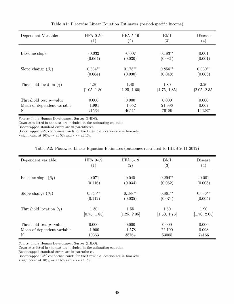
Table A1: Piecewise Linear Equation Estimates (period-specific income)

Dependent Variable: HFA 0-59 HFA 5-19 BMI Disease(1) (2) (3) (4)

Baseline slope -0.032 -0.007 0.183∗∗ 0.001(0.064) (0.030) (0.031) (0.001)

Slope change (β2) 0.334∗∗ 0.178∗∗ 0.856∗∗ 0.030∗∗

(0.064) (0.030) (0.048) (0.003)

Threshold location (γ) 1.30 1.40 1.80 2.20[1.05, 1.80] [1.25, 1.60] [1.75, 1.85] [2.05, 2.35]

Threshold test p−value 0.000 0.000 0.000 0.000Mean of dependent variable -1.991 -1.652 21.996 0.067N 21534 46545 76189 146287

Source: India Human Development Survey (IHDS).Covariates listed in the text are included in the estimating equation.Bootstrapped standard errors are in parentheses.Bootstrapped 95% confidence bands for the threshold location are in brackets.∗ significant at 10%, ∗∗ at 5% and ∗ ∗ ∗ at 1%.

Table A2: Piecewise Linear Equation Estimates (outcomes restricted to IHDS 2011-2012)

Dependent variable: HFA 0-59 HFA 5-19 BMI Disease(1) (2) (3) (4)

Baseline slope (β1) -0.071 0.045 0.294∗∗ -0.001(0.116) (0.034) (0.062) (0.003)

Slope change (β2) 0.345∗∗ 0.188∗∗ 0.861∗∗ 0.036∗∗

(0.112) (0.035) (0.074) (0.005)

Threshold location (γ) 1.30 1.55 1.60 1.90[0.75, 1.85] [1.25, 2.05] [1.50, 1.75] [1.70, 2.05]

Threshold test p−value 0.000 0.000 0.000 0.000Mean of dependent variable -1.900 -1.578 22.190 0.098N 10363 35764 53005 74166

Source: India Human Development Survey (IHDS).Covariates listed in the text are included in the estimating equation.Bootstrapped standard errors are in parentheses.Bootstrapped 95% confidence bands for the threshold location are in brackets.∗ significant at 10%, ∗∗ at 5% and ∗ ∗ ∗ at 1%.

48

Table A3: Piecewise Linear Equation Estimates (household composition included in covariates)

Dependent Variable: HFA 0-59 HFA 5-19 BMI Disease(1) (2) (3) (4)

Baseline slope (β1) -0.022 0.047 0.348∗∗ 0.005∗∗

(0.072) (0.032) (0.046) (0.002)

Slope change (β2) 0.333∗∗ 0.159∗∗ 0.597∗∗ 0.017∗∗

(0.070) (0.032) (0.055) (0.003)

Threshold location (γ) 1.40 1.50 1.70 1.95[1.15, 2.05] [1.20, 1.95] [1.55, 1.85] [1.80, 2.15]

Threshold test p−value 0.000 0.000 0.000 0.000Mean of dependent variable -1.991 -1.649 22.00 0.067N 21634 48845 76949 147729

Source: India Human Development Survey (IHDS).Covariates listed in the text are included in the estimating equation.Bootstrapped standard errors are in parentheses.Bootstrapped 95% confidence bands for the threshold location are in brackets.∗ significant at 10%, ∗∗ at 5% and ∗ ∗ ∗ at 1%.

Table A4: Piecewise Linear Equation Estimates (alternative nutritional status measures)

Dependent variable: WFA 0-59 WFA 5-19 Height(1) (2) (3)

Baseline slope (β1) -0.052 -0.004 0.191(0.055) (0.029) (0.111)

Slope change (β2) 0.287∗∗ 0.331∗∗ 0.836∗∗

(0.055) (0.036) (0.121)

Threshold location (γ) 1.30 1.75 1.45[1.05, 2.20] [1.55, 1.95] [1.30, 1.65]

Threshold test p−value 0.000 0.000 0.000Mean of dependent variable -1.512 -1.635 154.483N 24843 23030 77000

Source: India Human Development Survey (IHDS).Nutritional status for children is measured by weight-for-age (WFA) and for adults by height.Covariates listed in the text are included in the estimating equation.Bootstrapped standard errors are in parentheses.Bootstrapped 95% confidence bands for the threshold location are in brackets.∗ significant at 10%, ∗∗ at 5% and ∗ ∗ ∗ at 1%.

49

Table A5: Piecewise Linear Equation Estimates (IHDS South India)

Dependent variable: HFA 0-59 HFA 5-19 BMI Disease(1) (2) (3) (4)

Baseline slope (β1) 0.014 0.026 0.200∗∗ 0.000(0.065) (0.029) (0.046) (0.003)

Slope change (β2) 0.564∗∗ 0.464∗ 0.961∗∗ 0.025∗∗

(0.065) (0.030) (0.054) (0.005)

Threshold location (γ) 2.60 2.90 1.70 2.00[1.30, 2.00] [2.65, 3.20] [1.55, 1.90] [1.70, 2.30]

Threshold test p−value 0.012 0.000 0.000 0.000Mean of dependent variable -1.792 -1.655 22.186 0.066N 4291 9934 22316 40869

Source: India Human Development Survey (IHDS).Covariates listed in the text are included in the estimating equation.Bootstrapped standard errors are in parentheses.Bootstrapped 95% confidence bands for the threshold location are in brackets.∗ significant at 10%, ∗∗ at 5% and ∗ ∗ ∗ at 1%.

Figure A1: BMI - Income Relationship

(a) Nonparametric relationships BMI - Income

05

10

15

0.5 1.0 1.5 2.0 2.5 3.0

05

10

15

01

23

45

67

F-typestatistic

(present+

mother’sincome)

F-typestatistic

(presentincome)

assumed threshold (log household income)

critical value

full samplereduced sample

(b) Threshold tests

Source: South India Community Health Study (SICHS).Covariates listed in the text are partialled out prior to nonparametric estimation.

50