economic model predictive control of transport-reaction processes
TRANSCRIPT

Economic Model Predictive Control of Transport-ReactionProcesses
Liangfeng Lao, Matthew Ellis and Panagiotis D. Christofides
Department of Chemical & Biomolecular Engineering
Department of Electrical Engineering
University of California, Los Angeles
AIChE Meeting
San Francisco, CA
November 7, 2013
INTRODUCTION
Transport-Reaction Processes
• Examples:
⋄ Fixed bed and tubular reactors
⋄ Fluidized reactors
⋄ Chemical vapor deposition processes
• Process state variables are characterized by strong spatial variations and
nonlinear behavior
⋄ Diffusion and convection phenomena
⋄ Complex reaction mechanisms / Arrhenius dependence of reaction rates on
temperature
• First-principles modeling leads to nonlinear parabolic partial differential equations
(PDEs)

TUBULAR REACTOR EXAMPLE
Concentration Trajectory
• Diffusion-convection-reaction described by a quasi-linear parabolic PDE system:
∂T
∂t= −v
∂T
∂z+
k
ρCp
∂2T
∂z2+
(−∆H
ρCp
)e−E/RTC2
A −hAs
ρCp(T − TC)
∂CA
∂t= −v
∂CA
∂z+DA
∂2CA
∂z2− k0e
−E/RTC2A

BACKGROUND ON CONTROL OF PARABOLIC PDES
• Standard approach: (Ballas, IJC, 1979; Ray, McGraw-Hill, 1981; Curtain, Springer-Verlag, 1978)
⋄ Derivation of ODE models using eigenfunction expansions
⋄ Controller design using methods for ODEs
⋄ High-dimensionality of the controller
• Synthesis of nonlinear low-order controllers: (Christofides, Birkhauser, 2001)
⋄ Derivation of low-order ODE models using Galerkin’s method and
approximate inertial manifolds
⋄ Nonlinear and robust controller synthesis
• Other approaches:
⋄ Passivity-based control approach (Ydstie et al., Syst. & Contr. Lett., 1997)
⋄ Backstepping boundary control (Krstic and Smyshlyaev, SIAM, 2008)
• Model predictive control with quadratic cost functions (Dubljevic et al., Inter. J. Rob. & Non.
Contr., 2006, Comp. & Chem. Eng., 2005)
• Economic model predictive control of transport-reaction processes is an open issue
CONVENTIONAL MPC VS. ECONOMIC MPC
• Conventional MPC
⋄ Quadratic cost function for MPC (Q,R: positive definite matrices)
J =
∫ N∆
0
[(x(τ)− xset)TQ(x(τ)− xset) + (u(τ)− uset)
TR(u(τ)− uset)]dτ
⋄ Penalize the deviation of states and inputs from the steady-state
⋄ Force the system to the economically optimal steady-state
• Lyapunov-based Economic MPC (LEMPC)
⋄ General cost function which accounts for the process economics
J =
∫ N∆
0
L(x(τ), u(τ))dτ
⋄ Use MPC for economic optimization and process control
⋄ Need constraints for closed-loop stability
⋄ Key ideas of our approach:
Utilize Lyapunov-based techniques in the economic MPC formulation
Take advantage of the stability region of an explicit Lyapunov-based controller to
ensure closed-loop stability under LEMPC

LYAPUNOV-BASED ECONOMIC MPC
Two Mode Control Strategy
(M. Heidarinejad, et al., AIChE J. 2012, JPC 2012; S&CL, 2012; 2013)
minimizeu∈S(∆)
∫ tk+N
tk
L(x(τ), u(τ))dτ
subject to ˙x(t) = f(x(t), u(t), 0)
x(tk) = x(tk)
u(t) ∈ U, ∀ t ∈ [tk, tk+N )
V (x(t)) ≤ ρ ∀ t ∈ [tk, tk+N ),
if V (x(tk)) ≤ ρ and tk < t′
∂V
∂xf(x(tk), u(tk), 0)
≤ ∂V
∂xf(x(tk), h(x(tk)), 0)
if V (x(tk)) > ρ and tk ≥ t′
• Economic cost function
• Dynamic model
• Initial condition
• Input constraints
• Mode 1: Boundedness
of closed-loop state
• Mode 2: Convergence
to the origin

LYAPUNOV-BASED ECONOMIC MPC
Two Mode Control Strategy
Ωρ
Ωρ
xs
x(t0)
x(t′)
• Mode 1: Boundedness
of closed-loop state
• Mode 2: Convergence
to the origin

MOTIVATION OF EMPC FOR PDE SYSTEMS
Tubular reactor
• Control objective: maximize the production rate of the product B subject to a
constraint on the available reactant material
⋄ Formulate a model predictive controller that works to directly optimize
objective:
J(x, u) =
∫ tf
0
∫ L
0
k exp
(−E
RT (z, t)
)(CA(z, t))
2 dz dt
⋄ Account for constraint on available reactant material:
1
tf
∫ tf
0
u(τ)dτ = uavailable
• Challanges of applying EMPC to a PDE system
⋄ Construct a finite dimensional model using finite difference method can result
in a high-order model (can be computational inefficient)
⋄ Formulate EMPC with a finite dimensional model of the system

PRESENT WORK
(Lao et al., Ind. & Eng. Chem. Res., 2013; J. Process Contr., submitted)
• Scope:
⋄ Nonlinear parabolic PDEs
⋄ State-feedback Economic Model Predictive Control for PDE systems using
low-order/high-order finite-dimensional models of the PDE system
⋄ Output-feedback Economic Model Predictive Control for PDE systems using
low-order/high-order finite-dimensional models of the PDE system
• Objective:
⋄ Optimally operate a nonlinear parabolic PDE system with EMPC
• Approach:
⋄ Formulate the transport-reaction process as an infinite-dimensional system
⋄ Use Galerkin’s method for modal decomposition of the system
⋄ Take advantage of the stability region of the Lyapunov-based controller
⋄ Perform state-feedback/output-feedback low-order/high-order EMPC design
⋄ Application to a tubular reactor

CLASS OF NONLINEAR PARABOLIC PDE SYSTEMS
• System description
∂x
∂t= A
∂x
∂z+B
∂2x
∂z2+Wu(t) + f(x(z, t))
yj(t) =
∫ 1
0
cj(z)x(z, t)dz, j = 1, · · · , p
⋄ Boundary conditions and initial condition:
∂xj
∂z= g0xj , z = 0;
∂xj
∂z= g1xj , z = 1; x(z, 0) = η(z, 0)
⋄ x ∈ Rn: state vector of the system
⋄ u(t) ∈ Rm: manipulated input vector
⋄ f(x(z, t)) ∈ Rn: nonlinear vector function
⋄ yj(t): the jth measured output
⋄ cj(z): jth sensor distribution function
⋄ z ∈ [0, 1]: the spatial coordinate
⋄ u(t) ∈ U = u ∈ Rm | |ui(t)| ≤ ui,max, i = 1, . . . ,m⋄ A, B, W , g0 and g1: constant matrices and vectors

APPLICATION TO A TUBULAR REACTOR
• A non-isothermal tubular reactor where an irreversible second-order reaction of
the form A → B (exothermic) takes place
• Dynamic model of the process:
∂T
∂t= −v
∂T
∂z+
k
ρCp
∂2T
∂z2+
(−∆H)
ρCpexp
(−E
RT
)CA
2 − hAs
ρCp(T − TC)
∂CA
∂t= −v
∂CA
∂z+DA
∂2CA
∂z2− k0 exp
(−E
RT
)CA
2
• Boundary conditions:
z = 0 :∂T
∂z=
ρCpv
K(T − Tf ),
∂CA
∂z=
v
DA(CA − CAf )
z = L :∂T
∂z= 0,
∂CA
∂z= 0
• Manipulated input: the inlet concentration of species A, CAf

DIMENSIONLESS PDE DYNAMIC MODEL
• Dimensionless form (combining the non-homogeneous part of the boundary
conditions with the differential equation):
∂x1
∂t= −∂x1
∂z+
1
Pe1
∂2x1
∂z2+ βT (Ts − x1) +BTBC exp
(γx1
1 + x1
)(1 + x2)
2
+ δ(z − 0)Ti
∂x2
∂t= −∂x2
∂z+
1
Pe2
∂2x2
∂z2−BC exp
(γx1
1 + x1
)(1 + x2)
2 + δ(z − 0)u
where δ is the standard Dirac function
• Boundary conditions:
z = 0 :∂x1
∂z= Pe1x1,
∂x2
∂z= Pe2x2
z = 1 :∂x1
∂z= 0,
∂x2
∂z= 0
• Process Parameters: Pe1 = 7, P e2 = 7, BT = 2.5, BC = 0.1, βT = 2, Ts = 0, Tf = 0
and γ = 10
GALERKIN’S METHOD
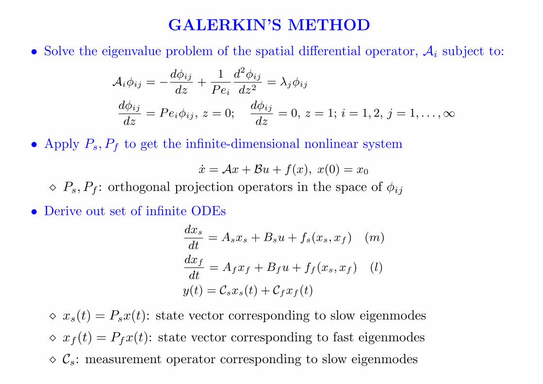
• Solve the eigenvalue problem of the spatial differential operator, Ai subject to:
Aiϕij = −dϕij
dz+
1
Pei
d2ϕij
dz2= λjϕij
dϕij
dz= Peiϕij , z = 0;
dϕij
dz= 0, z = 1; i = 1, 2, j = 1, . . . ,∞
• Apply Ps, Pf to get the infinite-dimensional nonlinear system
x = Ax+ Bu+ f(x), x(0) = x0
⋄ Ps, Pf : orthogonal projection operators in the space of ϕij
• Derive out set of infinite ODEs
dxs
dt= Asxs +Bsu+ fs(xs, xf ) (m)
dxf
dt= Afxf +Bfu+ ff (xs, xf ) (l)
y(t) = Csxs(t) + Cfxf (t)
⋄ xs(t) = Psx(t): state vector corresponding to slow eigenmodes
⋄ xf (t) = Pfx(t): state vector corresponding to fast eigenmodes
⋄ Cs: measurement operator corresponding to slow eigenmodes
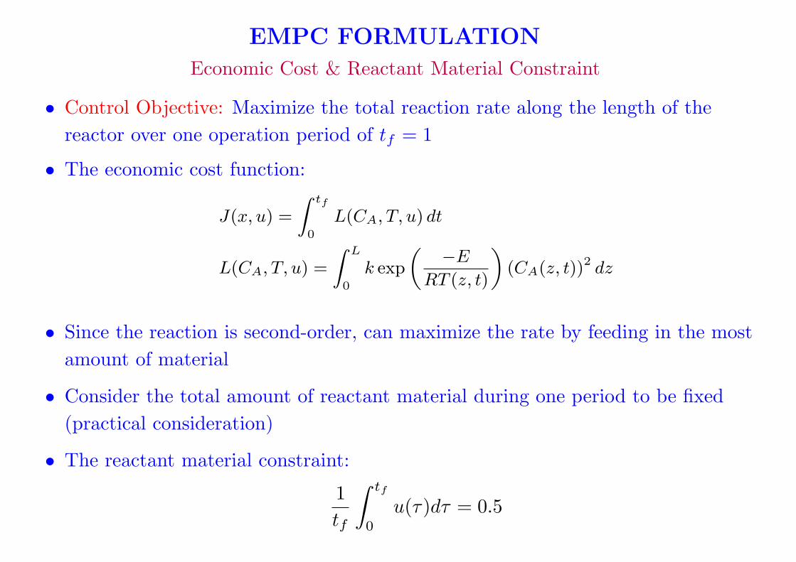
EMPC FORMULATION
Economic Cost & Reactant Material Constraint
• Control Objective: Maximize the total reaction rate along the length of the
reactor over one operation period of tf = 1
• The economic cost function:
J(x, u) =
∫ tf
0
L(CA, T, u) dt
L(CA, T, u) =
∫ L
0
k exp
(−E
RT (z, t)
)(CA(z, t))
2 dz
• Since the reaction is second-order, can maximize the rate by feeding in the most
amount of material
• Consider the total amount of reactant material during one period to be fixed
(practical consideration)
• The reactant material constraint:
1
tf
∫ tf
0
u(τ)dτ = 0.5
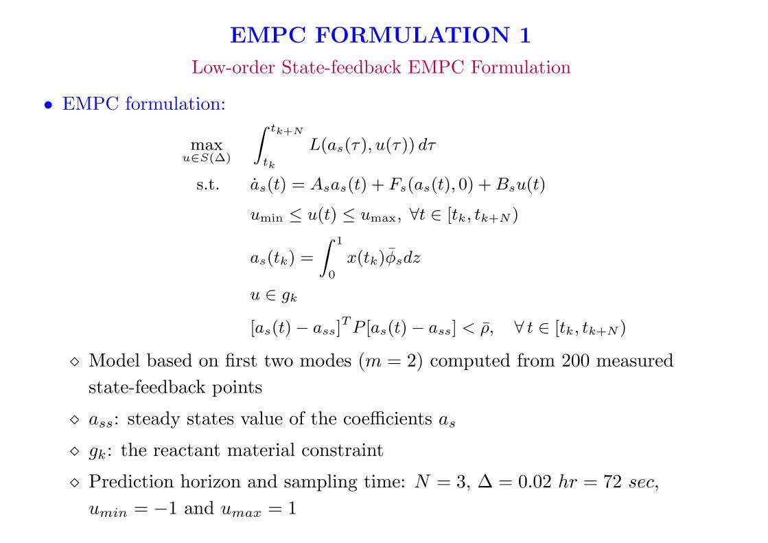
EMPC FORMULATION 1
Low-order State-feedback EMPC Formulation
• EMPC formulation:
maxu∈S(∆)
∫ tk+N
tk
L(as(τ), u(τ)) dτ
s.t. as(t) = Asas(t) + Fs(as(t), 0) +Bsu(t)
umin ≤ u(t) ≤ umax, ∀t ∈ [tk, tk+N )
as(tk) =
∫ 1
0
x(tk)ϕsdz
u ∈ gk
[as(t)− ass]TP [as(t)− ass] < ρ, ∀ t ∈ [tk, tk+N )
⋄ Model based on first two modes (m = 2) computed from 200 measured
state-feedback points
⋄ ass: steady states value of the coefficients as
⋄ gk: the reactant material constraint
⋄ Prediction horizon and sampling time: N = 3, ∆ = 0.02 hr = 72 sec,
umin = −1 and umax = 1
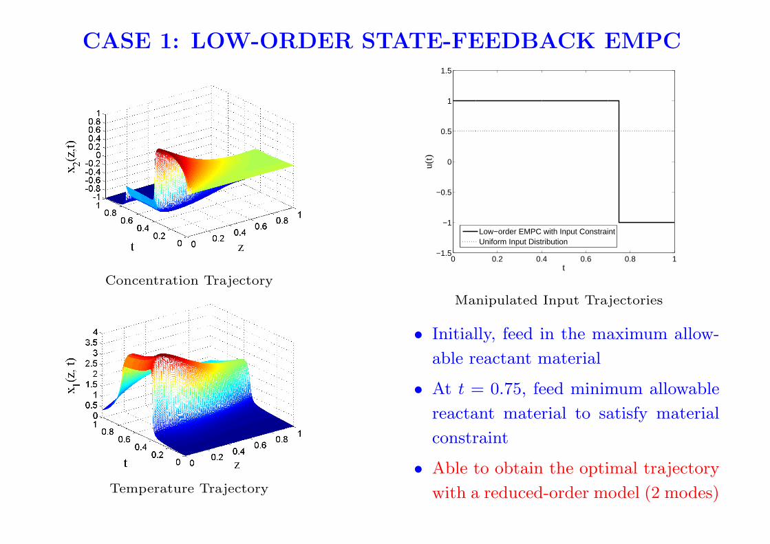
CASE 1: LOW-ORDER STATE-FEEDBACK EMPC
Concentration Trajectory
Temperature Trajectory
0 0.2 0.4 0.6 0.8 1−1.5
−1
−0.5
0
0.5
1
1.5
u(t)
t
Low−order EMPC with Input ConstraintUniform Input Distribution
Manipulated Input Trajectories
• Initially, feed in the maximum allow-
able reactant material
• At t = 0.75, feed minimum allowable
reactant material to satisfy material
constraint
• Able to obtain the optimal trajectory
with a reduced-order model (2 modes)

CASE 1: LOW-ORDER STATE-FEEDBACK EMPC
Comparison with Uniform Material Distribution
Concentration Trajectory
Temperature Trajectory
0 0.2 0.4 0.6 0.8 10
10
20
30
40
50
60
70
t
Rea
ctio
n R
ate,
L(x
,u)
Low−order EMPC with Input ConstraintUniform Input Distribution
Reaction Rate Trajectory
• Average reaction rate from the sys-
tem under EMPC is 9.45% greater
than that from the system under
uniform in time reactant material
distribution
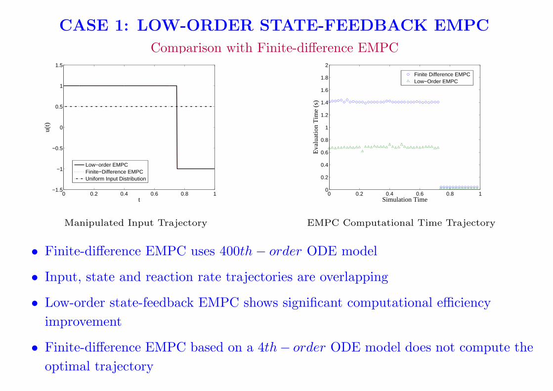
CASE 1: LOW-ORDER STATE-FEEDBACK EMPC
Comparison with Finite-difference EMPC
0 0.2 0.4 0.6 0.8 1−1.5
−1
−0.5
0
0.5
1
1.5
u(t)
t
Low−order EMPCFinite−Difference EMPCUniform Input Distribution
Manipulated Input Trajectory
0 0.2 0.4 0.6 0.8 10
0.2
0.4
0.6
0.8
1
1.2
1.4
1.6
1.8
2
Simulation Time
Eva
luat
ion
Tim
e (s
)
Finite Difference EMPCLow−Order EMPC
EMPC Computational Time Trajectory
• Finite-difference EMPC uses 400th− order ODE model
• Input, state and reaction rate trajectories are overlapping
• Low-order state-feedback EMPC shows significant computational efficiency
improvement
• Finite-difference EMPC based on a 4th− order ODE model does not compute the
optimal trajectory

EMPC FORMULATION 2
High-order State-feedback EMPC Formulation with State and Input Constraints
• Consider a state constraint on the maximum allowable temperature in the reactor
• EMPC formulation:
maxu∈S(∆)
∫ tk+N
tk
L(as(τ), af (τ), u(τ)) dτ
s.t. as(t) = Asas(t) + Fs(as(t), af (t)) +Bsu(t)
af (t) = Afaf (t) +Bfu(t)
umin ≤ u(t) ≤ umax, ∀ t ∈ [tk, tk+N )
amin ≤ a(t) ≤ amax, ∀ t ∈ [tk, tk+N )
as(tk) =
∫ 1
0
x(tk)ϕsdz, af (tk) =
∫ 1
0
x(tk)ϕfdz
a(t) = as(t) + af (t)
u ∈ gk
[a(t)− ass]TP [a(t)− ass] < ρ, ∀ t ∈ [tk, tk+N )
⋄ Slow subsystem based on the first 10 modes
⋄ Fast subsystem based on the next 190 modes
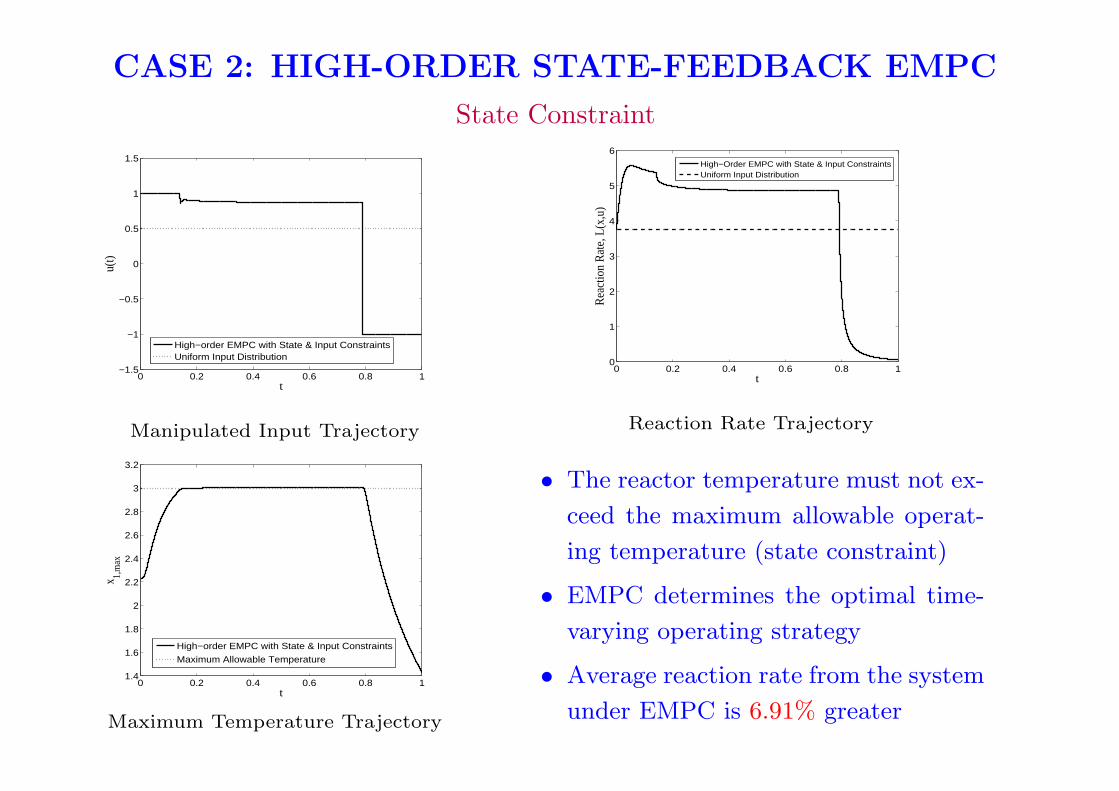
CASE 2: HIGH-ORDER STATE-FEEDBACK EMPC
State Constraint
0 0.2 0.4 0.6 0.8 1−1.5
−1
−0.5
0
0.5
1
1.5
u(t)
t
High−order EMPC with State & Input ConstraintsUniform Input Distribution
Manipulated Input Trajectory
0 0.2 0.4 0.6 0.8 11.4
1.6
1.8
2
2.2
2.4
2.6
2.8
3
3.2
x 1,m
ax
t
High−order EMPC with State & Input Constraints
Maximum Allowable Temperature
Maximum Temperature Trajectory
0 0.2 0.4 0.6 0.8 10
1
2
3
4
5
6
t
Rea
ctio
n R
ate,
L(x
,u)
High−Order EMPC with State & Input ConstraintsUniform Input Distribution
Reaction Rate Trajectory
• The reactor temperature must not ex-
ceed the maximum allowable operat-
ing temperature (state constraint)
• EMPC determines the optimal time-
varying operating strategy
• Average reaction rate from the system
under EMPC is 6.91% greater
EMPC FORMULATION 3
State Estimation Using Output Feedback Methodology
• State Estimation: Use a finite number, p, of measured outputs yj(t) (here, we
choose state-feedback measured points) (j = 1, · · · , p) to compute estimates of asand af with the assumption:
p = m
C−1s exists
• The estimates of the slow modes, as(t) is obtained from a direct inversion of the
measured output map:
as(t) = C−1s y(t)
• The fast dynamics af (t) can be ignored (given that Af includes eigenvalues with
large negative real part) compared with the slow dynamics as(t)
• An explicit form for the estimated fast modes, af :
af (t) = −A−1f [Bfu(t) + ff (as(t), 0)]
EMPC FORMULATION 3
Low-order Output-feedback EMPC
• EMPC formulation:
maxu∈S(∆)
∫ ttk+N
tk
L(as(τ), u(τ))dτ
s.t. ˙as(t) = Asas(t) + Fs(as(t), 0) + Bsu(t)
as(tk) = C−1s y(tk)
umin ≤ u(t) ≤ umax
u ∈ gk
as,min ≤ as(t) ≤ as,max
[as(t)− ass]TP [as(t)− ass] < ρ, ∀ t ∈ [tk, tk+N )
⋄ Model based on first 11/21 modes (m = 11/21) computed from 11 measured
state-feedback points (p = 11/21)
⋄ as(t): predicted slow mode function of as(t)
⋄ Prediction horizon and sampling time: N = 3, ∆ = 0.01 hr = 36 sec,
umin = −1 and umax = 1

CASE 3: LOW-ORDER OUTPUT-FEEDBACK EMPC
Maximum Temperature and Manipulated Input Trajectories
0 0.1 0.2 0.3 0.4 0.5 0.6 0.7 0.8 0.9 1−1.5
−1
−0.5
0
0.5
1
1.5
t
u(t)
11 Slow Modes21 Slow ModesUniform Input, u(t) = 0.5
Manipulated Input Trajectory
0 0.1 0.2 0.3 0.4 0.5 0.6 0.7 0.8 0.9 11.4
1.6
1.8
2
2.2
2.4
2.6
2.8
3
3.2
t
x 1,m
ax
21 Slow Modes11 Slow ModesMaximum Allowable Temperature
Maximum Temperature Trajectory
0 0.1 0.2 0.3 0.4 0.5 0.6 0.7 0.8 0.9 10
1
2
3
4
5
6
t
Rea
ctio
n R
ate,
L(x
,u)
11 Slow Modes21 Slow ModesUniform Input, u(t) = 0.5
Reaction Rate Trajectory
• EMPC based on 21 slow modes computes
a smoother manipulated input profile
• Average reaction rate from the EMPC
based on 21 slow modes is 5.13% greater
than that of EMPC based on 11 slow
modes and 8.45% greater than that of the
system with uniform in time reactant ma-
terial distribution

EMPC FORMULATION 4High-order Output-feedback EMPC Formulation
• EMPC formulation:
maxu∈S(∆)
∫ ttk+N
tk
L(as(τ), af (τ), u(τ))dτ
s.t. ˙as(t) = Asas(t) + Fs(as(t), af (t)) + Bsu(t)
as(tk) = C−1s y(tk)
af (t) = −A−1f [Bfu(t) + ff (as(t), 0)]
a(t) = as(t) + af (t)
umin ≤ u(t) ≤ umax
u ∈ gk
amin ≤ a(t) ≤ amax
[a(t)− as]TP [a(t)− as] < ρ, ∀ t ∈ [tk, tk+N )
⋄ Model based on first 30 modes which include 11 slow modes and 19 fast modes
(m = 11, l = 19) computed from 11 measured state-feedback points (p = 11)
⋄ af (t): predicted fast mode function of af (t)
⋄ a(t): predicted finite mode function of a(t)
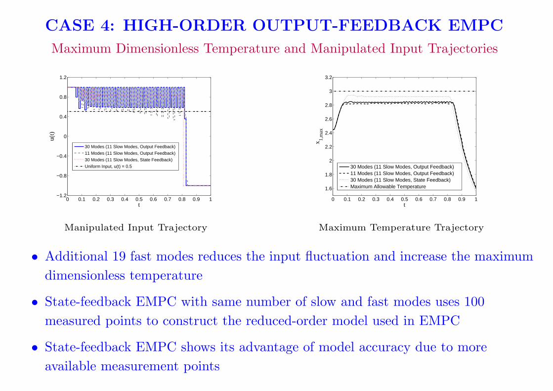
CASE 4: HIGH-ORDER OUTPUT-FEEDBACK EMPC
Maximum Dimensionless Temperature and Manipulated Input Trajectories
0 0.1 0.2 0.3 0.4 0.5 0.6 0.7 0.8 0.9 1−1.2
−0.8
−0.4
0
0.4
0.8
1.2
t
u(t)
30 Modes (11 Slow Modes, Output Feedback)
11 Modes (11 Slow Modes, Output Feedback)
30 Modes (11 Slow Modes, State Feedback)
Uniform Input, u(t) = 0.5
Manipulated Input Trajectory
0 0.1 0.2 0.3 0.4 0.5 0.6 0.7 0.8 0.9 1
1.6
1.8
2
2.2
2.4
2.6
2.8
3
3.2
t
x 1,m
ax
30 Modes (11 Slow Modes, Output Feedback)11 Modes (11 Slow Modes, Output Feedback)30 Modes (11 Slow Modes, State Feedback)Maximum Allowable Temperature
Maximum Temperature Trajectory
• Additional 19 fast modes reduces the input fluctuation and increase the maximum
dimensionless temperature
• State-feedback EMPC with same number of slow and fast modes uses 100
measured points to construct the reduced-order model used in EMPC
• State-feedback EMPC shows its advantage of model accuracy due to more
available measurement points

CASE 4: HIGH-ORDER OUTPUT-FEEDBACK EMPC
Reaction Rate and Computational Time Trajectories
0 0.1 0.2 0.3 0.4 0.5 0.6 0.7 0.8 0.9 10
1
2
3
4
5
6
t
Rea
ctio
n R
ate,
L(x
,u)
30 Modes (11 Slow Modes, Output Feedback)
11 Modes (11 Slow Modes, Output Feedback)
30 Modes (11 Slow Modes, State Feedback)
Uniform Input, u(t) = 0.5
Reaction Rate Trajectory
0 0.1 0.2 0.3 0.4 0.5 0.6 0.7 0.8 0.9 10
10
20
30
40
50
60
70
t
Com
puta
tiona
l Tim
e Pr
ofile
/ se
c
30 Modes (11 Slow Modes, Output Feedback)11 Modes (11 Slow Modes, Output Feedback)30 Modes (11 Slow Modes, State Feedback)
EMPC Computational Time Trajectory
• Average reaction rate from the high-order output feedback EMPC is 0.89%
greater than that from the low-order output feedback EMPC system
• Average reaction rate from the high-order output feedback EMPC system is
0.73% less than that from the EMPC system with state feedback
• The average computational efficiency of the high-order output feedback EMPC
system is comparable to that of the state feedback EMPC system

CONCLUSIONS
• Proposed EMPC formulation for nonlinear parabolic PDE systems
⋄ Use Galerkin’s method to realize order reduction of nonlinear parabolic PDE
model
⋄ Perform low/high-order state/output-feedback EMPC formulations
• Application to a tubular reactor
⋄ Demonstrated the ability to maximize the economic cost by following a
time-varying input trajectory
⋄ Demonstrated the ability to satisfy a state constraint on the maximum
allowable temperature
⋄ Compared the output-feedback and state-feedback EMPC performance on
model accuracy, objective optimization and computational efficiency
ACKNOWLEDGEMENT
Financial support from the National Science Foundation and Department of Energy is
gratefully acknowledged