economic models for social interactions · economic models for social interactions larry blume...
TRANSCRIPT

Economic Models for Social Interactions
Larry Blume
Cornell University & IHS & The Santa Fe Institute & HCEO
SSSI 2016Chicago

Introduction
2 / 150

Social Life and Economics
I “The outstanding discovery of recent historical andanthropological research is that man’s economy, as a rule, issubmerged in his social relationships. He does not act so asto safeguard his individual interest in the possession ofmaterial goods; he acts so as to safeguard his social standing,his social claims, his social assets. He values material goodsonly in so far as they serve this end.” (Polanyi, 1944)
I “Economics is all about how people make choices. Sociologyis all about why they don’t have any choices to make.”(Duesenberry, 1960)
3 / 150

Where do Social Interactions Appear?
Phenomena
I Labor marketsI Career ChoicesI Retirement
I Fertility
I Health
I Education Outcomes
I Violence
Mechanisms
I Peer effectsI Stigma
I Role models
I Social Norms
I Social Learning
I Social Capital?
4 / 150

Questions
I What are appropriate tools for modelling social interactions?
I Models of social interactions: Social norms, groupmembership, peer effects.
I Describe the peer effects. What goes on at the micro level?
I What are the aggregate effects of interaction on socialnetworks?
5 / 150

Plan
I Network Science
I Labor Markets — Weak and Strong Ties
I Peer Effects and Complementarities — Games on Networks
I Matching and Network Formation
I Social Capital
I Social Learning
I Diffusion
6 / 150

Network Science
7 / 150

GraphsA directed graph G is a pair (V ,E) where V is a set of vertices, ornodes, and E is a set of Edges. In a directed graph, an edge is anordered pair (v,w) of vertices, meaning that there is a connectionfrom v to w. In an undirected graph, an edge is an unordered pairof vertices.
A B
C
D
V =A ,B,C,D
G =
(A ,B), (B,C), (B,D)
A B
C
D
V =A ,B,C,D
G =
(A ,B), (C,B),
(B,D), (D,B)
8 / 150

The degree of a node in an undirected graph G is#w : (v,w) ∈ E.
A path of G is an ordered list of nodes (v0, . . . , vN) such that(vn−1, vn) ∈ E for all 1 ≤ n ≤ N. A geodesic is a shortest-lengthpath connecting v0 and vn.
A B
C
D
degC = 1.
A B
C
D
(C,B,D)
9 / 150

Graphs
A subset of vertices is connected if there is a path between everytwo of them. A component of G is a set of vertices maximal withrespect to connectedness. A clique is a component for which allpossible edges are in E.
10 / 150

A graph G has a matrix representation. A adjacency matrix for agraph (V ,E) is a #V ×#V matrix A such that avw = 1 if(v,w) ∈ E, and 0 otherwise. A weighted adjacency matrix hasnon-zero numbers corresponding to edges in E.
0 1 1 0 0 0 0 01 0 0 1 0 0 0 01 0 0 1 0 0 0 00 1 1 0 0 0 0 00 0 0 0 0 1 1 10 0 0 0 1 0 1 10 0 0 0 1 1 0 10 0 0 0 1 1 1 0
11 / 150

Graphs
I 3 Components,A ,B, C,D,E,F , . . . ,M.
I Min degree = 1.I Max deg = 4.I Diam Comp. 3 = 3.I Degree Dist. 1 :
4/13, 2 : 4/13, 3 :4/13, 4 : 1/13.
12 / 150

Common Network Measurements
I Graph diameter — maximal geodesic length.
I Mean geodesic length.
I Degree distribution.
I Clustering coefficient — the average (over vertices) of thenumber of length 2 paths containing i that are part of atriangle. (Measures degree of transitivity.)
I Component size distribution
13 / 150

Some Social Networks
n – # nodes, m – # edges, z – mean degree,l – mean geodesic length, α – exponent of degree dist.,
C(k ) - clustering coeff.s, r degree corr. coeff.
14 / 150

Crime Micro Analysis
Mennis and Harris (2001)
Although other research has investigated deviant peercontagion, and still other research has examined offensespecialization among delinquent youths, we have foundthat deviant peer contagion influences juvenile recidi-vism, and that contagion is likely to be associated withrepeat offending. These findings suggest that juvenilesare drawn to specific types of offending by the spatially-bounded concentration of repeat offending among theirpeers. Research on causes of delinquency within neigh-borhoods, then, may produce more useful causal modelsthan studies that ignore spatial concentrations of offensepatterns.
15 / 150

Crime Micro Analysis
16 / 150

Crime Micro Analysis
17 / 150

Aggregate Analysis
Glaeser Sacerdote and Scheinkman (1996). “Crime and SocialInteraction.”
The most puzzling aspect of crime is not its overall levelnor the relationships between it and either deterrence oreconomic opportunity. Rather, following Quetelet [1835],we believe that the most intriguing aspect of crime is itsastoundingly high variance across time and space.
Positive covariance across agents’ decisions about crimeis the only explanation for variance in crime rates higherthan the variance predicted by difference in localconditions.
18 / 150
A Model (of sorts)
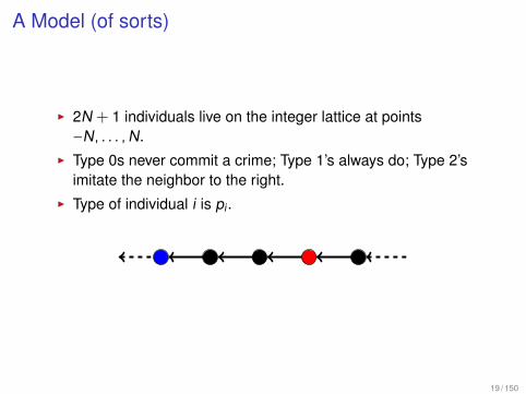
I 2N + 1 individuals live on the integer lattice at points−N, . . . ,N.
I Type 0s never commit a crime; Type 1’s always do; Type 2’simitate the neighbor to the right.
I Type of individual i is pi .
19 / 150

A Model (of sorts)
I Expected distance between fixed agents determines groupsize — range of interaction effects.
I Social interactions magnify the effect of fixed agents.
Eai =p1
p0 + p1≡ p, Sn =
∑|i|≤n
ai − p2n + 1
.
√2n + 1Sn → N(0,σ2), σ2 = p(1 − p)
2 − ππ
where
π = p0 + p1, f(π) =2 − ππ
.
20 / 150

Aggregate Statistics
21 / 150
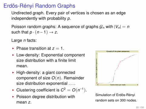
Erdös-Rényi Random GraphsUndirected graph. Every pair of vertices is chosen as an edgeindependently with probability p.
Poisson random graphs: A sequence of graphs Gn with |Vn | = nsuch that p · (n − 1)→ z.
Large n facts:
I Phase transition at z = 1.I Low-density: Exponential component
size distribution with a finite limitmean.
I High-density: a giant connectedcomponent of size O(n). Remaindersize distribution exponential . . . .
I Clustering coefficient is C2 = O(n−1).I Poisson degree distribution with
mean z.
Simulation of Erdös-Rényi
random sets on 300 nodes.
22 / 150

Preferential Attachment
I A source of power laws.
I Introduced by Eggenberger and Polya (1923).
I Popularized by Zipf (1949) (city size) and Simon (1955)(wealth).
23 / 150

Preferential Attachment
A directed graph.I A vertex set V of size N.I For nodes i > 1, with probability p i links to a randomly chosen
node j < i.I With probability (1 − p) i links to the immediate ancestor of j.
The graph is surely connected.
For large n the fraction of nodes with in-degree k is 1/k r where rdepends on p. The fraction Pr of vertices with r edges converges
as N gets large, and Pr = Θ(r−2−p1−p ). See Kumar et al. (2000).
24 / 150

Preferential Attachment
25 / 150

Some Social Networks I
26 / 150

Some Social Networks II
27 / 150

Some Social Networks III
28 / 150

Transitivity
“If two people in a social network have a friend in common, thenthere is an increased likelihood that they will become friendsthemselves at some point in the future.” Rappoport (1953)
I Clustering coefficient:Fraction of connected triplesthat are triangles.
I Why transitivity?A
B
C
29 / 150

Centrality
Types of Centrality Measures:
Degree Centrality How many vertices can a vertex reach directly?
Betweeness Centrality How likely is this vertex to be on thegeodesic between two randomly chosen vertices?
Closeness Centrality How fast can this vertex reach all vertices inthe network.
Eigenvector Centrality How much does this vertex influence otherimportant vertices?
30 / 150

Centrality Degree Centrality
Which nodes are important?
Let A be the adjacency matrix for a directed graph. Aij = 1 if jinfluences i. e is the vector of 1’s.
I Degree Centraility: How many nodes can a node directlyinfluence?
‘
cd = eA cj =∑
i
Aij
31 / 150

Centrality Katz Centrality
I Katz (1953) Centrality: How many nodes can a node reach?
ckj (α) =
∑i
∑k>0
αk Ak
ij
c(α) = (I − αA)−1e − e.
Akij is the number of paths of length k from i to j. The parameter α
discounts longer paths. α must be less than the largest eigenvalueof A .
32 / 150

Centrality Eigenvector Centrality
I Eigenvector Centrality: The centrality of j is proportional to thesum of the centralities of the nodes she influences.
cej = µ
∑i
ciaij
where µ > 0. If the network is strongly connected, then(Perron Frobenius Theorem) there is a unique scalar µ and aone-dimensional set of vectors c 0 that solve this. µ is theinverse of the Perron eigenvalue, and c is in the correspondingleft eigenspace. (Bonacich, 1987; Bonacich and Lloyd, 2001).
33 / 150

Centrality Eigenvector Centrality
Suppose A is indecomposable and aperiodic. Let λ ≥ 1 denote thePerron eigenvalue of A . Then B = λ−1A has Perron eigenvalue 1.Let v denote a (strictly positive) Perron right eigenvector of A , andV the diagonal matrix whose ith diagonal element is vi . ThenM = V−1BV is a Markov matrix, with a unique invariant vector ofl1-norm 1. Let π be that vector.
π = πM
= πV−1BV
πV−1 = πV−1B
so πV−1 is left-invariant under A and thus a centrality vector.
34 / 150

Centrality Eigenvector Centrality
Ck (α) is the diagonal matrix with diagonal elements cki (α),
α < 1/λ.
I + Ck (β/λ) =∑k≥0
βkλ−k Ak =∑k≥0
βk Bk
=∑k≥0
βk (VMV−1)k = V
∑k≥0
βk Mk
V−1
(1 − β)I + (1 − β)V−1Ck (β/λ)V = (1 − β)∑k≥0
βk Mk β→1−−−→ Π
limβ→1
(1 − β)Ck (β/λ) = VCe
as β→ 1, that is, α→ 1/λ.
To round this out, limα→0 α−1ck (α) = cd .
35 / 150

Centrality α-Centrality
Two sources of centrality:I Who you are connected to.I What you ‘bring to the table’.
cα(d) = αcαA + d
= d(I − αA)−1
= d(I + αA + α2A2 + · · · )
α-centrality takes d = e:
cα = cα(e).
36 / 150

Centrality α-CentralityA quadratic game in which each player is influenced by theaverage play of his neighbors.
ui(xi, x−i) = hixi −x2
i
2−β
2(xi − xi)
2, xi =∑
j
aijxj.
The equilibrium is unique:
x = (1 − φ)(I − φA)−1h, φ = β/1 + β.
Average play in the population is
1n
e · x =1 − φ
ne (I − φA)−1 h
=1n(1 − φ)cφh.
Individual i’s influence on the average choice of the population isproportional to cφ.
37 / 150

Homophily
“Similarity begets friendships.”Plato
“All things akin and like are forthe most part pleasant to eachother, as man to man, horse tohorse, youth to youth. This is theorigin of the proverbs: The oldhave charms for the old, theyoung for the young, like to like,beast knows beast, ever jackdawto jackdaw, and all similarsayings.” Aristotle,Nicomachean Ethics
38 / 150
Sources of Homophily
I Status Homophily: We feel more comfortable when weinteract with others who share a similar cultural background.
I Value Homophily: We often feel justified in our opinions whenwe are surrounded by others who share the same beliefs.
I Opportunity Homophily: We mostly meet people like us.
39 / 150

Sources of Homophily
I Fixed attributesI Selection
I Variable attributesI Social influence
I Identification
40 / 150

Measuring Homophily
Consider a network with N individuals: Fraction p are males,fraction q = 1 − p are females.
I Assign nodes to gender randomly, each node male withprobability p.
I What is the probability of a “cross-gender” edge?
I A fraction of cross-gender edges less than 2pq is evidence forhomophily.
41 / 150

Labor Markets

Inequality in Labor Markets
43 / 150

Inequality in Labor Markets
44 / 150

Job Search
45 / 150

The Strentgh of Weak Ties
“. . . [T]he strength of a tie is a (probably linear) combination of theamount of time, the emotional intensity, the intimacy (mutualconfiding), and the reciprocal services which characterize the tie.Each of these is somewhat independent of the other, though theset is obviously highly intracorrelated. Discussion of operationalmeasures of and weights attaching to each of the four elements ispostponed to future empirical studies. It is sufficient for the presentpurpose if most of us can agree, on a rough intuitive basis,whether a given tie is strong, weak, or absent.”
Granovetter (1973, p. 1361)
46 / 150

Why do Weak Ties Matter? I
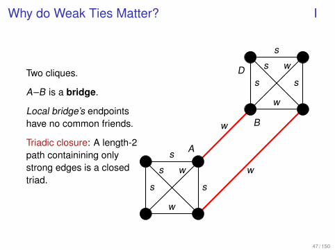
Two cliques.
A–B is a bridge.
Local bridge’s endpointshave no common friends.
Triadic closure: A length-2path containining onlystrong edges is a closedtriad.
A
B
47 / 150

Why do Weak Ties Matter? I
Two cliques.
A–B is a bridge.
Local bridge’s endpointshave no common friends.
Triadic closure: A length-2path containining onlystrong edges is a closedtriad.
A
B
47 / 150

Why do Weak Ties Matter? I
Two cliques.
A–B is a bridge.
Local bridge’s endpointshave no common friends.
Triadic closure: A length-2path containining onlystrong edges is a closedtriad.
A
B
47 / 150
Why do Weak Ties Matter? I
Two cliques.
A–B is a bridge.
Local bridge’s endpointshave no common friends.
Triadic closure: A length-2path containining onlystrong edges is a closedtriad.
A
B
s
w
s s
ws
s
w
s s
ws
w
w
D
47 / 150

Ties and Inequality IMontgomery (1991)
I Workers live for two periods, #W identical in both periods.I Half of the workers are high-ability, produce 1.I Half of the workers are low-ability, produce 0.I Workers are observationally indistinguishable.
I Each firm employs 1 worker.I π = employee productivity −wage.I Free entry, risk-neutral entrepreneurs.
I Equilibrium condition: Firms expected profit is 0. Wage offersare expected productivity.
48 / 150

Ties and Inequality IISocial Structure
I Each t = 1 worker knows at most 1 t = 2 worker.I Each t = 1 worker has a social tie with pr = τ.I Conditional on having a tie, it is to the same type with
probability α > 1/2.I Assignments of a t = 1 worker to a specific t = 2 worker is
random.
I τ — “network density”I α — “inbreeding bias”
49 / 150

Ties and Inequality IIITiming
I Firms hire period 1 workersthrough the anonymousmarket, clears at wage wm1.
I Production occures. Eachfirm learns its worker’sproductivity.
I Firm f sets a referral offer,wrf , for a second periodworker.
I Social ties are assigned.
I t = 1 workers with ties relaywri .
I t = 2 workers decide eitherto accept an offer or enterthe market.
I Period 2 market clears atwage wm2.
I Production occurs
50 / 150

Ties and Inequality IVEquilibrium
I Only firms with 1-workers will make referral offers.
I Referral wages offers are distributed on an interval [wm2,wR ].
I 0 < wm2 < 1/2.
I π2 > 0.
I wm1 = E
production value + referral value> 1/2.
51 / 150

Ties and Inequality VComparative Statics
α, τ ↑ =⇒
wm2 ↓
wR ↑
π2 ↑
wm1 ↑
52 / 150

Ties and Inequality VIComparing Models
I in the market-only model, wm1 = wm2 = 1/2.
I t = 2 1-types are better off, t = 2 low types are worse off.Social structure magnifies income inequality in the secondperiod.
I The total wage bill in the second period is less with socialstructure.
53 / 150

Weak Ties in China
Tian, Felicia and Nan Lin. 2016. “Weak ties, strong ties, and jobmobility in urban China: 1978–2008”. Social Networks 44,117–129.
. . . Using pooled data from three cross-sectional surveys in urbanChina, the results show a steady increase in the use of weak tiesand an increasing and persistent use of strong ties in finding jobsbetween 1978 and 2008. The results also show no systematicdifference between the use of weak ties for finding jobs in themarket sector versus the state sector. However, they show fastergrowth in the use of strong ties for finding jobs in the state sector,compared to the market sector.
54 / 150

Peer Effectsand Complementarities
Behaviors on Networks
55 / 150

Three Types of Network Effects
I Information and social learning.
I Network externalities.
I Social norms.
56 / 150

A Common Regression
ωi = π0 + xiπ1 + xgπ2 + ygπ3 + εi
WhereI ωi is a choice variable for an individual,I xi is a vector of individual correlates,I xg is a vector of group averages of individual correlates,I yg is a vector of other group effects, andI εi is an unobserved individual effect.
57 / 150

LIM Model The Reflection Problem
For all g ∈ G and all i ∈ g,
ωi = α+ βxi + δxg + γµi + εi (Behavior)
xg =1
Ngxi (Behavior)
µi =1
Ng
∑j∈g
Eωj
(Equilibrium)
The reduced form is
ωi =α
1 − γ+ βxi +
γβ+ δ
1 − γxg + εi
58 / 150

General Linear Network Model
ωi = β′xi + δ′∑
j
cijxj + γ′∑
j
aij Eωj |x
+ ηi
This is the general linear model
Γω+ ∆x = η.
Question:I How do we interpret the parameters?I What kind of restrictions on the coefficients are reasonable,
and do they lead to identification.
These questions require a theoretical foundation.
59 / 150

Incomplete-Information Game
I I individuals; each i described by a type vector (xi, zi) ∈ R2.xi is publicly observable, zi is private.
I There is a Harsanyi prior ρ on the space of types R2I.I Actions are ωi ∈ R.I Payoff functions:
Ui(ωi,ω−i; x, zi) = θiωi −12ω2
i −φ
2
ωi −∑
j
aij ωj
2
I aij — peer effect of j on i.
60 / 150

Private Component
To complete the model, specify how individual characteristicsmatter.
θi = γxi + δ∑
j
cijxj + z
Direct Effect Contextual Effect
cij — contextual/direct effect of j on i.
61 / 150

Equilibrium
(1 + φ)
(I −
φ
1 + φA)ω − (γI + δC)x = η
Γω+ ∆x = η.
Constraints imposed by the theory:
aii = cii = 0,∑
j
aij =∑
j
cij = 1.
Γii = 1 + φ,∑j,i
Γij = −φ, ∆ii = −(γ+ δ),∑j,i
∆ij = δ.
Even more constraints if you insist on A = C.
62 / 150
Classical Econometrics Rank and Order Conditions
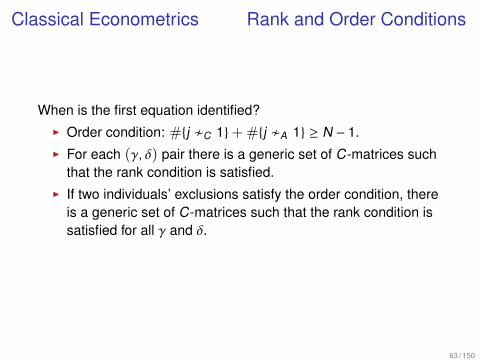
When is the first equation identified?I Order condition: #j /C 1+#j /A 1 ≥ N − 1.I For each (γ, δ) pair there is a generic set of C-matrices such
that the rank condition is satisfied.I If two individuals’ exclusions satisfy the order condition, there
is a generic set of C-matrices such that the rank condition issatisfied for all γ and δ.
63 / 150

Non-Linear Aggregators
Bad apple The worst student does enormous harm.
Shining light A single student with sterling outcomes can inspireall others to raise their achievement.
Invidious comparison Outcomes are harmed by the presence ofbetter achieving peers.
Boutique A student will have higher achievement whenever sheis surrounded by peer with similar characteristics.
64 / 150

Matching and NetworkFormation
65 / 150

I Market Design
I Matching problems are models of network formation
I Bipartite matching with transferable utilityI Bipartite matching without exchangeI Generalization to networks
66 / 150

Stable Matches
Given are two sets of objects X and Y . e.g. workers and firms.Both sides have preferences over whom they are matched with,but with no externalities, that is, given that a is matched with x, hedoes not care if b is matched with y and z. The literature dividesover the information parties have when they choose partners, andwhether compensating transfers can be made. The organizingprinciple is that of a stable match.
Assume w.l.o.g. |X | ≤ |Y |.
Definition: A match is one-to-one map from X to Y . A match isstable if there are no pairs x ↔ y and x′ ↔ y′ such that y′ x yand x y′ x′.
67 / 150

Transferable Utility Optimality
Find the optimal match by maximizing total surplus:
v(L ∪ F) = maxx
∑l,f
vlf xlf
s.t.∑
f
xlf ≤ 1 for all l,∑l
xlf ≤ 1 for all f ,
x ≥ 0
The vertices for this problem are integer solutions, that is,non-fractional matches. A solution to the primal is an optimalmatching.
68 / 150

Transferable Utility Stability
Set of laborers L and firms F . vlf is the value or surplus generatedby matching worker l and firm f .
The surplus of a match is split between the firm and worker.Suppose i ↔ f and j ↔ g. Payments to each are wi and wj , and πi
and πj .
Since this is a division of the surplus,
wi + πf = vif and wj + πg = vjg.
If wi + πg < vig, then there is a split of the surplus vig such that iand g would both prefer to match with each other than with theircurrent partners. The match is not stable. Stability requires
wi + πg ≥ vig and wj + πf ≥ vjf .
69 / 150

Matching with Transferable Utility
The dual has variables for each individual and firm.
minw,π
∑l,f
wl + πf
s.t. πf + wl ≥ vlf for all pairs l, f ,
π ≥ 0, w ≥ 0.
Solutions to the dual satisfy the stability condition.
Complementary slackness says that matched laborer-firm pairssplit the surplus, πf + wl = vlf .
70 / 150

Characterizing Matches
Theorem: A matching is stable if and onl if it is optimal.
Lemma: Each laborer with a positive payoff in any stable outcomeis matched in every stable matching.
Proof: Complementary slackness.
Lemma: If laborer l is matched to firm f at stable matching x, andthere is another stable matching x′ which l likes more, then f likesit less.
Proof: Formalize this as follows: If x is a stable matching and〈w′, π′〉 is another stable payoff, then w′ > w implies π > π′. Thisfollows from complementary slackness, sincewl + πf = vlf = w′l + π′f .
71 / 150

Assortative Matching ComplementaritiesSuppose X and Y are each partially-ordered sets, andv : X × Y → R is a function.
Definition: v : X × Y → R has increasing differences iff x′ > x andy′ > y implies that
v(x′, y′) + v(x, y) ≥ v(x′, y) + v(x, y′).
An important special case is where X and Y are intervals of R,each with the usual order, and v is C2.
v(x′, y′) − v(x, y′) ≥ v(x′, y) − v(x, y).
Then
Dxv(x, y′) ≥ Dxv(x, y)
From this it follows that Dxyv(x, y) ≥ 0.
72 / 150

Generalizations
I Matching without exchange. Gale and Shapley (1962).
I The roommate problem.
I Generalization of non-transferable matching to networks.Jackson and Wolinsky (1996).
73 / 150
Network Formation with Contagious Risk
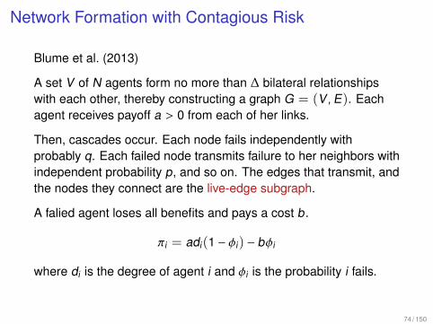
Blume et al. (2013)
A set V of N agents form no more than ∆ bilateral relationshipswith each other, thereby constructing a graph G = (V ,E). Eachagent receives payoff a > 0 from each of her links.
Then, cascades occur. Each node fails independently withprobably q. Each failed node transmits failure to her neighbors withindependent probability p, and so on. The edges that transmit, andthe nodes they connect are the live-edge subgraph.
A falied agent loses all benefits and pays a cost b.
πi = adi(1 − φi) − bφi
where di is the degree of agent i and φi is the probability i fails.
74 / 150

Network Formation with Contagious Risk
Rawlsian welfare — minimum welfare among all agents.
Definition: A graph is stable if:I no node can strictly increase its payoff by deleting all its
incident links (hence removing itself from the network), andI there is no pair of unconnected nodes (i, j) such that adding
an (i, j) edge to G would make them both better off.
75 / 150

Assumptions
I a > pqb.I a < pb.I a < qb.
We want the bounds to hold very loosely. “Separation parameter”δ:
Assumption P(δ): There is a small constant δ such that
δ−1pqb < a < δminpb, qb.
76 / 150

I Results provide asymptotically tight characterizations of thewelfare obtained by both socially optimal and stable graphs.
I If each node forms more than 1/p links, the live-edgesubgraph has a giant connected component.
I “. . . , we find roughly that social optimality occurs just beyondthe edge of a phase transition that controls how failurespropagate, while stable graphs lie slightly further still past thisphase transition, at a point where most of the welfare hasalready been wiped out.”
77 / 150

Social Capital
78 / 150

Networks and Social Capital
“the aggregate of the actual or potential resources which are linked to possessionof a durable network of more or less institutionalized relationships of mutualacquaintance or recognition.” (Bourdieux and Wacquant, 1992)
“the ability of actors to secure benefits by virtue of membership in social networksor other social structures.” (Portes, 1998)
“features of social organization such as networks, norms, and social trust thatfacilitate coordination and cooperation for mutual benefit.” (Putnam, 1995)
“Social capital is a capability that arises from the prevalence of trust in a societyor in certain parts of it. It can be embodied in the smallest and most basic socialgroup, the family, as well as the largest of all groups, the nation, and in all theother groups in between. Social capital differs from other forms of human capitalinsofar as it is usually created and transmitted through cultural mechanisms likereligion, tradition, or historical habit.” (Fukuyama, 1996)
“naturally occurring social relationships among persons which promote or assistthe acquisition of skills and traits valued in the marketplace. . . ” (Loury, 1992)
79 / 150

Networks and Social Capital
“. . . social capital may be defined operationally as resourcesembedded in social networks and accessed and used by actors foractions. Thus, the concept has two important components: (1) itrepresents resources embedded in social relations rather thanindividuals, and (2) access and use of such resources reside withactors.”
(Lin, 2001)
80 / 150

Information
I Search is a classic example according to Lin’s (2001)definition.
I Search has nothing to do with values and social normsbeyond the willingness to pass on a piece of information.
81 / 150

Intergenerational TransfersLoury (1981)
· · ·
· · ·
· · ·
......
...
......
...
Only Intergenerational Transfers
· · ·
· · ·
· · ·
......
...
......
...
Intergenerational Transfers with Re-distribution
82 / 150

Intergenerational Transfers Model
x output
α ability, realized in adults.
e investment
c consumption
y income
h(α, e) production function
U(c,V) parent’s utility
c + e = y parental budget constraint
83 / 150

Intergenerational Transfers Model
Assumptions:
A.1. U is strictly monotone, strictly concave, C2, Inada condition atthe origin. γ < Uv < 1 − γ for some 0 < γ < 1.
A.2 h is strictly increasing, strictly concave in e, C1, h(0, 0) = 0and h(0, e) < e. hα ≥ β > 0. For some e > 0, he ≤ ρ < 1 for alle > e and α.
A.3. 0 ≤ α ≤ 1, distributed i.i.d. µ. µ has a continuous and strictlypositive density on [0, 1].
Parent’s utility of income y is described by a Bellman equation:
V∗(y) = max0≤c≤y
EU
(c,V∗
(h(α, y − c)
)).
84 / 150
Intergenerational Transfers Results
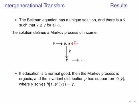
I The Bellman equation has a unique solution, and there is a ysuch that y ≤ y for all α.
The solution defines a Markov process of income.
y e,α
y
h
ν
· · ·
I If education is a normal good, then the Markov process isergodic, and the invariant distribution µ has support on [0, y],where y solves h
(1, e∗(y)
)= y.
85 / 150

Intergenerational Transfers Redistribution
An education-specific tax policy taxes each individual as a functionof their education and their income. It is redistributive if theaggregate tax collection is 0 for every education level e.
Tax policy τ1 is more egalitarian than tax policy τ2 iff thedistribution of income under τ2 is riskier than that of τ1 conditionalon the education level e.I If τ1 and τ2 are redistributive educational tax policies, and τ1
is more egalitarian than τ2, then for all income levels y,V∗τ1
(y) > V∗τ2(y).
I A result about universal public education.I A result on the relationhip between ability and earnings.
86 / 150

Trust
Three Stories about Trust:
Reciprocity: Reputation games, folktheorems, . . .
Social Learning: Generalized trust.
Behavioral Theories: Evolutionary Psychology, prosocialpreferences, . . .
87 / 150

Inequality and Trust
I Evidence for a correlation between trust and incomeinequality
I Rothstein and Uslaner (2005), Uslaner and Brown (2005).
I Trust is correlated with optimism about one’s own life chancesI Uslaner (2002)
88 / 150

Networks, Trust, and Development
I Informal social organization substitutes for markets and formalsocial institutions in underdeveloped economies.
I In the US, periods of high growth have also been periods ofdecline in social capital (Putnam, 2000)
I Possibly: Social capital is needed for economic developmentonly up to some intermediate stage, where generalized trustin institutions takes the place of informal trust arrangements.
89 / 150

Does Social Capital Have an Economic Payoff?
Knaak and Keefer (1997). “Does social capital have a payoff".
gi = Xiγ+ Ziπ+ CIVICiα+ TRUSTiβ+ εi
gi real per-capita growth rate.
Xi control variables — Solow.
Zi control variables — “endogenous” growth models.
CIVICi index of the level of civic cooperation.
TRUSTi the percentage of survey respondents (after omittingthose responding ‘don’t know’) who, when queriedabout the trustworthiness of others, replied that ‘mostpeople can be trusted’.
90 / 150

A Model of TrustI A population of N completely anonymous individuals.I Individuals have no distinguishing features, and so no one can
be identified by any other.I Individuals are randomly paired at each discrete date t , with
the opportunity to pursue a joint venture. Simultaneously withher partner, each individual has to choose whether toparticipate (P) in the joint venture, or to pursue anindependent venture (I). The entirety of her wealth must beinvested in one or the other option. The individual with wealthw receives a gross return wπ from her choice, where π isrealized from the following payoff matrix:
investor
partnerP I
P R rI e e
Gross Returns
91 / 150
A Model of Trust
I ER > Ee > Er .
I Individuals reinvest a constant fraction β of their wealth.
I Strategies for i are functions which map the history of isexperience in the game to actions in the current period.
I Equilibria: Always play P, always play I are two equilibria.
92 / 150

LearningEach individual i has a prior belief ρ, about the probability of one’sopponent choosing P. The prior distribution is beta withparameters a i, b i > 0. In more detail,
ρi(x) = β(a i0, b
i0)
=Γ(a i
0 + b i0)
Γ(a i0)Γ(b
i0)
xa i0−1(1 − x)b i
0−1.
Let ρit denote individual i’s posterior beliefs after t rounds of
matching. The posterior densities ρit and ρj
t will be conditioned ondifferent data, since all information is private. The updating rule forthe β distribution has
ρit (ht ) ≡ β(a i
t , bit ) = β(a i
0 + n, b i0 + t − n)
for histories containing n P ’s and therefore t − n I’s. The posteriormean of the β distribution is a i
t /(ait + b i
t ).93 / 150

Optimal Play
q∗ = (e − r)/(R − r)
I Let mit denote i’s mean of ρt .
I An optimal strategy for individual i is: Choose P if mt > q∗ andchoose I otherwise.
Theorem 3: For all initial beliefs (ρ10, . . . , ρ
N0 ), almost surely either
limt nPt = 0 or limtnP
t = N. The probabilities of both are positive.The limit wealth distributions in both cases isPr limt wt > w ∼ cwk , where k is kP or kI, and kP < kI.
94 / 150

Social Learning
95 / 150

Averaging the Opinions of Others
I DeGroot (1974)
I X is some event. pi(t) is the probability that i assigns to theoccurance of X at time t .
I A is a stochastic matrix. aij is the weight i gives to j’s opinion.
I p(t) = Ap(t − 1) = · · · = A tp(0).
96 / 150
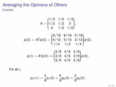
Averaging the Opinions of OthersExample
A =
1/3 1/3 1/31/2 1/2 0
0 1/2 1/2
,p(2) = A2p(0) =
5/18 8/18 5/185/12 5/12 2/121/4 1/2 1/4
p(0),
p(t) = A tp(0)→
3/9 4/9 2/93/9 4/9 2/93/9 4/9 2/9
p(0).
For all i,
pi(∞) =39
p1(0) +49
p2(0) +29
p3(0).
97 / 150

Averaging the Opinions of OthersDistinct Limits
A =
1/2 1/2 0 01/3 2/3 0 0
0 0 1/2 1/20 0 2/3 1/3
A t →
2/5 3/5 0 02/5 3/5 0 0
0 0 3/5 2/50 0 3/5 2/5
pi(t)→25
p1(0) +35
p2(0) for i = 1, 2.
pi(t)→35
p3(0) +25
p4(0) for i = 3, 4.
98 / 150

Averaging the Opinions of OthersNo Limit
A =
0 1 0 00 0 1 00 0 0 11 0 0 0
A t = A (t−1)mod 3+1
99 / 150

Averaging the Opinions of OthersConvergence
Theorem: If A is irreducible and aperiodic, then beliefs converge toa limit probability. For all j, limt→∞ pj(t) =
∑i ce
i pi(0), where ce isthe unit-normalized eigenvalue centrality of A .
100 / 150

Speed of ConvergenceHow long does it take for an individual’s belief to get near to thelimit belief?
∣∣∣pi(t) − pi(∞)∣∣∣ =
∣∣∣∣∣∣∣∣∑
j
A tij −
∑j
cej
pj(0)
∣∣∣∣∣∣∣∣For each j 0 < pj(0) < 1,
supp(0)
∣∣∣∣∣∣∣∣∑
j
A tij −
∑j
cej
pj(0)
∣∣∣∣∣∣∣∣ =max
∑
j:A tij≥ce
j
A tij −
∑j
cej
,− ∑j:A t
ij≤cej
A tij −
∑j
cej
=∣∣∣∣∣∣∣∣A t
ij − ce∣∣∣∣∣∣∣∣
TV
101 / 150

Speed of Convergence
For x and y in the non-negative unit simplex,
||x − y ||TV = supA|∑i∈A
(xi − yi)|.
We want to max this over individuals, so
d(t) = supi
∣∣∣∣∣∣∣∣A tij − ce
∣∣∣∣∣∣∣∣TV
.
Define
t(ε) = mint : d(t) < ε
t∗ = t(1/4).
102 / 150

A Lower Bound for t∗
Q(i, j) = cei Aij, Q(A ,B) =
∑i∈A j∈B
Q(i, j).
Q(A ,B) is the amount of influence B inherits from A .
Φ(S) =Q(S,Sc)∑
i∈S cei
, Φ∗ = infS :
∑i∈S ce
i ≤1/2Φ(S).
Φ(S) is the share of S ’s influence that is inherited by Sc .
Theorem: t∗ ≥1
4Φ∗.
103 / 150

Limit Beliefs and the “Wisdom of Crowds”
I Suppose that pi(0) = p + εi . The εi are all independent, havemean 0, and variances are bounded.
I What is the relationship between pi(∞) and p?I A sequence of networks (Vn,En)∞n=1, |Vn | = n, with centrality
vectors sn, and belief sequences pn(t).
Definition: The sequence learns if for all ε > 0,Pr
| limn→∞ limt→∞ pn(t) − p| > ε
= 0.
Theorem: If there is a B > 0 such that for all i, each individual’snormailzed centrality is less than B/n, then the sequence learns.I What conditions on the networks guarantee this?
104 / 150

Bayesian Learning on NetworksMulti-armed bandit problem
I An undirected network G.I Two actions, A and B. A pays off 1 for sure. B pays off 2 with
probability p and 0 with probability 1 − p.I At times t = 1, 2, . . ., each individual makes a choice, to
maximize E∑∞
τ=t βτπiτ|ht
, the expected present value of the
discounted payoff stream given the information.I p ∈ p1, . . . , pK . W.l.o.g. pj , pk and pk , 1/2.I Each individual has a full-support prior belief µi on the pk .I Individuals see the choices of his neighbors, and the payoffs.
105 / 150
Bayesian Learning on NetworksMulti-armed bandit problem
I If the network contains only one member, this is the classicmulti-armed bandit problem.
I How does the network change the classic results?I What does one learn from the behavior of others?
Theorem: With probability one, there exists a time such that allindividuals in a component play the same action from that time on.
I In one-individual problem, it is possible to lock into A when Bis optimal. How does the likelihood of this change in anetwork?
106 / 150

Bayesian Learning on NetworksCommon Knowledge
(Ω,F , p) A probability space.
X A finite set of actions.
Yi A finite set of signals observed by i. yi : Ω → Yk isF -measurable.
σ(f) If f is a measurable mapping of Ω into any measurespace, σf is the σ-algebra generated by f . Defineσ(yk ) = Yk .
Definition: A decision function maps states Ω to actions X . Adecision rule maps σ-fields on Ω to decision rules, that is,d(G) : Ω → X . For any σ-field G, d(G) is G-measurable. That is,σd(G) ⊂ G.
107 / 150

Bayesian Learning on NetworksCommon Knowledge
I Updating of beliefs:
Fk (t + 1) = Fk (t) ∨∨j,k
σd (Fj(t)) ,
Fk (0) = Yk .
Key Property: If σd(G) ⊂ H ⊂ G, then d(G) = d(H).
108 / 150

Bayesian Learning on NetworksCommon Knowledge
Theorem: Suppose d has the key property. Then there areσ-algebras Fk ⊂
∨k Yk and T ≥ 0 such that Fk (t) = Fk for all
t ≥ T , and for all k and j,
d(Fk ) = d(Fj) = d
∧i
Fi
.If the decision functions for all individuals are common knowledge,then they agree.
109 / 150

Bayesian Learning on NetworksCommon Knowledge
Now given is a connected undirected network (V ,E).I Individuals i and k communicate directly if there is an edge
connecting them.I Individuals i and k communicate indirectly if there is a path
connecting them.
Key Network Property: For any sequence of individualsk = 1, 2, . . . , n, if σd(Fk ) ⊂ Fk+1 and σd(Fn) ⊂ F1, thend(Fk ) = d(F1) for all k .
110 / 150

Bayesian Learning on Networks
Updating of beliefs:
Fk (t + 1) = Fk (t) ∨∨j∼k
σd (Fj(t)) ,
Fk (0) = Yk .
Theorem: Suppose d has the key network property. Then thereare σ-algebras Fk ⊂
∨k Yk and T ≥ 0 such that Fk (t) = Fk for all
t ≥ T , and for all k and j,
d(Fk ) = d(Fj) = d
∧i
Fi
.
111 / 150

Diffusion
112 / 150

Network Effects and Diffusion
113 / 150

Varieties of Action
I Graphical Games — Diffusion of actionI Blume (1993, 1995) — LatticesI Morris (2000) — General graphsI Young and Kreindler (2011) — Learning is fast
I Social Learning — Diffusion of knowledgeI Banerjee, QJE (1992)I Bikchandani, Hershleifer and Welch (1992)I Rumors
114 / 150

Coordination Games
A BA a,a 0,0B 0,0 b,b
Pure coordination game
a, b > 0
Three equilibria:⟨a, a
⟩,
⟨b, b
⟩, and
⟨( ba + b
,a
a + b
),( ba + b
,a
a + b
)⟩
115 / 150

Coordination Games
A BA a,a 0,0B 0,0 b,b
Pure coordination game
a, b > 0
Best response dynamics
% B0 1a/(a+b)
115 / 150

Coordination Games
A BA a,a d,cB c,d b,b
General coordination game
a > c, b > d
Here the symmetric mixed equilibrium is atp∗ = (b − d)/(a − c + b − d).
Suppose b − d > a − c. Then p∗ > 1/2. At (1/2, 1/2), A is thebest response. This is not inconsistent with b > a.
I A is Pareto dominant if a > b.I B is risk dominant if b − d < a − c.
116 / 150

Coordination Games — Stochastic Stability
Continuous time stochastic processI Each player has an alarm clock. When it goes off, she makes
a new strategy choice. The interval between rings has anexponential distribution.
I Strategy revision:I Each individual best-responds with prob. 1 − ε, Kandori,
Mailath and Robb (1993); Young (1993)or
I The log-odds of choosing A over B is proportional to the payoffdifference — logit choice, Blume (1993, 1995).
117 / 150

The Stochastic Process
This is a Markov process on the state space [0, . . . ,N], where thestate is the number of players choosing B.
Logit Choice Mistakes
In both cases, as Probbest response ↑ 1, ProbN ↑ 1.
118 / 150

Coordination on Networks
I Is the answer the same on every graph?
.
119 / 150

Coordination on Networks
I Is the answer the same on every graph?
Mistake: 0 : 0.5 N : 0.5. Logit: N : 1.
119 / 150

General Analysis
I In general, the strategy revision process is an ergodic Markovprocess.
I There is no general characterization of the invariantdistribution.
I The answer is well-understood for potential games and logitupdating.
120 / 150

A General Diffusion Model
I Best response strategy revision. If fraction q or more of yourneighbors choose A , then you choose A .
I Two obvious equilibria: All A and All B.
I How easy is it to “tip” from one to the other? What aboutintermediate equilibria?
121 / 150
A General Diffusion Model
I Imagine that everyone initially uses B.
I Now a small group adopts A .
I When does it spread, when does it stop?
I The answer should depend on the network structure, who arethe initial adopters, and the threshold p∗.
122 / 150

Diffusion of Coordination — Line
When the Poisson alarm clock rings, the player best responds tohis neighbors. p∗ < 1/2. Questions:I Are islands of risk dominance stable?I Can risk dominance spread?
123 / 150

Diffusion of Coordination — Line
When the Poisson alarm clock rings, the player best responds tohis neighbors. p∗ < 1/2. Questions:I Are islands of risk dominance stable?I Can risk dominance spread?
123 / 150

Diffusion of Coordination — Line
When the Poisson alarm clock rings, the player best responds tohis neighbors. p∗ < 1/2. Questions:I Are islands of risk dominance stable?I Can risk dominance spread?
123 / 150

Diffusion of Coordination — Line
When the Poisson alarm clock rings, the player best responds tohis neighbors. p∗ < 1/2. Questions:I Are islands of risk dominance stable?I Can risk dominance spread?
123 / 150
Diffusion of Coordination — Lattices
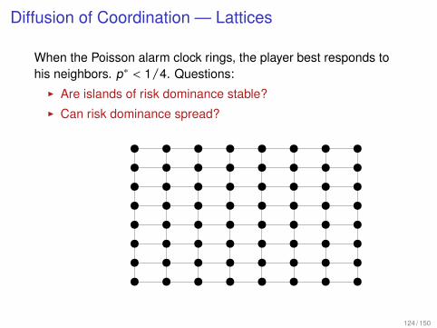
When the Poisson alarm clock rings, the player best responds tohis neighbors. p∗ < 1/4. Questions:I Are islands of risk dominance stable?I Can risk dominance spread?
124 / 150

Diffusion of Coordination — Lattices
When the Poisson alarm clock rings, the player best responds tohis neighbors. p∗ < 1/4. Questions:I Are islands of risk dominance stable?I Can risk dominance spread?
124 / 150

Diffusion of Coordination — Lattices
When the Poisson alarm clock rings, the player best responds tohis neighbors. p∗ < 1/4. Questions:I Are islands of risk dominance stable?I Can risk dominance spread?
124 / 150

Diffusion of Coordination — Lattices
When the Poisson alarm clock rings, the player best responds tohis neighbors. p∗ < 1/4. Questions:I Are islands of risk dominance stable?I Can risk dominance spread?
124 / 150

Diffusion of coordination — General Graphs
I A cluster of density p is a set of vertices C such that for eachv ∈ C, at least fraction p of v ’s neighbors are in C.
The set C = A ,B,C is a cluster of density 2/3.
A
B C
125 / 150

General Graphs
Two observations:
I Every graph will have a cascade threshold.
I If the initial adoptees are a cluster of density at least p∗, thendiffusion can only move forward.
126 / 150

General Graphs: Clusters Stop Cascades
Consider a set S of initial adopters in a network with vertices T ,and suppose that remaining nodes have threshold q.
Claim: If Sc contains a cluster with density greater than1 − q, then S will not cause a complete cascade.
Proof: If there is a set T ⊂ Sc with density greater than1 − q, then even if S/T chooses A , every member ofT has fraction more than 1 − q choosing B, andtherefore less than fraction q are choosing A .Therefore no member of T will switch.
127 / 150

General Graphs: Clusters Stop Cascades
Claim: If a set S ⊂ V of initial adopters of an innovation withthreshold q fails to start a cascade, then there is acluster C ∈ V/S of density greater than 1 − q.
Proof: Suppose the innovation spreads from S to T andthen gets stuck. No vertex in Tc wants to switch, soless than a fraction q of its neighbors are in T , morethan fraction 1 − q are out. That is Tc has densitygreater than 1 − q.
128 / 150

Networks and OptimalityI Networks make it easier for cascades to take place.
I In the fully connected graph, a cascade from a small groupnever takes place. With stochastic adjustment in the mistakesmodel, the probability of transiting from all A to all B is O(εqN),where q is the indifference threshold. On a network, theprobability of transiting from all A to all B is on the order of εK ,where K is the size of a group needed to start a cascade, andthis is independent of N.
I This is not always optimal!
I Risk dominance and Pareto dominance can be different. Thiscan be understood as a robustness question. If the populationhas correlated on the efficient action, how easy is it to undo?Hard if the efficient action is risk dominant. If the efficientaction is not risk-dominant, it is easier to undo on sparsenetworks than on nearly completely connected networks.
129 / 150

Community Structure
Under Construction
130 / 150

Two Problems
Imagine a social network, such as a friendship network in a schoolor network of information sharing in a village. Suppose the networkparticipants represent several ethnic groups, races or tribes.
I How “integrated” is the network with respect to predefinedcommunities?
I What are the implicit “comunities” of highly mutuallyinteractive neighbors?
I How do these community structures map onto each other?
131 / 150

Measuring Segregation
Attributes of physical segregation.
I Evenness — Differentialdistribution of two groups acrossthe network.
I Exposure — The degree to whichdifferent groups are in contact.
I Concentration — Relativeconcentration of physical spaceoccupied by different groups.
132 / 150

Measuring Segregation
Attributes of physical segregation.
I Centraliztion — Extent to which agroup is near the center.
I Clustering — Degree to whichgroup members are connected toothers in the group.
132 / 150

Dissimilarity Index
A city is divided into N areas. Area i hasminority population mi and majoritypopulation Mi . Total populations are m andM, respectively.
dissimilarity index =12
N∑i=1
∣∣∣∣∣∣mi
m−
Mi
M
∣∣∣∣∣∣.frac. M
frac. m
133 / 150

References: Introduction I
Asch, Solomon E. 1951. “Effects of group pressure on themodification and distortion of judgements.” In Groups,Leadership and Men, edited by H. Guetzkow. Pittsburgh:Carnegie Press.
Baker, Wayne E. 1984. “The Social Structure of a NationalSecurities Market.” American Journal of Sociology89 (4):775–811.
Duesenberry, James S. 1960. “Comment on G. Becker, ‘Aneconomic analysis of fertility’.” In Demographic and EconomicChange in Developed Countries, edited by George B. Roberts.New York: Columbia University Press for the National Bureau ofEconomic Research, 231–34.
Glaeser, Edward L., Bruce Sacerdote, and Jose A. Scheinkman.1996. “Crime and Social Interaction.” Quarterly Journal ofEconomics 111 (2):507–48.
134 / 150

References: Introduction IIKandel, Denise B. 1978. “Homophily, selection, and socialization in
adolescent friendships.” American Journal of Sociology84 (2):427–36.
Mennis, Jeremy and Philip Harris. 2001. “Contagion and repeatoffending among urban juvenile delinquents.” Journal ofAdolescence 34 (5):951–63.
Polanyi, Karl. 1944. The Great Transformation. New York: Farrarand Rinehart.
Reiss Jr., Albert J. 1986. “Co-offending influences on criminalcareers.” In Criminal Careers and ‘Career Criminals’, vol. 2,edited by Alfred Blumstein, Jacqueline Cohen, Jeffrey A. Roth,and Christy A. Visher. Washington, DC: National AcademyPress, 121–160.
Sacerdote, Bruce I. 2001. “Peer effects with random assignmentresults for Dartmouth roommates.” Quarterly Journal ofEconomics 116 (2):681–704.
135 / 150

References: Introduction III
Sherif, M. et al. 1954/1961. Intergroup Conflict and Cooperation:The Robbers Cave Experiment. Norman: University ofOklahoma Book Exchange.
Warr, Mark. 1996. “Organization and instigation in delinquentgroups.” Criminology 34 (1):11–37.
136 / 150

References: Network Science I
Amaral, L. A. N., A. Scala, M. Barthélémy, and H. E. Stanley. 2000.“Classes of small-world networks.” Proc. Natl. Acad. Sci. USA.97:11149–52.
Bearman, Peter, James Moody, and Katherine Stovel. 2004.“Chains of affection: The structure of adolescent romantic andsexual networks.” American Journal of Sociology 110 (1):44–99.
Bonacich, Phillip. 1987. “Power and centrality: A family ofmeasures.” American Journal of Sociology 92 (5): 1170–1182.
Bonacich, Phillip and Paulette Lloyd. 2001. “Eigenvector-likemeasures of centrality for asymmetric relations.” SocialNetworks 23 (3): 191–201.
Christakis, Nicholas A. and James H. Fowler. 2007. “The spread ofobesity in a large social network over 32 years.” New EnglandJournal of Medicine 357:370–9.
137 / 150

References: Network Science II
Cohen-Cole, Ethan and Jason M. Fletcher. 2008. “Is obesitycontagious? Social networks vs. environmental factors in theobesity epidemic.” Journal of Health Economics 27 (5):1382–87.
Davis, Gerald F., Mina Yoo, and Wayne E. Baker. 2003. “The smallworld of the American corporate elite, 1982-2001.” StrategicOrganization 1 (3):301–26.
Eggenberger, F. and G. Polya. 1923. “Über die Statistik verketteterVorgänge”. Zeitschrift für Angewandte Mathematik undMechanik 3 (4): 279–289.
Gladwell, Malcom. 1999. “Six degrees of Lois Weisberg.” NewYorker, January 11.
Korte, Charles and Stanley Milgram. 1970. “Acquaintancenetworks between racial groups: Application of the small worldmethod.” Journal of Personality and Social Psychology15 (2):101–08.
138 / 150

References: Network Science IIIR. Kumar, P. Raghavan, S. Rajagopalan, D. Sivakumar, A.
Tomkins and E. Upfal. “Stochastic models for the web graph.”FOCS 2009.
Lazarsfeld, P. F. and R. K. Merton. 1954. “Friendship as socialprocess: A substantive and methodological analysis.” InFreedom anc Control in Modern Society, edited by MorroeBerger, Theodore Abel, and Charles H. Page. New York: VanNostrand, 18–66.
Liljeros, F., C.R. Edling, and L. Nunes Amaral. 2003. “Sexualnetworks: implications for the transmission of sexuallytransmitted infections.” Microbes and Infection 5 (2):189–96.
Milgram, Stanley. 1967. “The small world problem.” PsychologyToday 2:60–67.
Moody, James. 2001. “Race, school integration, and friendshipsegregation in America.” American Journal of Sociology107 (3):679–716.
139 / 150

References: Network Science IV
Newman, Mark E. J. 2003. “The structure and function of complexnetworks.” SIAM Review 45 (2):167–256.
Rappoport, Anatole. 1953. “Spread of information through apopulation with social-structural bias I: Assumption oftransitivity.” Bulletin of Mathematical Biophysics 15 (4):523–33.
Herbert A. Simon (1955). “On a class of skew distributionfunctions”. 55 (3–4): 425–440.
Travers, Jeffrey and Stanley Milgram. 1969. “An experimentalstudy of the small world problem.” Sociometry 32 (4):425–43.
Watts, D. J. and S. H. Strogatz. 1998. “Collective dynamics of“small-world” networks.” Nature 393:440–42.
G. K. Zipf. 1949. Human Behavior and the Principle of Least EffortAddison-Wesley, Cambridge, MA.
140 / 150

References: Labor MarketsCalvó-Armengol, Antoni and Matthew O. Jackson. 2004. “The
Effects of Social Networks on Employment and Inequality.”American Economic Review 94 (3):426–54.
Granovetter, M. S. 1973. “The Strength of Weak Ties.” AmericanJournal of Sociology 78 (6):1360–80.
Montgomery, James D. 1991. “Social networks and labor-marketoutcomes: Towards an economic analysis.” American EconomicReview 81 (5):1408–18.
Rapoport, A. and W. Horvath. 1961. “A study of a largesociogram.” Behavioral Science 6:279–91.
Scotese, Carol A. 2012. “Wage inequality, tasks and occupations.”Unpublished, Virginia Commonwealth University.
Tian, Felicia and Nan Lin. 2016. “Weak ties, strong ties, and jobmobility in urban China.” Social Networks 44:117–29.
Yakubovich, Valery. 2005. “Weak ties, information, and influence:How workers find jobs in a local Russian labor market.”American Sociological Review 70 (3):408–21.
141 / 150

References: Matching I
Blume, Lawrence, David Easley, Jon Kleinberg, Bobby Kleinbergand Éva Tardos. 2013. “Network formation in the presence ofcontagious risk.” ACM Transactions on Economics andComputation 1 (2).
Jackson, Matthew O. and Asher Wolinsky. 1996. “A strategic modelof network formation.” Journal of Economic Theory 71:44–74.
Gale, David and Lloyd Shapley. 1962. “College admissions and thestability of marriage.” American Mathematical Monthly 69:9–14.
Shapley, Lloyd and Martin Shubik. 1972. “The assignment game I:The core.” International Journal of Game Theory 1: 111–130.
142 / 150

References: Peer Effects and Complementarities I
Blume, L., W. Brock, S. Durlauf, and Y. Ioannides. 2011.“Identification of Social Interactions.” In Handbook of SocialEconomics, vol. 1B, edited by J. Benhabib, A. Bisin, andM. Jackson. Amsterdam: North Holland, 853–964.
Blume, Lawrence E., William Brock, Steven N. Durlauf, and RajshriJayaraman. 2013. “Linear Social Interaction Models.” Journal ofPoliical Economy 123 (2):444–96.
Durlauf, Steven N. 2004. “Neighborhood effects.” In Handbook ofRegional and Urban Economics, edited by J. V. Henderson andJ. F. Thisse. Amsterdam: Elsevier, 2173–2242.
Ioannides, Yannis M. and Giorgio Topa. 2010. “Neighborhoodeffects: Accomplishments and looking beyond them.” Journal ofRegional Science 50 (1):343–62.
143 / 150

References: Peer Effects and Complementarities II
Hoxby, Caroline M. and Gretchen Weingarth. 2005. “Taking raceout of the equation: School reassignment and the structure ofpeer effects.” NBER Working Paper.
Manski, Charles F. 1993. “Identification of Endogenous SocialEffects: The Reflection Problem.” Review of Economic Studies60:531–42.
Sacerdote, B. 2011. “Peer effects in education: How might theywork, how big are they and how much do we know thus far?”Handbook of the Economics of Education 3:249–277.
144 / 150

References: Social Capital I
Bourdieux, P. and L. J. D. Wacquant. 1992. An Invitation toReflexive Sociology. Chicago, IL: University of Chicago Press.
Fukuyama, Francis. 1996. Trust: Social Virtues and the Creation ofProsperity. New York: Simon and Schuster.
Knaak, Stephen and Philip Keefer. 1997. “Does Social CapitalHave an Economic Payoff? A Cross-Country Investigation.”Quarterly Journal of Economics 112 (4):1251–88.
Lin, Nan. 2001. Social Capital. Cambridge UK: CambridgeUniversity Press.
Loury, Glenn. 1992. “The economics of discrimination: Getting tothe core of the problem.” Harvard Journal for African-AmericvanPublic Policy 1:91–110.
Portes, Alejandro. 1998. “Social capital: Its origins and applicationsin modern sociology.” Annual Review of Sociology 24:1–24.
145 / 150

References: Social Capital II
Putnam, Robert. 2000. Bowling Alone: The Collapse and Revivalof American Community. New York: Simon and Schuster.
Putnam, Robert D. 1995. “Bowling alone: America’s decliningsocial capital.” Journal of Democracy 6:65–78.
Rothstein, B. and Eric M. Uslaner. 2005. “All for all: Equality,corrpution, and social trust.” World Politics 58 (1):41–72.
Uslaner, Eric M. 2002. The Moral Foundations of Trust. CambridgeUK: Cambridge University Press.
Uslaner, Eric M. and M. Brown. 2005. “Inequality, trust, and civicengagement.” American Politics Research 33 (6):868–94.
146 / 150

References: Social Learning
Bala, Venkatesh and Sanjeev Goyal. 1996. “Learning fromneighbors.” Review of Economic Studies 65:595-621.
Banerjee, Abhijit V. 1992. “A simple model of herd behavior.”Quarterly Journal of Economics 107 (3):797–817.
Bonacich, Phillip. 1987. “Power and centrality: A family ofmeasures.” American Journal of Sociology 92 (5):1170–82.
Bonacich, Phillip and Paulette Lloyd. 2001. “Eigenvector-likemeasures of centrality for asymmetric relations.” SocialNetworks 23:191–201.
DeGroot, Morris H. 1974. “Reaching a consensus.” Journal of theAmerican Statistical Association 69:118–21.
Jackson, Matthew O. and Benjamin Golub. 2010. “Naive learningin social networks and the wisdom of crowds.” AmericanEconomic Journal: Microeconomics 2 (1):112-49.
147 / 150

References: Diffusion
Blume, Lawrence E. 1993. “The statistical mechanics of strategicinteraction.” Games and Economic Behavior 5 (5):387–424.
———. 1995. “The statistical mechanics of best-response strategyrevision.” Games and Economic Behavior 11 (2):111–145.
Kandori, Michihiro, George J. Mailath and Rafael Robb. 1993.“Learning, mutation, and long run equilibria in games.”Econometrica 61 (1):29–56.
Morris, Stephen. 2000. “Contagion.” Review of Economic Studies67 (1):57–78.
Young, H. Peyton. 1993. “The evolution of convention.”Econometrica 61 (1): 29–56.
——— and Gabriel H. Kreindler. 2011. “Fast Convergence inevolutionary equilibrium selection.” Oxford EconomicsDiscussion Paper No. 569.
148 / 150

References: Community Structure
Massey, Douglas and Nancy Denton. 1988. “The dimensions ofresidential segregation.” Social Forces 67:281–315.
149 / 150

References: General
Easley, David A. and Jon Kleinberg. 2010. Networks, Crowds andMarkets: Reasoning About a Highly Connected World.Cambridge UK: Cambridge University Press.
Jackson, Matthew O. 2008. Social and Economic Networks.Princeton University Press.
150 / 150