economic report on order duplication and liquidity measurement in
TRANSCRIPT

Order duplication and liquidity measurement in EU equity markets
ESMA Economic Report No. 1, 2016

ESMA Economic Report No. 1, 2016 2
ESMA Economic Report, Number 1, 2016
Contributors: Carlos Aparicio Roqueiro, Claudia Guagliano, Cyrille Guillaumie, Steffen Nauhaus, Christian Winkler, Steffen Kern.
Acknowledgements: We thank the members of the CEMA HFT Task Force, namely Annemarie Pidgeon, Bas Verschoor, Carla Cabrita, Carla Ysusi, Carole Gresse, Christophe Majois, Felix Suntheim, Giovanni Siciliano, Julien Leprun, Kheira Benhami, Luc Goupil, Marc Ponsen, Nicolas Megarbane, Ramiro Losada, Richard Payne, Hans Degryse, Rudy de Winne, Sander van Veldhuizen, Thorsten Freihube, Valeria Caivano, Victor Mendes for helpful suggestions. We are grateful to Antoine Bouveret for his early leadership of this research project, his conceptual input, as well as his valuable comments.
Authorisation: This Report has been reviewed by ESMA’s Committee for Economic and Market Analysis (CEMA) and has been approved by the Authority’s Board of Supervisors.
© European Securities and Markets Authority, Paris, 2016. All rights reserved. Brief excerpts may be reproduced or translated provided the source is cited adequately. Legal reference of this Report: Regulation (EU) No 1095/2010 of the European Parliament and of the Council of 24 November 2010 establishing a European Supervisory Authority (European Securities and Markets Authority), amending Decision No 716/2009/EC and repealing Commission Decision 2009/77/EC, Article 32 “Assessment of market developments”, 1. “The Authority shall monitor and assess market developments in the area of its competence and, where necessary, inform the European Supervisory Authority (European Banking Authority), and the European Supervisory Authority (European Insurance and Occupational Pensions Authority), the ESRB and the European Parliament, the Council and the Commission about the relevant micro-prudential trends, potential risks and vulnerabilities. The Authority shall include in its assessments an economic analysis of the markets in which financial market participants operate, and an assessment of the impact of potential market developments on such financial market participants.”
European Securities and Markets Authority (ESMA) Economics and Financial Stability Unit 103, Rue de Grenelle FR–75007 Paris [email protected]
ESMA Economic Report No. 1, 2016 3
Table of contents
Executive summary .................................................................................................. 4
Introduction .............................................................................................................. 5
Literature review....................................................................................................... 7
Dataset description ................................................................................................ 10
Identifying high-frequency trading – the key results of ESMA (2014) ............... 12
The extent of order duplication in EU equity markets ........................................ 14
The behaviour of trade participants ..................................................................... 17
Impact of trading on gross and net liquidity ........................................................ 18
Conclusion .............................................................................................................. 23
References .............................................................................................................. 25
Annex 1: Sample characteristics .......................................................................... 27
Annex 2: Impact of trading on gross and net liquidity- additional results ........ 29

ESMA Economic Report No. 1, 2016 4
Executive summary
This report is the second part of ESMA’s high-frequency trading (HFT) research. The starting point for both reports is the change in the trading landscape of equity markets over the last decade. The defining features of this change are increased competition between trading venues, fragmentation of trading of the same financial instruments across EU venues and the increased use of fast and automated trading technologies. In our first report we analysed the extent of HFT activity across the EU in such an environment using a novel identification method for HFT activity. We found that HFT activity represents between 24% and 43% of value traded and between 58% and 76% of orders in our sample.1 In this report we focus on liquidity measurement where equity trading is fragmented.
In an environment characterised by competition between trading venues, traders do not always know on which venue they will be able to trade. They may “advertise” their intention to trade by posting similar orders on more than one trading venue at the same time (“duplicated orders”). This, however, leads to the risk of trading more shares than wanted. Therefore some traders may immediately cancel unmatched duplicated orders on other venues after one of their duplicated orders has been filled.
Using the HFT identification method developed in our first report, we find evidence for this trading pattern. 20% of the orders in our sample are duplicated orders and in 24% of trades the trader immediately cancels unmatched duplicated orders. We believe that duplication of orders and immediate cancellation of duplicates after a trade has become part of the strategy to ensure execution in fragmented markets, e.g. for market makers or where institutional investors are searching for liquidity. However, we show that taking duplicated orders into account when measuring liquidity leads to overestimation of available liquidity in fragmented markets.
The proportion of duplicated orders varies with the type of traders, the market capitalisation of the underlying stock and the fragmentation of trading in a stock. As expected, duplicated orders are more prevalent for HFTs (34% of orders) than for non-HFTs (12% of orders). They account for 22% of orders in large cap stocks compared to 12% of orders in small cap stocks. Also, fragmentation of trading is positively correlated with order duplication. We find 13% of duplicated orders for stocks with low trading fragmentation and 23% for high fragmentation.
Regarding the extent to which duplicated orders are immediately cancelled after trades (and thus subsequently are not available to the market), we carry out a number of analyses. First, we find that for 24% of all trades, the trader on the passive side of the trade immediately cancels order duplicates after the trade. This proportion is higher for HFTs (28%), large cap stocks (27%) and where trading is more fragmented (31%). Second, we look at the different reaction of two measures of liquidity: gross liquidity, the aggregated volume of displayed orders across multiple markets, and net liquidity, which deducts duplicated orders from the gross liquidity measure. We compare these two measures to establish whether order duplication should be taken into account when measuring liquidity in fragmented markets. A stronger fall of the gross liquidity measure after trades compared to the net liquidity measure is an additional indication that a proportion of duplicated orders is indeed immediately cancelled after trades and thus not available to the market. Our descriptive and econometric analyses confirm this hypothesis.
Both in our first HFT report and in this report we use unique data collected by ESMA, covering a sample of 100 stocks on 12 trading venues in nine EU countries for May 2013. Our data allow us to identify market participants’ actions across different venues. Thus we are able to complement the literature, as most of the HFT studies published so far focus either on the US or on a single country within Europe and few are able to analyse the behaviour of market participants across trading venues.
Previous studies have found evidence supporting that fragmentation of trading increases liquidity in equity markets. Our analysis qualifies these results, as using data that allow us to identify market participants’ actions across different venues, we find a substantial extent of order duplication in fragmented markets. It is important to state that unless they are successfully cancelled, duplicated orders are available to the market and all of them can be matched. However we find that a substantial proportion of order duplicates are immediately cancelled after a trade occurs and thus subsequently not available to the market. From an analytic perspective, our findings suggest that to avoid overestimation of available liquidity duplicated orders should be taken into account when measuring liquidity in fragmented markets, for example with our net liquidity measure.
1 https://www.esma.europa.eu/sites/default/files/library/2015/11/esma20141_-_hft_activity_in_eu_equity_markets.pdf

ESMA Economic Report No. 1, 2016 5
Introduction
In recent years, financial markets have undergone
a series of significant changes. Regulatory
developments, technological innovation and
growing competition have increased the
opportunities to employ innovative infrastructures
and trading practices.
On the regulatory side, the entry into force of the
Market in Financial Instruments Directive (MiFID)
in 2007 has re-shaped markets in the EU.
Simultaneously, developments in new
technologies have enabled the use of automated
and very fast trading technologies.2 The resulting
trading landscape can be characterised by higher
competition between trading venues, the
fragmentation of trading in the same financial
instruments across venues in the EU, as well as
the increased use of fast and automated trading
technologies.
It has been suggested that the order books of
exchanges are today less informative than
previously since liquidity is more transitory or “less
certain”, as in fragmented markets it is not easy to
anticipate where potential counterparties will trade
next, or if they are active only on one venue or on
multiple venues. Lescourret and Moinas (2015)
analyse liquidity supply in fragmented financial
markets and find that ex ante fragmentation may
decrease total transaction costs (a measure of
market liquidity): The possibility to compete in a
single venue forces in some cases competitors to
post aggressive quotes across all venues.
In this context, the disparity in terms of speed and
technology between ordinary traders and high-
frequency traders (HFTs) has become significant.
Investment in fast trading technology helps
financial institutions cope with market
fragmentation (Biais et al, 2015). Thus,
fragmentation may be more likely to attract HFTs,
as they are able to implement cross-venue
arbitrage strategies.
At the same time, recent events of short-term
liquidity shortages and sudden spikes of volatility
across market segments have triggered questions
related to the impact of HFT on volatility, liquidity
and, more generally, market quality.
When it comes to analysing the impact of HFT
activity the operational definition of HFT becomes
crucial. In general, total trading activity can be
divided into algorithmic trading (AT) and non-
2 See e.g. Lo (2016) for an overview of technological
change in finance.
algorithmic trading, depending on whether or not
market participants use algorithms to make trading
decisions without human intervention. Kirilenko
and Lo (2013), for example, describe AT as “the
use of mathematical models, computers, and
telecommunications networks to automate the
buying and selling of financial securities”.3
Following definitions proposed in the literature,
HFT is a subset of AT and has the following
features
— proprietary trading;
— very short holding periods;
— submission of a large number of orders that
are cancelled shortly after submission;
— neutral positions at the end of a trading day;
and
— use of colocation and proximity services to
minimise latency.
From an analytical perspective, the absence of a
unique definition makes it difficult to achieve a
precise identification of HFT activity. The literature
employs a number of approaches to identify HFT
activity. None of these approaches is able to
exactly capture HFT activities and they lead to
widely differing levels of HFT activity. In 2014,
ESMA published a report discussing the
identification of HFT and providing estimates of
HFT activity based on a cross-EU sample of
stocks. The report, using unique data collected by
ESMA covering a sample of 100 stocks from 9 EU
countries and 12 trading venues for May 2013,
shed further light on the extent of HFT in EU equity
markets. The report provided a lower and an upper
bound for HFT activity, employing two main
methodologies:
a) direct approach: an institution based measure
(each institution is either HFT or not) focusing
on the primary business of firms (lower
bound), and
3 A legal definition of algorithmic trading is provided by
MiFID II. Article 4(1)(39) of MiFID II states that algorithmic trading “means trading in financial instruments where a computer algorithm automatically determines individual parameters of orders such as whether to initiate the order, the timing, price or quantity of the order or how to manage the order after its submission, with limited or no human intervention, and does not include any system that is only used for the purpose of routing orders to one or more trading venues or for the processing of orders involving no determination of any trading parameters or for the confirmation of orders or the post-trade processing of executed transactions”. http://eur-lex.europa.eu/legal-content/EN/TXT/PDF/?uri=CELEX:32014L0065&from=EN
ESMA Economic Report No. 1, 2016 6
b) indirect approach: a stock-based measure (an
institution may be HFT for one stock but not
for another one) focusing on the lifetime of
orders (upper bound).4
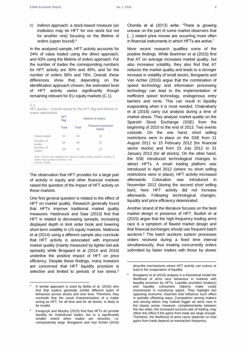
In the analysed sample, HFT activity accounts for
24% of value traded using the direct approach,
and 43% using the lifetime of orders approach. For
the number of trades the corresponding numbers
for HFT activity are 30% and 49%, and for the
number of orders 58% and 76%. Overall, these
differences show that, depending on the
identification approach chosen, the estimated level
of HFT activity varies significantly though
remaining relevant for EU equity markets (C.1).
C.1 HFT activity – Overall results for the HFT flag and lifetime of orders approaches
HFT flag
Lifetime of orders
Total Total
Thereof investment banks
Value traded 24 43 22
Number of trades
30 49 23
Number of orders
58 76 19
Note: Figures are weighted by value of trades (value traded), number of trades and number of orders, in %. Source: ESMA.
The observation that HFT provides for a large part
of activity in equity and other financial markets
raised the question of the impact of HFT activity on
these markets.
One first general question is related to the effect of
HFT on market quality. Research generally found
that HFTs improve traditional market quality
measures: Hasbrouck and Saar (2013) find that
HFT is related to decreasing spreads, increasing
displayed depth in limit order book and lowering
short-term volatility in US equity markets. Malinova
et al (2014) using a different sample also conclude
that HFT activity is associated with improved
market quality (mainly measured by tighter bid-ask
spreads) while Brogaard et al (2014 and 2016)
underline the positive impact of HFT on price
efficiency. Despite these findings, many investors
are concerned that HFT liquidity provision is
selective and limited to periods of low stress.5
4 A similar approach is used by Bellia et al. (2016) who
find that traders generally exhibit different types of behaviour across stocks and over time. Therefore, they conclude that the usual characterisation of a trader acting as HFT, for all time and for all stocks, is likely to be invalid.
5 Korajzcyk and Murphy (2015) find that HFTs do provide liquidity for institutional trades, but to a significantly smaller extent when trades are stressful, i.e. comparatively large. Bongaerts and Van Achter (2016)
Chordia et al (2013) write: “There is growing
unease on the part of some market observers that
[…] violent price moves are occurring more often
in financial instruments in which HFTs are active.”
More recent research qualifies some of the
positive findings. While Boehmer et al (2015) find
that AT on average increases market quality, but
also increases volatility, they also find that AT
reduces the market quality and leads to a stronger
increase in volatility of small stocks. Bongaerts and
Van Achter (2016) argue that the combination of
speed technology and information processing
technology can lead to the implementation of
inefficient speed technology, endogenous entry
barriers and rents. This can result in liquidity
evaporating when it is most needed. Chakrabarty
et al (2016) carry out analysis during a time of
market stress. They analyse market quality on the
Spanish Stock Exchange (SSE) from the
beginning of 2010 to the end of 2013. Two events
coincide: On the one hand, short selling
restrictions were in place on the SSE from 11
August 2011 to 15 February 2012 (for financial
sector stocks) and from 23 July 2012 to 31
January 2013 (for all stocks). On the other hand,
the SSE introduced technological changes to
attract HFTs. A smart trading platform was
introduced in April 2012 (where no short selling
restrictions were in place), HFT activity increased
afterwards. Colocation was introduced in
November 2012 (during the second short selling
ban); here HFT activity did not increase
afterwards. Following technological changes,
liquidity and price efficiency deteriorated.
Another strand of the literature focuses on the best
market design in presence of HFT. Budish et al
(2015) argue that the high-frequency trading arms
race is a symptom of flawed market design and
that financial exchanges should use frequent batch
auctions.6 The batch auctions system processes
orders received during a fixed time interval
simultaneously, thus treating concurrently orders
submitted by faster traders with those by slower
describe mechanisms where HFT activity can reduce or lead to the evaporation of liquidity.
6 Bongaerts et al (2016) analyse in a theoretical model the likelihood of arms race behaviour in markets with liquidity provision by HFTs. Liquidity providers (makers) and liquidity consumers (takers) make costly investments in monitoring speed. They highlight two opposing economic channels that influence such effect in partially offsetting ways. Competition among makers and among takers may indeed trigger an arms race in the classic sense. However, complementarity between the two sides, the increased success rate of trading, may offset this effect if the gains from trade are large enough. Therefore, the likelihood of arms races depends on how gains from trade depend on transaction frequency.

ESMA Economic Report No. 1, 2016 7
traders and reducing the benefit of marginal
superiority in speed.
Other researchers argue that HFTs are a
heterogeneous group and they employ a variety of
strategies, with different impact on financial
markets. Menkveld (2013) focuses on just one
HFT following a market making strategy and
shows the relationship between market
fragmentation and HFT in current financial
markets. Indeed, he shows how the HFT entry into
a large incumbent market NYSE-Euronext and the
entrant market Chi-X at the same time not only
fragmented trading, but it also coincided with a
50% drop in the bid-ask spread. Hagstromer and
Norden (2013) distinguish between HFTs following
market making strategies and others following
opportunistic strategies and show that the latter
are associated with increases in volatility, whereas
the former are associated with decreases in
volatility.
One of the concerns often mentioned with respect
to HFTs is that they overload the exchanges with
submissions and cancellations of limit orders,7
even though this strategy can be essential in
current fragmented market.
In this report we focus exclusively on the presence
of duplicated orders across multiple venues and
how this may affect the accurate measurement of
genuine liquidity and thus the accurate
understanding of liquidity dynamics.
We define duplicated orders as those posted on
the same side of the order book, at the same price
and by the same market agent but on different
venues. Our hypothesis is that order duplication is
partially explained by the search for counterparties
in fragmented markets8 and that, once the trading
objective has been fulfilled in one venue, in many
cases the liquidity will be immediately removed
from the other venues. Such a strategy requires
fast reaction, thus it is likely that mostly HFTs are
able to act in this way. This fast disappearance of
orders will have an impact on observed market
liquidity. The SEC’s Concept Release on Equity
Market Structure (2010) recognised the
importance of high frequency quoting in that it
might represent “phantom liquidity (which)
disappears when most needed by long-term
investors”. If this is the case, a liquidity measure
that takes account of the existence and the extent
7 See Egginton et al (2014), Friedrich and Payne (2015)
for more analysis on the impact of quote stuffing and high order-to trade-ratios on financial markets.
8 See AFM (2016) for a discussion based on interviews with market participants (HFT and buy-side firms as well as trading venues).
of order duplication should be more accurate than
a gross measure of liquidity that does not control
for order duplication.9 Conrad et al (2015) describe
the disadvantage characterising most of the
literature focusing on a single stock exchange: In a
fragmented market it is entirely possible that HFT
behaviour in one market may not reflect aggregate
market behaviour.10 Our unique dataset allows us
to avoid this disadvantage.
The structure of the paper is as follows. First, we
provide an overview of the existing literature on
the impact of HFT activity and fragmentation on
liquidity in financial markets. Second, we
describe our unique dataset. Then, we introduce
the duplicated orders metric which is based on
the concepts of gross and net liquidity.
We also analyse the behaviour of the different
traders performing the order duplication strategy
after the execution of trades for which they
provided liquidity. We then look at the extent and
the relevance of order duplication in EU equity
markets, in particular for HFTs. Finally, we
analyse the relevance of order duplication for
liquidity measurement in fragmented equity
markets. We carry out descriptive and
econometric analyses comparing the behaviour
of the gross and net liquidity measures after
trades occur in the market. This enables us to
provide indications regarding the extent to which
duplicated orders are not available to the market
after trades and thus traditional liquidity
measures based on gross liquidity may
overestimate available liquidity in fragmented
equity markets.
Literature review
There is a large body of literature scrutinizing
the activity, behaviour and impact of HFT
firms.11 Based on various market quality metrics,
there is mixed evidence on the question whether
HFT activity has been beneficial to financial
markets. Most notably, HFT is associated with
tighter bid-ask spreads (Hendershott, et al,
2011; Malinova et al, 2013), and more efficient
9 See AFM (2016). 10 For instance, a high frequency trader may extract
liquidity from Exchange X (which is known to be cheaper for extracting liquidity for a particular group of stocks) but may be providing liquidity in Exchange Y: research only observing trades on Exchange X would erroneously conclude that this high frequency trader is a liquidity extractor.
11 For an extensive review of the literature on HFT see e.g. SEC (2014).

ESMA Economic Report No. 1, 2016 8
price formation (Brogaard et al, 2014). However,
this may not hold under all market conditions.
Breckenfelder (2013) finds that in situations
where HFTs compete for trades liquidity
decreases and short-term volatility rises.
Boehmer et al (2015) find that AT on average
increases market quality, but also increases
volatility, they also find that AT reduces the market
quality and leads to a stronger increase in volatility
of small stocks. Results with regard to volatility
are found to vary between market makers and
aggressive HFTs, where the latter are
associated with increases in volatility and vice
versa for the former (Benos and Sagade, 2016;
Hagströmer and Norden, 2013). Aquilina and
Ysusi (2016), using orders and trades data on
120 UK stocks from the main UK lit venues,
address the question whether HFTs can predict
when orders are going to arrive at different
trading venues and trade in advance of slower
traders. They find no evidence that HFTs in the
UK are able to systematically anticipate near-
simultaneous orders sent by non-HFTs to
different trading venues and thus making risk-
free profits due to their latency advantages.
When looking at longer time periods (seconds or
tens of seconds), they find patterns consistent
with HFTs anticipating the order flow of non-
HFTs. For these longer time periods they
however could not conclude whether this is
because HFTs can in fact anticipate the order
flow or whether they are faster to react to new
information.
A limitation of most publications to date is that
they rely on data covering a single trading venue
either in the US, Canada or in a single country
within Europe. Results based on data from a
particular trading venue may not necessarily
hold on other venues or when a cross-venue
analysis is carried out.12 Only few studies use
cross-venue data. Exemptions are e.g. Boehmer
et al (2016) who analyse trading activity of HFT
firms across all Canadian trading venues and
Baron et al (2016) who use regulatory
transaction data to analyse HFT activity across
venues for most stocks in the Swedish OMX30
index.
Our study complements the HFT literature by
looking at equity trading across 9 EU countries
and 12 trading venues. Further, we are able to
identify the same trader’s activity on multiple
12 See Conrad et al (2015) for a description of this issue.
venues. This allows having a clearer picture of
HFT behaviour in fragmented markets.
The trading landscape that investors face today
has grown to be increasingly fragmented. Angel
et al (2011) note that the market share of the
NYSE in equity trading has decreased from 80
percent in 2003 to just 25.8 percent in 2009. As
much of the literature analyses only a limited
number of trading venues, the liquidity studied is
only a subset of the actual liquidity available to
investors. In Europe, the intensity of the
fragmentation process has significantly
increased since the adoption of MiFID. The
share of trading on multilateral trading facilities
(MTF) was close to zero at the beginning of
2008, while at the beginning of 2011 it was
equal to 18% of total turnover (Fioravanti and
Gentile, 2011). For our sample period in May
2013, the share of turnover of new venues had
reached 28% of trading in electronic order books
and 22% of total equity trading, according to
data from the Federation of European Securities
Exchange. The level of fragmentation of EU
national indices has remained broadly stable
since 2013 (C.2).
C.2 European equity markets - Fragmentation
Only a small number of studies analyses the
impact of HFT on liquidity in the context of
fragmented markets. The majority of
publications consider the effect of fragmentation
on market quality, with some nuances about AT
activity by use of a proxy.13
Biais et al (2015) find in a theoretical work that
investment in fast trading technology helps
financial institutions cope with market
fragmentation. To the extent that this enhances
their ability to reap mutual gains from trade, it
improves social welfare. On the other hand, fast
13 The data underlying those publications considered here
does not identify individual traders and does thus not allow for direct or indirect identification of HFT firms.
0
0.2
0.4
0.6
0.8
Jan-10 Dec-10 Nov-11 Oct-12 Sep-13 Aug-14 Jul-15
Fragmentation
Note: Median value of the trading fragmentation of selected national indicesmeasured as (1-Herfindahl-Hirschman index), monthly average. Included indicesare AEX, BEL20, CAC40, DAX, FTSE100, MIB, IBEX35, ISEQ20 and PSI20.Sources: BATS, ESMA.
Sample period
ESMA Economic Report No. 1, 2016 9
institutions observe value relevant information
before slow ones, which creates adverse
selection. Thus, investment in fast trading
generates negative externalities, which are not
internalised by financial institutions and
therefore are detrimental to social welfare.
In Van Kervel (2015) market quality is found to
be improved as a result of increased market
fragmentation, but there is evidence that order
duplication may bias traditional measures of
liquidity. Holden and Jacobsen (2014) highlight
how cancelled orders in current fast, competitive
market contribute to increased difficulties and
biases of liquidity measurement.
Degryse et al (2014) study the effect of dark
trading and fragmentation on market quality.
Using order book data for 51 Dutch stocks for
several lit and dark markets14, their findings
indicate that lit fragmentation improves liquidity
aggregated over all visible trading venues.
However, liquidity is lowered in the traditional
market. This suggests that the benefits of
fragmentation are not enjoyed by investors who
send orders only to the traditional market.
Aitken et al (2015) provide evidence using US
data on listed Nasdaq securities. Employing a
simultaneous equations model, they find that
fragmentation of the lit market order flow, with
the ensuing increase in competition, particularly
from HFT and AT firms, has been largely
beneficial for financial markets. Effective
spreads and end-of-day manipulation both fell
as a result of increased fragmentation. Similar to
Degryse et al (2014), the effect of dark market
fragmentation was found to be detrimental.
O’Hara and Ye (2011) focus on the impact of
market fragmentation on market quality for US
stocks, using data covering 150 Nasdaq stocks
and 112 NYSE stocks. Their findings indicate
that fragmentation is largely beneficial to market
quality in various respects. More fragmented
stocks have lower transaction costs in terms of
effective spreads, and faster execution speeds.
Small stocks are particular beneficiaries from
this effect. While short-term volatility was found
to increase with fragmentation, overall price
efficiency is improved in that prices tend to be
closer to a random walk.
14 A lit market is one where orders are displayed on order
books and are therefore pre-trade transparent. On the contrary, orders in dark pools or dark orders are by definition not displayed, and therefore are not pre-trade transparent.
Gresse (2014) employing a different sample
contrasts the results of O’Hara and Ye (2011)
with an empirical analysis of the effect of
fragmentation on price inefficiency coefficients
(PICs). Using a sample of French and UK
stocks, the author does not find a clearly
significant impact of fragmentation on price
quality. The results for a subset of the PICs
analysed show, however, that price quality of
large UK stocks improved with fragmentation.
Improvements for large French stocks appeared
only on the traditional market. When measured
across markets, the price quality appears to
deteriorate for French large caps. The same
holds for French mid-caps, irrespective of where
the effect is measured.
More evidence on the effect of dark trading and
fragmentation on liquidity is provided by Gresse
(2015), who draws on high-frequency data for a
sample of French and UK stocks. AT activity is
considered in her study via a proxy based on
message frequency. A comparison of quasi-
consolidated pre-MiFID to fragmented post-
MiFID markets shows that spreads narrowed
gradually as fragmentation increased,
particularly for large-cap stocks. This effect was
attributable to both fragmentation and AT
activity, as a time series analysis of the post-
MiFID period in her sample reveals.
Concurrently, best-quote depth is found to be
reduced after the introduction of MiFID.
However, this reduction in depth is attributable
to AT rather than lit fragmentation, which was
found to have a positive effect. In contrast to
Degryse et al (2014), Gresse (2015) finds that
the positive effects were not limited to global
liquidity, but that the formerly monopolistic
markets benefited as well in most cases15.
Van Kervel (2015) analyses the close link
between market fragmentation and order
duplication. He first develops a theoretical model
of competition between two centralized limit
order books. In this context, he shows that
HFTs, who can access both trading venues
simultaneously, have an incentive to duplicate
limit orders on both venues. A trade on one
venue is then followed by a cancellation on the
other venue. This implies that depth aggregated
across venues overestimates true liquidity, since
a trade on a given venue reduces aggregate
15 The difference between the two results may also be
related to different samples analysed: French and UK stocks for Gresse (2015) and Dutch stocks for Degryse et al (2014).

ESMA Economic Report No. 1, 2016 10
depth by more than its own size. Given the costs
of simultaneous execution and adverse
selection, order duplication strategies are
feasible only to traders that can monitor several
venues simultaneously and cancel limit orders
swiftly. In that sense, only traders operating with
high frequency technology can benefit from the
duplication of orders effectively. The theoretical
evidence is confirmed through an empirical
analysis. Using order book data for 10 FTSE
100 stocks that are cross-listed on five venues,
Van Kervel (2015) tests the effect of (lagged)
trades occurring on any of the five venues on
the order book depth of each venue. The results
are in line with the theoretical predictions. For
instance, a GBP1 buy trade on Chi-X is
immediately followed by cancellations on the
LSE of GBP0.21. The effect is long-lasting. After
10 seconds, the reduction in the LSE order book
increases to GBP0.61, implying that more than
half of the Chi-X trade size is cancelled on LSE.
Moreover, the author shows via a proxy that AT
increases the magnitude of cancellation. The
results are similar across venues and go in all
directions, suggesting that consolidated depth
overestimates the true depth that is actually
available in the market for non-AT traders.
We contribute to the literature on the impact of
market fragmentation on market liquidity
(Degryse et al. 2014 and Gresse, 2015) by
including in the analysis the extent of duplicated
orders across multiple venues.
We innovate with respect to Van Kervel (2015)
by analysing orders and trades for a sample of
100 stocks traded in nine EU countries and in 12
trading venues. Moreover, we developed a
unique methodology for identifying HFTs. It is
based on the different properties of our dataset
that allow for a cross-venue identification of
market participants. This is not feasible for
almost all of the datasets described above as
they contain either data for one particular or a
limited number of venues or do not allow for
identification of traders across venues.
Dataset description
The analysis is based on data collected by
ESMA through National Competent Authorities
for the month of May 2013, which have also
been used for ESMA’s first research report on
HFT.16 The dataset covers all messages and
trades on twelve trading venues: NYSE
Euronext Amsterdam (XAMS), Brussels (XBRU),
Lisbon (XLIS) and Paris (XPAR), Deutsche
Börse (XETR), Borsa Italiana (MTAA), London
Stock Exchange (XLON), Irish Stock Exchange
(XDUB), Spanish Stock Exchange (XMCE),
BATS Europe (BATE), Chi-X Europe (CHIX)17
and Turquoise (TRQX). For some venues the
dataset also includes some additional
information for market members, such as the
use of colocation, identification of market making
activity and flags for use of Direct Market
Access18. The dataset includes around 10.5
million trades and 456 million messages.
Message types include new, modified and
cancelled orders.
During the sample period, the total turnover of
the venues included in our sample – according
to Federation of European Stock Exchanges
data – represented 58% of the total trading
activity in European equity markets (C.3).19
C.3 European equity markets - Turnover
A random sample of 100 stocks traded in
Belgium (BE), Germany (DE), Spain (ES),
France (FR), Ireland (IE), Italy (IT), the
Netherlands (NL), Portugal (PT) and the United
Kingdom (UK) has been chosen (C.4).
16 For more details on the database see ESMA (2014).
17 BATS Europe and Chi-X Europe merged in 2011 to form BATS Chi-X Europe. They continue to operate separate order books.
18 We cannot use this information in our empirical analysis since it is not available for a significant number of venues.
19 The 42% includes trading activity on other European venues as well as trading activity which is not carried out via electronic order books. Considering only activity carried out via electronic order books, the venues in our sample account for 81% of trading activity during May 2013.
0
500
1000
1500
2000
Jan-10 Jan-11 Jan-12 Jan-13 Jan-14 Jan-15
Non-EOB Other venues, EOB Venues in the sample, EOB
Note: Monthly trading activity in European equity markets. EUR bn. EOB=Electronic order book. Venues in the sample, EOB is the sum of trading activitythrough EOB in venues represented in our sample. Other venues, EOB representtrading through EOB in venues absent from our sample. Non-EOB represent thetrading not using EOB in any European venue.Sources: FESE, ESMA.
Sample period

ESMA Economic Report No. 1, 2016 11
C.4 Sample of stocks by country
Country Number of stocks
Country Number of stocks
BE 6 IT 11
DE 16 NL 13
ES 12 PT 5
FR 16 UK 16
IE 5 All sample
100
Note: Number of stocks in the sample.
Source: ESMA.
A stratified sampling approach has been used
taking into consideration market capitalisation,
value traded and fragmentation. The sample
includes stocks with very different features.
During the observation period (May 2013),
average value traded ranged from less than
EUR 0.1mn to EUR 611mn. In terms of market
capitalization, values ranged from EUR 18mn to
EUR 122bn during the observation period
(average at EUR 8.7bn and median at EUR
2.9bn; C.5).
C.5 Sample stocks statistics – Value traded and market capitalisation
Country Value traded Market Cap
(EUR mn) (EUR bn)
Avg Max Min Avg Max Min
All sample 33.7 611.3 <0.1 8.7 122 <0.1
BE 45.7 357.1 0.3 24.3 122 0.8
DE 37.1 611.3 <0.1 8.2 73 <0.1
ES 42.8 526 2.6 9.6 41.8 0.7
FR 34.8 497.2 <0.1 7.5 58 0.1
IE 5.3 184.7 <0.1 3.6 8.1 <0.1
IT 33.1 300.7 <0.1 6.5 28.2 0.3
NL 37.3 350.5 0.3 7.7 51 0.4
PT 17.2 143.1 <0.1 5.3 11.4 2
UK 29.2 290.2 0.1 8.5 71.2 0.4
Note: Monthly average, minimum and maximum for May 2013.
Sources: Thomson Reuters Datastream, ESMA.
The degree of fragmentation20 is also
heterogeneous in our sample,21 and varies
significantly with market capitalisation.
20 Please see Annex 1 for more details on the
fragmentation metric.
21 In our dataset, a stock can be traded on a maximum of 4 venues.
C.6 Sample stocks statistics – Trading fragmentation
Fragmentation
Country Small Caps Mid Caps Large Caps
Avg Avg Avg
All sample 0.75 0.63 0.55
BE 0.67 - 0.51
DE 0.81 0.58 0.55
ES 0.83 0.77 0.68
FR 0.73 0.6 0.47
IE 0.87 0.71 0.72
IT 0.91 0.72 0.68
NL 0.7 0.52 0.52
PT - 0.81 0.48
UK 0.57 0.45 0.42
Note: Trading fragmentation is measured as (1 – Herfindahl-Hirschman
Index). For the fragmentation index a value of 0 indicates no
fragmentation (all trading is on one venue), whereas higher values
indicate that trading is fragmented across several trading venues. One
stock has been excluded due to missing information on market
capitalisation.
Source: ESMA.
One of the questions raised regarding HFT
activity is whether the impact of HFT is different
during calm and volatile market conditions. As
can be seen in C.7, market conditions during the
sample period of May 2013 were calm with low
price volatility in equity markets – measured
using option implied volatilities.22
C.7 Implied volatilities
The identification of market participants is based
on a stratified approach which allows us to
analyse – on an anonymised basis – the
behaviour of market participants across trading
venues:
22 As part of the analysis in this report, we split the sample
of our stocks into terciles according to the price volatility of stocks during May 2013. It is worth noting that – even though we differentiate our results by volatility – our estimations of the effects of volatility on order duplication are computed for a calm period in equity markets and cannot be directly extrapolated to periods of very high stress, as the relationship between order duplication strategies and market uncertainty may not be linear.
0
10
20
30
40
50
Jan-10 Jan-11 Jan-12 Jan-13 Jan-14 Jan-15
EuroStoxx50 S&P500 FTSE
Note: Implied volatilities on EuroStoxx50 (VSTOXX), S&P500(VIX) and FTSE100,monthly averages, %.Sources: Thomson Reuters Datastream, ESMA.
Sample period

ESMA Economic Report No. 1, 2016 12
— For each market participant a Unique ID has
been created for each venue where he has
membership;23
— If a participant has several accounts on the
same venue, each account will have a
separate Unique ID but the same Account
ID;
— If a market participant is a member of
several venues, all these accounts will have
the same Group ID.
The Group ID allows us to identify the orders by
a market participant across the trading venues
contained in our sample. The assessment
whether a market participant is considered to be
a HFT or non-HFT is also based on the Group
ID, thus allowing us to assess the extent of order
duplication for HFT and non-HFT activity.
Identifying high-frequency trading – the key results of ESMA (2014)
ESMA’s first research report on HFT focussed
on the identification of HFT activity in EU trading
venues. ESMA (2014) provides the foundation
for the analysis in this report, as we follow a HFT
identification approach developed in detail in
ESMA (2014).
The literature on HFT uses different approaches
to identify HFT, broadly falling into two
categories: direct and indirect approaches. In
ESMA (2014) we provided an extensive review
on methodological advantages and
disadvantages of different HFT identification
approaches – both in a general context and in
the context of our dataset. It is worth noting that
a precise identification of HFT activity is difficult
to achieve; any HFT identification method will to
some extent identify non-HFT activity as HFT
activity and vice versa. Since from an analytical
perspective no single method is able to exactly
capture the extent of HFT activity, we provided
estimates based on a direct HFT identification
approach, using a HFT flag, and an indirect
23 However, our data does not contain information about
Direct Electronic Access (DEA). Where DEA is involved a unique ID may contain a number of market participants.
identification approach, based on the lifetime of
orders.
For the HFT flag approach a list of firms that
engage in HFT has been established. A firm is
classified as HFT where HFT is its primary
business. The classification is based on the
information available on the websites of firms,
on business newspaper articles and on industry
events. In certain cases the flagging of firms was
also discussed with supervisors. 20 groups (out
of a total of 394) were classified as HFTs in this
way.24
Our identification rule for HFT activity according
to the lifetime of orders approach is as follows: if
the 10% quickest order modifications and
cancellations of a given Group ID in any
particular stock are faster than 100ms, then the
trading activity of the firm in that particular stock
is considered HFT activity. There is no rule
which threshold would characterise HFT activity
in a precise manner. We have therefore carried
out robustness checks and have provided an
overview of levels of HFT activity under a
lifetime of orders approach for a range of time
thresholds in ESMA (2014).
This classification is based on the ability of a
market participant to very quickly modify or
cancel orders and can be computed for
individual stocks rather than at firm level. Firms
may have HFT activity in some stocks, but not in
others. The lifetime approach can identify
trading activity in stocks where firms act as HFT.
Bellia et al (2016) point out the advantages of
such an approach rather than classifying the
entire activity of a firm as HFT or non-HFT. In
this report we use the lifetime of orders
approach, as it allows for a cross-venue
perspective in the trading activity of a specific
stock, which is the perspective we are taking in
our analysis.
In ESMA (2014) we presented a range of
estimates for HFT activity based on a HFT flag
approach and an order lifetime approach. The
results based on the HFT flag provide a lower
bound for HFT activity, as they do not capture
HFT activity by investment banks. The results
based on the lifetime of orders are likely to be an
upper bound for HFT activity.
24 For the HFT flag approach each market participant is
flagged as HFT, investment bank or other.
ESMA Economic Report No. 1, 2016 13
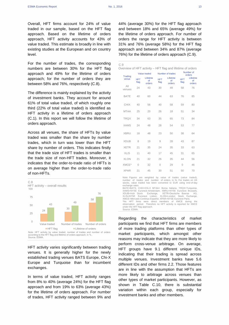
Overall, HFT firms account for 24% of value
traded in our sample, based on the HFT flag
approach. Based on the lifetime of orders
approach, HFT activity accounts for 43% of
value traded. This estimate is broadly in line with
existing studies at the European and on country
level.
For the number of trades, the corresponding
numbers are between 30% for the HFT flag
approach and 49% for the lifetime of orders
approach; for the number of orders they are
between 58% and 76%, respectively (C.8).
The difference is mainly explained by the activity
of investment banks. They account for around
61% of total value traded, of which roughly one
third (22% of total value traded) is identified as
HFT activity in a lifetime of orders approach
(C.1). In this report we will follow the lifetime of
orders approach.
Across all venues, the share of HFTs by value
traded was smaller than the share by number
trades, which in turn was lower than the HFT
share by number of orders. This indicates firstly
that the trade size of HFT trades is smaller than
the trade size of non-HFT trades. Moreover, it
indicates that the order-to-trade ratio of HFTs is
on average higher than the order-to-trade ratio
of non-HFTs.
C.8 HFT activity – overall results
HFT activity varies significantly between trading
venues. It is generally higher for the newly
established trading venues BATS Europe, Chi-X
Europe and Turquoise than for incumbent
exchanges.
In terms of value traded, HFT activity ranges
from 8% to 40% (average 24%) for the HFT flag
approach and from 19% to 63% (average 43%)
for the lifetime of orders approach. For number
of trades, HFT activity ranged between 9% and
44% (average 30%) for the HFT flag approach
and between 18% and 65% (average 49%) for
the lifetime of orders approach. For number of
orders the range for HFT activity is between
31% and 76% (average 58%) for the HFT flag
approach and between 34% and 87% (average
76%) for the lifetime of orders approach (C.9).
C.9 Overview of HFT activity – HFT flag and lifetime of orders
Trading venue
Value traded Number of trades Number of
orders
HFT flag
Lifetime of
orders
HFT flag
Lifetime of
orders
HFT flag
Lifetime of
orders
All venues
24 43 30 49 58 76
BATE 40 60 44 63 76 85
CHIX 40 56 40 58 59 80
MTAA 25 20 26 18 51 34
TRQX 34 63 35 65 73 84
XAMS 24 48 28 54 53 77
XBRU 18 48 23 50 38 64
XDUB 8 19 9 28 43 87
XETR 21 35 24 35 33 63
XLIS 11 40 17 45 31 65
XLON 21 32 26 35 44 56
XMCE* 0 32 0 29 0 46
XPAR 21 45 30 51 50 70
Note: Figures are weighted by value of trades (value traded), number of trades and number of orders, in %. For trades on UK stocks, value traded has been converted to EUR using end-of-day exchange rates. BATE=BATS, CHIX=Chi-X MTAA= Borsa Italiana, TRQX=Turquoise, XAMS=NYSE Euronext Amsterdam, XBRU=NYSE Euronext Brussels, XDUB=Irish Stock Exchange, XETR=Deutsche Boerse AG, XLIS=NYSE Euronext Lisbon, XLON=London Stock Exchange, XMCE=Mercado Continuo Español, XPAR=NYSE Euronext Paris. *No HFT firms were direct members of XMCE during the observation period. Therefore no HFT activity is reported for XMCE under the HFT flag approach. Source: ESMA.
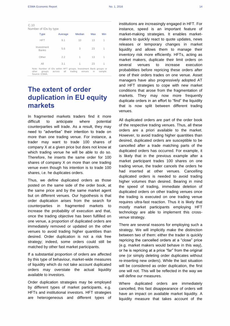
Regarding the characteristics of market
participants we find that HFT firms are members
of more trading platforms than other types of
market participants, which amongst other
reasons may indicate that they are more likely to
perform cross-venue arbitrage. On average,
HFT groups have 9.1 different unique IDs,
indicating that their trading is spread across
multiple venues. Investment banks have 5.6
different IDs and other firms 2.2. Those features
are in line with the assumption that HFTs are
more likely to arbitrage across venues than
other types of market participants. However, as
shown in Table C.10, there is substantial
variation within each group, especially for
investment banks and other members.
2430
58
4349
76
0
25
50
75
100
Value traded Number of trades Number of orders
HFT flag Lifetime of orders
Note: HFT activity by value traded, number of trades and number of ordersaccording to the HFT flag and lifetime of orders approach, in %..Source: ESMA.
ESMA Economic Report No. 1, 2016 14
C.10 Number of IDs by type
Type Average Median Max Min
HFT 9.1 10 13 1
Investment Banks
5.6 3 23 1
Other 2.2 1 13 1
All 3.1 1 23 1
Note: Number of IDs within HFT groups, Investment Bank groups or other groups across all trading venues in sample. Source: ESMA.
The extent of order duplication in EU equity markets
In fragmented markets traders find it more
difficult to anticipate where potential
counterparties will trade. As a result, they may
need to “advertise” their intention to trade on
more than one trading venue. For instance, a
trader may want to trade 100 shares of
company X at a given price but does not know at
which trading venue he will be able to do so.
Therefore, he inserts the same order for 100
shares of company X on more than one trading
venue even though his intention is to trade 100
shares, i.e. he duplicates orders.
Thus, we define duplicated orders as those
posted on the same side of the order book, at
the same price and by the same market agent
but on different venues. Our hypothesis is that
order duplication arises from the search for
counterparties in fragmented markets to
increase the probability of execution and that,
once the trading objective has been fulfilled on
one venue, a proportion of duplicated orders are
immediately removed or updated on the other
venues to avoid trading higher quantities than
desired. Order duplication is not a risk free
strategy; indeed, some orders could still be
matched by other fast market participants.
If a substantial proportion of orders are affected
by this type of behaviour, market-wide measures
of liquidity which do not take account duplicated
orders may overstate the actual liquidity
available to investors.
Order duplication strategies may be employed
by different types of market participants, e.g.
HFTs and institutional investors. HFT strategies
are heterogeneous and different types of
institutions are increasingly engaged in HFT. For
instance, speed is an important feature of
market-making strategies. It enables market-
makers to quickly react to quote updates, news
releases or temporary changes in market
liquidity and allows them to manage their
inventory risk more efficiently. HFTs, acting as
market makers, duplicate their limit orders on
several venues to increase execution
probabilities before repricing these orders after
one of their orders trades on one venue. Asset
managers have also progressively adopted AT
and HFT strategies to cope with new market
conditions that arose from the fragmentation of
markets. They may now more frequently
duplicate orders in an effort to “find” the liquidity
that is now split between different trading
venues.
All duplicated orders are part of the order book
of the respective trading venues. Thus, all these
orders are a priori available to the market.
However, to avoid trading higher quantities than
desired, duplicated orders are susceptible to be
cancelled after a trade matching parts of the
duplicated orders has occurred. For example, it
is likely that in the previous example after a
market participant trades 100 shares on one
trading venue, the trader cancels the orders he
had inserted at other venues. Cancelling
duplicated orders is needed to avoid trading
higher volumes than desired. Bearing in mind
the speed of trading, immediate deletion of
duplicated orders on other trading venues once
the trading is executed on one trading venue
requires ultra-fast reaction. Thus it is likely that
mostly market participants employing HFT
technology are able to implement this cross-
venue strategy.
There are several reasons for employing such a
strategy. We will implicitly make the distinction
between two of them: either the trader is quickly
repricing the cancelled orders at a “close” price
(e.g. market makers would behave in this way),
or he is repricing at a price “far” from the original
one (or simply deleting order duplicates without
re-inserting new orders). While the last situation
will be considered as order duplication, the first
one will not. This will be reflected in the way we
will define our measures.
Where duplicated orders are immediately
cancelled, this fast disappearance of orders will
have an impact on available market liquidity. A
liquidity measure that takes account of the

ESMA Economic Report No. 1, 2016 15
existence and the extent of order duplication
should therefore be more accurate than a gross
measure of liquidity that does not control for
order duplication.
Therefore, we introduce the concepts of gross
and net liquidity. Gross liquidity is computed as
the aggregated volume of displayed orders in
multiple markets for each market participant. Net
liquidity is calculated subtracting duplicated
orders from gross liquidity. Net liquidity is a more
genuine representation of the orders available in
the market but it is not observable by market
participants.
By aggregating across market participants we
are able to obtain a market-wide measure of
gross liquidity (which market participants can
observe) and a market-wide measure of net
liquidity (without duplicated orders and
unobservable by market participants).
To compute the net liquidity measure, we need
to define and compute duplicated orders for
each snapshot of the order book. Order book
snapshots are taken each 10 milliseconds in our
sample period.25 Basis for the calculation is the
mid-price, i.e. the average of the best bid and
ask prices across venues.
For all market participants, we calculate the
aggregated volume of displayed orders across
all venues within ± 0.5% of each mid-price.26 We
then aggregate across all market participants to
obtain the gross liquidity measure for this order
book snapshot. Then, we define net orders as
the largest order of a market participant on a
single venue within ± 0.5% of each mid-price.
Again, we aggregate across all market
participants to obtain our net liquidity measure.
25 As we are working with cross-venue order data, clock
synchronisation is an issue. The longest time interval of timestamps provided by trading venues to us is 3ms. By using orderbook snapshots at 10ms intervals we reduce the clock synchronisation bias, i.e. that orders are incorrectly included in an orderbook snapshot due to clock synchronisation issues.
26 The +/-0.5% spread is applied to all the stocks of the sample, without considering their specific liquidity and may be considered large for liquid stocks. We apply a common spread to all the stocks of the sample because it increases computing feasibility and we do not introduce a bias deriving from using a liquidity-based spread adjusted per stock to compute liquidity measures. Choosing a relatively large common spread avoids the issue of not capturing any orders in situations where the top of the order book would be outside the spread. On the other hand, a relatively large common spread will probably lead to the underestimation of order duplication – as duplication is more prevalent for narrower spreads.
The net liquidity measure is based on the
assumption that a trader pursuing a duplicated
orders strategy will at most execute the biggest
outstanding quantity for each stock within ±
0.5% of mid-price.
Finally, by construction, we define the duplicated
orders variable as the difference between gross
liquidity and net liquidity. Box 1 provides a
simple example of the order duplication metrics.
Order duplication metrics Box 1 Gross and net liquidity measures are calculated as follows for Agent 1:
gross liquidity is the aggregated volume of orders at a price of 10.00 across all venues: 500+300+200=1000
net liquidity is the largest of these orders: 500
duplicated orders: gross liquidity – net liquidity = 1,000 – 500 = 500
Similarly the gross liquidity for agent 2 is 300 shares; net liquidity is 150 shares, which implies duplicated orders of 150 shares. On a market wide basis, we compute the order duplication metrics as the sum of gross and net liquidity measures of all market participants, here agents 1 and 2:
gross liquidity: 1,000 + 300 = 1,300
net liquidity: 500 + 150 = 650
duplicated orders: gross liquidity – net liquidity = 1,300 – 650 = 650
Price Venue
1 Venue
2 Venue
3 Gross
Liquidity Net
Liquidity
Agent 1
10.00 500 300 200 1000 500
Agent 2
10.00 100 150 50 300 150
Total 600 450 250 1300 650
These metrics are computed for all stocks in our
sample at 10-millisecond intervals throughout
our sample period. We also consider separately
the two sides of the trading book (bid side and
ask side).
For instance, for a given stock i a given day 𝐷
and for the bid side of the order book, the gross
liquidity, net liquidity and duplicated orders
measures are computed the following way:
𝐺𝑟𝑜𝑠𝑠𝑖,𝐷,𝐵𝐼𝐷 =1
𝑁∑ ∑ ∑ 𝑄𝑣
𝑣 ∈ 𝛺𝑝𝑝 ∈ 𝛺𝑡
𝑁
𝑡=1
𝑁𝑒𝑡𝑖,𝐷,𝐵𝐼𝐷 =1
𝑁∑ ∑ max
𝑣 ∈ 𝛺𝑝
𝑄𝑣
𝑝 ∈ 𝛺𝑡
𝑁
𝑡=1
𝐷𝑢𝑝𝑙𝑖𝑐𝑎𝑡𝑒𝑑𝑆,𝐷,𝐵𝐼𝐷 = 𝐺𝑟𝑜𝑠𝑠𝑆,𝐷,𝐵𝐼𝐷 − 𝑁𝑒𝑡𝑆,𝐷,𝐵𝐼𝐷
Where:
— 𝑁 is the number of observations
— Ω𝑡 is the vector of prices available within ±
0.5% of the mid-price at observation time 𝑡27
27 At observation time t, for a given trader and for each
price we compute gross liquidity and net liquidity for all his orders at +/-0.5%.

ESMA Economic Report No. 1, 2016 16
— Ω𝑝 is the vector of trading venues for which
there exists an order at price p at
observation time 𝑡
— 𝑄𝑣 is the aggregated volume of displayed
orders available on venue 𝑣, at price 𝑝 and
at observation time 𝑡
To obtain the overall results, we take the
averages of the values calculated for each
existing combination of stock and day.
We analyse our sample differentiating between
HFTs and non-HFTs. As mentioned in the
previous section, in this report we identify HFTs
following the lifetime of orders approach. In our
sample, HFT activity, measured with this
approach, accounts for 43% of the value traded,
49% of the number of trades and 76% of the
number of orders.28
In the overall sample, duplicated orders account
for around 20% of all orders and are broadly
homogeneous on both sides of the order
book. 29 The extent of duplicated orders varies
significantly between HFT firms and non-HFT
firms; for HFTs duplicated orders account for
around 34% of all their orders compared to 12%
for non-HFTs (C.11).
C.11 Duplicated orders – HFT vs non-HFT across sample
The extent of order duplication also depends on
stock characteristics. We therefore look at order
duplication by market capitalisation, price
volatility and trading fragmentation of the shares
in our sample. In all of these cases we also
differentiate between the extent of order
duplication for HFTs and non-HFTs.
When we take into account the different
categories of market capitalisation (large caps,
mid caps and small caps) duplicated orders
28 See ESMA (2014) for more details on different HFT
identification approaches.
29 The amount of duplicated orders is calculated as the average of the stock daily averages of all 10ms intervals.
seem to be more relevant for large caps (23%
compared to 11% for small caps), consistent
with the evidence showing that HFTs are more
active in this market segment.30 As expected, we
do not find any significant difference between
the buy side and the sell side of the book.
Across different categories of market
capitalisation, HFTs consistently display a higher
percentage of duplicated orders than non-HFTs
(C.12).
C.12 Duplicated orders – by market capitalisation
The extent of order duplication is lower for the
shares in our sample with higher price volatility
during our sample period (16% for high-volatility
stocks compared to 22% for low-volatility
stocks). Using duplicated orders implies the risk
of trading more shares than desired if order
duplicates are matched on more than one
trading venue. Observing less duplicated orders
when uncertainty is higher is consistent with
reducing this risk. Duplicated orders are
consistently more relevant for HFTs than for
non-HFTs when different levels of price volatility
are taken into account. Moreover, we observe
that the extent of order duplication for HFTs
varies with volatility; there are only small
changes in the extent of order duplication for
non-HFTs with volatility levels (C.13).31
30 See e.g. Brogaard et al (2013) and ESMA (2014).
31 Overall levels of price volatility were low in our sample period of May 2013 (see C.7). Hence, our results regarding order duplication and volatility may be substantially different in periods with high market-wide volatility.
2034
12
8066
88
0
25
50
75
100
Overall HFT Non-HFT
Non-duplicated orders Duplicated orders
Note: Duplicated orders, in %, for HFTs, non-HFTs and overall.Source: ESMA.
34 3632
1412 13
9 9
2022
1512
0
10
20
30
40
Full sample Large caps Mid caps Small caps
HFT Non-HFT Overall
Note: Proportion of duplicated orders by market capitalisation, displayed forHFTs, non-HFTs and total. In %.Sources: Thomson Reuters Datastream, ESMA.

ESMA Economic Report No. 1, 2016 17
C.13 Duplicated orders – by price volatility
As expected (see e.g. Van Kervel, 2015)
fragmentation is positively correlated with order
duplication. In markets characterised by high
fragmentation, duplicated orders range from
14% for non-HFTs to 36% for HFTs. When
fragmentation is low the proportion of duplicated
orders is 7% and 29% respectively (C.14).
C.14 Duplicated orders – by trading fragmentation
In the next sections we analyse in more detail
how duplicated orders are used and whether our
net liquidity measure better reflects available
liquidity in fragmented markets compared to a
gross liquidity measure.
— First we analyse the behaviour of trade
participants, especially to which extent they
use duplicated orders and cancel them after
a trade.
— Second, we carry out descriptive and
econometric analyses to look at the different
reaction of two market-wide measures of
liquidity after trades: gross liquidity,
computed for each market participant as the
aggregated volume of displayed orders in
multiple markets, and net liquidity, computed
subtracting duplicated orders from gross
orders. A steeper decline of the gross
liquidity measure after trades compared to
the net liquidity measure is an indication that
in some cases duplicated orders are indeed
immediately cancelled after trades and thus
are de facto not available to the market. Net
liquidity would then provide a more accurate
picture of available liquidity in fragmented
markets.
The behaviour of trade participants
In this section we analyse the behaviour of
traders who provided liquidity, i.e. have been on
the passive side of a trade. We distinguish
between four types of behaviour:32
a) Use of duplicated orders and immediate
cancellation of non-matched order
duplicates or update of order duplicates at
more than ±0.5% of the trade price;
b) Use of duplicated orders and no cancellation
of order duplicates;
c) Use of duplicated orders and update of
order duplicates at less than ±0.5% of the
trade price;
d) No use of duplicated orders.
In case a) order duplicates are de facto not
available to the market, as they are either
quickly withdrawn or updated at a price which is
far away from the last trade price and thus far
from the top of the order book. Overall we find
that in in 24% of trades the trader immediately
cancels his unmatched duplicated orders or
updates them at a price far from the trade price.
In cases b) and c) order duplicates are available
to the market. For 15% of the trades traders use
duplicated orders and do not cancel them after a
trade (case b). For 9% of the trades traders use
duplicated orders and update them at a price
close to the trade price (case c). For 52% of the
trades the trader makes no use of order
duplication (case d; C.15).
As shown in C.15 to C.18 results vary
depending on trader and stock characteristics.
32 We analyse the first reaction of the trader within 500ms
of the trade.
34
28
35 36
12 11 12 12
2017
21 21
0
10
20
30
40
Full sample High volatility Mediumvolatility
Low volatility
HFT Non-HFT Overall
Note: Proportion of duplicated orders by price volatility for the sample stocks,displayed for HFTs, non-HFTs and total. In %.Source: ESMA.
34 36
30 29
1214
117
2023
18
13
0
10
20
30
40
Full sample Highfragmentation
Mediumfragmentation
Lowfragmentation
HFT Non-HFT Overall
Note: Proportion of duplicated orders by trading fragmentation for the samplestocks, displayed for HFTs, non-HFTs and total. In %.Source: ESMA

ESMA Economic Report No. 1, 2016 18
C.15 Behaviour of trader after trade event
Order duplication is more common for large cap
shares with traders using order duplication in
53% of trades, while it tends to be less frequent
in case of mid cap and small cap stocks (39%
and 20% respectively). The same pattern is
observed for the traders immediately deleting
their orders after the trade is executed; we
observe this behaviour for 27% of trades in large
cap stocks, 18% for mid cap and 9% for small
cap stocks. Similarly, order duplication and
immediate update of new orders close to the
trade price is observed more frequently for large
cap stocks (11%) than for mid cap and small cap
stocks (7% and 3% respectively; C.16).
C.16 Behaviour of trader after trade event – by market capitalisation
The analysis of order duplication strategies for
different levels of market fragmentation confirms
our previous results. We find that duplicated
orders are present in 59% of trades when
market fragmentation is high, but only in 24% of
trades when market fragmentation is low. The
difference is even larger when the order
duplication and cancellation behaviour is
considered; this strategy is performed by 31% of
traders in stocks where trading is highly
fragmented while in a low fragmentation
environment it is limited to 10% of trades (C.17).
C.17 Behaviour of trader after trade event – by fragmentation of trading
Finally, we do not observe different behaviour
with respect to order duplication strategies and
the size of the trade (C.18).
C.18 Behaviour of trader after trade event – by trade size
Impact of trading on gross and net liquidity
Descriptive analysis
We have identified a significant proportion of
duplicated orders in our sample. If those
duplicated orders are immediately cancelled
after a trade has taken place, this result points at
a risk of systematic overestimation of liquidity in
fragmented equity markets. In the previous
chapter we established that for 24% of trades
duplicated orders are involved on the passive
side of the trade and immediately cancelled after
the trade.
An alternative way to look at this question is to
analyse the decrease in gross and net liquidity
measures after a trade. We introduced the
concepts of gross and net liquidity earlier to
establish the extent of order duplication. If we
consistently observe a stronger decrease for the
gross liquidity measure compared to the net
24 28 20
913
6
1515
15
52 4460
0
25
50
75
100
Overall HFT Non-HFTs
No duplication Duplication + No cancellationDuplication + Update Duplication + Cancellation
Note: Trades by order duplication strategy and action within 500ms after trade fortraders on the passive side of the trade. 1) No duplicated orders. 2) Duplicatedorders and cancellation of order duplicates. 3) Duplicated orders and update oforder duplicates 4) Duplicated orders and no action. For overall sample, HFTsand non-HFTs. In %.Source: ESMA.
24 27 18 9
9 117
3
15 15
15
9
52 4761
80
0
25
50
75
100
Overall Large caps Mid caps Small capsNo duplication Duplication + No cancellationDuplication + Update Duplication + Cancellation
Note: Trades by order duplication strategy and action within 500ms after trade fortraders on the passive side of the trade. 1) No duplicated orders. 2) Duplicatedorders and cancellation of order duplicates. 3) Duplicated orders and update oforder duplicates 4) Duplicated orders and no action. For overall sample, largecap, mid cap and small cap stocks. In %.Sources: Thomson Reuters Datastream, ESMA.
24 3117 10
912
84
1517
1311
52 4163
76
0
25
50
75
100
Overall Highfragmentation
Mediumfragmentation
Lowfragmentation
No duplication Duplication + No cancellationDuplication + Update Duplication + Cancellation
Note: Trades by order duplication strategy and action within 500ms after trade fortraders on the passive side of the trade. 1) No duplicated orders. 2) Duplicatedorders and cancellation of order duplicates. 3) Duplicated orders and update oforder duplicates 4) Duplicated orders and no action. For overall sample, stockswith high, medium and low trading fragmentation. In %.Source: ESMA.
24 25 24 22
9 11 9 7
15 11 15 18
52 52 51 53
0
25
50
75
100
Overall Large trades Medium trades Small tradesNo duplication Duplication + No cancellationDuplication + Update Duplication + Cancellation
Note: Trades by order duplication strategy and action within 500ms after trade fortraders on the passive side of the trade. 1) No duplicated orders. 2) Duplicatedorders and cancellation of order duplicates. 3) Duplicated orders and update oforder duplicates 4) Duplicated orders and no action. For overall sample, large,medium and small trades in sample. Large, medium, small trades represent thefirst, second and third tercile of trades in our sample by trade size. In %.Source: ESMA.

ESMA Economic Report No. 1, 2016 19
liquidity measure after a trade, this indicates that
duplicated orders are indeed often cancelled
directly after trades. Taking them into account
when measuring liquidity in fragmented markets
would thus overestimate available liquidity and
the concept of net liquidity would be a more
accurate measure of available liquidity in
fragmented markets.
In this section we look at the impact of trades on
gross and net liquidity measures. We run the
empirical analysis on 95 stocks33 from 9
countries for 23 trading days in May 2013. We
consider all trades occurring on the trading
venues included in our sample between 9:15
and 17:15. We exclude trading occurring in the
first and last 15 minutes of the day to avoid
auction periods. We look at the reaction of gross
and net liquidity in specific non-overlapping
windows, 100ms and 500ms after each trade.34
The 100ms and 500ms samples do not intersect
each other, the 500ms sample contains all the
trades for which there has not been any trade in
the following 500ms. Therefore, the 100ms
sample contains all the trade for which there has
been a trade between 100ms and 500ms after a
trade event3536.
We analyse the change of gross and net liquidity
divided by the size of the respective trade after
each trade. We are interested in understanding
33 Five stocks were excluded due to an insufficient number
of trades and insufficient liquidity (1 for Ireland, 1 for Portugal, 1 for France, 1 for the United Kingdom and 1 for the Netherlands).
34 Windows are non-overlapping and contain only a single trade.
35 The 100ms sample generally includes trades for more liquid, mostly large cap stocks. Trade events for these stocks are absorbed more quickly in the order book. Choosing a longer time window will decrease the sample of available trades for liquid stocks, as these are traded very frequently and thus longer time windows will very often include more than one trade, implying that these trades have to be removed from our sample. The 500ms includes a larger proportion of mid and small cap stocks, which are less liquid. For less liquid stocks it takes longer for a trade event to be absorbed in the order book, hence the need for a longer time window. As robustness check we also tested a 1000ms window with similar results compared to the 500ms window.
36 It is more likely that subsequent trades take place within the 100ms or 500ms when the initial trade had a low impact on market liquidity and the bid-ask spread is still attractive to market participants. In that sense we are aware that our non-overlapping samples may be affected by a bias, as higher impact trades are more likely represented in our samples. However, the bias affects both the gross and net measures of liquidity in a similar way. As the variable we are interested in is the difference in reaction between the gross and net liquidity measures, we consider that our analysis still provides valuable insights.
how strongly the order book reacts on average
to a given trade size.37 A priori, we expect
stronger reduction of both gross and net liquidity
in the 100ms window. The 100ms is likely to
capture the trades of more liquid stocks, where
orders are updated more frequently, which in
turn would lead to a stronger reduction of the
gross and net liquidity measures.
For each stock, the cumulated impact of a trade
occurring at 𝑡0 on the buy-side of the order book
for the gross liquidity at t = 𝑇 is computed as
follows:
∑ ∆𝐿𝑖𝑞𝑢𝑖𝑑𝑖𝑡𝑦(𝑏𝑢𝑦)𝑖𝑡𝑇𝑡=𝑡0
/ 𝑇𝑟𝑎𝑑𝑒_𝑆𝑖𝑧𝑒𝑖𝑡0
Where ∆𝐿𝑖𝑞𝑢𝑖𝑑𝑖𝑡𝑦(𝑏𝑢𝑦)𝑖𝑡 is the difference
between the gross liquidity available at time t
and at time t-1 on the buy side of the order book
for stock i.38
To reduce the impact of outliers, we remove the
top and bottom 1% of observations. We then
compute a simple average to build the gross and
net liquidity curves for the buy side of the order
book. Calculations for sell-side gross liquidity
and buy-side and sell-side net liquidity are
carried out in a similar way.
Our results show that across different samples
the reduction in gross liquidity is always higher
than the reduction in net liquidity for both 100ms
and 500ms windows. C.19 shows the decrease
of the gross and net liquidity measures (divided
by the trade size) in response to a trade for the
100ms window on the buy side of the order
book. Gross and net liquidity are computed in
discrete data points corresponding to the end of
10ms periods.39 We have order book snapshots
at 10ms intervals. This means that the trades
take place at some point in the interval -10ms to
0ms. The biggest decrease of available liquidity
occurs in the first 10ms after the trade; the size
37 This measure is similar to the one used by Van Kervel
(2015). Changes in liquidity closely related to trade events do not suffer scale sensitivity. We carried out robustness checks to ensure the gross and net liquidity measures are not differently affected by trade sizes.
38 Similarly, for each stock, the cumulated impact of a trade occurring at t=0 on the sell-side of the order book for the gross liquidity at t=T is computed as ∑ ∆𝐿𝑖𝑞𝑢𝑖𝑑𝑖𝑡𝑦(𝑠𝑒𝑙𝑙)𝑖𝑡
𝑇𝑡=𝑡0
/ 𝑇𝑟𝑎𝑑𝑒_𝑆𝑖𝑧𝑒𝑖𝑡0, where
∆Liquidity(sell)it is the difference between the gross liquidity available at time t and at time t-1 on the sell side of the order book for stock i.
39 As mentioned in the previous section the most detailed interval available for computing liquidity is 3ms, as for some of the reporting venues the timestamp was provided with such detail. We picked 10ms interval because it is easier to truncate timestamps to 10ms rather than to 3ms and we keep a reasonable precision.

ESMA Economic Report No. 1, 2016 20
of this reaction is depicted at 0ms on the x-axis
of graphs C.19 and C.20. Part of this reaction is
explained by the trade itself. However, as
described in previous section in 24% of trades
the trader immediately cancels his unmatched
duplicated orders or updates them at a price far
from the trade price, which explains the stronger
fall in the net liquidity measure.
C.19 Reaction of gross and net liquidity in the 100ms window – overall sample
Similar results are obtained when a larger time
window is considered. C.20 shows the reduction
of gross and net liquidity for the 500ms window
on the buy side of the order book. The liquidity
decrease for the 100ms window is always more
pronounced than for the 500ms window.
C.20 Reaction of gross and net liquidity in the 500 ms window – overall sample
The results remain robust when the sell side of
the order book is considered or when different
categories of market capitalisation, price
volatility and market fragmentation are taken into
account. In line with the empirical evidence on
the level of duplicated orders seen in the
descriptive statistics part, the strength of
reaction to trade by large caps, stocks with low
price volatility and high fragmentation is higher
compared to small caps, stocks with high price
volatility and low fragmentation. These results
are presented in Annex 240.
Time series analysis
The time-series analysis is inspired by Van
Kervel (2015): it tests the hypothesis that a trade
on one venue is followed by changes in the
order book liquidity for a stock on both the bid
and ask sides of all venues.
The dependent variable is
∆𝐿𝑖𝑞𝑢𝑖𝑑𝑖𝑡𝑦(𝑠)𝑖𝑡 = 𝐿𝑖𝑞𝑢𝑖𝑑𝑖𝑡𝑦(𝑠)𝑖𝑡 − 𝐿𝑖𝑞𝑢𝑖𝑑𝑖𝑡𝑦(𝑠)𝑖𝑡−1
Where s indicates the trade side, 𝑠 ∈ {𝑏𝑢𝑦, 𝑠𝑒𝑙𝑙}.
Changes in Liquidity (buy) and Liquidity (sell)
reflect changes in liquidity offered at prices in
the interval {midpricet-1 ± 0.5%}. These changes
arise from limit order book activity (placements,
cancellations and executions of limit orders).
The models regresses the change in Liquidity
(buy) or Liquidity (sell) on the contemporaneous
and lagged buy and sell trading volumes of all
the trading venues in the database. The model
contains lags up to 1000ms to allow for sufficient
time for the market to incorporate the
information content of trades.
The time-series approach enables us to refine
our analysis of duplicated order strategies in two
ways. In contrast with the previous descriptive
analysis, in the time-series analysis there is no
need to remove from the sample close-in-time
trades, preventing the possibility of sampling
bias. As in the previous approach, periods close
to the opening and closing of the trading are
excluded.
We estimate coefficients for five groups of
lagged variables and assume that the
coefficients are constant within each group. This
is obtained by adding in the regression five
average lagged trading volumes of the following
intervals of milliseconds L1=[0,10], L2=[10,40],
L3=[40,100], L4=[100,200], L5=[200,1000].
40 The difference between the reactions of the gross and
net liquidity is more interesting than the absolute values of the decrease in the measures: The 100ms window, by construction, is capturing trades in more liquid stocks. Therefore, the overall reaction is likely to be stronger than for a less liquid stock. When defining the windows, we checked for trades occurring in the following 100 or 500ms but not before. Some of the trades in our sample are at the end of a series of trades. In these cases the reaction observed after the trade, i.e. the decrease in the gross and net liquidity measures will be higher than the results for trades which are not at the end of a series of trade.
-4
-3
-2
-1
0
-10 0 10 20 30 40 50 60 70 80 90 100
Gross Buy Net BuyNote: Y-axis depicts the variation in time of available liquidity levels, Gross andNet measures, divided by the size of each trade. Given data constraints,available liquidity is only computed in equally-spaced and discrete points in time(each 10 ms). The X-axis represents time in ms; the trade takes place in the-10ms and the 0ms interval.Source: ESMA.
-4
-3
-2
-1
0
-10 30 70 110 150 190 230 270 310 350 390 430 470 500
Gross Buy Net BuyNote: Y-axis depicts the variation in time of available liquidity levels, Gross andNet measures, divided by the size of each trade. Given data constraints,available liquidity is only computed in equally-spaced and discrete points in time(each 10 ms). The X-axis represents time in ms; the trade takes place in the-10ms and the 0ms interval.Source: ESMA.
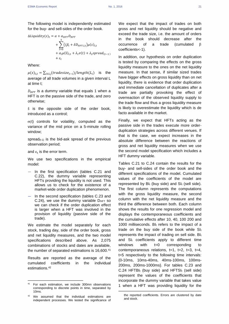
ESMA Economic Report No. 1, 2016 21
The following model is independently estimated
for the buy- and sell-sides of the order book.
∆𝐿𝑖𝑞𝑢𝑖𝑑𝑖𝑡𝑦(𝑠)𝑡 = 𝛼 + 𝛼𝐻𝐹𝑇𝐷𝐻𝐹𝑇
+ ∑((𝛽𝑙 + 𝛿𝐷𝐻𝐹𝑇,𝑙,𝑡)𝜇(𝑠)𝑙,𝑡
5
𝑙=0
+ 𝛼𝑙𝜇(š)𝑙,𝑡 + 𝜆1𝜎(𝑡) + 𝜆2𝑠𝑝𝑟𝑒𝑎𝑑(𝑡−1 )
+ 휀𝑡
Where:
𝜇(𝑠)𝑙,𝑡 = ∑ (𝑡𝑟𝑎𝑑𝑒𝑠𝑖𝑧𝑒𝑡−𝑖)/𝑙𝑒𝑛𝑔𝑡ℎ(𝐿𝑙)𝑖∈𝐿𝑙 is the
average of all trade volumes in a given interval L
at time t;
𝐷𝐻𝐹𝑇 is a dummy variable that equals 1 when a
HFT is on the passive side of the trade, and zero
otherwise;
š is the opposite side of the order book,
introduced as a control;
t) controls for volatility, computed as the
variance of the mid price on a 5-minute rolling
window;
spread(t-1) is the bid-ask spread of the previous
observation period;
and εt is the error term.
We use two specifications in the empirical
model:
— In the first specification (tables C.21 and C.22), the dummy variable representing HFTs providing the liquidity is not used. This allows us to check for the existence of a market-wide order duplication phenomenon.
— In the second specification (tables C.23 and C.24), we use the dummy variable DHFT so we can check if the order duplication effect is larger when a HFT was involved in the provision of liquidity (passive side of the trade).
We estimate the model separately for each
stock, trading day, side of the order book, gross
and net liquidity measures, and the two model
specifications described above. As 2,075
combinations of stocks and dates are available,
the number of separated estimations is 16,600.41
Results are reported as the average of the
cumulated coefficients in the individual
estimations.42
41 For each estimation, we include 300mn observations
corresponding to discrete points in time, separated by 10ms.
42 We assumed that the individual estimations are independent processes. We tested the significance of
We expect that the impact of trades on both
gross and net liquidity should be negative and
exceed the trade size, i.e. the amount of orders
in the book should decrease after the
occurrence of a trade (cumulated
coefficients<-1).
In addition, our hypothesis on order duplication
is tested by comparing the effects on the gross
liquidity measure to the ones on the net liquidity
measure. In that sense, if similar sized trades
have bigger effects on gross liquidity than on net
liquidity, there is evidence that order duplication
and immediate cancellation of duplicates after a
trade are partially provoking the effect of
overreaction of the observed liquidity supply to
the trade flow and thus a gross liquidity measure
is likely to overestimate the liquidity which is de
facto available in the market.
Finally, we expect that HFTs acting as the
passive side in the trades execute more order-
duplication strategies across different venues. If
that is the case, we expect increases in the
absolute difference between the reactions of
gross and net liquidity measures when we use
the second model specification which includes a
HFT dummy variable.
Tables C.21 to C.24 contain the results for the
buy- and sell-sides of the order book and the
different specifications of the model. Cumulated
values of the coefficients of the model are
represented by BIt (buy side) and SIt (sell side).
The first column represents the computations
with the gross liquidity measure, the second
column with the net liquidity measure and the
third the difference between both. Each column
shows the results for one regression model and
displays the contemporaneous coefficients and
the cumulative effects after 10, 40, 100 200 and
1000 milliseconds. BIt refers to the impact of a
trade on the buy side of the book while SIt
represents the impact of trading on sell side. BIt
and SIt coefficients apply to different time
windows with t=0 corresponding to
contemporaneous relations, t=1, t=2, t=3, t=4,
t=5 respectively to the following time intervals:
{0-10ms, 10ms-40ms, 40ms-100ms, 100ms-
200ms, 200ms-1000ms}. For tables C.23 and
C.24 HFTBIt (buy side) and HFTSIt (sell side)
represent the values of the coefficients that
incorporate the dummy variable that takes value
1 when a HFT was providing liquidity for the
the reported coefficients. Errors are clustered by date and stock.
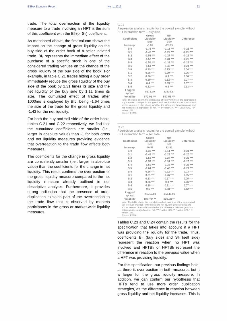
ESMA Economic Report No. 1, 2016 22
trade. The total overreaction of the liquidity
measure to a trade involving an HFT is the sum
of this coefficient with the BIt (or SIt) coefficient.
As mentioned above, the first column shows the
impact on the change of gross liquidity on the
buy side of the order book of a seller initiated
trade. BI0 represents the immediate effect of the
purchase of a specific stock in one of the
considered trading venues on the change of the
gross liquidity of the buy side of the book. For
example, in table C.21 trades hitting a buy order
immediately reduce the gross liquidity of the buy
side of the book by 1.31 times its size and the
net liquidity of the buy side by 1.11 times its
size. The cumulated effect of trades after
1000ms is displayed by BI5, being -1.64 times
the size of the trade for the gross liquidity and
-1.43 for the net liquidity.
For both the buy and sell side of the order book,
tables C.21 and C.22 respectively, we find that
the cumulated coefficients are smaller (i.e.,
larger in absolute value) than -1 for both gross
and net liquidity measures providing evidence
that overreaction to the trade flow affects both
measures.
The coefficients for the change in gross liquidity
are consistently smaller (i.e., larger in absolute
value) than the coefficients for the change in net
liquidity. This result confirms the overreaction of
the gross liquidity measure compared to the net
liquidity measure already outlined in our
descriptive analysis. Furthermore, it provides
strong indication that the presence of order
duplication explains part of the overreaction to
the trade flow that is observed by markets
participants in the gross or market-wide liquidity
measures.
C.21 Regression analysis results for the overall sample without HFT interaction term – buy side
Coefficient Gross
Liquidity Buy
Net Liquidity
Buy Difference
Intercept -8.81 -25.05
BI0 -1.31 *** -1.11 *** -0.21 ***
BI1 -1.47 *** -1.22 *** -0.25 ***
BI2 -1.53 *** -1.27 *** -0.26 ***
BI3 -1.57 *** -1.31 *** -0.26 ***
BI4 -1.59 *** -1.33 *** -0.26 ***
BI5 -1.64 *** -1.43 *** -0.21 ***
SI0 0.29 *** 0.25 *** 0.04 ***
SI1 0.35 *** 0.29 *** 0.06 ***
SI2 0.36 *** 0.3 *** 0.06 ***
SI3 0.39 *** 0.32 *** 0.07 ***
SI4 0.4 *** 0.33 *** 0.07 ***
SI5 0.52 *** 0.4 *** 0.13 ***
Lagged spread
8172.29 22825.87
Volatility 672.01 *** 547.56 ***
Note: The table shows the cumulative effect over time of the aggregated buy turnover changes in the gross and net liquidity across stocks and across venues. It also shows whether the difference between gross and net measures is significant or not. *** P-value<1%, ** P-value<5%, * P-value<10%. Source: ESMA.
C.22 Regression analysis results for the overall sample without HFT interaction term – sell side
Coefficient Gross
Liquidity Sell
Net Liquidity
Sell Difference
Intercept 40.51 12.81
SI0 -1.32 *** -1.11 *** -0.21 ***
SI1 -1.48 *** -1.23 *** -0.25 ***
SI2 -1.53 *** -1.27 *** -0.26 ***
SI3 -1.57 *** -1.31 *** -0.26 ***
SI4 -1.59 *** -1.33 *** -0.26 ***
SI5 -1.64 *** -1.43 *** -0.21 ***
BI0 0.26 *** 0.22 *** 0.03 ***
BI1 0.31 *** 0.26 *** 0.05 ***
BI2 0.33 *** 0.27 *** 0.05 ***
BI3 0.36 *** 0.3 *** 0.06 ***
BI4 0.38 *** 0.31 *** 0.07 ***
BI5 0.5 *** 0.38 *** 0.12 ***
Lagged spread
-41213.03 -15149.08
Volatility 1087.04 ** 820.28 ** Note: The table shows the cumulative effect over time of the aggregated sell turnover changes in the gross and net liquidity across stocks and across venues. It also shows whether the difference between gross and net measures is significant or not. *** P-value<1%, ** P-value<5%, * P-value<10%. Source: ESMA.
Tables C.23 and C.24 contain the results for the
specification that takes into account if a HFT
was providing the liquidity for the trade. Thus,
coefficients BIt (buy side) and SIt (sell side)
represent the reaction when no HFT was
involved and HFTBIt or HFTSIt represent the
difference in reaction to the previous value when
a HFT was providing liquidity.
For this specification, our previous findings hold,
as there is overreaction in both measures but it
is larger for the gross liquidity measure. In
addition, we can confirm our hypothesis that
HFTs tend to use more order duplication
strategies, as the difference in reaction between
gross liquidity and net liquidity increases. This is

ESMA Economic Report No. 1, 2016 23
reflected in the negative values for the difference
column for the coefficients HFTBIt (buy side)
and HFTSIt (sell side) in tables C.23 and C.24.
However, although the difference between
reactions of gross and net liquidity measures
increases when HFTs provide the liquidity for
the trade, the level of overreaction for both
measures is decreased. This is shown by the
positive values of the coefficients HFTBIt (buy
side) and HFTSIt (sell side) in the gross liquidity
and net liquidity columns of tables C.23 and
C.24. Even though these results are still in line
with our hypotheses, they warrant further
investigation regarding the reasons behind
them.
C.23 Regression analysis results for the overall sample with HFT interaction term – buy side
Coefficient Gross
Liquidity Buy
Net Liquidity
Buy Difference
HFT Intercept
-88.08 *** -71.79 ***
Intercept 5.36 -25.12
BI0 -1.41 *** -1.23 *** -0.18 ***
BI1 -1.58 *** -1.35 *** -0.23 ***
BI2 -1.64 *** -1.4 *** -0.24 ***
BI3 -1.69 *** -1.44 *** -0.24 ***
BI4 -1.72 *** -1.48 *** -0.24 ***
BI5 -1.74 *** -1.57 *** -0.18 ***
HFTBl0 0.11 *** 0.16 *** -0.05 ***
HFTBl1 0.11 *** 0.15 *** -0.04 ***
HFTBl2 0.11 *** 0.15 *** -0.04 ***
HFTBl3 0.11 *** 0.16 *** -0.05 ***
HFTBl4 0.11 *** 0.16 *** -0.05 ***
HFTBl5 0.2 *** 0.28 *** -0.08 **
SI0 0.29 *** 0.25 *** 0.04 ***
SI1 0.35 *** 0.29 *** 0.06 ***
SI2 0.37 *** 0.3 *** 0.06 ***
SI3 0.39 *** 0.33 *** 0.07 ***
SI4 0.4 *** 0.33 *** 0.07 ***
SI5 0.53 *** 0.41 *** 0.12 ***
Lagged spread
-4173.07 24376.39
Volatility 728.61 *** 584.53 *** Note: The table shows the cumulative effect over time of the aggregated buy turnover changes in the gross and net liquidity across stocks and across venues. It also shows whether the difference between gross and net measures is significant or not. *** P-value<1%, ** P-value<5%, * P-value<10%. Source: ESMA.
C.24 Regression analysis results for the overall sample with HFT interaction term – sell side
Coefficient Gross
Liquidity Sell
Net Liquidity
Sell Difference
HFT Intercept
-95.14 *** -77.11 ***
Intercept 43.75 14.34
SI0 -1.38 *** -1.21 *** -0.17 ***
SI1 -1.57 *** -1.36 *** -0.21 ***
SI2 -1.61 *** -1.39 *** -0.23 ***
SI3 -1.67 *** -1.44 *** -0.23 ***
SI4 -1.68 *** -1.46 *** -0.22 ***
SI5 -1.75 *** -1.58 *** -0.17 ***
HFTSl0 0.07 *** 0.12 *** -0.05 ***
HFTSl1 0.1 *** 0.15 *** -0.05 ***
HFTSl2 0.09 *** 0.14 *** -0.05 ***
HFTSl3 0.11 *** 0.16 *** -0.05 ***
HFTSl4 0.12 *** 0.18 *** -0.06 ***
HFTSl5 0.28 *** 0.32 *** -0.05 ***
BI0 0.26 *** 0.22 *** 0.03 ***
BI1 0.31 *** 0.26 *** 0.05 ***
BI2 0.33 *** 0.28 *** 0.05 ***
BI3 0.36 *** 0.3 *** 0.06 ***
BI4 0.39 *** 0.32 *** 0.07 ***
BI5 0.53 *** 0.4 *** 0.12 ***
Lagged spread
-42586.98 -15152.75
Volatility 1168.13 ** 876.39 ** Note: The table shows the cumulative effect over time of the aggregated sell turnover changes in the gross and net liquidity across stocks and across venues. It also shows whether the difference between gross and net measures is significant or not. *** P-value<1%, ** P-value<5%, * P-value<10%. Source: ESMA.
Conclusion
This report describes the results of our analysis
on order duplication and liquidity measurement
in fragmented EU equity markets.
This report is the second part of ESMA’s HFT
research. The starting point for both reports is
the change in the trading landscape of equity
markets over the last decade. The defining
features of this change are increased
competition between trading venues,
fragmentation of trading of the same financial
instruments across EU venues and the
increased use of fast and automated trading
technologies. In our first report we analysed the
extent of HFT activity across the EU in such an
environment using a novel identification method
for HFT activity. We found that HFT activity
represents between 24% and 43% of value
traded and between 58% and 76% of orders in
our sample. In this report we focus on liquidity
measurement where equity trading is
fragmented.
In an environment characterised by competition
between trading venues, traders do not always
know on which venue they will be able to trade.
They may “advertise” their intention to trade by
posting similar orders on more than one trading
venue at the same time (“duplicated orders”).

ESMA Economic Report No. 1, 2016 24
This, however, leads to the risk of trading more
shares than wanted. Therefore some traders
may immediately cancel unmatched duplicated
orders on other venues after one of their
duplicated orders has been filled.
Using the HFT identification method developed
in our first report, we find evidence for this
trading pattern. 20% of the orders in our sample
are duplicated orders and in 24% of trades the
trader immediately cancels unmatched
duplicated orders. We believe that duplication of
orders and immediate cancellation of duplicates
after a trade has become part of the strategy to
ensure execution in fragmented markets, e.g. for
market makers or where institutional investors
are searching for liquidity. However, we show
that taking duplicated orders into account when
measuring liquidity leads to overestimation of
available liquidity in fragmented markets.
The proportion of duplicated orders varies with
the type of traders, the market capitalisation of
the underlying stock and the fragmentation of
trading in a stock. As expected, duplicated
orders are more prevalent for HFTs (34% of
orders) than for non-HFTs (12% of orders). They
account for 22% of orders in large cap stocks
compared to 12% of orders in small cap stocks.
Also, fragmentation of trading is positively
correlated with order duplication. We find 13% of
duplicated orders for stocks with low trading
fragmentation and 23% for stocks with high
fragmentation.
Regarding the extent to which duplicated orders
are immediately cancelled after trades (and thus
subsequently are not available to the market),
we carry out a number of analyses. First, we find
that for 24% of all trades, the trader on the
passive side of the trade immediately cancels
order duplicates after the trade. This proportion
is higher for HFTs (28%), large cap stocks
(27%) and where trading is more fragmented
(31%). Second, we look at the different reaction
of two measures of liquidity: gross liquidity, the
aggregated volume of displayed orders across
multiple markets, and net liquidity, which
deducts duplicated orders from the gross
liquidity measure. We compare these two
measures to establish whether order duplication
should be taken into account when measuring
liquidity in fragmented markets. A stronger fall of
the gross liquidity measure after trades
compared to the net liquidity measure is an
additional indication that a proportion of
duplicated orders is indeed immediately
cancelled after trades and thus not available to
the market. Our descriptive and econometric
analyses confirm this hypothesis.
Both in our first HFT report and in this report we
use unique data collected by ESMA, covering a
sample of 100 stocks on 12 trading venues in
nine EU countries for May 2013. Our data allow
us to identify market participants’ actions across
different venues. Thus we are able to
complement the literature, as most of the HFT
studies published so far focus either on the US
or on a single country within Europe and few are
able to analyse the behaviour of market
participants across trading venues.
Previous studies have found evidence
supporting that fragmentation of trading
increases liquidity in equity markets. Our
analysis qualifies these results, as using data
that allow us to identify market participants’
actions across different venues, we find a
substantial extent of order duplication in
fragmented markets. It is important to state that
unless they are successfully cancelled,
duplicated orders are available to the market
and all of them can be matched. However we
find that a substantial proportion of order
duplicates are immediately cancelled after a
trade occurs and thus subsequently not
available to the market. From an analytic
perspective, our findings suggest that to avoid
overestimation of available liquidity duplicated
orders should be taken into account when
measuring liquidity in fragmented markets, for
example with our net liquidity measure.
ESMA Economic Report No. 1, 2016 25
References
AFM (2016) A case analysis of critiques on high-frequency trading.
Aitken, M. J., Harris, D., Harris, F. H. (2015) Fragmentation and Algorithmic Trading: Joint impact on Market Quality. Available at SSRN: http://ssrn.com/abstract=2587314
Angel, J. J., Harris, L. E., Spatt, C. S. (2011) Equity trading in the 21st century. The Quarterly Journal of Finance, 1(01), 1–53.
Aquilina, M. and Ysusi, C. (2016) Are high-
frequency traders anticipating the order flow?
Cross-venue evidence from the UK market,
FCA Occasional Paper No. 16.
Baron, M., Brogaard, J., Hagströmer, B.,
Kirilenko, A. (2016) Risk and Return in High-
Frequency Trading. Available at SSRN:
http://ssrn.com/abstract=2433118
Bellia, M., L. Pellizzon, M.G. Subrahmanyam, J.
Uno, D. Yuferocva (2016) “Low-latency
trading and price discovery without trading:
evidence from the Tokyo Stock Exchange in
the pre-opening period and the opening
batch auction”, working paper.
Benos, E., Sagade, S. (2016) High-Frequency trading behaviour and its impact on market quality: Evidence from the UK equity market. Journal of Financial Markets (forthcoming)
Biais, B., T. Foucault, S. Moinas (2015)
Equilibrium Fast Trading. Journal of Financial
Economics, 116, 292-313.
Boehmer, E., Fong, K. Y. L., Wu, J. (2015)
International Evidence on Algorithmic
Trading. AFA 2013 San Diego Meetings
Paper. Available at SSRN:
http://ssrn.com/abstract=2022034
Boehmer, E., Li, D., Saar, G. (2016) Correlated
High-Frequency Trading. Available at SSRN:
http://ssrn.com/abstract=2745367
Bongaerts, D., Van Achter, M. (2016) High-
Frequency Trading and Market Stability.
Available at SSRN:
http://ssrn.com/abstract=2698702
Bongaerts, D., Kong, L., Van Achter, M. (2016)
Trading speed competition: can the arm race
go too far? working paper.
Breckenfelder, J. H. (2013) Competition between High-Frequency Traders, and Market Quality. Available at SSRN: http://ssrn.com/abstract=2264858
Brogaard, J., Hendershott, T., Hunt, S., Ysusi, C. (2014) High-Frequency Trading and the Execution Costs of Institutional Investors. Financial Review, 49(2), 345–369.
Brogaard, J., Hendershott, T., Riordan, R.
(2016) Trading fast and slow: colocation and
market quality. Review of Financial Studies
(forthcoming).
Budish, E., P. Cramton, J. Shim (2015) The
high-frequency trading arms race: frequent
batch auctions as a market design response.
The Quarterly Journal of Economics, 130 (4),
1547-1621.
Chakrabarty, B., Moulton, P. C., Pascual, R.
(2016) Shackled High Speed Traders?
Latency Reduction and Short Sale Bans.
Available at SSRN:
http://ssrn.com/abstract=2722525
Chordia, T., A. Goyal, B. N. Lehmann, G. Saar
(2013) High-frequency trading. Journal of
Financial Markets, 16, 637-645.
Conrad, J., S. Wahal, J. Xiang (2015) High-
frequency quoting, trading, and the efficiency
of prices. Journal of Financial Economics,
116, 271-291.
Degryse, H., De Jong, F., Van Kervel, V. (2014) The impact of dark trading and visible fragmentation on market quality. Review of Finance, 19(4), 1587-1622.
Egginton, J., Van Ness, B. F., Van Ness, R.
(2014) Quote stuffing. Available at SSRN:
http://dx.doi.org/10.2139/ssrn.1958281.
ESMA (2014) High-Frequency trading activity in
EU equity markets.
Fioravanti, S., M. Gentile (2011) The impact of
market fragmentation on European Stock
Exchanges. Consob WP No. 69.
Friederich, S., Payne, R. (2015) Order-to-trade
ratios and market liquidity. Journal of
Banking and Finance, 50, 214-223.
Gresse, C. (2014) Market Fragmentation and Market Quality: The European Experience. In G. Dufrénot, F. Jawadi, & W. Louhichi (Eds.), Market Microstructure and Nonlinear Dynamics - Keeping Financial Crisis in Context. Springer.
Gresse, C. (2015) Effects of Lit and Dark Market Fragmentation on Liquidity, Available at SSRN: http://ssrn.com/abstract=1918473.
ESMA Economic Report No. 1, 2016 26
Hagströmer, B., Norden, L. (2013) The diversity of high-frequency traders. Journal of Financial Markets, 16(4), 741–770.
Hasbrouck, J., G. Saar (2013) Low-latency
trading. Journal of Financial Markets, 16,
646–679.
Hendershott, T., Jones, C., Menkveld, A. (2011) Does Algorithmic Trading Improve Liquidity? Journal of Finance, 66(1).
Holden, C.W., S. Jacobsen (2014) Liquidity
measurement problems in fast, competitive
markets: expensive and cheap solutions. The
Journal of Finance, LXIX, 4, 1747-1784.
Kirilenko, A., Lo, A. (2013) Moore’s law versus
Murphy’s law: Algorithmic trading and its
discontents. Journal of Economic
Perspectives, 27,2, 51-72.
Korajczyk, R. A., Murphy, D. (2015), High
Frequency Market Making to Large
Institutional Trades. Available at SSRN:
http://ssrn.com/abstract=2567016
Lescourret, L., Moinas, S. (2015) Liquidity
Supply Across Multiple Trading Venues.
Available at SSRN:
http://ssrn.com/abstract=2498277
Lo, A. (2016) Moore’s law versus Murphy’s law
in the Financial System: Who’s Winning?
Available at SSRN:
http://ssrn.com/abstract=2720724
Malinova, K., Park, A., Riordan, R. (2013) Do retail traders suffer from high frequency traders?
Menkveld, A. (2013) High-frequency trading and
the new-market makers. Journal of Financial
Markets, 16, 712-740.
O’Hara, M., Ye, M. (2011) Is market fragmentation harming market quality? Journal of Financial Economics, 100(3), 459 – 474.
SEC (2014) Equity Market Structure Literature
Review. Part II: High Frequency Trading.
SEC (2010) Concept Release on Equity Market
Structure.
Van Kervel, V. (2015) Competition for order flow with fast and slow traders. Review of Financial Studies, 28(7), 2094-2117.
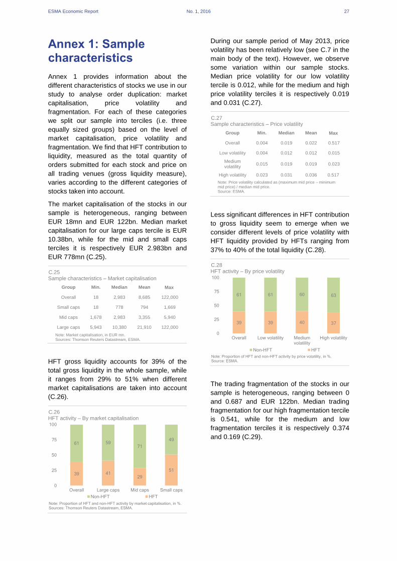
ESMA Economic Report No. 1, 2016 27
Annex 1: Sample characteristics
Annex 1 provides information about the
different characteristics of stocks we use in our
study to analyse order duplication: market
capitalisation, price volatility and
fragmentation. For each of these categories
we split our sample into terciles (i.e. three
equally sized groups) based on the level of
market capitalisation, price volatility and
fragmentation. We find that HFT contribution to
liquidity, measured as the total quantity of
orders submitted for each stock and price on
all trading venues (gross liquidity measure),
varies according to the different categories of
stocks taken into account.
The market capitalisation of the stocks in our
sample is heterogeneous, ranging between
EUR 18mn and EUR 122bn. Median market
capitalisation for our large caps tercile is EUR
10.38bn, while for the mid and small caps
terciles it is respectively EUR 2.983bn and
EUR 778mn (C.25).
C.25 Sample characteristics – Market capitalisation
Group Min. Median Mean Max
Overall 18 2,983 8,685 122,000
Small caps 18 778 794 1,669
Mid caps 1,678 2,983 3,355 5,940
Large caps 5,943 10,380 21,910 122,000
Note: Market capitalisation, in EUR mn. Sources: Thomson Reuters Datastream, ESMA.
HFT gross liquidity accounts for 39% of the
total gross liquidity in the whole sample, while
it ranges from 29% to 51% when different
market capitalisations are taken into account
(C.26).
C.26 HFT activity – By market capitalisation
During our sample period of May 2013, price
volatility has been relatively low (see C.7 in the
main body of the text). However, we observe
some variation within our sample stocks.
Median price volatility for our low volatility
tercile is 0.012, while for the medium and high
price volatility terciles it is respectively 0.019
and 0.031 (C.27).
C.27 Sample characteristics – Price volatility
Group Min. Median Mean Max
Overall 0.004 0.019 0.022 0.517
Low volatility 0.004 0.012 0.012 0.015
Medium volatility
0.015 0.019 0.019 0.023
High volatility 0.023 0.031 0.036 0.517
Note: Price volatility calculated as (maximum mid price – minimum mid price) / median mid price. Source: ESMA.
Less significant differences in HFT contribution
to gross liquidity seem to emerge when we
consider different levels of price volatility with
HFT liquidity provided by HFTs ranging from
37% to 40% of the total liquidity (C.28).
C.28 HFT activity – By price volatility
The trading fragmentation of the stocks in our
sample is heterogeneous, ranging between 0
and 0.687 and EUR 122bn. Median trading
fragmentation for our high fragmentation tercile
is 0.541, while for the medium and low
fragmentation terciles it is respectively 0.374
and 0.169 (C.29).
39 4129
51
61 5971
49
0
25
50
75
100
Overall Large caps Mid caps Small caps
Non-HFT HFT
Note: Proportion of HFT and non-HFT activity by market capitalisation, in %.Sources: Thomson Reuters Datastream, ESMA.
39 39 40 37
61 61 60 63
0
25
50
75
100
Overall Low volatility Mediumvolatility
High volatility
Non-HFT HFT
Note: Proportion of HFT and non-HFT activity by price volatility, in %.Source: ESMA.

ESMA Economic Report No. 1, 2016 28
C.29 Sample characteristics – Trading fragmentation
Group Min. Median Mean Max
Overall 0.000 0.374 0.358 0.687
Low fragmentation
0.000 0.169 0.151 0.288
Medium fragmentation
0.288 0.374 0.375 0.466
High fragmentation
0.467 0.541 0.547 0.687
Note: Trading fragmentation, calculated as Frag = 1 – HHI where HHI
is the Herfindahl-Hirschman index43.
Source: ESMA.
HFTs tend to play a more relevant role in
highly fragmented markets (42% of total gross
liquidity) compared to less fragmented markets
(27% of total gross liquidity; C.30).
C.30 HFT activity – By trading fragmentation
43 The Herfindahl-Hirschman index is computed on the
basis of the sum of squared market shares (value traded) per trading venue. A value of 1 indicates no fragmentation (all trading is on one venue), whereas lower values indicate that trading is fragmented across several trading venues. Consequently for the fragmentation index a value of 0 indicates no fragmentation (all trading is on one venue), whereas higher values indicate that trading is fragmented across several trading venues.
39 42 3727
61 58 6373
0
25
50
75
100
Overall Highfragmentation
Mediumfragmentation
Lowfragmentation
Non-HFT HFT
Note: Proportion of HFT and non-HFT activity by fragementation of trading, in %.Source: ESMA.
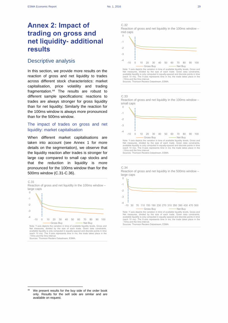
ESMA Economic Report No. 1, 2016 29
Annex 2: Impact of trading on gross and net liquidity- additional results
Descriptive analysis
In this section, we provide more results on the
reaction of gross and net liquidity to trades
across different stock characteristics: market
capitalisation, price volatility and trading
fragmentation.44 The results are robust to
different sample specifications: reactions to
trades are always stronger for gross liquidity
than for net liquidity; Similarly the reaction for
the 100ms window is always more pronounced
than for the 500ms window.
The impact of trades on gross and net
liquidity: market capitalisation
When different market capitalisations are
taken into account (see Annex 1 for more
details on the segmentation), we observe that
the liquidity reaction after trades is stronger for
large cap compared to small cap stocks and
that the reduction in liquidity is more
pronounced for the 100ms window than for the
500ms window (C.31-C.36).
C.31 Reaction of gross and net liquidity in the 100ms window – large caps
44 We present results for the buy side of the order book
only. Results for the sell side are similar and are available on request.
C.32 Reaction of gross and net liquidity in the 100ms window – mid caps
C.33 Reaction of gross and net liquidity in the 100ms window – small caps
C.34 Reaction of gross and net liquidity in the 500ms window – large caps
-4
-3
-2
-1
0
-10 0 10 20 30 40 50 60 70 80 90 100
Gross Buy Net BuyNote: Y-axis depicts the variation in time of available liquidity levels, Gross andNet measures, divided by the size of each trade. Given data constraints,available liquidity is only computed in equally-spaced and discrete points in time(each 10 ms). The X-axis represents time in ms; the trade takes place in the-10ms and the 0ms interval.Sources: Thomson Reuters Datastream, ESMA.
-4
-3
-2
-1
0
-10 30 70 110 150 190 230 270 310 350 390 430 470 500
Gross Buy Net BuyNote: Y-axis depicts the variation in time of available liquidity levels, Gross andNet measures, divided by the size of each trade. Given data constraints,available liquidity is only computed in equally-spaced and discrete points in time(each 10 ms). The X-axis represents time in ms; the trade takes place in the-10ms and the 0ms interval.Sources: Thomson Reuters Datastream, ESMA.

ESMA Economic Report No. 1, 2016 30
C.35 Reaction of gross and net liquidity in the 500ms window – mid caps
C.36 Reaction of gross and net liquidity in the 500ms window – small caps
The impact of trades on gross and net
liquidity: price volatility
The reaction of liquidity to trade events is
stronger for stocks with low price volatility
compared to stocks with high price volatility
(see Annex 1 for more details on the
segmentation of our sample with respect to
price volatility). This result confirms the
descriptive statistics showing that duplicated
orders tend to be more frequent in a low
volatility environment (C.37-C.42).
C.37 Reaction of gross and net liquidity in the 100ms window – high price volatility
C.38 Reaction of gross and net liquidity in the 100ms window – medium price volatility
C.39 Reaction of gross and net liquidity in the 100ms window – low price volatility
C.40 Reaction of gross and net liquidity in the 500ms window – high price volatility
-4
-3
-2
-1
0
-10 30 70 110 150 190 230 270 310 350 390 430 470 500
Gross Buy Net BuyNote: Y-axis depicts the variation in time of available liquidity levels, Gross andNet measures, divided by the size of each trade. Given data constraints,available liquidity is only computed in equally-spaced and discrete points in time(each 10 ms). The X-axis represents time in ms; the trade takes place in the-10ms and the 0ms interval.Sources: Thomson Reuters Datastream, ESMA.
-4
-3
-2
-1
0
-10 0 10 20 30 40 50 60 70 80 90 100
Gross Buy Net BuyNote: Y-axis depicts the variation in time of available liquidity levels, Gross andNet measures, divided by the size of each trade. Given data constraints,available liquidity is only computed in equally-spaced and discrete points in time(each 10 ms). The X-axis represents time in ms; the trade takes place in the-10ms and the 0ms interval.Source: ESMA.
-4
-3
-2
-1
0
-10 30 70 110 150 190 230 270 310 350 390 430 470 500
Gross Buy Net BuyNote: Y-axis depicts the variation in time of available liquidity levels, Gross andNet measures, divided by the size of each trade. Given data constraints,available liquidity is only computed in equally-spaced and discrete points in time(each 10 ms). The X-axis represents time in ms; the trade takes place in the-10ms and the 0ms interval.Source: ESMA.

ESMA Economic Report No. 1, 2016 31
C.41 Reaction of gross and net liquidity in the 500ms window – medium price volatility
C.42 Reaction of gross and net liquidity in the 500ms window – low price volatility
The impact of trading on gross and net
liquidity: fragmentation of trading
When fragmentation of trading is higher the
reduction of gross and net liquidity to the trade
events is stronger, in line with the descriptive
statistics showing that we observe a larger
amount of duplicated orders and a bigger
contribution of HFTs to gross liquidity in stocks
with a higher degree of trading fragmentation
(C.43-C.48; See Annex 1 for more details on
the segmentation of our sample with respect to
fragmentation of trading).
C.43 Reaction of gross and net liquidity in the 100ms window – high fragmentation
C.44 Reaction of gross and net liquidity in the 100ms window – medium fragmentation
C.45 Reaction of gross and net liquidity in the 100ms window – low fragmentation
-4
-3
-2
-1
0
-10 30 70 110 150 190 230 270 310 350 390 430 470 500
Gross Buy Net BuyNote: Y-axis depicts the variation in time of available liquidity levels, Gross andNet measures, divided by the size of each trade. Given data constraints,available liquidity is only computed in equally-spaced and discrete points in time(each 10 ms). The X-axis represents time in ms; the trade takes place in the-10ms and the 0ms interval.Source: ESMA.
-4
-3
-2
-1
0
-10 0 10 20 30 40 50 60 70 80 90 100
Gross Buy Net BuyNote: Y-axis depicts the variation in time of available liquidity levels, Gross andNet measures, divided by the size of each trade. Given data constraints,available liquidity is only computed in equally-spaced and discrete points in time(each 10 ms). The X-axis represents time in ms; the trade takes place in the-10ms and the 0ms interval.Source: ESMA.
-4
-3
-2
-1
0
-10 0 10 20 30 40 50 60 70 80 90 100
Gross Buy Net BuyNote: Y-axis depicts the variation in time of available liquidity levels, Gross andNet measures, divided by the size of each trade. Given data constraints,available liquidity is only computed in equally-spaced and discrete points in time(each 10 ms). The X-axis represents time in ms; the trade takes place in the-10ms and the 0ms interval.Source: ESMA.
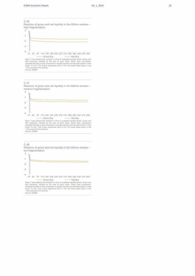
ESMA Economic Report No. 1, 2016 32
C.46 Reaction of gross and net liquidity in the 500ms window – high fragmentation
C.47 Reaction of gross and net liquidity in the 500ms window – medium fragmentation
C.48 Reaction of gross and net liquidity in the 500ms window – low fragmentation
-4
-3
-2
-1
0
-10 30 70 110 150 190 230 270 310 350 390 430 470 500
Gross Buy Net BuyNote: Y-axis depicts the variation in time of available liquidity levels, Gross andNet measures, divided by the size of each trade. Given data constraints,available liquidity is only computed in equally-spaced and discrete points in time(each 10 ms). The X-axis represents time in ms; the trade takes place in the-10ms and the 0ms interval.Source: ESMA.
-4
-3
-2
-1
0
-10 30 70 110 150 190 230 270 310 350 390 430 470 500
Gross Buy Net BuyNote: Y-axis depicts the variation in time of available liquidity levels, Gross andNet measures, divided by the size of each trade. Given data constraints,available liquidity is only computed in equally-spaced and discrete points in time(each 10 ms). The X-axis represents time in ms; the trade takes place in the-10ms and the 0ms interval.Source: ESMA.

ESMA Economic Report No. 1, 2016 33
Time series analysis
In this section we provide more details on our
regression results. As in Annex 2, we show the
results trades across different stock
characteristics: market capitalisation (C.49-
C.54), price volatility (C.55-C.60) and trading
fragmentation (C.61-C.66). In all cases the
results are displayed for the buy and sell side
of the order book.
Regression results – Market capitalisation
C.49 Regression analysis results for large caps – buy side
Coefficient Gross Liquidity
Buy
Net Liquidity
Buy
Difference
Intercept -1.24 -6.98 ***
BI0 -1.41 *** -1.14 *** -0.27 ***
BI1 -1.58 *** -1.27 *** -0.3 ***
BI2 -1.66 *** -1.34 *** -0.32 ***
BI3 -1.72 *** -1.4 *** -0.32 ***
BI4 -1.75 *** -1.43 *** -0.32 ***
BI5 -1.77 *** -1.48 *** -0.29 ***
SI0 0.47 *** 0.37 *** 0.09 ***
SI1 0.58 *** 0.44 *** 0.14 ***
SI2 0.59 *** 0.45 *** 0.15 ***
SI3 0.63 *** 0.47 *** 0.16 ***
SI4 0.64 *** 0.47 *** 0.16 ***
SI5 0.73 *** 0.54 *** 0.19 ***
Lagged spread
1101.87 *** 1968.16 ***
Volatility 893.71 *** 751.85 *** Note: The table shows the cumulative effect over time of the aggregated buy turnover changes in the gross and net liquidity across stocks and across venues for large caps. It also shows whether the difference between gross and net measures is significant or not. *** P-value<1%, ** P-value<5%, * P-value<10%. Sources: Thomson Reuters Datastream, ESMA.
C.50 Regression analysis results for large caps – sell side
Coefficient Gross Liquidity
Sell
Net Liquidity
Sell
Difference
Intercept -1.69 * -7.48 ***
SI0 -1.42 *** -1.14 *** -0.28 ***
SI1 -1.6 *** -1.29 *** -0.31 ***
SI2 -1.69 *** -1.36 *** -0.33 ***
SI3 -1.76 *** -1.42 *** -0.33 ***
SI4 -1.78 *** -1.45 *** -0.33 ***
SI5 -1.83 *** -1.52 *** -0.31 ***
BI0 0.4 *** 0.31 *** 0.09 ***
BI1 0.5 *** 0.37 *** 0.14 ***
BI2 0.53 *** 0.37 *** 0.15 ***
BI3 0.57 *** 0.4 *** 0.17 ***
BI4 0.59 *** 0.41 *** 0.17 ***
BI5 0.67 *** 0.47 *** 0.2 ***
Lagged spread
1226.72 *** 2045.87 ***
Volatility 1027.59 *** 836.22 ***
Note: The table shows the cumulative effect over time of the aggregated sell turnover changes in the gross and net liquidity across stocks and across venues for large caps. It also shows whether the difference between gross and net measures is significant or not. *** P-value<1%, ** P-value<5%, * P-value<10%. Sources: Thomson Reuters Datastream, ESMA.
C.51 Regression analysis results for mid caps – buy side
Coefficient Gross Liquidity
Buy
Net Liquidity
Buy
Difference
Intercept -24.32 -67.84
BI0 -1.33 *** -1.13 *** -0.2 ***
BI1 -1.49 -1.24 *** -0.24 ***
BI2 -1.54 -1.29 *** -0.25 ***
BI3 -1.59 *** -1.33 *** -0.26 ***
BI4 -1.6 *** -1.34 *** -0.26 ***
BI5 -1.71 *** -1.49 *** -0.23 ***
SI0 0.21 *** 0.18 *** 0.02 ***
SI1 0.23 *** 0.19 *** 0.04 ***
SI2 0.24 *** 0.2 *** 0.04 ***
SI3 0.27 *** 0.22 *** 0.04 ***
SI4 0.28 *** 0.23 *** 0.05 ***
SI5 0.4 *** 0.3 *** 0.1 ***
Lagged spread
23565.62 67174.56
Volatility 1077.56 *** 843.74 ***
Note: The table shows the cumulative effect over time of the aggregated buy turnover changes in the gross and net liquidity across stocks and across venues for mid caps. It also shows whether the difference between gross and net measures is significant or not. *** P-value<1%, ** P-value<5%, * P-value<10%. Sources: Thomson Reuters Datastream, ESMA.
C.52 Regression analysis results for mid caps – sell side
Coefficient Gross Liquidity
Sell
Net Liquidity
Sell
Difference
Intercept 125.84 47.59
SI0 -1.33 *** -1.13 *** -0.2 ***
SI1 -1.48 *** -1.25 *** -0.23 ***
SI2 -1.52 *** -1.28 *** -0.24 ***
SI3 -1.55 *** -1.31 -0.24 ***
SI4 -1.55 *** -1.31 *** -0.24 ***
SI5 -1.65 *** -1.43 *** -0.22 ***
BI0 0.19 *** 0.17 *** 0.02 ***
BI1 0.23 *** 0.19 *** 0.04 ***
BI2 0.24 *** 0.19 *** 0.05 ***
BI3 0.26 *** 0.21 *** 0.05 ***
BI4 0.28 *** 0.22 *** 0.06 ***
BI5 0.39 *** 0.29 *** 0.1 ***
Lagged spread
-126522.82 -48219.78
Volatility 2204.87 1594.19
Note: The table shows the cumulative effect over time of the aggregated sell turnover changes in the gross and net liquidity across stocks and across venues for mid caps. It also shows whether the difference between gross and net measures is significant or not. *** P-value<1%, ** P-value<5%, * P-value<10%. Sources: Thomson Reuters Datastream, ESMA.
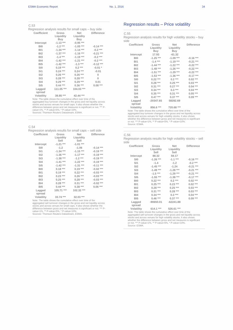
ESMA Economic Report No. 1, 2016 34
C.53 Regression analysis results for small caps – buy side
Coefficient Gross Liquidity
Buy
Net Liquidity
Buy
Difference
Intercept -1.13 *** -0.95 ***
BI0 -1.2 *** -1.05 *** -0.14 ***
BI1 -1.34 *** -1.14 *** -0.2 ***
BI2 -1.37 *** -1.16 *** -0.21 ***
BI3 -1.4 *** -1.19 *** -0.2 ***
BI4 -1.42 *** -1.21 *** -0.2 ***
BI5 -1.42 *** -1.3 *** -0.12 ***
SI0 0.19 *** 0.2 *** -0.01 *
SI1 0.24 *** 0.24 *** -0.01
SI2 0.26 *** 0.26 *** 0
SI3 0.28 *** 0.28 *** 0
SI4 0.29 *** 0.29 *** 0.01
SI5 0.44 *** 0.36 *** 0.08 ***
Lagged spread
111.05 *** 104.03 ***
Volatility 39.85 *** 42.44 ***
Note: The table shows the cumulative effect over time of the aggregated buy turnover changes in the gross and net liquidity across stocks and across venues for small caps. It also shows whether the difference between gross and net measures is significant or not. *** P-value<1%, ** P-value<5%, * P-value<10%. Sources: Thomson Reuters Datastream, ESMA.
C.54 Regression analysis results for small caps – sell side
Coefficient Gross Liquidity
Sell
Net Liquidity
Sell
Difference
Intercept -1.21 *** -1.01 ***
SI0 -1.2 -1.06 -0.14 ***
SI1 -1.34 *** -1.15 *** -0.19 ***
SI2 -1.36 *** -1.17 *** -0.19 ***
SI3 -1.38 *** -1.2 *** -0.19 ***
SI4 -1.41 *** -1.22 *** -0.19 ***
SI5 -1.42 *** -1.31 *** -0.11 ***
BI0 0.18 *** 0.19 *** -0.02 ***
BI1 0.19 *** 0.22 *** -0.03 ***
BI2 0.23 *** 0.26 *** -0.03 ***
BI3 0.25 *** 0.28 *** -0.03 ***
BI4 0.28 *** 0.31 *** -0.02 ***
BI5 0.44 *** 0.38 *** 0.06 ***
Lagged spread
105.71 *** 102.32 ***
Volatility 33.74 *** 32.03 *** Note: The table shows the cumulative effect over time of the aggregated sell turnover changes in the gross and net liquidity across stocks and across venues for small caps. It also shows whether the difference between gross and net measures is significant or not. *** P-value<1%, ** P-value<5%, * P-value<10%. Sources: Thomson Reuters Datastream, ESMA.
Regression results – Price volatility
C.55 Regression analysis results for high volatility stocks – buy side
Coefficient Gross Liquidity
Buy
Net Liquidity
Buy
Difference
Intercept 17.93 -61.32
BI0 -1.25 *** -1.09 *** -0.16 ***
BI1 -1.4 *** -1.19 *** -0.21 ***
BI2 -1.44 *** -1.22 *** -0.22 ***
BI3 -1.48 *** -1.26 *** -0.22 ***
BI4 -1.51 *** -1.29 *** -0.22 ***
BI5 -1.53 *** -1.36 *** -0.17 ***
SI0 0.22 *** 0.2 *** 0.02 ***
SI1 0.28 *** 0.25 *** 0.03 ***
SI2 0.31 *** 0.27 *** 0.04 ***
SI3 0.34 *** 0.3 *** 0.04 ***
SI4 0.35 *** 0.31 *** 0.05 ***
SI5 0.47 *** 0.37 *** 0.09 ***
Lagged spread
-20347.65 58282.69
Volatility 856.6 *** 720.68 ***
Note: The table shows the cumulative effect over time of the aggregated buy turnover changes in the gross and net liquidity across stocks and across venues for high volatility stocks. It also shows whether the difference between gross and net measures is significant or not. *** P-value<1%, ** P-value<5%, * P-value<10%. Source: ESMA.
C.56 Regression analysis results for high volatility stocks – sell side
Coefficient Gross Liquidity
Sell
Net Liquidity
Sell
Difference
Intercept 88.32 59.17
SI0 -1.26 *** -1.1 *** -0.16 ***
SI1 -1.4 -1.2 -0.2 ***
SI2 -1.45 *** -1.24 -0.21 ***
SI3 -1.49 *** -1.28 *** -0.21 ***
SI4 -1.5 *** -1.29 *** -0.21 ***
SI5 -1.55 *** -1.38 *** -0.17 ***
BI0 0.22 *** 0.2 *** 0.02 ***
BI1 0.25 *** 0.23 *** 0.02 ***
BI2 0.28 *** 0.25 *** 0.03 ***
BI3 0.31 *** 0.28 *** 0.03 ***
BI4 0.34 *** 0.3 *** 0.04 ***
BI5 0.46 *** 0.37 *** 0.09 ***
Lagged spread
-90650.01 -62241.88
Volatility 614.1 *** 526.61 *** Note: The table shows the cumulative effect over time of the aggregated sell turnover changes in the gross and net liquidity across stocks and across venues for high volatility stocks. It also shows whether the difference between gross and net measures is significant or not. *** P-value<1%, ** P-value<5%, * P-value<10%. Source: ESMA.

ESMA Economic Report No. 1, 2016 35
C.57 Regression analysis results for medium volatility stocks – buy side
Coefficient Gross Liquidity
Buy
Net Liquidity
Buy
Difference
Intercept 28.4 2.25
BI0 -1.32 *** -1.11 *** -0.21 ***
BI1 -1.49 *** -1.24 -0.26 ***
BI2 -1.54 *** -1.27 -0.27 ***
BI3 -1.59 *** -1.31 *** -0.27 ***
BI4 -1.6 *** -1.33 *** -0.27 ***
BI5 -1.65 *** -1.43 *** -0.22 ***
SI0 0.3 *** 0.26 *** 0.04 ***
SI1 0.35 *** 0.29 *** 0.06 ***
SI2 0.37 *** 0.3 *** 0.06 ***
SI3 0.39 *** 0.32 *** 0.07 ***
SI4 0.39 *** 0.32 *** 0.07 ***
SI5 0.53 *** 0.4 *** 0.14 ***
Lagged spread
-28661.69 -4178.57
Volatility 586.79 *** 477.79 ***
Note: The table shows the cumulative effect over time of the aggregated buy turnover changes in the gross and net liquidity across stocks and across venues for medium volatility stocks. It also shows whether the difference between gross and net measures is significant or not. *** P-value<1%, ** P-value<5%, * P-value<10%. Source: ESMA.
C.58 Regression analysis results for medium volatility stocks – sell side
Coefficient Gross Liquidity
Sell
Net Liquidity
Sell
Difference
Intercept 123.4 34.06
SI0 -1.33 *** -1.11 *** -0.21 ***
SI1 -1.49 *** -1.24 *** -0.25 ***
SI2 -1.54 *** -1.28 *** -0.26 ***
SI3 -1.58 *** -1.32 -0.26 ***
SI4 -1.6 *** -1.34 *** -0.26 ***
SI5 -1.64 *** -1.42 *** -0.21 ***
BI0 0.24 *** 0.21 *** 0.03 ***
BI1 0.29 *** 0.24 *** 0.05 ***
BI2 0.31 *** 0.26 *** 0.05 ***
BI3 0.34 *** 0.28 *** 0.06 ***
BI4 0.37 *** 0.3 *** 0.07 ***
BI5 0.49 *** 0.37 *** 0.12 ***
Lagged spread
-123634.27 -36042.14
Volatility 551.68 *** 439.84 *** Note: The table shows the cumulative effect over time of the aggregated sell turnover changes in the gross and net liquidity across stocks and across venues for medium volatility stocks. It also shows whether the difference between gross and net measures is significant or not. *** P-value<1%, ** P-value<5%, * P-value<10%. Source: ESMA.
C.59 Regression analysis results for low volatility stocks – buy side
Coefficient Gross Liquidity
Buy
Net Liquidity
Buy
Difference
Intercept -74.39 -16.62
BI0 -1.37 *** -1.13 *** -0.24 ***
BI1 -1.54 -1.25 *** -0.28 ***
BI2 -1.6 *** -1.31 *** -0.3 ***
BI3 -1.66 *** -1.36 *** -0.3 ***
BI4 -1.67 *** -1.37 *** -0.3 ***
BI5 -1.74 *** -1.49 *** -0.25 ***
SI0 0.35 *** 0.3 *** 0.05 ***
SI1 0.42 *** 0.33 *** 0.08 ***
SI2 0.42 *** 0.34 *** 0.08 ***
SI3 0.45 *** 0.36 *** 0.09 ***
SI4 0.46 *** 0.36 *** 0.1 ***
SI5 0.57 *** 0.43 *** 0.15 ***
Lagged spread
75257.86 14897.03
Volatility 573.33 *** 444.48 ***
Note: The table shows the cumulative effect over time of the aggregated buy turnover changes in the gross and net liquidity across stocks and across venues for low volatility stocks. It also shows whether the difference between gross and net measures is significant or not. *** P-value<1%, ** P-value<5%, * P-value<10%. Source: ESMA.
C.60 Regression analysis results for low volatility stocks – sell side
Coefficient Gross Liquidity
Sell
Net Liquidity
Sell
Difference
Intercept -93.68 -56.1
SI0 -1.37 *** -1.13 *** -0.25 ***
SI1 -1.55 *** -1.26 *** -0.29 ***
SI2 -1.6 -1.3 *** -0.3 ***
SI3 -1.64 *** -1.34 *** -0.3 ***
SI4 -1.66 *** -1.36 *** -0.3 ***
SI5 -1.73 *** -1.48 *** -0.25 ***
BI0 0.31 *** 0.26 *** 0.05 ***
BI1 0.39 *** 0.31 *** 0.08 ***
BI2 0.4 *** 0.31 *** 0.09 ***
BI3 0.43 *** 0.33 *** 0.1 ***
BI4 0.45 *** 0.34 *** 0.1 ***
BI5 0.56 *** 0.4 *** 0.15 ***
Lagged spread
94329.7 54228.21
Volatility 2121.29 1512.26 Note: The table shows the cumulative effect over time of the aggregated sell turnover changes in the gross and net liquidity across stocks and across venues for low volatility stocks. It also shows whether the difference between gross and net measures is significant or not. *** P-value<1%, ** P-value<5%, * P-value<10%. Source: ESMA.
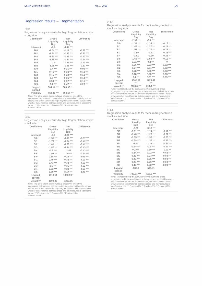
ESMA Economic Report No. 1, 2016 36
Regression results – Fragmentation
C.61 Regression analysis results for high fragmentation stocks – buy side
Coefficient Gross Liquidity
Buy
Net Liquidity
Buy
Difference
Intercept -0.6 -4.44 ***
BI0 -1.54 *** -1.17 *** -0.37 ***
BI1 -1.74 *** -1.33 *** -0.41 ***
BI2 -1.81 *** -1.38 *** -0.43 ***
BI3 -1.88 *** -1.44 *** -0.44 ***
BI4 -1.9 -1.47 *** -0.43 ***
BI5 -1.95 *** -1.58 *** -0.37 ***
SI0 0.4 *** 0.31 *** 0.09 ***
SI1 0.46 *** 0.33 *** 0.13 ***
SI2 0.45 *** 0.32 *** 0.13 ***
SI3 0.5 *** 0.36 *** 0.14 ***
SI4 0.53 *** 0.37 *** 0.15 ***
SI5 0.7 *** 0.47 *** 0.23 ***
Lagged spread
504.14 *** 866.98 ***
Volatility 359.37 *** 250.56 ***
Note: The table shows the cumulative effect over time of the aggregated buy turnover changes in the gross and net liquidity across stocks and across venues for high fragmentation stocks. It also shows whether the difference between gross and net measures is significant or not. *** P-value<1%, ** P-value<5%, * P-value<10%. Source: ESMA.
C.62 Regression analysis results for high fragmentation stocks – sell side
Coefficient Gross Liquidity
Sell
Net Liquidity
Sell
Difference
Intercept -0.6 -4.81 ***
SI0 -1.55 *** -1.18 *** -0.37 ***
SI1 -1.76 *** -1.34 *** -0.42 ***
SI2 -1.81 *** -1.38 *** -0.42 ***
SI3 -1.87 *** -1.44 *** -0.43 ***
SI4 -1.9 *** -1.47 -0.43 ***
SI5 -1.98 *** -1.6 *** -0.38 ***
BI0 0.38 *** 0.29 *** 0.09 ***
BI1 0.45 *** 0.33 *** 0.12 ***
BI2 0.43 *** 0.32 *** 0.12 ***
BI3 0.5 *** 0.36 *** 0.13 ***
BI4 0.53 *** 0.38 *** 0.15 ***
BI5 0.69 *** 0.47 *** 0.22 ***
Lagged spread
1510.11 1903.99 *
Volatility 1898.06 1293.05 Note: The table shows the cumulative effect over time of the aggregated sell turnover changes in the gross and net liquidity across stocks and across venues for high fragmentation stocks. It also shows whether the difference between gross and net measures is significant or not. *** P-value<1%, ** P-value<5%, * P-value<10%. Source: ESMA.
C.63 Regression analysis results for medium fragmentation stocks – buy side
Coefficient Gross Liquidity
Buy
Net Liquidity
Buy
Difference
Intercept -2.33 *** -3.7 ***
BI0 -1.31 *** -1.14 *** -0.16 ***
BI1 -1.47 *** -1.27 *** -0.21 ***
BI2 -1.54 *** -1.32 *** -0.22 ***
BI3 -1.59 -1.37 -0.22 ***
BI4 -1.61 -1.39 -0.22 ***
BI5 -1.69 *** -1.53 *** -0.16 ***
SI0 0.21 *** 0.2 *** 0
SI1 0.25 *** 0.23 *** 0.02 ***
SI2 0.27 *** 0.24 *** 0.02 ***
SI3 0.28 *** 0.26 *** 0.03 ***
SI4 0.28 *** 0.26 *** 0.03 ***
SI5 0.4 *** 0.31 *** 0.09 ***
Lagged spread
1365.51 ***
1729.41 ***
Volatility 710.85 *** 611.1 ***
Note: The table shows the cumulative effect over time of the aggregated buy turnover changes in the gross and net liquidity across stocks and across venues for medium fragmentation stocks. It also shows whether the difference between gross and net measures is significant or not. *** P-value<1%, ** P-value<5%, * P-value<10%. Source: ESMA.
C.64 Regression analysis results for medium fragmentation stocks – sell side
Coefficient Gross Liquidity
Sell
Net Liquidity
Sell
Difference
Intercept -0.86 -3.16 ***
SI0 -1.31 *** -1.14 *** -0.17 ***
SI1 -1.48 *** -1.26 *** -0.22 ***
SI2 -1.55 *** -1.32 *** -0.23 ***
SI3 -1.59 *** -1.36 *** -0.23 ***
SI4 -1.61 -1.38 *** -0.23 ***
SI5 -1.68 *** -1.5 *** -0.17 ***
BI0 0.2 *** 0.19 *** 0.01 **
BI1 0.24 *** 0.22 *** 0.02 ***
BI2 0.26 *** 0.23 *** 0.03 ***
BI3 0.29 *** 0.25 *** 0.04 ***
BI4 0.29 *** 0.26 *** 0.04 ***
BI5 0.42 *** 0.32 *** 0.09 ***
Lagged spread
-938.1 508.41
Volatility 749.34 *** 658.9 *** Note: The table shows the cumulative effect over time of the aggregated sell turnover changes in the gross and net liquidity across stocks and across venues for medium fragmentation stocks. It also shows whether the difference between gross and net measures is significant or not. *** P-value<1%, ** P-value<5%, * P-value<10%. Source: ESMA.

ESMA Economic Report No. 1, 2016 37
C.65 Regression analysis results for low fragmentation stocks – buy side
Coefficient Gross Liquidity
Buy
Net Liquidity
Buy
Difference
Intercept -24.94 -71.15
BI0 -1.08 -1 *** -0.08 ***
BI1 -1.18 *** -1.06 *** -0.12 ***
BI2 -1.21 *** -1.08 *** -0.12 ***
BI3 -1.23 *** -1.11 *** -0.12 ***
BI4 -1.24 *** -1.11 *** -0.12 ***
BI5 -1.24 *** -1.14 *** -0.1 ***
SI0 0.25 *** 0.24 *** 0.01 **
SI1 0.34 *** 0.31 *** 0.02 ***
SI2 0.38 *** 0.35 *** 0.03 ***
SI3 0.39 *** 0.36 *** 0.03 ***
SI4 0.4 *** 0.36 *** 0.03 ***
SI5 0.47 *** 0.41 *** 0.06 ***
Lagged spread
24099.17 70200.06
Volatility 973.28 *** 804.43 ***
Note: The table shows the cumulative effect over time of the aggregated buy turnover changes in the gross and net liquidity across stocks and across venues for low fragmentation stocks. It also shows whether the difference between gross and net measures is significant or not. *** P-value<1%, ** P-value<5%, * P-value<10%. Source: ESMA.
C.66 Regression analysis results for low fragmentation stocks – sell side
Coefficient Gross Liquidity
Sell
Net Liquidity
Sell
Difference
Intercept 131.11 49.71
SI0 -1.08 *** -1.01 *** -0.07 ***
SI1 -1.17 *** -1.08 *** -0.1 ***
SI2 -1.2 *** -1.1 *** -0.1 ***
SI3 -1.21 *** -1.11 *** -0.1 ***
SI4 -1.22 *** -1.12 *** -0.1 ***
SI5 -1.23 *** -1.15 *** -0.07 ***
BI0 0.18 *** 0.18 *** 0
BI1 0.23 *** 0.22 *** 0.01 **
BI2 0.29 *** 0.28 *** 0.01 ***
BI3 0.29 *** 0.27 *** 0.01 ***
BI4 0.32 *** 0.3 *** 0.02 ***
BI5 0.38 *** 0.34 *** 0.04 ***
Lagged spread
-132536.52
-51140.78
Volatility 566.25 *** 477.64 ***
Note: The table shows the cumulative effect over time of the aggregated sell turnover changes in the gross and net liquidity across stocks and across venues for low fragmentation stocks. It also shows whether the difference between gross and net measures is significant or not. *** P-value<1%, ** P-value<5%, * P-value<10%. Source: ESMA.