economic review - fraser

Vol. 31, No. 1

ECONOMIC REVIEW

1995 Quarter 1

Restoring Generational v / 2Balance in U.S. Fiscal Policy:What Will It Take?by Alan J. Auerbach,Jagadeesh Gokhale,and Laurence J. Kotlikoff

Vagueness, Credibility, and 1 3Government Policyby Joseph G. Haubrich

Federal Funds Futures as an Indicator of Future Monetary Policy: A Primerby John B. Carlson,Jean M. Mclntire, and James B. Thomson

20

FEDERAL RESERVE BANK OF CLEVELAND

Digitized for FRASER http://fraser.stlouisfed.org/ Federal Reserve Bank of St. Louis

■

E C O N O M I C R E V I E W

1995 Quarter 1 Vol. 31, No. 1

Restoring Generational 2 Balance in U.S. Fiscal Policy: What Will It Take?by Alan J. Auerbach, Jagadeesh Gokhale, and Laurence J. Kotlikoff

What are the magnitudes of tax increases, transfer cuts, or reductions in government purchases required to restore a generationally balanced U.S. fiscal policy? Under the authors' conservative baseline of updated generational accounts, income taxes would have to be raised permanently by 43 percent, federal transfers cut by 33 percent, or government purchases lowered by 32 percent beginning in 1996. The required policy changes will be larger if their implementation is postponed. The authors also find that the outlay reductions in nondefense and non-Social Security spending that Congress recently considered would still leave an unsustainably large imbalance in the generational stance of U.S. fiscal policy.

Vagueness, Credibility, and Government Policyby Joseph G. Haubrich

1 3

This article examines the economic reasons why it may be in a government agency’s — and society's— best interest to be vague about policy objectives. The author uses the recently developed concept of "cheap talk" to explain that when an agency faces a trade-off between precise and credible announcements, its best move may be to provide truthful but limited information.

Federal Funds Futures as an 2 0Indicator of Future Monetary Policy: A Primerby John B. Carlson, Jean M. Mclntire, and James B. Thomson

Unlike most futures contracts, which are drawn on commodities or financial instruments whose price or yield is determined in competitive markets, the federal funds futures rate is essentially determined by a deliberative decision of the Federal Open Market Committee (FOMC). As such, the fed funds futures market is a place where one can place a bet as to what future monetary policy will be. The FOMC can thus assess in fairly precise terms what markets expect it to do. In this paper, the authors examine the predictive accuracy of the fed funds futures market and consider some policy implications. They find that accuracy clearly improves in the two-month period leading up to the contract's expiration and that the largest prediction errors occur around policy turning points.

Economic Review is published quarterly by the Research Department of the Federal Reserve Bank of Cleveland. Copies of the Review are available through our Corporate Communications & Community Affairs Department. Call 1-800-543- 3489 (OH, PA, WV) or 216-579- 2001, then immediately key in 1-5-3 on your touch-tone phone to reach the publication request option. If you prefer to fax your order, the number is 216-579-2477.

Coordinating Economist: Jagadeesh Gokhale

Advisory Board:Charles T. Carlstrom Joseph G. Haubrich Peter Rupert

Editors: Tess Ferg Robin Ratliff

Design: Michael Galka Typography: Liz Hanna

Opinions stated in Economic Review are those of the authors and not necessarily those of the Federal Reserve Bank of Cleveland or of the Board of Governors of the Federal Reserve System.

Material may be reprinted provided that the source is credited. Please send copies of reprinted material to the editors.

ISSN 0013-0281


2

Restoring Generational Balance in U.S. Fiscal Policy: What Will It Take?

by Alan J. Auerbach, Jagadeesh Gokhale, and Laurence J. Kotlikoff Alan J. Auerbach is a profes

sor of economics at the University of California, Berkeley, and an associate of the National Bureau of Economic Research; Jagadeesh Gokhale is an economic advisor at the Federal Reserve Bank of Cleveland; and Laurence J. Kotlikoff is a professor of economics at Boston University and an associate of the National

Bureau of Economic Research. The authors thank the Office of Management and Budget for providing critical data on FY1996 budget projections and the Social Security Administration for providing population projections. They also thank Robert Anderson, Darrel Cohen, Robert Kilpatrick, and Patrick Locke for helpful comments.

Introduction

Generational accounting is a relatively new method o f reorganizing the government’s budget data to understand how the burden of paying for government spending on goods and services is distributed among living and future generations.1 To study this distribution, generational accounting estimates lifetime net tax rates facing different generations under current policies.2 For a given generation, the lifetime net tax rate is its per capita lifetime net tax burden as a share o f the present value o f its per capita lifetime labor income.

The lifetime net tax burden, in turn, is the present value o f per capita taxes net o f transfers that members o f a generation pay over their lifetimes, evaluated as of their year of birth. For generations currently alive, the lifetime net tax burden includes net taxes they

■ 1 The technique of generational accounting was developed in Auerbach, Gokhale, and Kotlikoff (1991) and in Kotlikoff (1992). See also Auerbach, Gokhale, and Kotlikoff (1994). Unless stated otherwise, spending in this paper refers to government purchases of goods and services.

■ 2 A generation is defined as individuals of a particular sex born in the same year.

have paid in the past and those they may ex pect to pay in the future. Similar remarks apply to the calculation o f the present value of a g en eration’s per capita lifetime labor income.

In contrast to the three previous years, a generational accounting analysis of U.S. fiscal policy was not included in the Budget of the United States for fiscal year 1996.3 This paper presents such an analysis. It reports updated lifetime net tax rates using the latest long-range tax and expenditure projections made by the Office o f Management and Budget (OMB).4

Earlier presentations of lifetime net tax rates indicated that current U.S. fiscal policy contains a large generational imbalance — a result that this update confirms. If the current fiscal treatment o f living (including newborn) generations continues throughout their lifetimes, the lifetime net tax rate on those born in 1993 would be about 34 percent, while future generations

■ 3 The last generational accounting presentation in the U.S. Budget appeared in Office of Management and Budget (1994), chapter 3.

■ 4 These projections are an extension of the OMB's 1994 Mid-Session Review baseline projection and incorporate, among other things, longterm demographic and fiscal projections of the Social Security Administration and the Health Care Financing Administration


3

would face an average rate of 84 percent."’That is, under current policies, future generations would bear a fiscal burden two-and-a-half times as large, on average, than that on the current newborn generation. Further, a sizable fiscal imbalance remains despite incorporating optimistic assumptions about the path of future federal purchases and health care outlays in the calculations. Such large projected fiscal burdens on future generations imply that current fiscal policy is "unsustainable"— a conclusion that is robust to alternative assumptions about future productivity growth and interest rates.

This method of calculating the imbalance in U.S. fiscal policy has been criticized on several grounds. One objection focuses on the assumption that living generations will continue to be treated per current fiscal policy throughout their lifetimes, while the tax treatment of those bom in the future w ill differ. To some, this assumption seems to imply that the incidence of future policy changes to correct the imbalance would fall exclusively on future generations. They suggest that the calculations be altered to include the impact of future policy changes on the lifetime net tax rates of living generations, since this will normally be the case. Then, they contend, lifetime net tax rates on future generations would decline from the high levels suggested in earlier generational accounting presentations to more plausible and acceptable levels, and most of the dramatic conclusions drawn by generational accounting would disappear.6

The assumption o f unchanged tax treatment o f living generations was only a heuristic and was not intended to suggest that future policy changes will apply only to future generations. Nevertheless, this paper responds to the criticism directly by posing a question: What are the magnitudes o f tax increases, transfer cuts, or spending reductions necessary to equalize the lifetime net tax rates o f current newborn and future generations — that is, to restore a generationally balanced fiscal policy?

The experiments assume that policy changes, when introduced, will apply to all generations alive then and in every year thereafter. Hence, the new policies will affect the lifetime net tax rates of most generations alive in 1993, our base year. The tax, transfer, and spending policy experiments are conducted for a set of baseline projections o f future revenues and outlays as well as for alternative assumptions about the growth paths of federal purchases and health care outlays. In each case, we report the changes in taxes, transfers, or purchases needed to equalize lifetime net tax rates of future and current

newborn generations. We also present the values of the equalized lifetime net tax rates.

The calculated tax hikes, transfer reductions, or spending cuts required for achieving a generationally balanced fiscal policy are immense — much larger than those recently considered by Congress as part o f the debate to balance the budget by the year 2002. Thus, achieving a balanced budget by that date would not place U.S. fiscal policy on a sustainable path unless budget balance were preserved thereafter. The reason is that under current projections, growth in outlays after 2002 will far outstrip growth in revenues, and maintaining a balanced budget beyond 2002 is likely to require cuts in addition to those needed just to balance the budget by that year.

The policy changes required to equalize lifetime net tax rates of newborn and future generations can be viewed as alternative measures of the imbalance in current U.S. fiscal policy. Unlike the critics’ conjecture, these measures also suggest that a substantial imbalance is em bedded in current U.S. fiscal policy.

I. How Are Generational Accounts and Lifetime Net Tax Rates Computed?7

Generational accounts refer to the present value of taxes net o f transfers that a member of each generation may expect to pay on average now and in the future. Thus, generational accounts reveal the prospective net tax burdens on different generations. In contrast, lifetime generational accounts include net taxes paid in the past and refer to the present value of net taxes as of the generation’s year o f birth.

■ 5 The estimates presented in Office of Management and Budget (1994), chapter 3, were 36.3 percent on current (1992) newborns and 82 percent on future generations. The differences in the estimates reported here stem from technical improvements incorporated in the calculations as well as from the use of previously unavailable long-range budgetary projections provided by the 0MB. The lifetime net tax rates reported are averaged across male and female generations.

■ 6 For examples of such criticism, see Eisner (1994) and Haveman (1994). Another criticism, not dealt with here, stems from the Ricardian equivalence proposition, which states that current generations, perceiving the tax increases on future generations implicit in the deficit financing of current government spending, will respond by increasing their saving and bequests. However, formal tests fail to detect the altruistic behavior required for Ricardian equivalence. See Altonji, Hayashi, and Kotlikoff (1992).

■ 7 This section presents a brief discussion of the method of generational accounting. For more detailed treatments, see Auerbach, Gokhale, and Kotlikoff (1991) and Kotlikoff (1992). See also Office of Management and Budget (1994), chapter 3.


A. Living Generations

Lifetime generational accounts are used here to compute the lifetime net tax rate facing each generation bom between 1900 and 1993- The calculations use National Income and Product Account data on federal, state, and local taxes, transfers, and spending for each year up to 1993, as well as OMB projections of these aggregates up to 2030.8

In the computational procedure, total taxes and expenditures are classified into several categories for each year between 1900 and 2030. We include taxes on incomes from labor and capital, payroll taxes, and indirect taxes. Expenditures refer to transfers such as Social Security, Medicare, Medicaid, and other welfare payments, plus government purchases. The amount in each tax and transfer category is distributed among generations alive in a certain year— cohorts by single year of age and sex ranging from newborn to 100 years old. For years prior to and including 1993, we use actual population data to perform this distribution; for future years, we use population projections from the Social Security Administration.9

The amounts of per capita taxes or transfers distributed to members o f each generation are determined according to relative profiles of tax payments and transfer receipts obtained from microeconomic surveys.10 Current and past taxes and transfers are distributed among different generations using available information on age- and sex-specific payments and receipts for those years. For some categories, such as Social Security transfers, relative profiles are available for each year between I960 and 1992. For others, profiles are available for only a few of the years. For each payment and receipt category, the earliest available profile is used for distributing payments and receipts in prior years. Similarly, the latest available profile is used to distribute the amounts in later (including future) years.

For years beyond 2030, we project the per capita amounts of taxes and transfers by applying a growth factor to the values for the year

■ 8 All outlays and receipts are measured in 1993 dollars.

■ 9 We use the intermediate population projections through 2066 made by the Social Security Administration. We then extend these projections through 2200 using the mortality, fertility, and immigration assumptions applicable in 2066.

■ 10 These surveys include the Survey of Consumer Expenditures by the Bureau of Labor Statistics, the Survey of Income and Program Participation by the Bureau of the Census, the Current Population Survey by the Bureau of the Census, the Annual Abstracts of the Social Security Bulletin by the Social Security Administration, and the Survey of Consumer Expenditures by the Federal Reserve System.

2030. The prospective generational account for each current (1993) generation is computed by subtracting total transfer receipts from total tax payments in each future year that the generation will be alive, actuarially discounting the resulting net tax payments back to 1993 using an assumed rate of interest, r, and summing over the remaining years of life for that generation.

The computation of the lifetime generational account for a given generation alive in 1993 uses the same type of calculation, except that net taxes paid in the past are also included. Moreover, the annual net taxes are actuarially discounted back to the generation’s year of birth. In the case of the generation aged 43 in 1993 (those bom in 1950), for example, per capita net taxes paid up to 1993 and projected net taxes paid up to 2050 (age 100) are capitalized to yield a generational account as of 1950.

The present value of lifetime labor income is used as a base to calculate the lifetime net tax rate for each generation. As mentioned earlier, the lifetime net tax rate is the lifetime gen erational account as a percent of the present value of lifetime labor income. For each generation, the stream of per capita labor income earned in each year up to 1993 and projected income for future years is capitalized to produce the present value of lifetime labor income. We derive the estimates of per capita labor income in a manner similar to that for deriving per capita taxes and transfers: In each year, labor’s share of net national income is distributed by relative profiles of labor incom e These profiles are based on individual wage and salary data from the Census Bureau’s Current Population Survey and are constructed for the years 1963 through 1992.

The implications of current fiscal policy for th e lifetime net tax rates on future generations (those born after 1993) can be derived by using the accounts of generations currently alive. T h is computation requires a consideration of the government’s intertemporal budget constraint which can be specified as

(1) PVSPEND, = GWt + PVCt + PVFt.

Equation ( 1) states that the present value of the government’s current and projected purchases, PVSPEND' , must equal the government’s current net worth, GWt, plus the present value of prospective net tax payments o f all generationsDigitized for FRASER

http://fraser.stlouisfed.org/ Federal Reserve Bank of St. Louis

5

currently alive, PVC,, plus the present value of net tax payments of all future generations,PVFt . The sum of prospective generational accounts over all individuals currently alive provides an estimate o f PVFt .

We estimate the value of PVSPENDt by computing the present value of current and projected government spending on goods and services. Projections of purchases through 2030 assume that government purchases will keep pace with population growth and with increases in labor productivity. Spending projections beyond 2030 are made by applying a growth factor to per capita spending in 2030. Under the assumption that the 2030 spending per capita will be maintained thereafter (except for an adjustment for growth), aggregating the per capita amounts across the (projected) population for years beyond 2030 yields total spending for these years.

The per capita amounts of purchases in 2030 are obtained by dividing the 2030 value o f total purchases into one general and three age-specific categories and distributing these equally across the relevant (projected) population segments for the year 2030. Finally, we estimate GWt by cumulating annual government deficits over time.11 For the United States, the value o f GWt is negative because government budgets have been in deficit for most years during the last several decades.

Knowing three o f the four terms in equation( 1 ) enables us to derive the remaining item, PVFt , as a residual. Thus, PVFt is the amount o f the present value of government purchases not covered by current government net worth plus the present value of current and future net tax payments by living generations. This residual must be paid for by net tax payments to be levied on generations as yet unborn.

Although the manner in which the residual burden will be distributed across unborn generations is unknown today, we can illustrate its magnitude by distributing it according to some predetermined rule. Here, we adopt the criterion that the distribution should equalize the lifetime net tax rates of all future generations. This requires that the residual burden be distributed equally across all future generations except for an adjustment for growth.12 Thus, generations born in year t pay net tax burdens 1 + g times the net tax burdens of generations born in year t - 1 , where g is the annual rate o f growth of labor productivity.13 Because future labor income is assumed to grow at rate g, this adjustment imposes equal lifetime net tax rates on all future generations.

A comparison of the lifetime net tax rate on future generations with that on newborn generations is one way to estimate the degree of generational imbalance embedded in current fiscal policy. The lifetime net tax rate on new born generations is derived by finding the ratio of the present value o f their net tax payments under current policy projections to the present value of their lifetime labor incomes. If a growth- adjusted distribution of the residual burden among future generations produces a lifetime net tax rate significantly larger than that on current newborns, fiscal policy can be viewed as being biased against future generations. If the lifetime net tax rate on future generations is judged as being prohibitively high, current fiscal policy may be deemed unsustainable.

II. Generational Accounts and Lifetime Net Tax Rates for the United States

A. ProspectiveGenerationalAccounts

Baseline prospective generational accounts for selected generations alive in 1993 are shown in tables 1 and 2. The calculations include all federal, state, and local government taxes, transfers, and spending on goods and services and assume that government spending on goods and services will keep pace with population and productivity growth. They also incorporate conservative estimates of growth in government

■ 11 This method does not include the value of government physical assets in GWt . However, if it did, one would have to include the present value of imputed rent on these assets in PVSPEND,, representing the government's purchase of the service flow from these assets for public consumption. Because these two items would be equal in present value, constraint (1) would be unaffected.

■ 12 Equal Bbsolute distribution of the residual burden would successively reduce the lifetime net tax rates on generations born later because continued productivity growth will cause their labor income to exceed that of generations born earlier. A growth-adjusted distribution of the residual burden would result in the imposition of equal lifetime net tax rates on all future generations. For a further discussion of these issues, see Kotlikoff and Gokhale (1994).

■ 13 We assume that the ratio of per capita net tax burdens on future male and female generations is the same as that on newborns.


6

T A B L E 1

The Composition of Male Generational Accounts ( r * 0.06, g ■ 0.012)(present values in thousands of 1993 dollars)

Taxes Paid Transfers Received

Generation'sAge in 1993

Net Tax Payment

LaborIncomeTaxes

CapitalIncomeTaxes

PayrollTaxes

ExciseTaxes

SocialSecurity Health Welfai

0 87.2 39.9 9.6 38.3 34.4 8.8 22.4 3.95 107.0 49.1 12.1 47.6 40.0 10.8 26.2 4.9

10 130.3 60.0 15.1 59.0 46.0 12.8 30.8 6.315 159.6 73-4 19.1 73.4 52.5 14.7 36.1 8.020 188.7 86.6 24.1 88.1 57.0 16.6 40.6 9.725 199.9 92.2 28.5 94.5 57.2 19.8 42.4 10.330 195.7 90.8 33.7 93.0 56.0 23.6 44.2 9.935 182.7 86.1 39.9 88.0 54.6 28.8 47.8 9.340 158.6 77.9 44.9 79.7 53.3 35.5 53.2 8.6»5 119.7 65.7 47.6 67.6 50.1 43.5 59.8 7.950 68.0 50.5 48.0 52.4 45.7 53.9 67.4 7.355 7.1 33.9 46.0 35.4 40.2 67.0 74.7 6.660 -57 .0 18.0 42.3 18.9 34.0 83.6 80.8 5.965 -105.1 7.2 37.2 7.2 28.2 93.5 86.3 5.170 -108 .3 3.1 29.4 3.2 22.6 85.5 76.6 4.575 - 100.8 1.6 19.7 1.6 17.1 71.5 65.6 3.7HO -86 .3 0.9 9.9 1.0 12.0 54.5 52.8 2.785 -76 .2 0.6 0.0 0.7 8.0 42.3 41.4 1.890 -5 8 .9 0.5 0.0 0.5 6.4 33.5 31.4 1.4Future 215.5 — — — — — — —

generations’1Percentage Difference in Net Payments

Future 147.1 — — — — — — —generationsand age zero____________________

a. Generations bom in 1994 and thereafter. SOURCE: Authors calculations.

health care outlays. The growth of Medicare and Medicaid expenditures averaged 7.4 and 15.5 percent, respectively, over the last five years. The baseline incorporates a rapid growth in these outlays until 2005, with somewhat slower growth thereafter.14

The prospective net tax burdens shown in tables 1 and 2 exhibit a pronounced life-cycle pattern. Working-age generations, who are in their high earning and taxpaying years, have positive net tax burdens: The present values of their income, payroll, and indirect taxes are large, but values of receipts from Scxial Security and health care transfers are small. The opposite result holds true for older generations.

In 1993, newborn males may expect to pay $87,200, and newborn females $53,2(X), on net, under baseline policies during their remaining

lifetimes. In contrast, average lifetime net tax burdens amount to $215,500 for future males and $131,500 for future females if the fiscal treatment of living generations continues under baseline policies.

As mentioned earlier, prospective generational accounts can be combined with past net tax payments to calculate lifetime net tax burdens for all living generations. Taken as fractions of lifetime labor incomes, they yield lifetime net tax rates Table 3 shows baseline lifetime gross and net tax rates and gross transfer rates for generations

■ 14 Post-2005 growth rates for Medicare and Medicaid outlays arethe OMB's best estimates. The growth rates used in all calculations are available from the authors upon request.


D

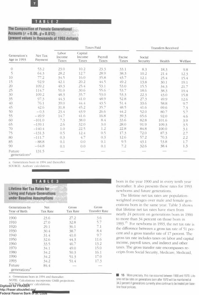
T A B L E 2

The Composition of Female Generational Accounts ( r = 0.06, 0 = 0 .0 1 2 ) (present values in thousands of 1993 dollars)

Taxes Paid Transfers Received

Generation’s Age in 1993

Net Tax Payment

LaborIncomeTaxes

CapitalIncomeTaxes

PayrollTaxes

ExciseTaxes

SocialSecurity Health Welfare

0 53.2 23.0 10.2 23.3 33.1 8.3 18.3 9.85 64.3 28.2 12.7 28.9 38.3 10.2 21.4 12.3

10 77.2 34.5 16.0 35.8 43.7 12.1 25.4 15.415 92.9 42.1 20.2 44.5 49.2 13.8 30.1 19.120 109.2 49.3 25.4 53.1 53.0 15.5 34.3 21.725 114.7 51.0 30.6 55.6 53.7 18.6 38.3 19.430 109.2 48.3 35.7 53.0 53.3 22.3 43.0 15.835 97.3 4 4 .3 41.0 48.9 52.8 27.3 49.9 12.640 76.1 39.0 44.4 43.5 51.4 33.6 58.8 9.745 42.6 31-8 45.2 35.7 48.5 41.6 69.6 7.350 - 0 .3 23.4 43.9 26.6 44.2 52.0 80.7 5.755 -4 9 .9 14.7 41.6 16.8 39.3 65.6 92.0 4.660 - 101.0 7.3 38.0 8.4 33.6 82.8 101.6 3.965 -139.1 2.6 32.0 3.0 28.0 91.9 109.3 3.570 -140 .4 1.0 22.5 1.2 22.8 84.8 100.0 3.175 -131 .3 0.5 12.4 0.5 17.3 72.0 87.3 2.780 -111 .7 0.3 4.7 0.3 12.6 57.2 70.3 2.285 - 88.8 0.1 0.0 0.1 9.5 43.1 53.8 1.790 -6 4 .8 0.1 0.0 0.1 7.2 32.6 38.4 1.3Future 131.5 — — — — — — —

generations11

a. Generations lx>m in 1994 and thereafter. SOURCE: Authors' calculations.

T A B L E 3

Lifetime Net Tax Rates Living and Future Generationsunder Baseline Assumptions

Generations by Net Ciross GrossYear of Birth Tax Rate Tax Rate Transfer Rate

1900 23.6 27.2 3.61910 27.0 32.8 5.71920 29.1 36.1 7.11930 30.4 38.7 8.41940 31.4 41.0 9.71950 32.6 44.3 11.61960 33.5 46.7 13.21970 34.1 49.0 15.01980 34.2 50.3 16.11990 34.2 51.3 17.01993 34.2 51.4 17.3Future 84.4 — —

generations3

a. Generations tx>m in 1994 and thereafter.NOTE: Calculations incorporate OMB projections.SOURCE: Authors’ calculations.

bom in the year 1900 and in every tenth year thereafter. It also presents these rates for 1993 newborns and future generations.

The lifetime net tax rates are population- weighted averages over male and female generations born in the same year. Table 3 shows that lifetime net tax rates have risen from nearly 24 percent on generations born in 1900 to more than 34 percent on those bom in 1993.15 For newborns in 1993, the net tax rate is the difference between a gross tax rate of 51 percent and a gross transfer rate of 17 percent. The gross tax rate includes taxes on lalx>r and capital income, payroll taxes, and indirect and other taxes. The gross transfer rate encompasses receipts from Social Security, Medicare, Medicaid,

■ 15 More precisely, this rise occurred between 1900 and 1970. Lifetime net tax rates on generations born after 1970 will be maintained at 34.2 percent if generations currently alive continue to be treated per baseline fiscal policies.Digitized for FRASER


8

1 T A B L E 4

Lifetime Net Tax Rates for Living and Future Generations under Alternative Health Care and Federal Spending Paths

Slower Health Care

and Spending Growth

Generations by Year of Birth Baseline

SlowerSpendingGrowth3

SlowerHealth

CareGrowthb

1900 23.6 23.6 23.6 23.61910 27.0 27.0 27.1 27.01920 29.1 29.1 29.2 29.21930 30.4 30.4 30.7 30.71940 31.4 31.4 31.9 31.91950 32.6 32.6 33.4 33.41960 33.5 33-5 34.4 34.41970 34.1 34.1 35.3 35.31980 34.2 34.2 35.7 35.71990 34.2 34.2 36.0 36.01993 34.2 34.2 36.0 36.0

Future 84.4 73.1 70.4 59.1generations0

a. Federal spending is held constant in real terms after the year 2000.b. Health care spending grows at a 2 percent slower rate than the baseline through 2005, followed by baseline growth.c. Generations bom in 1994 and thereafter.NOTE: Calculations incorporate OMB projections.SOURCE: Authors' calculations.

T A B L E 5

Percentage Difference under Alternative Interest and Growth Rates: Baseline

0.0178 = 0.007 0.012

r =0.03 120 119 1220.06 158 147 1370.09 280 261 243

SOURCE: Authors’ calculations.

T A B L E 6

Percentage Difference under Alternative Interest and Growth Rates: Slower Health Care Growth and Constant Real Federal Purchases

8 = 0.007 0.012 0.017

r =0.03 49 43 380.06 72 64 570.09 149 137 125

SOURCE: Authors’ calculations.

and other welfare transfers. The lifetime net tax rate on future generations is a staggering 84 percent, which is almost two-and-a-half times as large as that on newborns in 1993.16

Table 4 reports lifetime net tax rates under alternative future paths for outlays on health care and federal purchases. Specifically, column 1 o f table 4 repeats the baseline lifetime net tax rates of table 3. Column 2 shows the e ffect of freezing real federal spending on goods and services permanently beginning in 2000. Lifetime net tax rates of all living generations are unchanged, since neither future tax nor transfer payments are affected by this policy. However, because reducing federal purchases lessens the residual burden on future generations, their lifetime net tax rate is lowered to 73 percent. This result suggests that freezing federal purchases permanently is not sufficient to put the U.S. fiscal house in order from a gen erational accounting perspective.

Column 3 of table 4 reports the effect of assuming a 2 percent slower growth in health care outlays until 2005, with baseline growth thereafter. Slower growth in health care spending raises the lifetime net tax rates of young and middle- aged living generations — those who will receive lower health care transfers as a result. It also reduces the lifetime net tax rate on future generations by 14 percentage points. Thus, although slower growth in government health care expenditures over the next decade will reduce the generational imbalance in U.S. fiscal policy, a sizable imbalance may still remain.

Column 4 of table 4 shows the effect of com bining the policies of columns 2 and 3 — an optimistic scenario. This reduces the lifetime net tax rate on future generations from 84 percent to 59 percent. Thus, even if federal purchases are not increased beyond current levels and growth in health care outlays is 2 percentage points lower than the baseline over the next 10 years, future generations will incur lifetime net tax rates that are 64 percent larger, on average, than those facing current newborns.

The baseline and other policies discussed so far use a 6 percent rate of discount (r = 0.06) and a 1.2 percent rate of average productivity growth (g = 0.012) to project taxes, transfers, and

■ 16 Note that future generations'lifetime net tax rate is derived bydistributing the residual of the present value of government spending after government net worth and the net contribution of living generations have been deducted. Hence, it cannot be subdivided into gross tax and transfer rates.


9

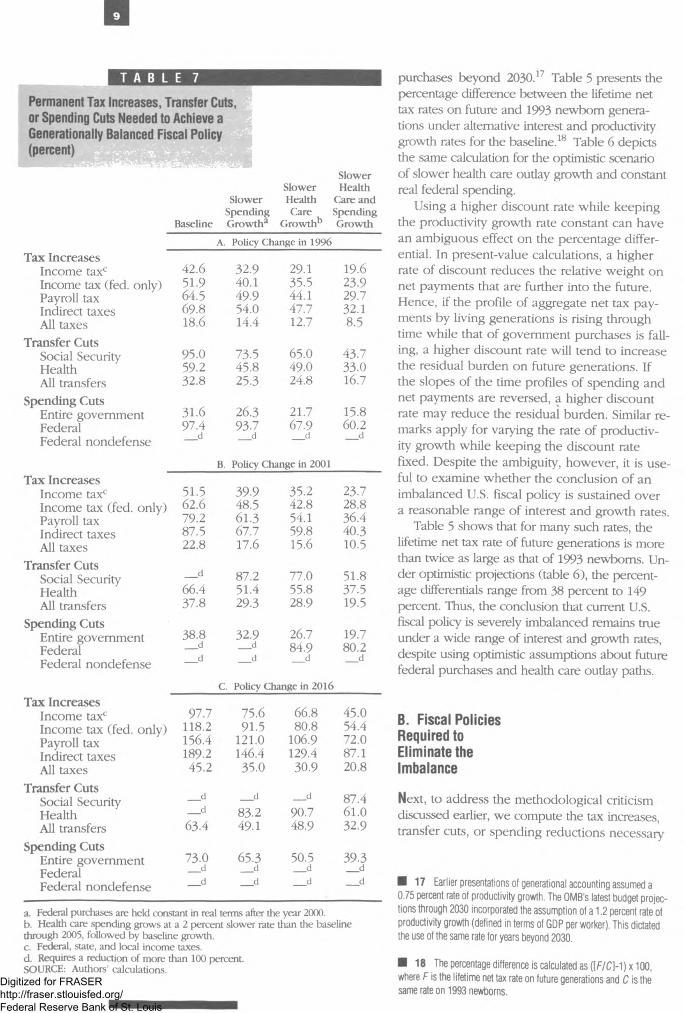
T A B L E 7

Permanent Tax Increases, Transfer Cuts, or Spending Cuts Needed to Achieve a Generationally Balanced Fiscal Policy (percent)

Slower

Tax IncreasesIncome taxc Income tax (fed. only) Payroll tax Indirect taxes All taxes

Transfer CutsSocial SecurityHealthAll transfers

Spending CutsEntire government FederalFederal nondefense







Slower HealthSlower Health Care and

Spending Care SpendingBaseline Growth3 Growth*5 Growth

A. Policy Change in 1996

42.6 32.9 29.1 19.651.9 40.1 35.5 23.964.5 49.9 44.1 29.769.8 54.0 47.7 32.118.6 14.4 12.7 8.5

95.0 73.5 65.0 43.759.2 45.8 49.0 33.032.8 25.3 24.8 16.7

31.6 26.3 21.7 15.897.4 93.7 67.9 60.2__ d __ d __ d __ d

B. Policy Change in 2001

51.5 39.9 35.2 23.7i 62.6 48.5 42.8 28.8

79.2 61.3 54.1 36.487.5 67.7 59.8 40.322.8 17.6 15.6 10.5

__ d 87.2 77.0 51.866.4 51.4 55.8 37.537.8 29.3 28.9 19.5

38.8 32.9 26.7 19.7__ d __ d 84.9 80.2__ d __ d __ d __ d

C. Policy Change in 2016

97.7 75.6 66.8 45.0i 118.2 91.5 80.8 54.4

156.4 121.0 106.9 72.0189.2 146.4 129.4 87.1

45.2 35.0 30.9 20.8

__ d __ d __ d 87.4__ d 83.2 90.7 61.063.4 49.1 48.9 32.9

73.0d

65.3d

50.5d

39.3 __d

a. Federal purchases are held constant in real terms alter the year 2000.b. Health care spending grows at a 2 percent slower rate than the baseline through 2005, followed by baseline growth.c. Federal, state, and local income taxes.d. Requires a reduction of more than 100 percent.SOURCE: Authors’ calculations.

purchases beyond 2030.17 Table 5 presents the percentage difference between the lifetime net tax rates on future and 1993 newborn generations under alternative interest and productivity growth rates for the baseline.18 Table 6 depicts the same calculation for the optimistic scenario of slower health care outlay growth and constant real federal spending.

Using a higher discount rate while keeping the productivity growth rate constant can have an ambiguous effect on the percentage differential. In present-value calculations, a higher rate o f discount reduces the relative weight on net payments that are further into the future. Hence, if the profile of aggregate net tax payments by living generations is rising through time while that of government purchases is falling, a higher discount rate will tend to increase the residual burden on future generations. If the slopes of the time profiles of spending and net payments are reversed, a higher discount rate may reduce the residual burden. Similar remarks apply for varying the rate o f productivity growth while keeping the discount rate fixed. Despite the ambiguity, however, it is useful to examine whether the conclusion o f an imbalanced U.S. fiscal policy is sustained over a reasonable range of interest and growth rates.

Table 5 shows that for many such rates, the lifetime net tax rate of future generations is more than twice as large as that of 1993 newborns. Under optimistic projections (table 6), the percentage differentials range from 38 percent to 149 percent. Thus, the conclusion that current U.S. fiscal policy is severely imbalanced remains true under a wide range of interest and growth rates, despite using optimistic assumptions about future federal purchases and health care outlay paths.

B. Fiscal Policies Required to Eliminate the Imbalance

Next, to address the methodological criticism discussed earlier, we compute the tax increases, transfer cuts, or spending reductions necessary

■ 17 Earlier presentations of generational accounting assumed a0.75 percent rate of productivity growth. The OMB’s latest budget projections through 2030 incorporated the assumption of a 1.2 percent rate of productivity growth (defined in terms of GDP per worker). This dictated the use of the same rate for years beyond 2030.

■ 18 The percentage difference is calculated as ((f/C l-1 ) x 100, where F is the lifetime net tax rate on future generations and C is the same rate on 1993 newborns.


10

T A B L E 8

Equalized Lifetime Net Tax Rates for Newborn and Future Generations Resulting from Table 7 Policies (percent)







Tax IncreasesIncome taxc Income tax (fed. onl Payroll tax Indirect taxes All taxes



Baseline

SlowerSpendingGrowth*

SlowerHealthCare

Growthb

Slower Health

Care and Spending Growth

A. Policy Change in 1996

42.7 40.8 41.9 39.9, 42.8 40.9 41.9 40.0

43.9 41.7 42.6 40.544.8 42.4 43.3 40.943.6 41.5 42.4 40.3

38.1 37.2 38.7 37.839.9 38.6 39.8 38.639.7 38.5 39.8 38.5

34.2 34.2 36.0 36.034.2 34.2 36.0 36.0__d __d __d __d

B. Policy Change in 2001

44.5 42.2 43.1 40.844.6 42.2 43.1 40.846.0 43.4 44.1 41.546.4 43.6 44.4 41.645.4 42.9 43.7 41.2

__d 37.6 39.1 38.140.4 39.0 40.2 38.840.4 39.0 40.3 38.9

34.2 34.2 36.0 36.0__d __d 36.0 36.0__d __d __d __d

C. Policy Change in 2016

52.5 48.4 48.6 44.5) 52.6 48.4 48.6 44.5

55.6 50.8 50.7 45.951.7 47.8 48.0 44.153.2 48.9 49.0 44.8

__d __d __d 38.8__d 40.8 41.8 39.943.0 41.0 42.0 40.0

34.2 34.2 36.0 36.0__d __d __d __d__d __d __d __d

a. Federal purchases are held constant in real terms after the year 2000.b. Health care spending grows at a 2 percent slower rate than the baseline through 2005, followed by baseline growth.c. Federal, state, and local income taxes.d. Requires a reduction of more than 100 percent.SOURCE: Authors’ calculations.

to eliminate the generational imbalance in U.S. fiscal policy. Various combinations of all three policies are introduced beginning in 1996,2001, and 2016. Because the new policies are applicable to all generations alive when they are introduced, they will affect the lifetime net tax rates of most living generations. In each case, we calculate the permanent percentage increase (or reduction) required in taxes, transfers, or purchases in order to equalize the lifetime net tax rates o f 1993 newborn and future generations.

Panel A of table 7 presents the percentage by which various taxes, transfers, and spending will have to change beginning in 1996 to eliminate the generational imbalance. The required percentage increases are shown for the baseline and for the alternative federal spending and health care outlay growth paths analyzed in table 4. Under baseline projections, incom e tax revenues would have to increase permanently by almost 43 percent beginning in 1996 to equalize the lifetime net tax rates of newborn and future generations. This implies that the average income tax rate would have to rise from 15.7 percent currently to 22.3 percent immediately and permanently.

Under the fortuitous case of slow growth in health care outlays and zero growth in federal purchases, income taxes would have to increase by about 20 percent. If only federal income taxes are considered, the required increases in annual revenues range between 24 and 52 percent; those necessary under payroll or indirect tax hike policies are even larger. If all taxes are considered, eliminating the imbalance in U.S. fiscal policy would require tax hikes of about 19 percent under baseline projections and 8.5 percent under the optimistic scenario.

Cuts in transfers to establish equal lifetime net tax rates on newborn and future generations would also be severe. Under the baseline projection, a 33 percent permanent and across-the- board reduction in transfers beginning in 19% would be necessary to restore a generationally balanced policy. Alternatively, restoring balance would require permanently reducing the size o f combined federal, state, and local government purchases by 32 percent beginning in 1996.

Table 8 shows the value at which the lifetime net tax rates on 1993 newborns and future generations would be equalized under the corresponding policies shown in table 7. Under baseline projections, for example, increasing all taxes permanently by 19 percent beginning in 1996 would raise the lifetime net taxes of 1993 newborns from 34 percent to 44 percent and


T A B L E 9

Impact of the Balanced Budget Proposal by the Year 2002 on Lifetime Net Tax Rates of Living and Future Generations

Generations by Year of Birth Baseline

BalancedBudget

Proposal Difference151900 23.6 23.6 0.01910 27.0 27.1 0.11920 29.1 29.2 0.11930 30.4 30.6 0.21940 31.4 31.7 0.31950 32.6 33.1 0.51960 33.5 34.0 0.51970 34.1 34.8 0.71980 34.2 35.2 1.01990 34.2 35.2 1.01993 34.2 35.1 0.9Future generations1 84.4 72.5 -1 1 .9

a. Present value of lifetime net taxes as a ratio of the present value of lifetime labor income.b. Percentage-point increase in the net tax rate if the balanced budget proposal is adopted.c. Generations born in 1994 and thereafter.SOURCE: Authors’ calculations.

reduce that on future generations from 84 percent to 44 percent. That is, increasing all taxes permanently by 19 percent is equivalent to increasing lifetime net tax rates of 1993 newborns by almost 30 percent. Note that the equalized lifetime net tax rates on newborn and future generations are different for different policies. If an across-the-board transfer cut were adopted instead of an across-the- board tax hike, lifetime net tax rates on newborn and future generations would be equalized at 40 percent instead of 44 percent.

Delaying policy changes to restore a generationally balanced fiscal policy is likely to prove costly. This can be seen from panels B and C in tables 7 and 8. Raising income taxes beginning in 2001 instead of in 1996 will necessitate an increase o f 52 percent instead of 43 percent. Similarly, initiating cuts in government purchases in 2001 instead of in 1996 will deepen the cuts to 39 percent from 32 percent. Introducing these policies in 2016 will push the required income-tax hike to 98 percent and will increase the cuts required in government purchases to 73 percent.

The same is true for all other tax increases and transfer or spending cuts. Indeed, some spending and transfer cuts that will restore generational balance if implemented in 1996 are no longer feasible if implemented in 2001 or 2016 because the required cuts would exceed

100 percent. For example, eliminating health care transfers entirely beginning in 2016 would not be sufficient to restore a generationally balanced policy.

The required hikes in taxes or cuts in transfers and spending to restore generational eq uity are quite considerable. The main message of this section is that no matter how one chooses to calculate it, the mammoth size of the imbalance in U.S. fiscal policy cannot be made to disappear. Moreover, policy changes to correct the imbalance need to be introduced sooner rather than later: Procrastination will only make the medicine more bitter.

III. The Balanced Budget Amendment

This section contrasts the policies required for restoring generational balance in fiscal policy with those being considered by policymakers today. While debating the adoption of a balanced budget amendment to the U.S. Constitution, Congress recently considered proposals to cut all outlays except for defense and Social Security. Here, we consider the impact of similar cuts on the generational stance o f U.S. fiscal policy. The outlay reductions involve cuts in nondefense discretionary spending ranging from 1 percent in 1996 to 4 percent in 2002 from our baseline values. For Medicare and Medicaid, the reductions range from 3 percent in 1996 to 14 percent in 2002. Finally, cuts in other mandatory spending categories range from 4 percent in 1996 to 16 percent in 2002. For each category, the percentage cut for 2002 is preserved in later years.19

Table 9 shows the impact of this proposal on the lifetime net tax rates of living and future generations. The rates are higher for living, especially younger, generations. The rate for generations born in 1950, for example, increases by 0.5 percent, while that for 1993 newborns is almost 1 percentage point higher.The proposal would imply a reduction in the lifetime net tax rate of future generations from 84 to 73 percent.

The outlay cuts analyzed here redress the imbalance to some extent, but still leave an unsustainably large lifetime net tax rate on future generations. Thus, under what we consider to

■ 19 These cuts balance the federal budget by the year 2002 from a “current law” baseline in which federal discretionary spending is frozen in nominal terms. Under our conservative baseline, however, the budget remains in deficit in all future years.Digitized for FRASER


be conservative but reasonable budget projections, future Congresses may need to rein in outlays or increase revenues further to restore generational balance to U.S. fiscal policy.Given the results of the previous section, leaving such large adjustments for future consideration is likely to prove costly.

IV. Conclusion

The generational stance of current U.S. fiscal policy is badly out o f balance. It is impossible to avoid this conclusion no matter which of many alternative measures one uses to analyze the generational distribution of net tax burdens. Although tax cuts seem to have widespread political appeal today, the analysis presented here suggests that enacting them may be the wrong thing to do.

In fact, the early adoption o f fiscal measures to reduce the projected heavy net tax burdens on future generations is imperative. This requires either increasing taxes or reducing government outlays today. Redressing the current U.S. fiscal imbalance is important because such heavy burdens will prove economically infeasible to impose on future generations in view of the fact that gross tax rates would have to be higher than net tax rates. Moreover, imposing high lifetime net tax burdens on future generations may depress their incentives to work, save, and invest, thereby hurting future Americans’ living standards. Finally, the analysis shows that postponing the adoption of corrective measures will only worsen the choices available to policymakers in the future.

References

Altonji, Joseph, Fumio Hayashi, and Laurence J. Kotlikoff. “Is the Extended Family Altruistically Linked? Direct Tests Using Micro Data,” American Economic Review, vol. 82, no. 5 (Decem ber 1992), pp. 1177 - 98.

Auerbach, Alan J., Jagadeesh Gokhale, and Laurence J . Kotlikoff. “Generational Accounts: A Meaningful Alternative to Deficit Accounting,” in David Bradford, ed., Tax Policy an d the Economy, vol. 5. Cambridge, Mass.: MIT Press and the National Bureau o f Economic Research, 1991, pp. 5 5 -1 1 0 .

------------ »--------------» and_________ . “Generational Accounts and Lifetime Tax R ates__1900-1991,” Federal Reserve Bank o f Cleveland, Economic Review, vol. 29, no. 1 (Quarter 1 1993), pp. 2 - 1 3 .

------------ >------------- » and__________ “Generational Accounting: A Meaningful Way to Evaluate Fiscal Policy,” Journal o f Economic Perspectives, vol. 8, no. 1 (Winter 1994), pp. 7 3 -9 4 .

Eisner, Robert. “The Grandkids Can Relax,”The Wall Street Journal, November 9, 1994.

Haveman, Robert. “Should Generational Accounts Replace Public Budgets and Deficits?” Journal o f Economic Perspectives, vol. 8, no. 1 (Winter 1994), pp. 9 5 -1 1 1 .

Kotlikoff, Laurence J. Generational Accounting: Knowing Who Pays, an d When, f o r What We Spend. New York: The Free Press, 1992.

------------ , and Jagadeesh Gokhale. “Passing theGenerational Buck,” The Public Interest, no. 114 (Winter 1994), pp. 7 3 -8 1 .

Office of Management and Budget. Analytical Perspectives, Budget o f the United States Government, Fiscal Year 1995. Washington,D C.: U.S. Government Printing Office, 1994


13

Vagueness, Credibility, and Government Policy

by Joseph G. Haubrich Joseph G. Haubrich is an economist and consultant at the Federal Reserve Bank of Cleveland. The author thanks Loretta Mester for helpful comments.

Introduction

Have more than thou showest,Speak less than thou knowest,Lend less than thou owest.

— William Shakespeare, King Lear

(Act I, sc. iv, line 132)

Should the Federal Reserve — or any other government agency — make precise statements about its policy objectives? Determining the proper amount of secrecy in government generates controversy whether the agency involved undertakes espionage, banking, or monetary policy. Between the broad areas of agreement (classifying military strategies, publishing legislation) lie equally broad areas of contention.

This article explores the econom ic reasons why a government agency may find it in its own — and society’s — interest to be vague about policy objectives. Circumstances arise in which it is optimal for agencies to release only partial information about their decisions. For that reason, vagueness, and the secrecy necessary to preserve it, represent an accommodation with an imperfect world rather than a conspiracy o f silence.

Unlike complaints about the Central Intelligence Agency or the National Security Agency, the objections against banking and monetary authorities center not around a total lack of public announcements, but around the vagueness of their policy statements. This results from three related but separable policies: closed meetings, delayed release of decisions and minutes, and uninformative releases. Immediate release of a videotaped meeting may matter little if the policies agreed upon remain vague and imprecise, while a blacked-out, highly secret meeting could in principle result in detailed, precise statements of policy.

In the area o f banking regulation, Irvine Sprague, a former director of the Federal Deposit Insurance Corporation (FDIC), described his ambiguity about announcing which banks were too big to fail: “Comptroller Todd Conover hinted that the eleven largest banks in the nation were immune from failure. In my Boston speech, I identified the top two as being absolutely safe. The right number is elusive.” 1

■ 1 See Sprague (1986), p. 259.Digitized for FRASER http://fraser.stlouisfed.org/ Federal Reserve Bank of St. Louis

14

Closure policy is not the only area where banking rules seem vague, nor do regulators have a monopoly on ambiguity. Regulatory enforcement of commercial lending standards — a serious concern during the last recession— has also been criticized for imprecision (McLemore [1991]). In the realm of monetary policy, Congressman Henry B. Gonzalez, former chairman of the House Banking Committee, has called for videotaping Federal Open Market Committee (FOMC) meetings and for the immediate release of monetary policy objectives. Outside the government, credit-rating agencies do not always announce precise standards for each rating (Hansell [19931). More recently, both types of ambiguity have surfaced in the area of derivatives. There is apparently still some uncertainty about how regulators will treat bank investment in derivatives (Karr and. Gaylord [1994]) and about what banks will tell their customers (Tomasula [1994]).

In this article, I explore the concept technically known as “cheap talk” as a simple economic reason for secrecy and vagueness. Cheap talk illustrates an incompatibility between precision and credibility in policy announcements and provides an econom ic explanation of why such announcements provide a limited, but still real, amount of information. The cheap- talk explanation for secrecy emphasizes the cooperative nature of the problem. In that respect, it differs greatly from the vagueness and secrecy of a lazy worker hiding from his boss or of a junta trying to keep its human rights violations from the press. Cheap talk presents an agency that wants to communicate, but that for reasons detailed below', cannot do so with perfect precision.

This article presents a simple example of points first raised by Stein (1989), along with an intuitive introduction to the econom ic theory of cheap talk. It then uses some recent advances to look at why Stein’s arguments for secrecy may fail and why precise announcements would be useful.2

■ 2 Other authors have suggested different reasons for vagueness and secrecy. See Goodfriend (1986) and Kane (1980) for a more detailed examination of this issue.

■ 3 Signaling works, then, when its benefits outweigh its costs— but things don't always happen that way. Economists thus distinguish between “separating" equilibria, where different types split out, and “pooling" equilibria, where everyone acts the same. See Spence (1973).

I. Cheap Talk and Communication

"Then you should say what you m ean , ” the March Hare went on. “I do, "Alice hastily replied; “at least— at least I mean u 'hat I sa\— ”

— Lew is Carroll, Alice 's Adventures in Wonderland

Secrecy and vagueness describe aspects of communication. Consequently, any econom ic theory of secrecy and vagueness must address the economics o f communication. The facet that appears most useful, and that I therefore concentrate on, is technically called cheap talk. Cheap talk refers to unverifiable messages that are costless to send and receive. This stands in contrast to “signaling,” a better-known economic theory o f communication that refers to messages which are both costly and verifiable.

Signaling builds on the intuition o f "put your money where your mouth is.” The eco nomics of signaling, for instance, explain why a company will erect a costly headquarters to demonstrate its intent to stay around, or why skilled workers undertake the expense o f a co llege education to distinguish themselves from less skilled workers. In each case — construction or education — the costly action serves notice of something important, such as dependability or quality. Every firm wishes to appear reliable, and every worker w ishes to appear highly skilled. Those w'ith a true advantage differentiate themselves by bearing the cost o f signaling, which acts as a device to screen out less desirable types.3

Cheap talk, in contrast, arises when different types do not wish to appear the same and when there is no costly investment option. An example here would be the classified ads. Nothing prevents me from listing a piano for sale, but it serves no purpose if I really wish to sell my comic hxx)k collection. Likewise, a SBF (single black female) would most likely not list herself as a DJM (divorced Jewish male), though in principle she could.

More abstractly, the communication envisioned by cheap-talk theory involves a sender and a receiver. The sender has private information that matters to the receiver, w ho must choose an action. The outcome depends on both the sender’s type (that is, the private information the sender has) and the action taken by the receiver. Thus, a receiver’s action might be to visit my house writh the intent to buy my comic book collection.


15

T A B L E 1

Coordination Game

R eceiver

Sender

T yp e a T yp e b

Action A

2,30,0

Action B

0,02,3

A ction C

1,2

1.2

SOURCE: Adapted from Matthews, OkunoFujiwara, and Postlewaite (1991).

F I G U R E 1

Utility Functions

m+b

This sort o f communication or coordination game has been justified here with rather homey examples o f pianos, comic books, and malls, but it has a direct bearing on policy announcements. Consider a central bank that, for whatever reason (internal politics, the latest economic research), has a particular position on how much banks should rely on discount-window borrowing for short-term liquidity. An easy central bank would let banks borrow substantial amounts at short notice. Banks, if they knew this, would want to structure their loan portfolios to exploit this possibility. A tough central bank would discourage lending, and if banks were aware of that, they would not want to be caught short. In this case, it benefits the central bank to communicate its position to the banks — that is, to declare whether it is type a (easy) or type b (tough) in the game of figure 1 .

To take another example, a regulator may look at low-capitalized financial institutions, such as savings and loans, and decide how it wants to deal with their risky investments.One type of regulator may prefer to prosecute management vigorously for undertaking what it deems to be inappropriate risks, while another type may view denying those investments as an unfair hardship on a well-mn organization. Clearly, it matters to the thrift owners — and to their investment strategy — which position the regulator takes. Just as clearly, the regulator is much more likely to get its way by talking cheaply and revealing its type to the industry.

The classified ad example pinpoints one big advantage of cheap talk: coordination. It wastes everyone’s time if aspiring pianists, rather than X-men aficionados, com e to my house. Likewise, agreeing on a place to meet if one gets separated from a group of friends at the mall gives another simple example of the advantages of cheap talk as coordination.

Table 1 describes the coordination role of cheap talk in the formalism of game theory. The sender may Ix.1 type a or type b, while the receiver may take action A, B, or C. The first number of each pair denotes the payoff to the sender; the second is the payoff to the receiver. If the sender does not send a message about his type, the receiver takes action C, because the certain payoff of 2 beats the average of 1.5 from choosing A or B in ignorance. The sender, however, has an incentive to send a message — and to send the taith — because delivering the wrong message hurts the sender as well as the receiver. If a type a sender announces “I’m type b." then both the sender and receiver get zero.1

II. Secrecy and Vagueness: The Partition Equilibrium

Men use ... speech only to conceal their thoughts.

— Voltaire, Dialogue 14. Le Chapon et la Poularde

In the previous section, cheap talk served a coordinating role, being both credible and precise. Vagueness and secrecy had no place. This section describes a more subtle effect in which

■ 4 Even in this simple example, things are not as straightforward as they seem. For example, another cheap-talk equilibrium exists in which the receiver ignores all messages, and hence the sender can report any arbitrary message. Game theorists accurately describe this as the babbling equilibrium, which points out another difficulty with cheap-talk games: They often have several equilibria, only one of which may have the desired properties. The example also leaves unspecified the language of the messages, whether verbal, code, or the number of lamps left in the tower of Boston’s Old North Church. Readers interested in a deeper treatment of these issues should consult Matthews, Okuno-Fujiwara, and Postlewaite (1991).Digitized for FRASER


16

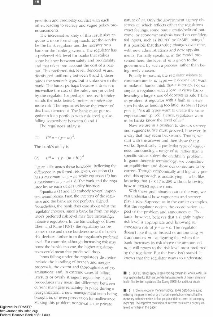
precision and credibility conflict with each other, leading to secrecy and vague policy pronouncements.

The increased subtlety of this result also requires a more formal approach. Let the sender be the bank regulator and the receiver be a bank or the banking system. The regulator has a preferred risk level for banks that strikes some balance between safety and profitability and that takes into account the cost of a bailout. This preferred risk level, denoted m and distributed uniformly between 0 and 1 , determines the sender’s type, but is unknown to the bank. The bank, perhaps because it does not internalize the cost o f the safety net provided by the regulator (or perhaps because it understands the risks better), prefers to undertake more risk. The regulators know the extent of this bias, denoted b. The bank must put together a loan portfolio with risk level y, also falling somewhere between 0 and 1 .

The regulator’s utility is

(1) UR= - ( y ~ m )2.

The bank’s utility is

(2) UB = - { y - [m + b ] ) 2

Figure 1 illustrates these functions. Reflecting the difference in preferred risk levels, equation ( 1)has a maximum at y = m, while equation (2) has a maximum at y = tn+ b. The bank and the regulator know each other’s utility function.

Equations (1) and (2) embody several important assumptions. First, the interests of the regulator and the bank are not perfectly aligned. Nonetheless, the bank does care about what the regulator chooses, since a bank far from the regulator’s preferred risk level may face increasingly intrusive regulation. In the terminology of Buser, Chen, and Kane (1981), the regulatory tax becomes more and more burdensome as the bank’s risk deviates further from the regulator’s preferred level. For example, although increasing risk may boost the bank’s income, the higher regulatory taxes could mean that profits will drop.

Items falling under the regulator’s discretion include the handling of branch and merger proposals, the extent and thoroughness o f examinations, and, in extreme cases o f failure, lawsuits or overly stringent regulation. Such procedures may mean the difference between current managers remaining in place during a reorganization, a new management team being brought in, or even prosecution for malfeasance. Making this problem nontrivial is the private

nature o f m. Only the government agency observes m, which reflects either the regulator’s exact feelings, some bureaucratic/political outcome, or econom ic analysis based on confidential inputs, such as BOPEC or CAMEL ratings.^It is possible that this value changes over time, with new administrations and new appointments. Formally speaking, in the model presented here, the level o f m is given to the government by such a process, rather than being freely chosen.

Equally important, the regulator wishes to communicate its m type — it doesn’t just want to make all banks think that it is tough. For example, a regulator with a low m views banks investing a large share o f deposits in safe T-bills as prudent. A regulator with a high m views such banks as lending too little. As Stein (1989) puts it, “Not all types want to create the same expectations” (p. 36). Hence, regulators want to let banks know the level of m 6

Now we are in a position to discuss secrecy and vagueness. We must proceed, however, in a way that may seem backwards. That is, we start with the answer and then show that it works. Specifically, a particular type of vagueness, announcing a range o f m rather than a specific value, solves the credibility problem.In game-theoretic terminology, we conjecture an equilibrium and show our conjecture to be correct. Though economically and logically precise, this approach is unsatisfying — a bit like knowing that 17 X 17 is 289 without knowing how to extract square roots.

With these preliminaries out of the way, we can understand how vagueness and secrecy play a role. Suppose, as in the earlier examples, that the regulator notices the coordination aspect of the problem and announces m. The bank, however, believes that a slightly higher risk level is appropriate and, knowing m, chooses a risk o f y = m + b. The regulator doesn’t like this, so instead of announcing m, it announces m - b, figuring that when the bank increases its risk above the announced m, it will return to the risk level most preferred by the regulator. But the bank isn't stupid. It knows that the regulator wants to understate

■ 5 BOPEC ratings apply to bank holding companies, while CAMEL ratings apply to banks. Both are confidential assessments of these institutions’ health filed by their regulators. See Spong (1990) for additional details

■ 6 In Stein's model of monetary policy, some distortion (caused either by the government or by a market imperfection) means that the monetary authority wishes to fool people and drive down the unemployment rate. The imperfect correlation of interests thus takes a slightly different form than in this paper.Digitized for FRASER


Dm, so it overstates y even more. Understanding this, the regulator wants to understate m further yet, meaning that the bank adjusts risk y up even more, meaning that the regulator .... Obviously, credibly communicating m proves impossible. Because the regulator has an incentive to manipulate banks' expectations, it cannot credibly and precisely announce its preferred risk level. Divergent interests make this impossible.7

Banks and regulators have similar, but not identical, interests. This makes communication desirable, but precise announcements useless. On the other hand, it makes imprecise — or vague — announcements useful. Suppose that instead of announcing that the preferred risk for banks is m = 0.57721, the regulator simply announces whether its preferred risk is high, medium, or low. Because interests are not identical, the regulator wants to manipulate banks’ expectations. However, because interests are similar, a regulator with a high preferred risk (large m) will not manipulate expectations too far. It will not want to tell banks that its preferred risk is in the low category, since the difference is just too large.With only three choices, the coordination side of communication becomes more important than the manipulation side. The regulator in effect commits itself to not telling little white lies — only big lies are possible. And while the regulator wishes that its hard-charging loan machine would take a little less risk, it really doesn't want the bank to become a conservative bond investor.

More formally, consider the regulator announcing a “partition” of three intervals [0, « ,], [av a 21, and [a2, 1]. (For completeness, I define the first and last terms as a 0=0 and « 3= 1 .) W henever m falls between 0 and a v the regulator announces that it favors low risk, or that m is in the interval [0, a t).

For any such announcement, the bank, knowing m has a uniform distribution, makes a best

dj + cii + jguess o f it a s ------2------an<J consequently

chooses its risk level as

(3) y -a i + a >+1 , u 8 -------- ---------+ o.

The bank pushes up its risk level by b from its best guess of the regulator’s true m. For example, whenever m falls between 0 and a x, the bank sets

each region. It must be true that if m falls in the interval [ap a i+ 1], the regulator prefers to announce that particular interval rather than any other.

At the boundaries, an arbitrage condition holds: The regulator, with a target risk level of tn - a i , must be indifferent between announcing interval [ai _ v a i ] or [at , a i+1 ]. From equations ( 1) and (3), this condition becom es

a . + a.^,(4) - (^ - J m + b _ a y

_ a i - i + a i 2 ------2------+ b - a.) .

Equation (4) reduces to a difference equation having the form a i+1 = 2a i - a i_ 1 - 4 b , subject to a 0 = 0 and a } = 1.

Standard methods exist to solve such difference equations (see Goldberg [1958]), and using them delivers the results

a l = — + 4b and

2 / , a2 = - + 4b.

If we set b = then the three intervals (or partitions) become low = [ 0, \ ], medium = [ ± J-], and high = [ 1 ], Notice the asymmetry in this partition equilibrium. The intervals are not all the same size, meaning that the regulator can be more precise when its preferred risk level exceeds the mean (that is, when m > -|). Because the bank tends to set risk above what the regulator prefers, the regulator can use the natural endpoint, m = 1 , to create a more precise announcement. The result is that announcements will be vaguer and secrecy will be higher when the regulator’s risk is relatively low.

These numbers make the example particularly simple, but the main points carry through in general. The number and size of the partitions may vary as the exact trade-off between coordination and manipulation changes. Thus, partitions remain, as does the asymmetry between them.

To summarize, the regulator wishes to com municate its preferred risk level to the bank. The gaming caused by the bank desiring more

y = T + b

In order to show that this vagueness tactic actually works, we need to be more specific and calculate the a- s, or the boundaries for

■ 7 This scenario assumes that the interaction is a one-shot game. Considering repeated interactions between the bank and the regulator may lead to different results, but only, as Stein (1989) notes, under very strong assumptions.

■ 8 This analysis closely follows Crawford and Sobel (1982). Banks choose y to maximize their expected utility, given by equation (2).


18

risk than does the regulator means that any precise announcement will not be credible. The partition equilibrium, on the other hand, delivers a credible announcement that is not precise.

III. Small Lies and Small Banks

Striving to better, oft we m ar what 's well.— William Shakespeare,

King Lear (Act I, sc. iv, line 371)

The partition equilibrium provides an intuitive justification for secrecy and vagueness. It represents a way to communicate credibly when interests are similar but not identical. A closer look at the reasoning involved, however, casts some doubt on the general applicability of the results. Because an exacting analysis of the criticisms would involve some highly technical aspects inappropriate for an Economic Review, this section concentrates on economic intuition instead.

The first problem concerns how the regulator (sender) tries to influence the receiver. In the partition example, if the regulator announces that it prefers medium risk, the bank guesses that m = ~ (because ^ 1 ] = | ) an< ̂chooses a

risk level of y = § + ^ = § • This response may tempt the regulator into announcing a "revised” message of " m is in the interval (y-j’ ^)- If the bank reasons as before, this will lead to a risk

level of y =The bank may not reason as before, how

ever. The original partition equilibrium defined the ranges, but w hat if the sender changes the announced range? What does the bank believe when the regulator does something unexpected? This puts the economist in the uncomfortable position of playing psychologist. It also makes the ultimate result somewhat uncertain. For example, if the bank recognizes what the regulator is doing with the revised announcement, it will shade its choice of y somewhat higher, the regulator will shade the interval lower, and the partition equilibrium will break down. As the originator of this critique explains, "The cheap-talk equilibrium breaks down entirely if small differences in government announcements can cause only small differences in public expectations” (Conlon [19941, p. 420).

An unexpected announcement can have various consequences.9 When the regulator

announces that m is in the interval | ) , theM2 6bank may believe, "Things are totally fouled up. W e’d better assume that m = Such a be

lief will once again allow the partition equilibrium to exist. That is, the regulator realizes that any deviation from the standard announcement could lead to an undesirably large change in bank expectations. In this case, because the bank becom es too conservative, it would be better for the regulator to stay with its original three announcements.

Another critical assumption is that the regulator faces only one bank, or a completely homogeneous banking system that acts like one bank.If, instead, many banks each have different preferred risk levels (bjs), problems can once again arise. In this case, if the regulator makes an unexpected announcement, the average of the potentially different responses may lead to a sm(X)th response. Any big shifts get averaged out. and the equilibrium again unravels.10

Put another way, with a large audience, the sender has an incentive to "fine tune” the average audience reaction. This leads receivers to attempt to offset the anticipated fine tuning, and communication breaks down.

IV. Conclusion

He was a power politically fe r years, but be never got prominent enough t ’ have bis speeches garbled.

— Abe Martin.A be Martin s Sayings an d Sketches

How much detail a government should com municate to its citizens remains controversial, especially in the areas of money and banking. On many issues, the gov ernment communicates to foster coordination with the public. There are simply some things it is useful for citizens to know, and the government tells them. In other cases where interests may not align exactly, communication cannot always be both precise and credible. Vagueness and secrecy present one way around the problem by allowing partial communication.

The conflict between credibility and precision suggests that pressuring an agency to release information may not always be productive. Releasing bank regulators’ meeting notes or

■ 9 This is the problem of multiple equilibria, mentioned in footnote 4

■ 10 See Conlon (1992) The detailed argument is quite complexDigitized for FRASER http://fraser.stlouisfed.org/ Federal Reserve Bank of St. Louis

19

videotaping FOMC deliberations will most likely result in reports and videotapes displaying the lamented vagueness o f current official releases. The partition equilibrium remains the optimal solution to the problem facing the government and the public; videotaping will not change the trade-off between vagueness and credibility.

Pressure may result in truthful, precise announcements if it leads to an appropriate change in institutional structure. The change must somehow further align the interests o f the two parties or introduce a credible commitment mechanism. Less drastic changes, perhaps occurring as agencies com e to grips with the trade-offs involved, may alter the amount of information released. The FOMC's recent policy announcements are a case in point.11

These conclusions should be treated with a healthy skepticism, however. As we have seen, further examination of the econom ic issues reveals that the benefits o f vagueness may be sensitive to particular modeling assumptions. Cheap talk represents an intriguing, but not entirely compelling, justification for imprecise policy announcements.

References

Buser, Stephen A., Andrew H. Chen, and Edward J. Kane. “Federal Deposit Insurance. Regulatory Policy, and Optimal Bank Capital," Jou rnal o f Finance, vol. 35. no. 1 (March 1981), pp. 51 - 60.

Conlon, John R. “Robustness o f Cheap Talk with a Large Audience,” University o f Mississippi. Department of Economics and Finance, Working Paper, June 1992.

_________. "Can the Government Talk Cheap?Communication, Announcements, and Cheap Talk." Southern Economic Journal, vol. 60, no. 2 (October 1994), pp. 4 1 8 -2 9 .

Crawford, Vincent P., and Joel Sobel. “Strategic Information Transmission." Econometrica, vol. 50. no. 6 (November 1982), pp. 1431 -51 .

■ 11 In the first quarter of 1995. the Federal Reserve adopted a policy of announcing changes in the stance of monetary policy the day they are made For details, see Federal Reserve Bank of Cleveland (1995).

Federal Reserve Bank of Cleveland. Circular Letter 95-33 , March 10, 1995.

Goldberg, Samuel. Introduction to Difference Equations. New York: John Wiley & Sons, 1958.

Goodfriend, Marvin. "Monetary Mystique: Secrecy and Central B a n k in g Journal o f Monetary Economics, vol. 17, no. 1 (January 1986), pp. 63 - 92.

Hansell, Saul. “Big Bank Goals: Higher Ratings," New York Times, June 8. 1993.

Kane, Edward J. “Politics and Fed Policymaking: The More Things Change the More They Remain the Same,” Journal o f Monetary Economics, vol. 6, no. 2 (April 1980), pp. 1 9 9 -2 1 1 .

Karr, Albert R., and Becky Gaylord. “New Guidelines to Toughen Monitoring of Derivatives Transactions by Banks," Wall Street Journal. October 24, 1994.

Matthews, Steven A., Masahiro Okuno-Fujiwara, and Andrew Postlewaite. “Refining Cheap- Talk Equilibria,” Journal o f Economic Theory, vol. 55, no. 2 (D ecem ber 1991), pp. 2 4 7 -7 3 -

McLemore, Joel. "What Bank Examiners Are Guilty of — and Aren't," Wall Street Journal, Decem ber 5, 1991.

Spence, Michael. “Jo b Market Signaling," Quarterly Journal o f Economics, vol. 87, no. 3 (August 1973)'. pp. 3 5 5 -7 4 .

Spong, Kenneth. Banking Regulation: Its Purposes, Implementation, an d Effects, 3d ed. Federal Reserve Bank of Kansas City, 1990.

Sprague, Irvine H. Bailout: An Insider's Account o f Bank Failures an d Rescues. New York: Basic Books, 1986.

Stein, Jerem y C. “Cheap Talk and the Fed: A Theory of Imprecise Policy Announcements,” American Economic Review, vol. 79, no. 1 (March 1989), pp. 3 2 - 4 2 .

Tomasula, Dean. “BT Is Sued for S130M by P&G in Swaps Deal," American Banker, October 28, 1994.


20

Federal Funds Futures as an Indicator of Future Monetary Policy: A Primer

by John B. Carlson, Jean M. Mclntire, and James B. Thomson John b . Carlson is an economist,Jean M. Mclntire is a senior research assistant, and James B. Thomson is an assistant vice president and economist at the Federal Reserve Bank of Cleveland. The authors thank Charles Carlstrom, Jagadeesh Gokhale, Joseph Haubrich, Spence Hilton, Peter Rupert, and E.J. Stevens for helpful comments.

Introduction

Monetary policy attracted considerable media attention in 1994. The focus was largely concentrated on the six increases in the federal funds rate objective during the year. The fed funds rate is the interest rate banks pay when they borrow Federal Reserve deposits from other banks, usually overnight. It is closely watched in financial markets because the level of the funds rate can be immediately and purposefully affected by Federal Reserve open market operations.

The Federal Open Market Committee (FOMC), the main policymaking arm of the Federal Reserve System, communicates an objective for the fed funds rate in a directive to the Trading Desk (hereafter Desk) at the Federal Reserve Bank of New York. Actions taken to change an intended level of the fed funds rate are motivated by a desire to accomplish ultimate policy objectives, especially price stability. Permanent changes in the fed funds rate level are thus the consequence of deliberative policy decisions.1

Although the Desk does not achieve the intended funds rate on a daily basis, it effectively does so on average. Figure 1 illustrates the ef

fective fed funds rate daily over the past six years relative to the intended rate.2 The annualized effective yield varies substantially on a daily basis, but the monthly average rate is generally close to the rate specified by the FOMC. Since October 1988, the mean absolute deviation o f the monthly average of the fed funds rate from the intended level has been less than six basis points (six one-hundredths o f a percent).

Because the average monthly fed funds rate remains close to the intended level (and hence is independent of permanent market influences), it is unique among other short-term rates. Thus, predicting what the average monthly rate will be in the future is tantamount to predicting what the fed funds rate objective will be over the course of the month.

In 1988, the Chicago Board of Trade began trading an interest-rate futures contract based on average monthly fed funds rates. This contract, known as the 30-day fed funds futures

■ 1 Indeed, over most of the post-World War II period, the fed funds rate or its equivalent has been the Fed's policy instrument

■ 2 The daily effective rate is based on a survey of the transactions arranged through five fed funds brokers.Digitized for FRASER


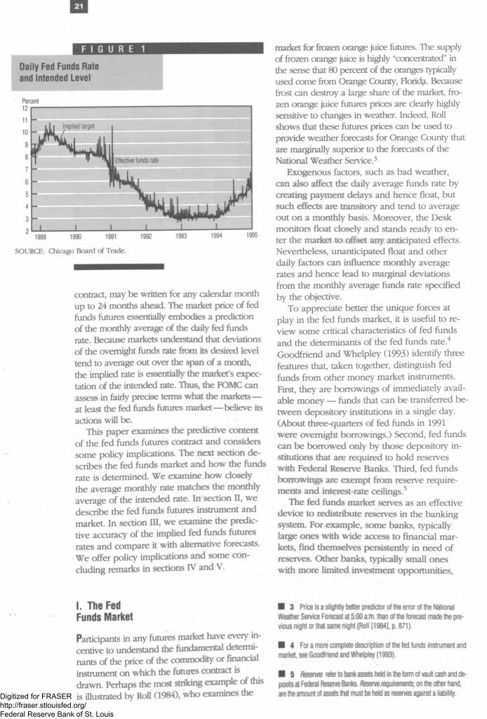
21

F I G U R E 1

Daily Fed Funds Rate and Intended Level

Percent

SOURCE: Chicago Board of Trade.

contract, may be written for any calendar month up to 24 months ahead. The market price of fed funds futures essentially embodies a prediction of the monthly average o f the daily fed funds rate. Because markets understand that deviations of the overnight funds rate from its desired level tend to average out over the span of a month, the implied rate is essentially the market’s expectation of the intended rate. Thus, the FOMC can assess in fairly precise terms what the markets— at least the fed funds futures market— believe its actions will be.

This paper examines the predictive content o f the fed funds futures contract and considers some policy implications. The next section describes the fed funds market and how the funds rate is determined. We examine how closely the average monthly rate matches the monthly average o f the intended rate. In sectron II, we describe the fed funds futures instrument and market. In section III, we examine the predictive accuracy of the implied fed funds futures rates and compare it with alternative forecasts. We offer policy implications and some concluding remarks in sections IV and V.

I. The Fed Funds Market

Participants in any futures market have every incentive to understand the fundamental determinants of the price of the commodity or financial instrument on which the futures contract is drawn. Perhaps the most striking example of this is illustrated by Roll (1984), who examines the

market for frozen orange juice futures. The supply of frozen orange juice is highly “concentrated” in the sense that 80 percent of the oranges typically used come from Orange County, Florida. Because frost can destroy a large share of the market, frozen orange juice futures prices are clearly highly sensitive to changes in weather. Indeed, Roll shows that these futures prices can be used to provide weather forecasts for Orange County that are marginally superior to the forecasts of the National Weather Service.3

Exogenous factors, such as bad weather, can also affect the daily average funds rate by creating payment delays and hence float, but such effects are transitory and tend to average out on a monthly basis. Moreover, the Desk monitors float closely and stands ready to enter the market to offset any anticipated effects. Nevertheless, unanticipated float and other daily factors can influence monthly average rates and hence lead to marginal deviations from the monthly average funds rate specified by the objective.

To appreciate better the unique forces at play in the fed funds market, it is useful to review some critical characteristics of fed funds and the determinants of the fed funds rate.4 Goodfriend and Whelpley (1993) identify three features that, taken together, distinguish fed funds from other money market instruments. First, they are borrowings o f immediately available money — funds that can be transferred b etween depository institutions in a single day. (About three-quarters o f fed funds in 1991 were overnight borrowings.) Second, fed funds can be borrowed only by those depository institutions that are required to hold reserves with Federal Reserve Banks. Third, fed funds borrowings are exempt from reserve requirements and interest-rate ceilings.5

The fed funds market serves as an effective device to redistribute reserves in the banking system. For example, some banks, typically large ones with wide access to financial markets, find themselves persistently in need o f reserves. Other banks, typically small ones with more limited investment opportunities,

■ 3 Price is a slightly better predictor of the error of the National Weather Service Forecast at 5:00 a m than of the forecast made the previous night or that same night (Roll [1984], p. 871).

■ 4 For a more complete description of the fed funds instrument and market, see Goodfriend and Whelpley (1993).

■ 5 Reserves refer to bank assets held in the form of vault cash and deposits at Federal Reserve Banks. Reserve requirements, on the other hand, are the amount of assets that must be held as reserves against a liability.Digitized for FRASER


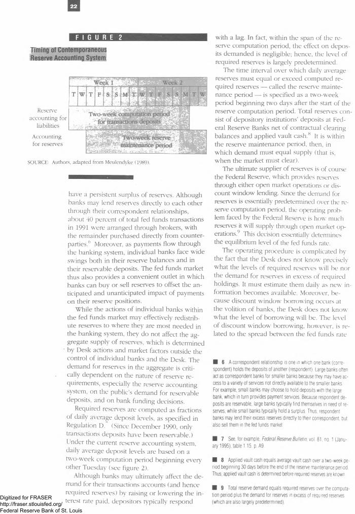
22

F I G U R E 2

Timing of Contemporaneous Reserve Accounting System

Reserve accounting for

liabilities

A ccounting for reserves

SOURCE: Authors, adapted from Meulendyke (1989).

have a persistent surplus o f reserves. Although banks may lend reserves directly to each other through their correspondent relationships, about 40 percent o f total fed funds transactions in 1991 were arranged through brokers, with the remainder purchased directly from counterparties.6 Moreover, as payments flow through the banking system, individual banks face wide swings both in their reserve balances and in their reservable deposits. The fed funds market thus also provides a convenient outlet in which banks can buy or sell reserves to offset the anticipated and unanticipated impact o f payments on their reserve positions.

While the actions o f individual banks within the fed funds market may effectively redistribute reserves to where they are most needed in the banking system, they do not affect the aggregate supply o f reserves, which is determined by Desk actions and market factors outside the control of individual banks and the Desk. The demand for reserves in the aggregate is critically dependent on the nature of reserve requirements, especially the reserve accounting system, on the public’s demand for reservable deposits, and on bank funding decisions.

Required reserves are computed as fractions o f daily average deposit levels, as specified in Regulation D. (Since December 1990, only transactions deposits have been reservable.) Under the current reserve accounting system, daily average deposit levels are based on a two-week computation period beginning every' other Tuesday (see figure 2).

Although banks may ultimately affect the demand for their transactions accounts (and hence required reserves) by raising or lowering the interest rate paid, depositors typically respond

with a lag. In fact, within the span of the reserve computation period, the effect on deposits demanded is negligible; hence, the level of required reserves is largely predetermined.

The time interval over which daily average reserves must equal or exceed computed required reserves — called the reserve maintenance period — is specified as a two-week period beginning two days after the start of the reserve computation period. Total reserves consist o f depository institutions’ deposits at Federal Reserve Banks net o f contractual clearing balances and applied vault cash .8 It is within the reserve maintenance period, then, in which demand must equal supply (that is, when the market must clear).

The ultimate supplier of reserves is of course the Federal Reserve, which provides reserves through either open market operations or discount window lending. Since the demand for reserves is essentially predetermined over the reserve computation period, the operating problem faced by the Federal Reserv e is how much reserves it will supply through open market operations.9 This decision essentially determines the equilibrium level of the fed funds rate.

The operating procedure is complicated by the fact that the Desk does not know precisely what the levels of required reserves will be nor the demand for reserves in excess of required holdings. It must estimate them daily as new information becom es available. Moreover, because discount window borrowing occurs at the volition of banks, the Desk does not know what the level o f borrowing will be. The level o f discount window borrowing, however, is related to the spread between the fed funds rate

■ 6 A correspondent relationship is one in which one bank (correspondent) holds the deposits of another (respondent). Large banks often act as correspondent banks tor smaller banks because they may have access to a variety of services not directly available to the smaller banks.For example, small banks may choose to hold deposits with the large bank, which in turn provides payment services. Because respondent deposits are reservable, large banks typically find themselves in need of reserves, while small banks typically hold a surplus. Thus, respondent banks may lend their excess reserves directly to their correspondent, but also sell them in the fed funds market

■ 7 See, for example, Federal Reserve Bulletin, vol. 81, no. 1 (January 1995), table 1.15, p.A9.

■ 8 Applied vault cash equals average vault cash over a two-week period beginning 30 days before the end of the reserve maintenance period Thus, applied vault cash is determined before required reserves are known

■ 9 Total reserve demand equals required reserves over the computation period plus the demand for reserves in excess of required reserves (which are also largely predetermined)


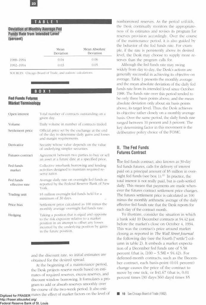
23

T A B L E 1

Deviation of Monthly Average Fe Funds Rate from Intended Level (percent)

MeanDeviation

Mean Absolute Deviation

1988-19941992-1994

0.04

0.03

0.06

0.05

SOURCES: Chicago Board of Trade; and authors' calculations.

B 0 X 1

Fed Funds Futures Market Terminology

Open interest Total number of contracts outstanding on agiven day.

Volume Daily volume in number of contracts traded.

Settlement price Official price set by the exchange at the end of the day to determine daily gains and losses and margin requirements.

Derivative Security whose value depends on the valueof underlying simpler securities.

Futures contract Agreement between two parties to buy or sell an asset at a future date at a specified price.

Fed funds Collective interbank borrowing and lendingmarket activities designed to maintain required re

serve ratios.

Fed funds Average daily rate on overnight fed funds aseffective rate reported by the Federal Reserve Bank of New

York.

Trading unit S5 million overnight fed funds held for aminimum of 30 days.

Price bias Settlement price calculated as 100 minus themonthly average overnight fed funds rate.

Hedging Taking a position that is equal and oppositeto the risk exposure relative to a market position in an attempt to offset any losses incurred by the underlying position by gains in the future position.

and the discount rate, so initial estimates are obtained for the desired spread.

At the beginning o f a maintenance period, the Desk projects reserve needs based on estimates of required reserves, excess reserves, and discount window borrowing. It formulates a program to add or absorb reserves smoothly over the course of the two-week period. It also estimates the effect of market factors on the level of

nonborrowed reserves. As the period unfolds, the Desk continually monitors the appropriateness of its estimates and revises its program for reserves provision accordingly. Over the course of the maintenance period, it is also guided by the behavior of the fed funds rate. For example, if the rate is persistently above its desired level, the Desk may choose to supply more reserves than the program calls for.

Although the fed funds rate may swing widely from day to day, the Desk’s actions are generally successful in achieving its objective on average. Table 1 presents the monthly average and the mean absolute deviation of the daily fed funds rate from its intended level since October 1988. The funds rate over this period tended to be only three basis points above, and the mean absolute deviation only about six basis points above, its target level. Thus, the Desk achieves its objective rather closely on a monthly average basis. Over the same period, the daily funds rate ranged between 10 percent and 3 percent. The key determining factor in this movement is the deliberative policy choice of the FOMC.

II. The Fed Funds Futures Contract

The fed funds contract, also known as 30-day fed funds futures, calls for delivery of interest paid on a principal amount of $5 million in overnight fed funds (see box l ).10 In practice, the total interest is not really paid, but is cash-settled daily. This means that payments are made whenever the futures contract settlement price changes. The futures settlement price is calculated as 100 minus the monthly arithmetic average of the daily effective fed funds rate that the Desk reports for each day of the contract month.

To illustrate, consider the situation in which a bank sold 10 December contracts at 94.42 just before the market’s close on O ctober 4, 1994. This was the contract’s price around market closing as reported in The Wall Street Journal the following day (see the fourth [“settle”] column in table 2). It embeds a market expectation of a Decem ber fed funds rate of 5.58 percent (that is, [100 - 5.58] = 94.42). For deferred-month contracts, such as the D ecem ber contract, each basis-point (0.01 percent) change causes the price of the contract to move by one tick, or $41.67 (that is, 0.01 percent times [30 days/360 days] times $5

10 See Chicago Board of Trade (1992).Digitized for FRASER http://fraser.stlouisfed.org/ Federal Reserve Bank of St. Louis

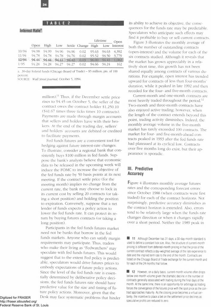
24

T A B L E 2

Interest Ratea

Lifetime OpenOpen High Low Settle Change High Low Interest

10/94 94.98 94.99 94.96 94.96 0.02 95.63 94.63 4,39211/94 94.78 94.78 94.78 94.76 0.02 95.52 94.50 3,77912/94 94.44 94.44 94.41 94.42 0-03 96,00 94.41 1,0821/95 94.28 94.28 94.27" 94.27 0.02 94.66 94.24 162

a. 30-day federal funds (Chicago Board of Trade) - $5 million; pts. of 100 percent.SOURCE. Wall Street Journal, October 5, 1994.

m illion).11 Thus, if the D ecem ber settle price rises to 94.45 on O ctober 5, the seller o f the contract ow es the contract holder $1,250.10 ($41.67 times three ticks times 10 contracts). Payments are made through margin accounts that sellers and holders have with their brokers. At the end of the trading day, sellers’ and holders' accounts are debited or credited to facilitate payments.

Fed funds futures are a convenient tool for hedging against future interest-rate changes.To illustrate, consider a regional bank that consistently buys $100 million in fed funds. Suppose the bank’s analysts believe that econom ic data to be released in the upcoming week will induce the FOMC to increase the objective of the fed funds rate by 50 basis points at its next meeting. If the contract settle price (for the meeting month) implies no change from the current rate, the bank may choose to lock in its current cost by selling 20 contracts (or taking a short position) and holding the position to expiration. Conversely, suppose that a net lender o f funds expects a policy action to lower the fed funds rate. It can protect its return by buying futures contracts (or taking a long position).

Participants in the fed funds futures market need not be banks that borrow in the fed funds markets. Anyone who can satisfy margin requirements may participate. Thus, traders who make their living as “Fedwatchers” may speculate with fed funds futures. This would suggest that to the extent Fed policy is predictable, speculators would drive futures prices to embody expectations o f future policy actions. Since the level o f the fed funds rate is essentially determined by deliberative policy decisions, the fed funds futures rate should have predictive value for the size and timing o f future policy actions. Moreover, given that the Desk may face systematic problems that hinder

its ability to achieve its objective, the consequences for the funds rate may be predictable. Speculators who anticipate such effects may find it profitable to buy or sell current contracts.

Figure 3 illustrates the monthly average of both the number of outstanding contracts (open-interest) and the volume for each of the six contracts studied. Although it reveals that the market has grown appreciably in a relatively short time, this growth has not been shared equally among contracts o f various durations. For example, open interest has trended upward for contracts o f less than four-months’ duration, while it peaked in late 1992 and then receded for the four- and five-month contracts.

Current-month and one-month contracts are most heavily traded throughout the period.12 Two-month and three-month contracts have also enjoyed active trading; however, when the length o f the contract extends beyond this point, trading activity diminishes. Indeed, the monthly average volume in the five-month market has rarely exceeded 100 contracts. The market for four- and five-month-ahead contracts peaked in 1993 after the fed funds rate had plateaued at its cyclical low. Contracts over five months long do exist, but their appearance is sporadic.

III. Predictive Accuracy

Figure 4 illustrates monthly average futures rates and the corresponding forecast errors since October 1988 (when contracts were first traded) for each of the contract horizons. Not surprisingly, predictive accuracy diminishes as the contract horizon is extended. Also, errors tend to be relatively large when the funds rate changes direction or when it changes rapidly over a short period. Neither the 1989 peak in

B 11 Although December has 31 days, a 30-day-month standard is used to define a constant tick size. Also, the structure of current-month pricing is different from deferred-month pricing in that the price of the current contract reflects a day-weighted average of the rate experience to date and the implied term rate to the end of the month. Contracts are listed on the Chicago Board of Trade exchange for the current month and for each of the 24 months that follow.

■ 12 However, on a daily basis, current-month volume often drops below one-month volume given the dramatic decline in the number of contracts generally associated with trading during the final days of the month. At the same time, there is an opportunity for arbitrage as trading forces the convergence of the futures price with the spot price as the contract approaches maturity. As the closing price becomes a virtual certainty, the incentive to place a bet on the settlement price declines as speculative profits are reduced to zero.


25

F I G U R E 3

Size of Market

Number of contracts Number of contracts


SOURCE: Chicago Board of Trade.




the funds rate nor the policy turnaround in February 1994 was anticipated at any contract horizon. Nor did the market adequately foresee the sequence o f funds-rate reductions initiated in mid-1990 and again in 1991.

That the fed funds futures market failed to anticipate these episodes may not be all that damning. Because such decisions are often based on information that surprises both forecasters and policymakers alike, there may be no way to predict the timing of such events. Moreover, the market may b e dominated by hedgers, who seek to reduce risk rather than to speculate on a projected change. The uncer

tainty surrounding the response of policy may be too great for some speculators to act on the projection. That is, the expected rate of return may not be sufficient to compensate for the level o f risk to which the position is exposed.

One might expect that the current month’s futures rate would be a good predictor of the month’s fed funds rate. Alter all, by the middle of the month, the market already knows half of the daily rates used in the monthly average calculation. Moreover, as time moves on, more information relevant to policy decisions becomes available, which in turn should enhance the predictive performance of a given contract. For example, oneDigitized for FRASER


26

F I G U R E 4

Fed Funds Futures Rate as a Predictor of the Effective Fed Funds Rate

Percent Percent Percent Percent

Percent Percent

a. Line breaks reflect periods during which no contracts were traded.SOURCES: Chicago Board of Trade; and Board of Governors of the Federal Reserve System.

would exp ea the probability of an unanticipated shift in Fed policy to diminish as the expiration date of a contract approaches.

To examine how readily the futures market incorporates available information into its pricing decisions, we estimate the mean absolute deviation between the daily rate and the contract standard for each of the trading days leading up to the expiration date. In principle, if the market is efficient, the mean absolute deviation should diminish. Figure 5 illustrates that the deviation declines steadily as the expiration

date approaches. Indeed, the mean absolute deviation is virtually zero by the last trading day. Moreover, the mean absolute deviation averaged over the month is less than six basis points, about the same as the mean absolute deviation of the fed funds rate from its monthly average intended rate. This suggests that all systematic variation in the fed funds rate is anticipated by the market and incorporated into the future’s price. If the fed funds futures market were not incorporating all the information about future fed funds yields, one might expect


27

F I G U R E 5

Mean Absolute Deviation of Future from Effective Funds Rate

Basis points

Trading days remaining in calendar month

SOURCES: Chicago Board of Trade; and authors' calculations.

B 0 X 2

Alternative Forecasting Models

Naive Model (random walk)

where r t is the effective fed funds rate and £, is a random

disturbance.

Univariate Model (estimated)

A rt = 0.011 + 0.367 A r(. , + e,(0.046) (7.912)

where A rt is the first difference of the effective fed funds rate and e, is an independent, identically distributed (i.i.d.) random disturbance. The equation is estimated from September 1954 to September 1988.

that the mean absolute deviation of the futures rate would materially exceed that of the fed funds rate from its intended level.13

Market participants are clearly able to improve their estimates of the current month’s average as the month progresses. What's more impressive is that the predictive accuracy of the one-month-ahead futures rate also improves over the period leading up to the end o f the prior month. The mean absolute error on the last day o f the previous month is about

one-third lower than the mean absolute error 20 days earlier. The only exception to this trend occurs for a few days in the middle of a calendar month. Nevertheless, the predictive performance is not significantly diminished.

To the extent that the fed funds futures market is efficient, contract rates should predict fed funds rates at least as well as alternative forecasting models. As a preliminary investigation of market efficiency, we compare the prediction errors of fed funds futures with those of a naive model and an estimated univariate model (first-order autoregressive model of the change in the fed funds rate).14 The naive model simply assumes that the best forecast of the future fed funds rate is the current rate (see box 2). This model is sometimes called a random walk because it implicitly assumes that changes to the fed funds rate are random and permanent. The univariate model also assumes that changes to the level of the fed funds rate are permanent, but it allows for some persistence of the change. That is, if a change occurs in one period, it can occur again (at least partially) in the subsequent period.

Table 3 presents the mean prediction error (MPE) and the mean square error (MSE) for each of six forecast horizons and for each of the alternative forecasting approaches.15 The prediction error is defined as the forecast less the actual (monthly average effective fed funds rate). All three approaches tended to overpredict over the whole period. The bias was uniformly larger for predictions based on fed funds futures rates, the only exception being for the five-month-ahead horizon. This suggests that fed funds futures pricing may be dominated by consistent borrowers of overnight funds who are willing to pay a premium to hedge against the risk of interest-rate increases.16 Given the limited sample, however, it may be too early to draw such a conclusion.17

■ 13 Both measures of variability are small.

■ 14 This model, an ARIMA (1,1,0), was identified using a method proposed by Box and Jenkins (1970).

■ 15 The /'-month-ahead prediction errors for the futures contract are simply the difference between the futures rate on the /-month-ahead contract and the average of the fed funds rate for the same month. All contract rates are averaged over the month that they are recorded.

■ 16 One might ask why this premium exists. It is possible that transactions costs may preclude any profitable strategy to exploit the premium.

■ 17 Indeed, Spence Hilton at the Trading Desk of the Federal Reserve Bank of New York believes that the prediction bias may be a quirk of the sample period. He notes that over most of the sample period, the market (as well as the F0MC) was surprised by the lack of strength in the economy. The F0MC often responded to evidence of economic weakness by lowering the fed funds rate immediately. He believes that this experience could dominate the average prediction error given the limited sample.


28

T A B L E 3

Relative Predictive Accuracy of Fed Funds Futures

Panel A. W hole Forecast Period (O cto b er 1 9 8 8 -D e ce m b e r 19 9 4 )

Federal Funds Futures Naive Model Univariate Model

Forecast Horizon MPEa MSEb MPE MSE MPE MSE

Current 0.01 0.00 — — — —One month ahead 0.06 0.03 0.04 0.05 0.03 0.04Two months ahead 0.10 0.09 0.08 0.17 0.08 0.13Three months ahead 0.17 0.20 0.14 0.33 0.15 0.27Four months ahead 0.25 0.36 0.20 0.54 0.22 0.48Five months ahead 0.26 1.62 0.27 0.77 0.30 0.72

Panel B. Second Half o f Forecast Period (after 1 9 9 1 )

Federal Funds Futures Naive Model Univariate Model

Forecast Horizon MPEa MSEb MPE MSE MPE MSE

Current 0.01 0.01 — — — —One month ahead 0.06 0.03 -0 .0 4 0.04 -0 .0 1 0.03Two months ahead 0.10 0.06 -0 .0 7 0.12 -0 .0 2 0.09Three months ahead 0.13 0.11 -0 .0 6 0.22 -0 .0 0 0.16Four months ahead 0.18 0.18 -0 .0 5 0.38 0.03 0.31Five months ahead 0.23 0.29 -0 .2 2 0.75 0.08 0.49

a. Mean prediction error.b. Mean square error.SOURCE: Authors' calculations.

Although alternative models may provide less-biased predictions than the fed funds futures, investment strategies based on the models would be more risky. This is evident when comparing the MSEs of alternative forecasts. The MSE provides a measure o f the dispersion o f forecast errors and hence o f the uncertainty associated with the prediction. In all but one case, the MSE o f the fed funds futures prediction is less than the alternatives.18 Thus, although the average gain could be greater for alternative predictions, the potential for losses is also higher.

Because the fed funds futures market is young and the volume of trades is small relative to some other comparable instruments (for example, Eurodollar futures), one might question whether the market is “deep” enough to accommodate large trades. If the market is deep, large trades should not appreciably affect market rates unless they reflect the incorporation of new information in futures prices. To assess the potential relevance of this issue, we examine whether the increased volume of the market has led to better predictions. The second panel in table 3 presents the MPE and MSE statistics for the period since 1991. These results reveal that the

dispersion of forecast errors declines sharply for horizons o f three months or more. However, the improved predictive performance over the latter period may reflect the fact that the fed funds rate was relatively more stable over this period.

In sum, the preliminary' evidence presented above suggests that fed funds futures are useful for predicting future fed funds rate changes (and hence policy moves), especially over the shorter forecast horizons. Prediction error is shown to diminish almost daily leading up to a contract’s expiration date. The fact that the MSEs o f fed funds futures predictions are relatively small provides some evidence that fed funds futures markets efficiently incorporate information into pricing decisions.

■ 18 The only exception is lor the five-month-ahead futures contract, which was not actively traded over the first three years of the market


29

IV. Some Policy Implications

The fed funds futures rate, by virtue of being a market-determined expectation about future deliberative actions, provides potentially useful in- fonnation for Fed policymakers. For example, the FOMC may find the futures rate helpful in assessing the credibility of alternative policy choices. To illustrate, consider a situation in which financial markets clearly perceive increasing inflationary pressures and exp ea the FOMC to counter with a fed funds rate increase.

A key market concern may be that the FOMC must demonstrate sufficient resolve to ensure that short-term objectives — such as interest-rate smoothing — do not interfere with the achievement of longer-tenn price stability. Under these circumstances, the absence of an anticipated action could induce expectations of rising inflation and in turn become embedded in longer-term interest rates as increased inflation premia. Thus, if the market expects an anti-inflationary move, the FOMC may feel compelled to act even if it believes inflationary pressure will ebb so as to prevent a flare-up of inflationary expectations.

To what extent should the FOMC react to fed funds futures as a signal of expectations regarding future changes? In principle, participants in the fed funds futures market will base their trading decisions on expectations of the fed funds rate path they believe the FOMC will choose over time. If the FOMC were to base its decision solely on the market’s expectation, it is not clear what would ultimately determine the fed funds rate path. That is, the equilibrium outcome of such a policy may be indetenninate. This problem is described by Keynes (1936, p. 156) in an analogy with newspaper competitions:

... the competitors have to pick out the six prettiest faces from a hundred photographs, the prize being awarded to the competitor w hose choice most nearly corresponds to the average preferences of the competitors as a whole; so that each competitor has to pick, not those faces which he himself finds prettiest, but those which he thinks likeliest to catch the fancy of other competitors, all of whom are lcx)king at the problem from the same point of view . It is not the case of choosing those which, to the best of one’s judgment, are really the prettiest, nor even those which average opinion genuinely thinks is the prettiest. We have reached the third degree where we devote our intelligences to anticipating what average opinion expects average opinion to be. And there are soriK*. I believe, who practise the fourth, fifth and higher degrees.

One cannot know at which degree participants choose to make their decision; hence the indeterminacy.

The FOMC, o f course, does not base its decision solely on what the market expects it to do, as clearly evidenced by the failure of the fed funds futures market to anticipate turning points in fed funds rates. Rather, the FOMC looks at many things, and bases its decision on the majority’s assessment of the fed funds rate level needed to accomplish ultimate objectives. In this context, however, the Committee may find knowledge of market expectations useful in assessing the financial-market consequences of alternative actions. For example, the estimated impact of any given action may differ depending on whether the policy change is anticipated by the market. Thus, fed funds futures rates are helpful as part of an array of indicators considered by the FOMC in its policy deliberations.

V. Concluding Remarks

Futures contracts are typically drawn on com modities or financial instruments whose price or yield is determined in competitive markets. In the case of fed funds, however, the rate is essentially determined by a deliberative decision of the FOMC, the main policymaking arm of the Federal Reserve System. Hence, the fed funds futures market must anticipate actions taken by the FOMC. In short, through the fed funds futures market, one can place a bet on what future monetary policy will be. The Committee then can get a clear reading of what these market participants expect them to do, which may at times be helpful for FOMC members who place great weight on knowing if a policy choice would surprise the market.

If they are to be instructive for policymakers, fed funds futures rates should have some predictive content. The predictive accuracy of futures rates clearly improves over the two-month period leading up to the contract’s expiration, providing some evidence that the market is efficient in incorporating new information into its pricing. The largest prediction errors occur around policy turning points. Nevertheless, the evidence above suggests that the fed funds futures markets are efficient processors of information concerning the future path of the fed funds rate.


30

References

Chicago Board of Trade. 30-Day Fed Funds Futures-. Flexible Futures fo r Managing Risk. Chicago: Board o f Trade of the City of Chicago, 1992.

Box, George E.P., and Gwilym M. Jenkins. Time Series Analysis: Forecasting an d Control. San Francisco: Holden-Day, 1970.

Goodfriend, Marvin, and William Whelpley.“Federal Funds,” in Timothy Q. Cook and Robert K. LaRoche, eds., Instruments o f the Money Market. Richmond: Federal Reserve Bank of Richmond, 1993, pp. 8 - 2 1 .

Keynes, John Maynard. The General Theory o f Employment, Interest, an d Money. New York: Harcourt, Brace, and World, 1936.

Meulendyke, Ann-Marie. U.S. Monetary Policy an d Financial Markets. New York: Federal Reserve Bank of New York, 1989.

Roll, Richard. “Orange Juice and W eather,” American Economic Review, vol. 74, no. 5 (Decem ber 1984), pp. 8 6 1 -8 0 .


31

First Quarter Working Papers

Institutional subscribers, such as libraries and other organizations, will be placed on a mailing list upon request and will automatically receive Working Papers as they are published.

Current Working Papers of the Cleveland Federal Reserve Bank are listed in each quarterly issue of the Economic Review. Copies of specific papers may be requested by completing and mailing the attached form below.

Single copies of individual papers will be sent free of charge to those who request them. A mailing list service for personal subscribers, however, is not available.

■ 9417Bank Diversification: Laws and Fallacies of Large Numbersby Joseph G. Haubrich

■ 9418The Effects of Inflation on Wage Adjustments in Firm-Level Data: Grease or Sand?by Erica L. Groshen and Mark E. Schweitzer

■ 9419Posted Rates as Signals in Mortgage Lending Marketsby Robert B. Avery, Patricia E. Beeson, and Mark S. Sniderman

■ 9420The Computational Experiment:An Econometric Toolby Finn E. Kydland and Edward C. Prescott

■ 9421Underserved Mortgage Markets: Evidence from HMDA Databy Robert B. Avery, Patricia E. Beeson, and Mark S. Sniderman

■ 9501More on the Differences between Reported and Actual U.S. Central Bank Foreign Exchange Interventionby William P. Osterberg and Rebecca Wetmore Humes

Please complete and detach the form below and mail to:Research DepartmentFederal Reserve Bank of ClevelandP.O. Box 6387Cleveland, Ohio 44101

Check item(s) requested

Send to:Please print

Please send the following Working Paper(s):

□ 9417 □ 9419 □ 9421□ 9418 □ 9420 □ 9501

Name

Address

City State ZipDigitized for FRASER http://fraser.stlouisfed.org/ Federal Reserve Bank of St. Louis

32

The Federal Reserve Bank of Cleveland and the Journal of Money, Credit and Banking

Announce:

Derivatives and IntermediationNovember 2-3,1995 Cleveland, Ohio

The Federal Reserve Bank of Cleveland and the Journal of Money, Credit and Banking are jointly sponsoring a conference on Derivatives and Intermediation:Theory and Evidence.

The growing derivatives market poses several challenges for policymakers. The first is to understand the sources of financial innovation resulting in the proliferation of these products. What economic forces make derivatives viable instruments? What gains do rational participants obtain from these contracts, and why do they dominate transactions in the cash securities markets? To what extent does regulatory policy— bankruptcy rules, capital requirements, accounting rules, and deposit insurance— affect the market? In other words, does derivative- related financial innovation stem from changes in the marketplace, or from changes in the regulatory environment? The answer is crucial to understanding both derivatives and intermediation. The second challenge for policymakers is to understand how derivatives impact regulatory concerns in the areas of bank risk, payments system reform, and intermediary powers.

Call for PapersThe conference proceedings will be published in the Journal of Money, Credit and Banking, and authors will receive an honorarium. Prospective contributors are invited to send a completed paper or detailed abstract by May 30,1995 to:

Joseph G. Haubrich Research Department Federal Reserve Bank of Cleveland P.O. Box 6387 Cleveland, OH 44101-1387


economic review - fraser

Documents