economics 102 lecture 10 market equilibrium rev
TRANSCRIPT

7/27/2019 Economics 102 Lecture 10 Market Equilibrium Rev
http://slidepdf.com/reader/full/economics-102-lecture-10-market-equilibrium-rev 1/62
8/3/200
Lecture 10: Equilibrium
Introduction
Market equilibrium
Comparative statics
The effects of taxes
Pareto efficiency

7/27/2019 Economics 102 Lecture 10 Market Equilibrium Rev
http://slidepdf.com/reader/full/economics-102-lecture-10-market-equilibrium-rev 2/62
8/3/200
Supply
Supply curve – measures how much a firm is
willing to supply of a good at each possible
market price, i.e., for each p, how much of
the good S(p) will be supplied
Market supply curve –it is just the sum of the
individual supply curves of suppliers of thegood
Assume a competitive market
Competitive market – individual consumers and
suppliers take prices as given, and determine their best
response given those market prices.
Rationale: the consumer or supplier is small relative tothe market and thus has a negligible effect on the market
price.
It is the actions of all the agents together that determine
the market price.

7/27/2019 Economics 102 Lecture 10 Market Equilibrium Rev
http://slidepdf.com/reader/full/economics-102-lecture-10-market-equilibrium-rev 3/62
8/3/200
Equilibrium price – price at which the supplyof the goods equal the demand.
Let:
market demand curve :
market supply curve:
, the equilibrium price is the pricethat solves the equation:
)( p D
)( pS * p
)()( ** pS p D
Demand and supply curves represent theoptimal choices of the agents involved andthe fact that they are equal at some price p*means that the behaviors of demandersand suppliers are compatible.
In equilibrium, all agents are choosing thebest action for themselves and eachperson’s behavior is consistent with that of others.

7/27/2019 Economics 102 Lecture 10 Market Equilibrium Rev
http://slidepdf.com/reader/full/economics-102-lecture-10-market-equilibrium-rev 4/62
8/3/200
Only when the amount that people want to buy at agiven price equals the amount that people want to sellat that price will the market be in equilibrium
Demand is greater than supply: Some suppliers realize that they can sell at a higher price to
some of the demanders, thus prices would be pushed up.
Supply is greater than demand: some suppliers will not be able to sell at the going price and the
only way they can sell more is if they lower the price.
*' p p
*' p p
p
D(p)
q=D(p)
Marketdemand

7/27/2019 Economics 102 Lecture 10 Market Equilibrium Rev
http://slidepdf.com/reader/full/economics-102-lecture-10-market-equilibrium-rev 5/62
8/3/200
p
S(p)
Marketsupply
q=S(p)
p
D(p), S(p)
q=D(p)
Marketdemand
Marketsupply
q=S(p)

7/27/2019 Economics 102 Lecture 10 Market Equilibrium Rev
http://slidepdf.com/reader/full/economics-102-lecture-10-market-equilibrium-rev 6/62
8/3/200
p
D(p), S(p)
q=D(p)
Market
demandMarketsupply
q=S(p)
p*
q*
p
D(p), S(p)
q=D(p)
Marketdemand
Marketsupply
q=S(p)
p*
q*
D(p*) = S(p*); the marketis in equilibrium.

7/27/2019 Economics 102 Lecture 10 Market Equilibrium Rev
http://slidepdf.com/reader/full/economics-102-lecture-10-market-equilibrium-rev 7/62
8/3/200
p
D(p), S(p)
q=D(p)
Market
demandMarketsupply
q=S(p)
p*
S(p’)
D(p’) < S(p’); an excess
of quantity supplied over quantity demanded.
p’
D(p’)
p
D(p), S(p)
q=D(p)
Marketdemand
Marketsupply
q=S(p)
p*
S(p’)
D(p’) < S(p’); an excess
of quantity supplied over quantity demanded.
p’
D(p’)
Market price must fall towards p*.
7/27/2019 Economics 102 Lecture 10 Market Equilibrium Rev
http://slidepdf.com/reader/full/economics-102-lecture-10-market-equilibrium-rev 8/62
8/3/200
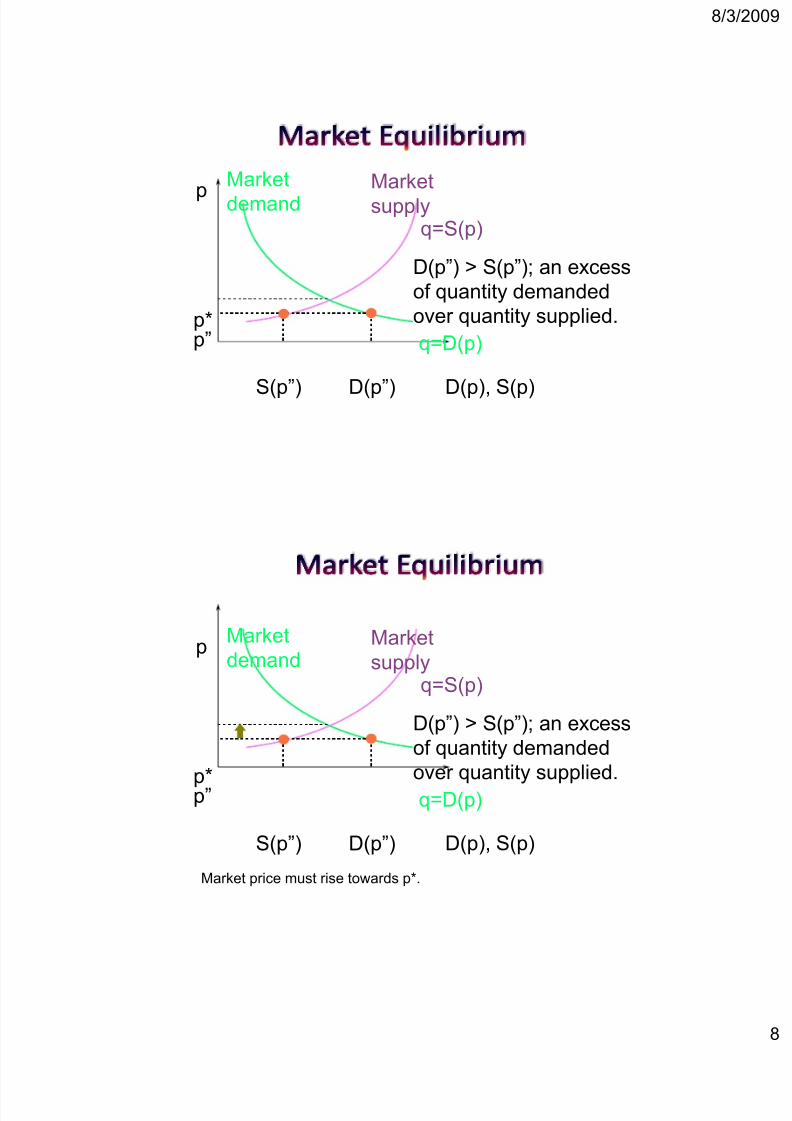
p
D(p), S(p)
q=D(p)
Market
demandMarketsupply
q=S(p)
p*
D(p”)
D(p”) > S(p”); an excess
of quantity demandedover quantity supplied.
p”
S(p”)
p
D(p), S(p)
q=D(p)
Marketdemand
Marketsupply
q=S(p)
p*
D(p”)
D(p”) > S(p”); an excess
of quantity demandedover quantity supplied.
p”
S(p”)
Market price must rise towards p*.

7/27/2019 Economics 102 Lecture 10 Market Equilibrium Rev
http://slidepdf.com/reader/full/economics-102-lecture-10-market-equilibrium-rev 9/62
8/3/200
An example of calculating a market
equilibrium when the market demand and
supply curves are linear.
D p a bp( )
S p c dp( )
p
D(p), S(p)
D(p) = a-bp
Marketdemand
Marketsupply
S(p) = c+dp
p*
q*

7/27/2019 Economics 102 Lecture 10 Market Equilibrium Rev
http://slidepdf.com/reader/full/economics-102-lecture-10-market-equilibrium-rev 10/62
8/3/200
1
p
D(p), S(p)
D(p) = a-bp
Market
demandMarketsupply
S(p) = c+dp
p*
q*
What are the valuesof p* and q*?
D p a bp( )
S p c dp( )
At the equilibrium price p*, D(p*) = S(p*).That is,
a bp c dp * *
which givesp a c
b d
*
andq D p S p
ad bc
b d
* * *( ) ( ) .

7/27/2019 Economics 102 Lecture 10 Market Equilibrium Rev
http://slidepdf.com/reader/full/economics-102-lecture-10-market-equilibrium-rev 11/62
8/3/200
p
D(p), S(p)
D(p) = a-bp
Market
demandMarketsupply
S(p) = c+dp
p
a c
b d
*
dbbcadq*
Equilibrium via inverse demand and supply
curves
Inverse demand – price that someone is willing
to pay in order to acquire some given amount of the good
Inverse supply – price that must prevail in order
to generate a given amount of supply

7/27/2019 Economics 102 Lecture 10 Market Equilibrium Rev
http://slidepdf.com/reader/full/economics-102-lecture-10-market-equilibrium-rev 12/62
8/3/200
1
Equilibrium price - determined by finding that
quantity at which the amount the demanders are
willing to pay to consume that quantity is equal to
the price that suppliers must receive in order to
supply that quantity.
inverse supply:
inverse demand:
equilibrium is determined by the condition:
)( *q P S
)( *q P D
)()( ** q P q P DS
q D p a bp pa q
bD q
( ) ( ),1
q S p c dp pc q
d
S q
( ) ( ),1
the equation of the inverse marketdemand curve. And
the equation of the inverse marketsupply curve.

7/27/2019 Economics 102 Lecture 10 Market Equilibrium Rev
http://slidepdf.com/reader/full/economics-102-lecture-10-market-equilibrium-rev 13/62
8/3/200
1
q
D-1(q),S-1(q)
D-1(q) = (a-q)/b
Market
inversedemand
Market inverse supplyS-1(q) = (-c+q)/d
p*
q*
q
D-1(q),S-1(q)
D-1(q) = (a-q)/b
Marketdemand
S-1(q) = (-c+q)/d
p*
q*
At equilibrium,D-1(q*) = S-1(q*).
Market inverse supply

7/27/2019 Economics 102 Lecture 10 Market Equilibrium Rev
http://slidepdf.com/reader/full/economics-102-lecture-10-market-equilibrium-rev 14/62
8/3/200
1
p D qa q
b
1( ) p S q
c q
d
1( ) .and
At the equilibrium quantity q*, D-1(p*) = S-1(p*). That is,
d
qc
b
qa **
which gives qad bc
b d
*
and p D q S q a cb d
* * *( ) ( ) .
1 1
q
D-1(q),S-1(q)
D-1(q) = (a-q)/b
Marketdemand
Marketsupply
S-1(q) = (-c+q)/d
p
a c
b d
*
db
bcadq*

7/27/2019 Economics 102 Lecture 10 Market Equilibrium Rev
http://slidepdf.com/reader/full/economics-102-lecture-10-market-equilibrium-rev 15/62
8/3/200
1
In the general case, the equilibrium price
and equilibrium quantity are jointly
determined by demand and supply curves.
Special cases
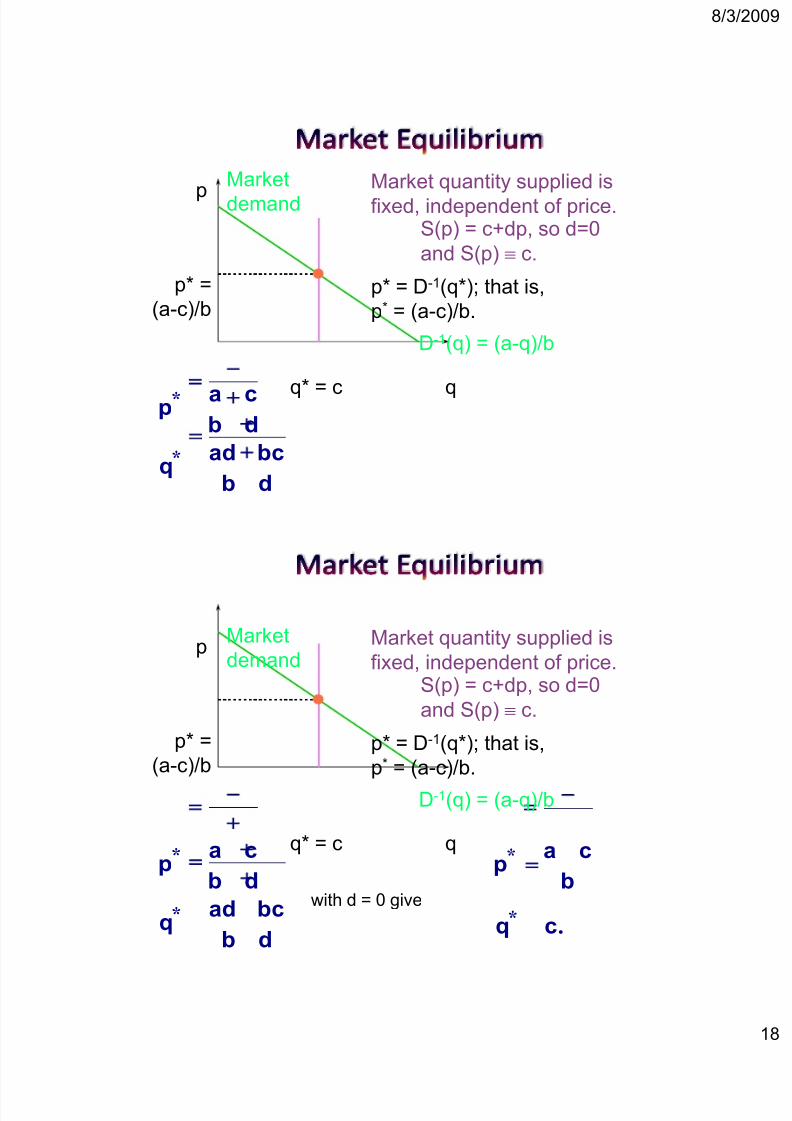
Case of the fixed supply.
Amount supplied is some fixed number and is
independent of prices. Supply curve is vertical.
Equilibrium quantity is determined entirely by
supply conditions and the equilibrium price
by demand conditions
Market quantity supplied isfixed, independent of price.
p
qq*

7/27/2019 Economics 102 Lecture 10 Market Equilibrium Rev
http://slidepdf.com/reader/full/economics-102-lecture-10-market-equilibrium-rev 16/62
8/3/200
1
S(p) = c+dp, so d=0and S(p) c.
p
qq* = c
Market quantity supplied isfixed, independent of price.
S(p) = c+dp, so d=0and S(p) c.
p
qq* = c
D-1(q) = (a-q)/b
Marketdemand
Market quantity supplied isfixed, independent of price.

7/27/2019 Economics 102 Lecture 10 Market Equilibrium Rev
http://slidepdf.com/reader/full/economics-102-lecture-10-market-equilibrium-rev 17/62
8/3/200
1
S(p) = c+dp, so d=0and S(p) c.
p
q
p*
D-1(q) = (a-q)/b
Market
demand
q* = c
Market quantity supplied isfixed, independent of price.
S(p) = c+dp, so d=0and S(p) c.
p
q
p* =(a-c)/b
D-1(q) = (a-q)/b
Marketdemand
q* = c
p* = D-1(q*); that is,p* = (a-c)/b.
Market quantity supplied isfixed, independent of price.
7/27/2019 Economics 102 Lecture 10 Market Equilibrium Rev
http://slidepdf.com/reader/full/economics-102-lecture-10-market-equilibrium-rev 18/62
8/3/200
1
S(p) = c+dp, so d=0and S(p) c.
p
q
D-1(q) = (a-q)/b
Market
demand
q* = c
p* = D-1(q*); that is,p* = (a-c)/b.
p* =(a-c)/b
Market quantity supplied isfixed, independent of price.
p a cb d
*
qad bc
b d
*
S(p) = c+dp, so d=0and S(p) c.
p
q
D-1(q) = (a-q)/b
Marketdemand
q* = c
p* = D-1(q*); that is,p* = (a-c)/b.
pa c
b d
*
qad bc
b d
*
with d = 0 give
pa c
b
*
q c* .
p* =(a-c)/b
Market quantity supplied isfixed, independent of price.

7/27/2019 Economics 102 Lecture 10 Market Equilibrium Rev
http://slidepdf.com/reader/full/economics-102-lecture-10-market-equilibrium-rev 19/62
8/3/200
1
Case of perfectly horizontal supply curve
Industry will supply any amount of the
good at a constant price
Equilibrium price is determined by
supply conditions and the equilibrium
quantity is determined by the demand
curve.
Market quantity supplied isextremely sensitive to price.
p
q

7/27/2019 Economics 102 Lecture 10 Market Equilibrium Rev
http://slidepdf.com/reader/full/economics-102-lecture-10-market-equilibrium-rev 20/62
8/3/200
2
Market quantity supplied isextremely sensitive to price.
S-1(q) = p*.p
q
p*
Market quantity supplied isextremely sensitive to price.
S-1(q) = p*.
p
q
p*
D-1(q) = (a-q)/b
Marketdemand

7/27/2019 Economics 102 Lecture 10 Market Equilibrium Rev
http://slidepdf.com/reader/full/economics-102-lecture-10-market-equilibrium-rev 21/62
8/3/200
2
Market quantity supplied isextremely sensitive to price.
S-1(q) = p*.p
q
p*
D-1(q) = (a-q)/b
Market
demand
q*
Market quantity supplied isextremely sensitive to price.
S-1(q) = p*.
p
q
p*
D-1(q) = (a-q)/b
Marketdemand
q* =a-bp*
p* = D-1(q*) = (a-q*)/b soq* = a-bp*

7/27/2019 Economics 102 Lecture 10 Market Equilibrium Rev
http://slidepdf.com/reader/full/economics-102-lecture-10-market-equilibrium-rev 22/62
8/3/200
2
How will the equilibrium price and quantitieschange when demand and supply curveschange?
Demand increases ( decreases), equilibrium priceand quantity must increase (decrease)
Supply increases (decreases), equilibrium pricesfall (rise) and equilibrium quantity increases(decreases).
Simultaneous changes in demand and supply,results depend on the magnitudes and directions of the shifts.
p
D(p), S(p)
Marketdemand
Market supply
p*
q*

7/27/2019 Economics 102 Lecture 10 Market Equilibrium Rev
http://slidepdf.com/reader/full/economics-102-lecture-10-market-equilibrium-rev 23/62
8/3/200
2
With taxes, there are two prices of interest
that differ by the amount of the tax:
price that the demander pays (demand price)
price that the supplier gets (supply price)
Quantity taxes – tax levied per unit of quantity
bought or sold:
Ad valorem or value tax. Expressed in percentage
units:
t P P sb
sb P P )1(
If the tax is levied on sellers then it is an excise
tax.
If the tax is levied on buyers then it is a sales tax.
As far as the equilibrium price facingdemanders and suppliers is concerned, it
doesn’t really matter who is responsible for
paying the tax. It just matters that the tax must
be paid by someone.

7/27/2019 Economics 102 Lecture 10 Market Equilibrium Rev
http://slidepdf.com/reader/full/economics-102-lecture-10-market-equilibrium-rev 24/62
8/3/200
2
A tax rate t makes the price paid by buyers,
pb, higher by t from the price received by
sellers, ps.
p p tb s
Even with a tax the market must clear.
I.e. quantity demanded by buyers at price pb
must equal quantity supplied by sellers at
price ps.
D p S pb s( ) ( )

7/27/2019 Economics 102 Lecture 10 Market Equilibrium Rev
http://slidepdf.com/reader/full/economics-102-lecture-10-market-equilibrium-rev 25/62
8/3/200
2
p p tb s D p S pb s( ) ( )and
describe the market’s equilibrium. Notice theseconditions apply no matter if the tax is levied on sellersor on buyers.
Hence, a sales tax rate t has the same effect as an
excise tax rate t.
Effects of quantity taxes:
Case 1: Supplier required to pay the tax.
Amount supplied will depend on the supplyprice – the amount the supplier gets afterpaying the tax.
Amount demanded will depend on thedemand price – the amount that the demanderpays.
Amount supplier gets will be the amount that the demander pays minus the amount of thetax

7/27/2019 Economics 102 Lecture 10 Market Equilibrium Rev
http://slidepdf.com/reader/full/economics-102-lecture-10-market-equilibrium-rev 26/62
8/3/200
2
This gives us two equations:
Substituting the second equation into thefirst we have the equilibrium condition: .
Alternatively we can rearrange the secondequation to get:
To get:
t P P
P S P D
b s
sb
)()(
)()( t P S P D bb
t P P sb
)()( s s P S t P D
Case 2: Demander has to pay the tax
The amount paid by the demander minus the
tax equals the price received by the supplier:
Substituting into the demand and supply
condition results in:
This is the same equation as in the case where
the supplier pays the tax.
sb P t P
)()( t P S P D bb

7/27/2019 Economics 102 Lecture 10 Market Equilibrium Rev
http://slidepdf.com/reader/full/economics-102-lecture-10-market-equilibrium-rev 27/62
8/3/200
2
Utilizing inverse demand and supply
functions:
Equilibrium quantity is that quantity q* such that
the demand price at q* minus the tax being paid is
just equal to the supply price at q*:
If the tax is being imposed on suppliers, the
condition is that the supply price plus the amount of the tax must equal the demand price:
)()( ** q P t q P sb
t q P q P sb )()( **
Geometric representation: Using the
inverse demand and supply curves
Find the quantity where the curve
crosses the curve.
Shift the demand curve downwards by the amount of
the tax.
Alternatively, we can find the quantity where
crosses .
Simply shift the supply curve by the amount of the tax
t q P b )( *
)(*
q P s
)( *q P b
t q P s )(*
7/27/2019 Economics 102 Lecture 10 Market Equilibrium Rev
http://slidepdf.com/reader/full/economics-102-lecture-10-market-equilibrium-rev 28/62
8/3/200
2
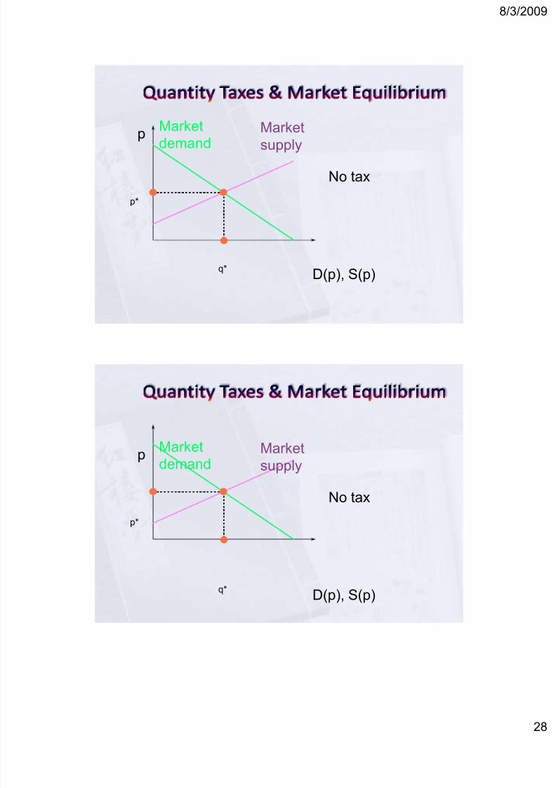
p
D(p), S(p)
Market
demandMarketsupply
p*
q*
No tax
p
D(p), S(p)
Marketdemand
Marketsupply
p*
q*
No tax
7/27/2019 Economics 102 Lecture 10 Market Equilibrium Rev
http://slidepdf.com/reader/full/economics-102-lecture-10-market-equilibrium-rev 29/62
8/3/200
2
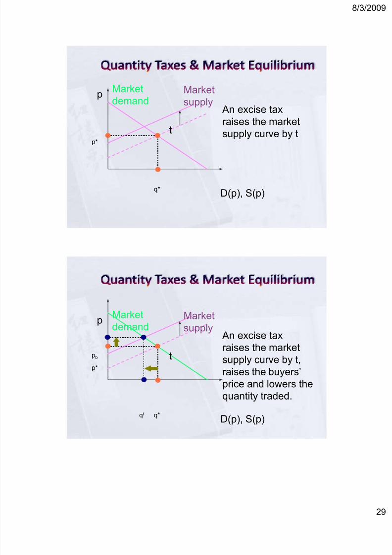
p
D(p), S(p)
Market
demandMarketsupply
p*
q*
t
An excise taxraises the marketsupply curve by t
p
D(p), S(p)
Marketdemand
Marketsupply
p*
q*
An excise taxraises the marketsupply curve by t,raises the buyers’
price and lowers thequantity traded.
tpb
qt

7/27/2019 Economics 102 Lecture 10 Market Equilibrium Rev
http://slidepdf.com/reader/full/economics-102-lecture-10-market-equilibrium-rev 30/62
8/3/200
3
p
D(p), S(p)
Market
demandMarketsupply
p*
q*
An excise taxraises the marketsupply curve by t,raises the buyers’
price and lowers thequantity traded.
tpb
qt
And sellers receive only ps = pb - t.
ps
p
D(p), S(p)
Marketdemand
Marketsupply
p*
q*
No tax

7/27/2019 Economics 102 Lecture 10 Market Equilibrium Rev
http://slidepdf.com/reader/full/economics-102-lecture-10-market-equilibrium-rev 31/62
8/3/200
3
p
D(p), S(p)
Market
demandMarketsupply
p*
q*
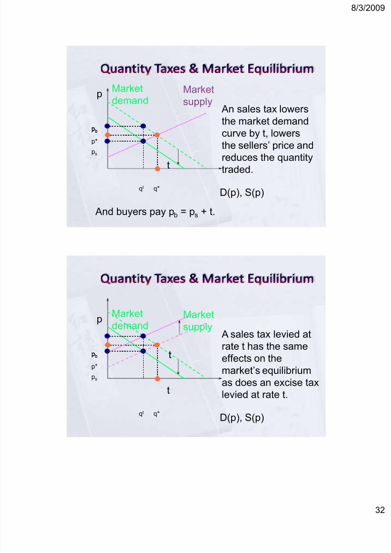
An sales tax lowersthe market demandcurve by t
t
p
D(p), S(p)
Marketdemand
Marketsupply
p*
q*
An sales tax lowersthe market demandcurve by t, lowersthe sellers’ price and
reduces the quantitytraded.t
qt
ps
7/27/2019 Economics 102 Lecture 10 Market Equilibrium Rev
http://slidepdf.com/reader/full/economics-102-lecture-10-market-equilibrium-rev 32/62
8/3/200
3
p
D(p), S(p)
Market
demandMarketsupply
p*
q*
An sales tax lowersthe market demandcurve by t, lowersthe sellers’ price and
reduces the quantitytraded.t
pbpb
qt
pb
And buyers pay pb = ps + t.
ps
p
D(p), S(p)
Marketdemand
Marketsupply
p*
q*
A sales tax levied atrate t has the sameeffects on themarket’s equilibrium
as does an excise taxlevied at rate t.t
pbpb
qt
pb
ps
t

7/27/2019 Economics 102 Lecture 10 Market Equilibrium Rev
http://slidepdf.com/reader/full/economics-102-lecture-10-market-equilibrium-rev 33/62
8/3/200
3
Another way to determine the impact of the
tax. Find the quantity q* such that when the
suppliers face ps and the demander faces
pb=ps+t, the quantity q* is demanded by
consumers and supplied by firms.
Represent the tax as a vertical segment and slide it
along the supply curve until it just touches the
demand curve.
This is the equilibrium quantity
p
D(p), S(p)
Marketdemand
Marketsupply
p*
q*
t
pbpb
qt
pb
ps

7/27/2019 Economics 102 Lecture 10 Market Equilibrium Rev
http://slidepdf.com/reader/full/economics-102-lecture-10-market-equilibrium-rev 34/62
8/3/200
3
Effects of the tax:
Quantity sold must decrease.
Price paid by demanders must go up
Price received by suppliers must go down.
E.g. suppose the market demand and supply
curves are linear.
D p a bpb b( )
S p c dps s( )

7/27/2019 Economics 102 Lecture 10 Market Equilibrium Rev
http://slidepdf.com/reader/full/economics-102-lecture-10-market-equilibrium-rev 35/62
8/3/200
3
With the tax, the market equilibrium satisfies
and so
and
p p tb s D p S pb s( ) ( )
p p tb s a bp c dpb s .
With the tax, the market equilibrium satisfies
p p tb s D p S pb s( ) ( )and so
p p tb s a bp c dpb s .and
Substituting for pb gives
a b p t c dp pa c bt
b ds s s
( ) .

7/27/2019 Economics 102 Lecture 10 Market Equilibrium Rev
http://slidepdf.com/reader/full/economics-102-lecture-10-market-equilibrium-rev 36/62
8/3/200
3
pa c bt
b ds
and p p tb s give
The quantity traded at equilibrium is
q D p S p
a bpad bc bdt
b d
t
b s
b
( ) ( )
.
pa c dt
b db
Amount paid by the demander increases and
the price received by the supplier decreases.
Amount of the price change depends upon the
slope of the demand and supply curves.

7/27/2019 Economics 102 Lecture 10 Market Equilibrium Rev
http://slidepdf.com/reader/full/economics-102-lecture-10-market-equilibrium-rev 37/62
8/3/200
3
Tax incidence: Passing along a tax
In general, a tax will both raise the price paid
by consumers and the lower the price received
by suppliers.
The division of the t between the buyers and
the sellers is the incidence of the tax. How much of a tax gets passed along depends
on the characteristics of demand and supply.
p
D(p), S(p)
Marketdemand
Marketsupply
p*
q*
pbpb
qt
pb
ps

7/27/2019 Economics 102 Lecture 10 Market Equilibrium Rev
http://slidepdf.com/reader/full/economics-102-lecture-10-market-equilibrium-rev 38/62
8/3/200
3
p
D(p), S(p)
Market
demandMarketsupply
p*
q*
pbpb
qt
pb
ps
Tax paid bybuyers
p
D(p), S(p)
Marketdemand
Marketsupply
p*
q*
pbpb
qt
pb
ps Tax paid by
sellers

7/27/2019 Economics 102 Lecture 10 Market Equilibrium Rev
http://slidepdf.com/reader/full/economics-102-lecture-10-market-equilibrium-rev 39/62
8/3/200
3
p
D(p), S(p)
Market
demandMarketsupply
p*
q*
pbpb
qt
pb
ps
Tax paid bybuyers
Tax paid bysellers
pa c bt
b ds
pa c dt
b db
qad bc bdt
b d
t
As t 0, ps and pb
the
equilibrium price if there is no tax (t = 0)
and qt
the quantity traded at equilibrium when there is no tax.
,
d b
bcad
*,p
db
ca

7/27/2019 Economics 102 Lecture 10 Market Equilibrium Rev
http://slidepdf.com/reader/full/economics-102-lecture-10-market-equilibrium-rev 40/62
8/3/200
4
d b
bt ca p s
d b
dt ca pb
d b
bdt bcad q
t
The tax paid per unit by the buyer is
.*
d b
dt
d b
ca
d b
dt ca p pb
The tax paid per unit by the seller is
.*
d b
bt
d b
bt ca
d b
ca p p s
d b
bt ca p s
d b
dt ca p
b
d b
bdt bcad q
t
As t increases, ps falls, pb rises, and qt
falls.

7/27/2019 Economics 102 Lecture 10 Market Equilibrium Rev
http://slidepdf.com/reader/full/economics-102-lecture-10-market-equilibrium-rev 41/62
8/3/200
4
The total tax paid (by buyers and sellers combined) is
.
d b
bdt bcad t tqT t
The incidence of a quantity tax depends
upon the own-price elasticities of demand
and supply.
7/27/2019 Economics 102 Lecture 10 Market Equilibrium Rev
http://slidepdf.com/reader/full/economics-102-lecture-10-market-equilibrium-rev 42/62
8/3/200
4
p
D(p), S(p)
Market
demandMarketsupply
p*
q*
tpb
qt
ps
p
D(p), S(p)
Marketdemand
Marketsupply
p*
q*
tpb
qt
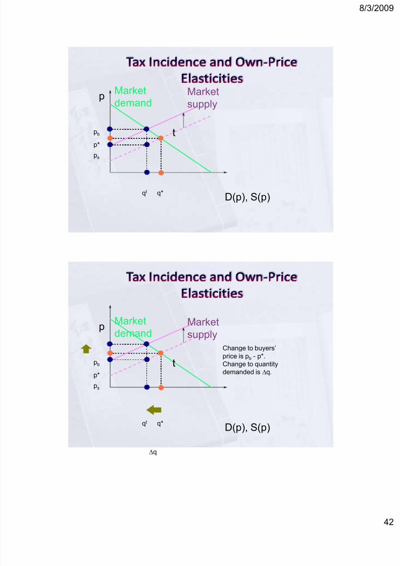
ps
Change to buyers’
price is pb - p*.Change to quantitydemanded is Dq.
Dq

7/27/2019 Economics 102 Lecture 10 Market Equilibrium Rev
http://slidepdf.com/reader/full/economics-102-lecture-10-market-equilibrium-rev 43/62
8/3/200
4
Around p = p* the own-price elasticity of demand is approximately
Db
q
q
p p
p
D
*
*
*
Around p = p* the own-price elasticity of demand is approximately
D
bb
D
q
q
p p
p
p p
q p
q
D
D*
*
*
**
* .

7/27/2019 Economics 102 Lecture 10 Market Equilibrium Rev
http://slidepdf.com/reader/full/economics-102-lecture-10-market-equilibrium-rev 44/62
8/3/200
4
p
D(p), S(p)
Market
demandMarketsupply
p*
q*
$tpb
qt
ps
p
D(p), S(p)
Marketdemand
Marketsupply
p*
q*
tpb
qt
ps
Change to sellers’
price is ps - p*.Change to quantitydemanded is Dq.
Dq

7/27/2019 Economics 102 Lecture 10 Market Equilibrium Rev
http://slidepdf.com/reader/full/economics-102-lecture-10-market-equilibrium-rev 45/62

7/27/2019 Economics 102 Lecture 10 Market Equilibrium Rev
http://slidepdf.com/reader/full/economics-102-lecture-10-market-equilibrium-rev 46/62
8/3/200
4
p
D(p), S(p)
Market
demandMarketsupply
p*
q*
pbpb
qt
pb
ps
Tax paid bybuyers
Tax paid bysellers
p
D(p), S(p)
Marketdemand
Marketsupply
p*
q*
pbpb
qt
pb
ps
Tax paid bybuyers
Tax paid by
sellers
Tax incidence =p p
p p
b
s
*
*.

7/27/2019 Economics 102 Lecture 10 Market Equilibrium Rev
http://slidepdf.com/reader/full/economics-102-lecture-10-market-equilibrium-rev 47/62
8/3/200
4
Tax incidence =p p
p p
b
s
*
*.
p pq p
qb
D
**
*.
p pq p
qs
S
**
*.
So p p
p p
b
s
S
D
*
* .
p p
p p
b
s
S
D
*
*.
Tax incidence is =
The fraction of a t quantity tax paid by buyersrises as supply becomes more own-price elasticor as demand becomes less own-price elastic.

7/27/2019 Economics 102 Lecture 10 Market Equilibrium Rev
http://slidepdf.com/reader/full/economics-102-lecture-10-market-equilibrium-rev 48/62
8/3/200
4
Special cases of taxation: Perfectly elasticsupply the price is entirely determined by the supply curve and
the quantity sold is determined by demand
Imposing a tax is just like shifting the supply curve bythe amount of the tax.
The supply price is the same as before and demandersend up paying the entire tax.
Since the industry is willing to supply any amount at certain price p* and zero amounts at another price, then
if any good will be sold at all, then the price that suppliers receive must be p*.
This determines the equilibrium supply price and thedemand price is p* +t.
p
D(p), S(p)
Marketdemand
Marketsupply
p*
q*
t
qt
As market supplybecomes more own-price elastic, taxincidence shifts more
to the buyers.
p*+ t

7/27/2019 Economics 102 Lecture 10 Market Equilibrium Rev
http://slidepdf.com/reader/full/economics-102-lecture-10-market-equilibrium-rev 49/62
8/3/200
4
Special case of taxation: Perfectly inelastic
supply
The quantity of the good is fixed and the equilibrium
price of a good is determined entirely by demand.
The supply curve just slides along itself and we still
have the same amount of the good supplied, with or
without the tax.
Demanders determine the equilibrium price of the good
and they are willing to pay p* for the supply of the goodthat is available, tax or no tax. Thus the demand price is
p* and the suppliers end up receiving p*-t.
The entire amount of the tax is paid by the suppliers.
p
D(p), S(p)
Marketdemand
Marketsupply
p*
t
qt = q*
As market supplybecomes less own-price elastic, taxincidence shifts more
to the sellers.p*- t

7/27/2019 Economics 102 Lecture 10 Market Equilibrium Rev
http://slidepdf.com/reader/full/economics-102-lecture-10-market-equilibrium-rev 50/62
8/3/200
5
Ordinary cases
Amount of the tax that gets passed along will
depend on the steepness of the demand curve
relative to the supply curve
If the supply curve is nearly horizontal, nearly all
of the tax gets passed along to the consumers.
If the supply curve is nearly vertical, almost none
of the tax gets passed along to the consumers.
p
D(p), S(p)
Marketdemand
Marketsupply
p*
q*
tpb
qt
ps
As market demandbecomes less own-price elastic, taxincidence shifts more
to the buyers.

7/27/2019 Economics 102 Lecture 10 Market Equilibrium Rev
http://slidepdf.com/reader/full/economics-102-lecture-10-market-equilibrium-rev 51/62
8/3/200
5
p
D(p), S(p)
Market
demandMarketsupply
p*
q*
tpb
qt
ps
As market demandbecomes less own-price elastic, taxincidence shifts moreto the buyers.
p
D(p), S(p)
Marketdemand
Marketsupply
p*
q*
tpb
qt
ps
As market demandbecomes less own-price elastic, taxincidence shifts more
to the buyers.
7/27/2019 Economics 102 Lecture 10 Market Equilibrium Rev
http://slidepdf.com/reader/full/economics-102-lecture-10-market-equilibrium-rev 52/62
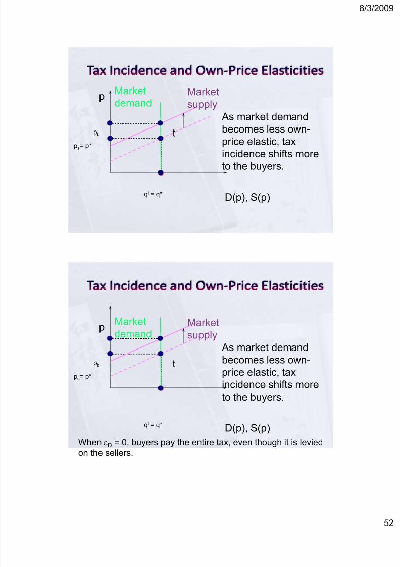
8/3/200
5
p
D(p), S(p)
Market
demandMarketsupply
ps= p*
tpb
qt = q*
As market demandbecomes less own-price elastic, taxincidence shifts moreto the buyers.
p
D(p), S(p)
Marketdemand
Marketsupply
ps= p*
tpb
qt = q*
As market demandbecomes less own-price elastic, taxincidence shifts more
to the buyers.
When D = 0, buyers pay the entire tax, even though it is leviedon the sellers.

7/27/2019 Economics 102 Lecture 10 Market Equilibrium Rev
http://slidepdf.com/reader/full/economics-102-lecture-10-market-equilibrium-rev 53/62
8/3/200
5
Welfare effects of a tax From the society’s viewpoint, the real cost of a tax is lost
output.
Social cost of a tax can be explored utilizing consumers’ andproducers’ surplus.
the loss in consumers’ surplus is the area A+B
the loss in producers’ surplus is given by the area C+D.
Is there any party that gains what the producers and theconsumers lose? This party is the government and it gainspart of the loss in consumer and producer surplus in the
form of tax revenue. Suppose that tax revenues will be utilized to provide services
to consumers and producers, then the net benefit to thegovernment is the area A+C.
p
D(p), S(p)
Marketdemand
Marketsupply
p*
q*
No tax

7/27/2019 Economics 102 Lecture 10 Market Equilibrium Rev
http://slidepdf.com/reader/full/economics-102-lecture-10-market-equilibrium-rev 54/62
8/3/200
5
p
D(p), S(p)
Market
demandMarketsupply
p*
q*
No taxCS
p
D(p), S(p)
Marketdemand
Marketsupply
p*
q*
No tax
PS

7/27/2019 Economics 102 Lecture 10 Market Equilibrium Rev
http://slidepdf.com/reader/full/economics-102-lecture-10-market-equilibrium-rev 55/62
8/3/200
5
p
D(p), S(p)
Market
demandMarketsupply
p*
q*
No taxCS
PS
p
D(p), S(p)
Marketdemand
Marketsupply
p*
q*
No taxCS
PS

7/27/2019 Economics 102 Lecture 10 Market Equilibrium Rev
http://slidepdf.com/reader/full/economics-102-lecture-10-market-equilibrium-rev 56/62
8/3/200
5
p
D(p), S(p)
Market
demandMarketsupply
p*
q*
tpb
qt
ps
CS
PS
The tax reducesboth CS and PS
A
C
B
D
p
D(p), S(p)
Marketdemand
Marketsupply
p*
q*
tpb
qt
ps
CS
PS
The tax reducesboth CS and PS,transfers surplusto governmentTax

7/27/2019 Economics 102 Lecture 10 Market Equilibrium Rev
http://slidepdf.com/reader/full/economics-102-lecture-10-market-equilibrium-rev 57/62
8/3/200
5
p
D(p), S(p)
Market
demandMarketsupply
p*
q*
tpb
qt
ps
CS
PS
The tax reducesboth CS and PS,transfers surplusto governmentTax
p
D(p), S(p)
Marketdemand
Marketsupply
p*
q*
tpb
qt
ps
CS
PS
The tax reducesboth CS and PS,transfers surplusto governmentTax

7/27/2019 Economics 102 Lecture 10 Market Equilibrium Rev
http://slidepdf.com/reader/full/economics-102-lecture-10-market-equilibrium-rev 58/62
8/3/200
5
p
D(p), S(p)
Market
demandMarketsupply
p*
q*
tpb
qt
ps
CS
PS
The tax reducesboth CS and PS,transfers surplusto government,and lowers total
surplus.
Tax
p
D(p), S(p)
Marketdemand
Marketsupply
p*
q*
tpb
qt
ps
CS
PS
Tax
Deadweight loss = B + D

7/27/2019 Economics 102 Lecture 10 Market Equilibrium Rev
http://slidepdf.com/reader/full/economics-102-lecture-10-market-equilibrium-rev 59/62
8/3/200
5
p
D(p), S(p)
Market
demandMarketsupply
p*
q*
tpb
qt
psDeadweight loss
p
D(p), S(p)
Marketdemand
Marketsupply
p*
q*
tpb
qt
ps
Deadweight loss fallsas market demandbecomes less own-price elastic.

7/27/2019 Economics 102 Lecture 10 Market Equilibrium Rev
http://slidepdf.com/reader/full/economics-102-lecture-10-market-equilibrium-rev 60/62
8/3/200
6
p
D(p), S(p)
Market
demandMarketsupply
p*
q*
tpb
qt
ps
Deadweight loss fallsas market demandbecomes less own-price elastic.
p
D(p), S(p)
Marketdemand
Marketsupply
ps= p*
tpb
qt = q*
Deadweight loss fallsas market demandbecomes less own-price elastic.
When D = 0, the tax causes no deadweight loss.

7/27/2019 Economics 102 Lecture 10 Market Equilibrium Rev
http://slidepdf.com/reader/full/economics-102-lecture-10-market-equilibrium-rev 61/62
8/3/200
6
The total net cost of the tax is the algebraic sum of the net benefits and the net costs: -(A+B) –(C+D) +(A+C)= –(B+D).
This area is know as the deadweight loss of the taxor the excess burden of the tax.
Source of excess burden – It is the lost value toconsumers and producers due to the reduction insales of the good.
We could also derive the deadweight loss directly byjust measuring the social value of the lost output. Demand price measures how much a consumer was willing
to pay for the good and the supply price measures the priceat which somebody was willing to supply. The difference isthe lost value on that unit of the good.
Is a competitive market Pareto efficient?
Competitive market determines how much is
produced based on how much people are willing
to pay to purchase the good as compared to how
much people must be paid to produce the good.
If a good were produced and exchanged between
these two people at any price between the
demand price and the supply price, they would
both be made better off.

7/27/2019 Economics 102 Lecture 10 Market Equilibrium Rev
http://slidepdf.com/reader/full/economics-102-lecture-10-market-equilibrium-rev 62/62
8/3/200
Competitive market produces a Pareto efficient amount of output.
In a competitive market, everyone pays the same priceof the good and this price is the marginal rate of substitution between the good and all other goods.
If the MRS is not the same, then there must be at least two people who value a unit of the good differently.Thus any allocation with different marginal rates of substitution cannot be Pareto efficient.