Economics 371Economics 371Economics 371Economics 371Labor EconomicsLabor Economics

unemployment

labor unions welfare programs

education

discrimination

minimum wages

income taxes

diminishing returns

monopsony

occupational licensing

job search

Course Essentials

• Course Web Page– www.marietta.edu/~delemeeg/econ37

1

• Grades– Exams (60%)– Homework (20%)– Policy/Market Brief (20%)

• Course Web Page– www.marietta.edu/~delemeeg/econ37

1

• Grades– Exams (60%)– Homework (20%)– Policy/Market Brief (20%)

Economic Way of Thinking Rationality Marginal analysis Scarcity Positive vs. normative analysis

Rationality Marginal analysis Scarcity Positive vs. normative analysis

Economic Models

Objectives Constraints Behavior

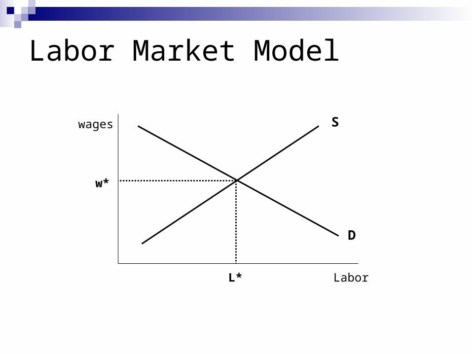
Labor Market Model

S

D

Labor

wages

w*

L*

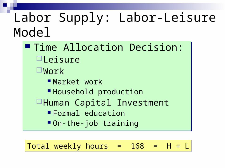
Labor Supply: Labor-Leisure Model

Time Allocation Decision:LeisureWork

Market work Household production

Human Capital Investment Formal education On-the-job training

Time Allocation Decision:LeisureWork

Market work Household production

Human Capital Investment Formal education On-the-job training

Total weekly hours = 168 = H + LTotal weekly hours = 168 = H + L

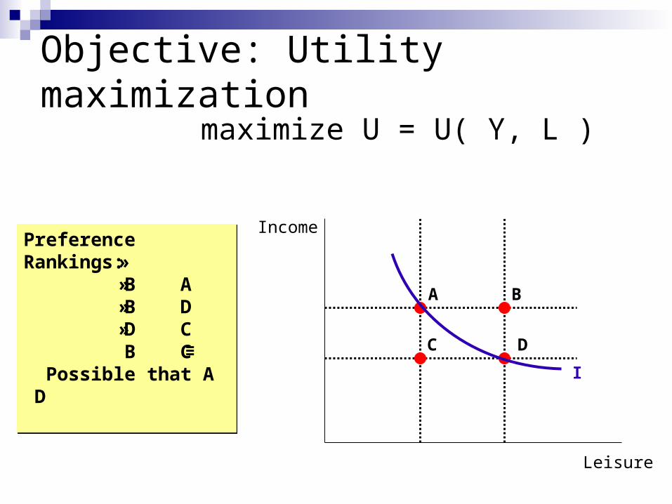
Objective: Utility maximization

maximize U = U( Y, L )

Leisure

Income

A B

C D

Preference Rankings: B A B D D C B C Possible that A D

Preference Rankings: B A B D D C B C Possible that A D

I

»≡

»»»

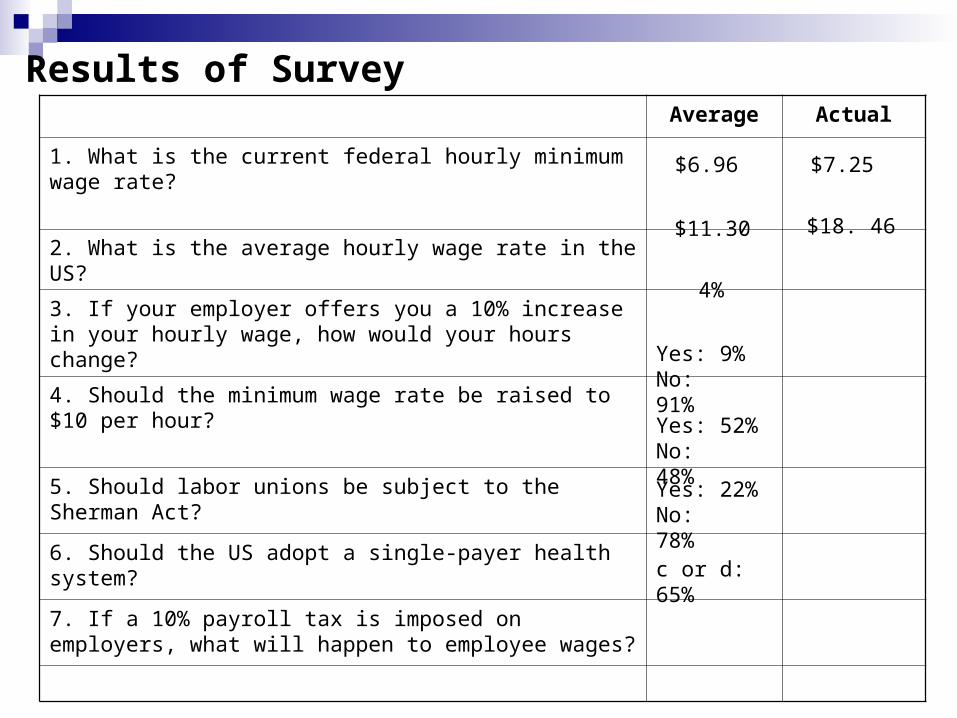
Average Actual

1. What is the current federal hourly minimum wage rate?

2. What is the average hourly wage rate in the US?

3. If your employer offers you a 10% increase in your hourly wage, how would your hours change?

4. Should the minimum wage rate be raised to $10 per hour?

5. Should labor unions be subject to the Sherman Act?

6. Should the US adopt a single-payer health system?

7. If a 10% payroll tax is imposed on employers, what will happen to employee wages?

$7.25$6.96

$11.30 $18. 46

Yes: 9%No: 91%

Yes: 52%No: 48%

Yes: 22%No: 78%

c or d: 65%

4%

Results of Survey

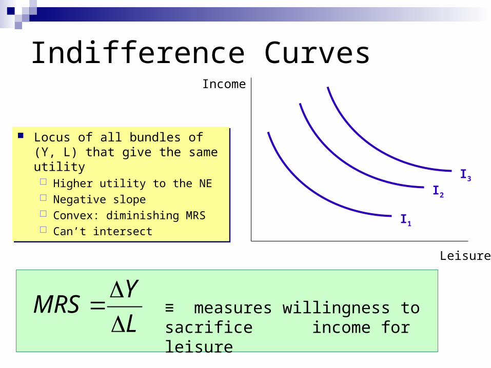
Indifference Curves

Locus of all bundles of (Y, L) that give the same utility Higher utility to the NE Negative slope Convex: diminishing MRS Can’t intersect

Locus of all bundles of (Y, L) that give the same utility Higher utility to the NE Negative slope Convex: diminishing MRS Can’t intersect

Leisure

Income

I2

I1

I3

L

YMRS

≡ measures willingness to sacrifice income for leisure

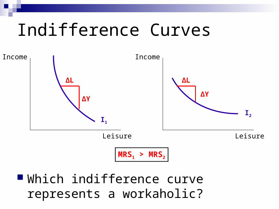
Indifference Curves

Which indifference curve represents a workaholic?

Leisure

Income

I1

Leisure

Income

I2

ΔL ΔL

ΔYΔY

MRS1 > MRS2

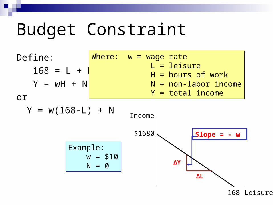
Budget Constraint

Define: 168 = L + H Y = wH + Nor

Y = w(168-L) + N

Where: w = wage rate L = leisure H = hours of work N = non-labor income Y = total income

Where: w = wage rate L = leisure H = hours of work N = non-labor income Y = total income

Leisure

Income

Example: w = $10 N = 0

Example: w = $10 N = 0

168

$1680 Slope = - w

ΔL

ΔY

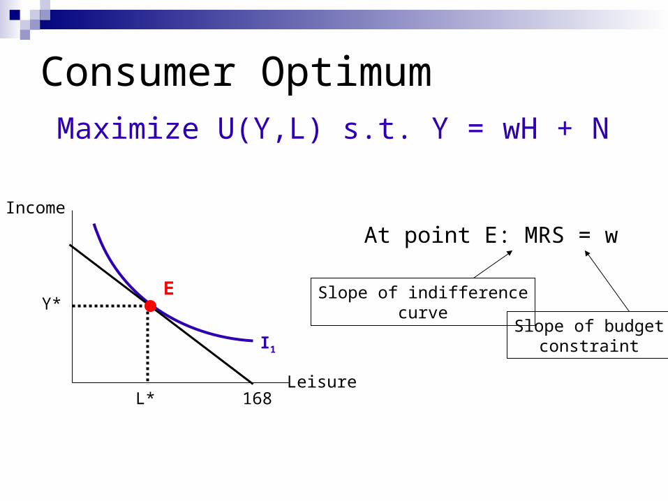
Consumer OptimumMaximize U(Y,L) s.t. Y = wH + N

Leisure

Income

I1

L*

Y*

168

E

At point E: MRS = w

Slope of indifferencecurve

Slope of budgetconstraint

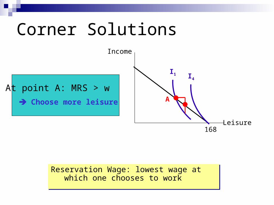
Corner Solutions

Reservation Wage: lowest wage at which one chooses to work

Reservation Wage: lowest wage at which one chooses to work

Leisure

Income

I1

168

I4

A

At point A: MRS > w

Choose more leisure

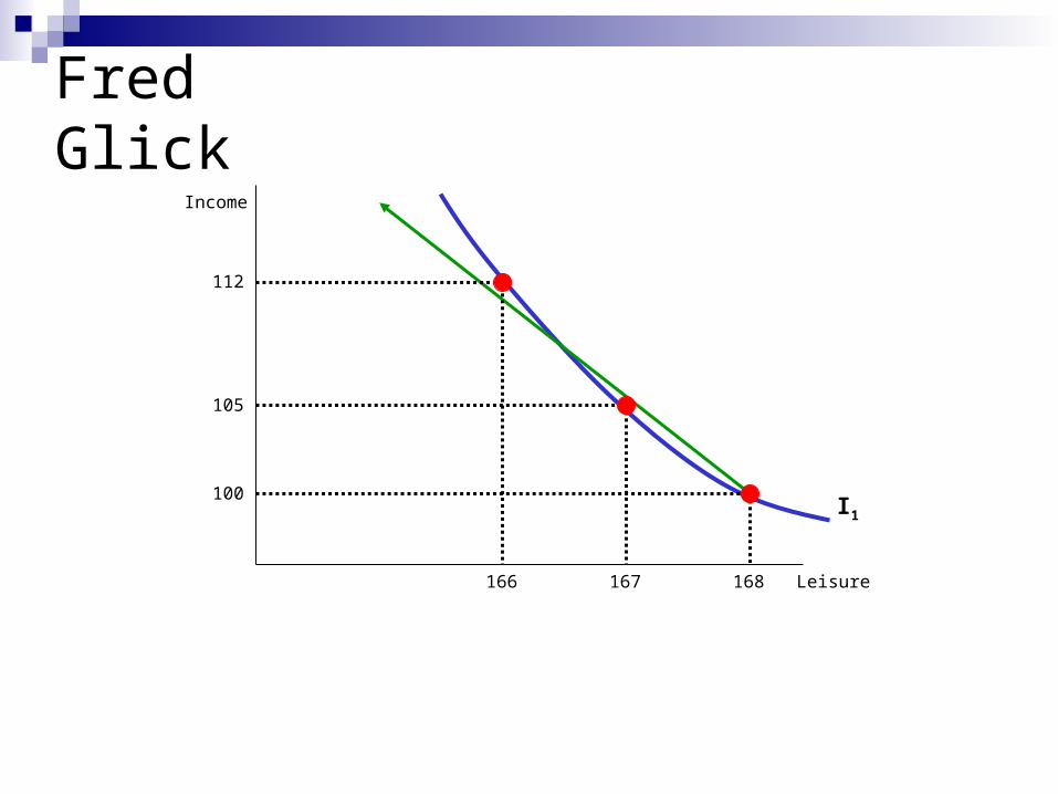
Fred Glick

Leisure

Income

168

100I1

112

105

167166

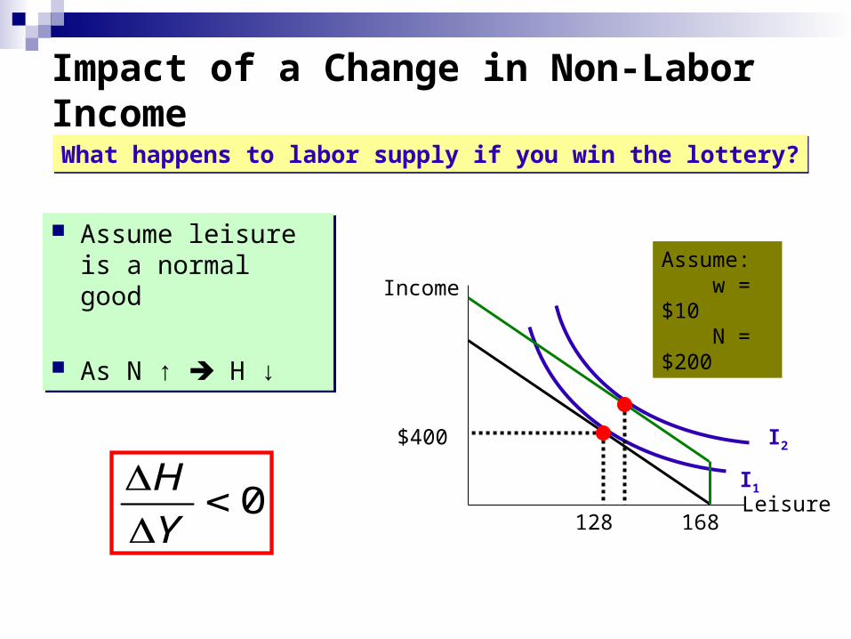
Impact of a Change in Non-Labor Income

Assume leisure is a normal good

As N ↑ H ↓

Assume leisure is a normal good

As N ↑ H ↓

Leisure

Income

I1

128

$400

168

Assume: w = $10 N = $200

I2

What happens to labor supply if you win the lottery?What happens to labor supply if you win the lottery?

0Y

H

Labor Supply and the Lottery

Source: Kimball, Miles S. and Matthew D. Shapiro. “Labor Supply: Are the Income and Substitution Effects Both Large or Both Small?” Working Paper, May 16, 2003. Accessed online at www-personal.umich.edu/~mkimball/pdf/labor-16may2003.pdf.

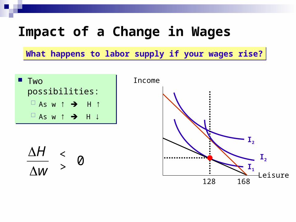
Impact of a Change in Wages

Two possibilities: As w ↑ H ↑ As w ↑ H ↓

Two possibilities: As w ↑ H ↑ As w ↑ H ↓

Leisure

Income

128 168

What happens to labor supply if your wages rise?What happens to labor supply if your wages rise?

w

H

<

> 0 I1

I2

I2

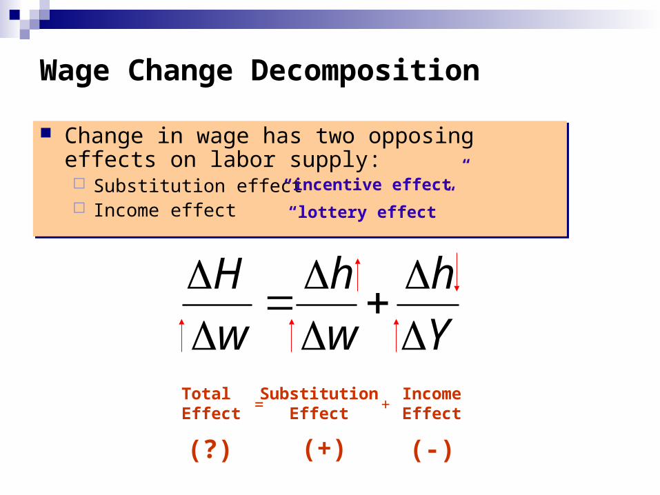
Wage Change Decomposition

Change in wage has two opposing effects on labor supply: Substitution effect Income effect

Change in wage has two opposing effects on labor supply: Substitution effect Income effect

“incentive effect”

“lottery effect”

Y

h

w

h

w

H

TotalEffect

SubstitutionEffect

IncomeEffect

(+) (-)(?)

= +

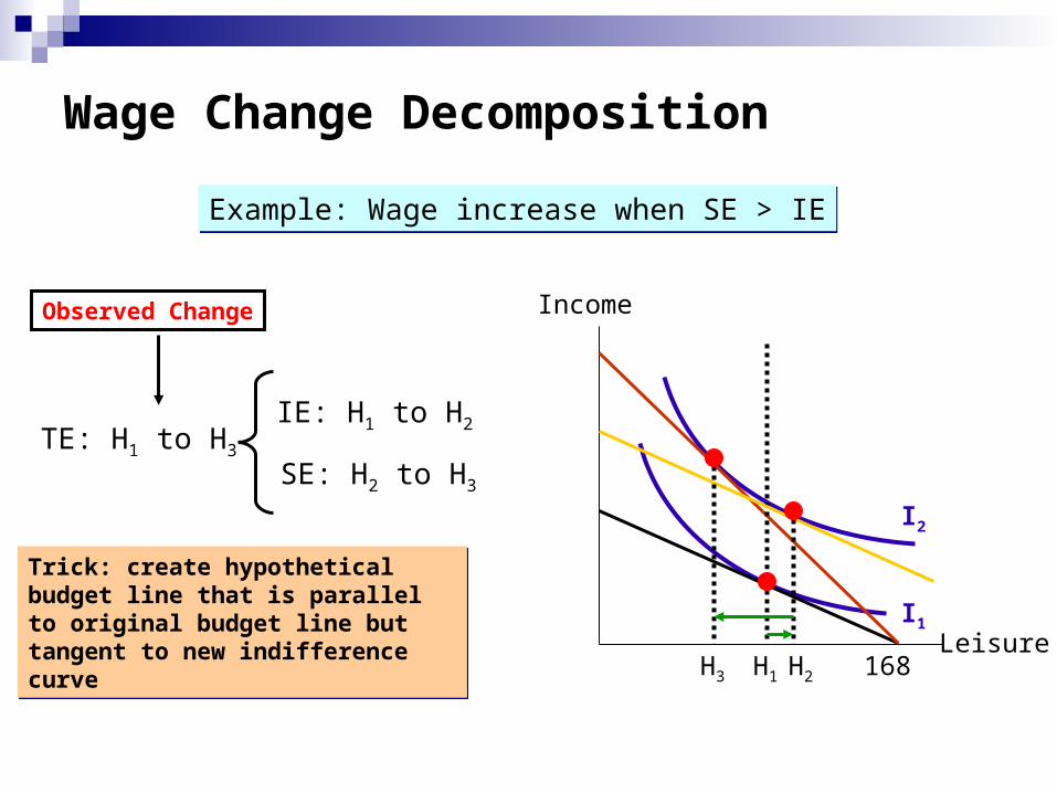
Wage Change Decomposition

Leisure

Income

H1 168

I1

I2

H2H3

TE: H1 to H3

IE: H1 to H2

SE: H2 to H3

Example: Wage increase when SE > IEExample: Wage increase when SE > IE

Observed Change

Trick: create hypothetical budget line that is parallel to original budget line but tangent to new indifference curve

Trick: create hypothetical budget line that is parallel to original budget line but tangent to new indifference curve

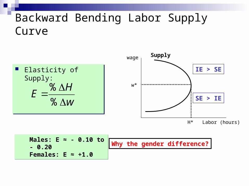
Backward Bending Labor Supply Curve

Elasticity of Supply: Elasticity of Supply:

Labor (hours)

wage

w*

H*

Supply

IE > SE

SE > IEw

HE

%

%

Why the gender difference?Males: E ≈ - 0.10 to - 0.20Females: E ≈ +1.0Males: E ≈ - 0.10 to - 0.20Females: E ≈ +1.0

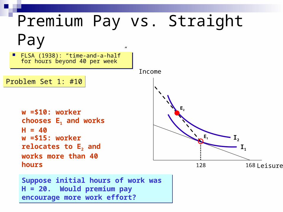
Premium Pay vs. Straight Pay FLSA (1938): “time-and-a-half”

for hours beyond 40 per week FLSA (1938): “time-and-a-half”

for hours beyond 40 per week

Leisure

Income

168128

I1

E1 I2

w =$10: worker chooses E1 and works H = 40

w =$15: worker relocates to E2 and works more than 40 hours

Suppose initial hours of work was H = 20. Would premium pay encourage more work effort?

Suppose initial hours of work was H = 20. Would premium pay encourage more work effort?

Problem Set 1: #10Problem Set 1: #10

E2

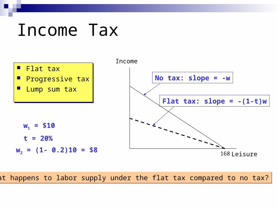
Income Tax

Flat tax Progressive tax Lump sum tax

Flat tax Progressive tax Lump sum tax

Leisure

Income

168

No tax: slope = -w

Flat tax: slope = -(1-t)w

What happens to labor supply under the flat tax compared to no tax?What happens to labor supply under the flat tax compared to no tax?

w1 = $10

t = 20%

w2 = (1- 0.2)10 = $8

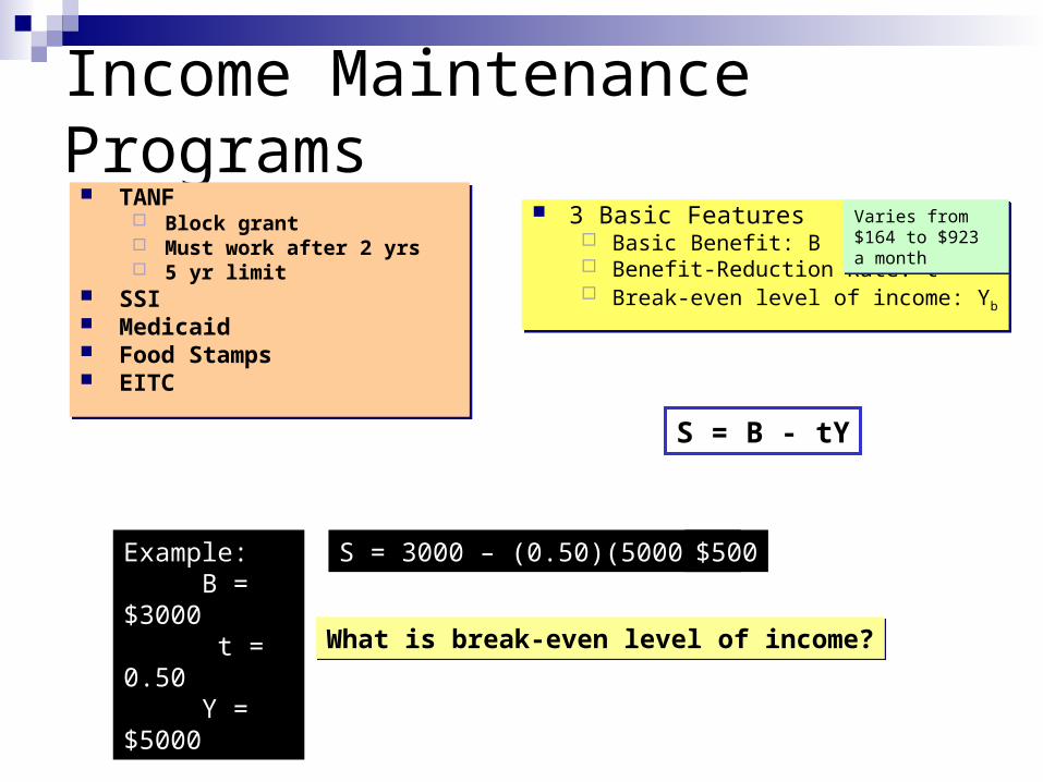
Income Maintenance Programs

TANF Block grant Must work after 2 yrs 5 yr limit

SSI Medicaid Food Stamps EITC

TANF Block grant Must work after 2 yrs 5 yr limit

SSI Medicaid Food Stamps EITC

3 Basic Features Basic Benefit: B Benefit-Reduction Rate: t Break-even level of income: Yb

3 Basic Features Basic Benefit: B Benefit-Reduction Rate: t Break-even level of income: Yb

S = B - tY

Example: B = $3000 t = 0.50 Y = $5000

S = 3000 – (0.50)(5000) = $500

What is break-even level of income?What is break-even level of income?

Varies from $164 to $923 a monthVaries from $164 to $923 a month

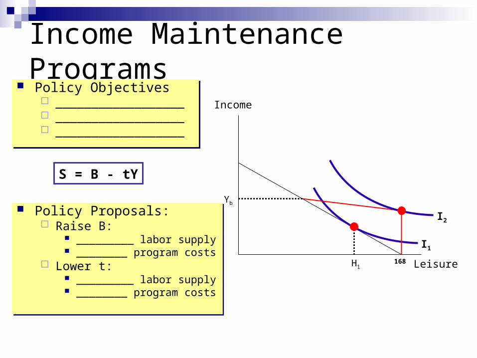
Income Maintenance Programs

Policy Proposals: Raise B:

_________ labor supply ________ program costs

Lower t: _________ labor supply ________ program costs

Policy Proposals: Raise B:

_________ labor supply ________ program costs

Lower t: _________ labor supply ________ program costs

Policy Objectives __________________ __________________ __________________

Policy Objectives __________________ __________________ __________________

Leisure

Income

168

Yb

I1

I2

S = B - tY

H1

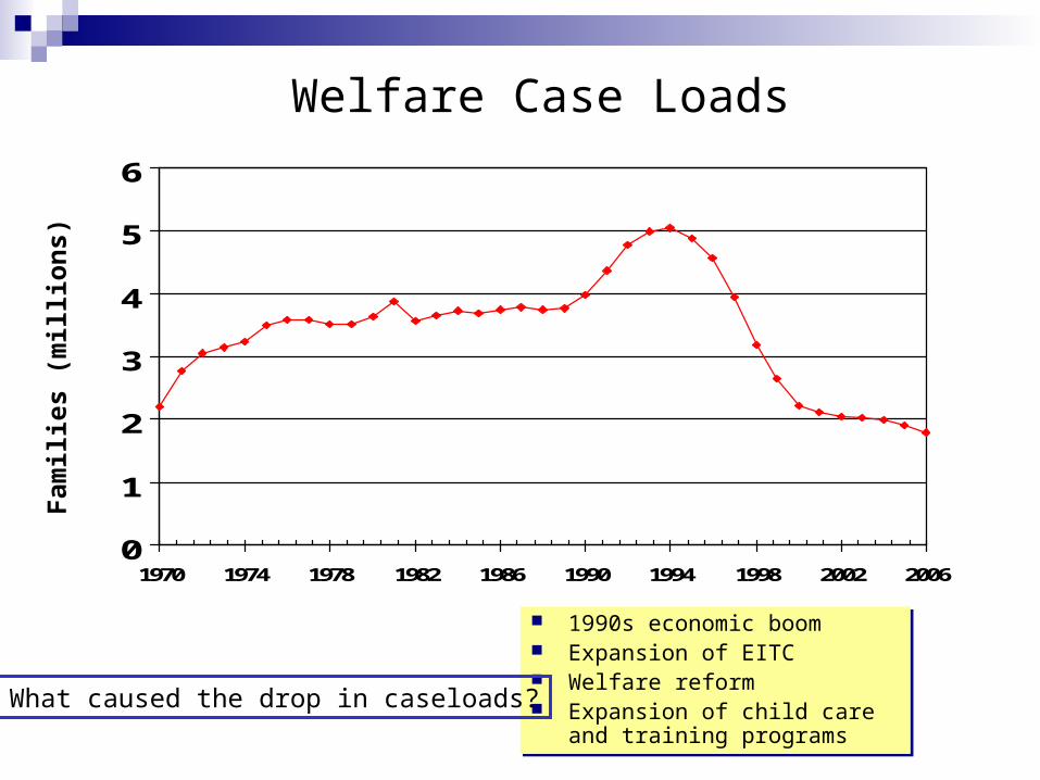
1990s economic boom Expansion of EITC Welfare reform Expansion of child care and

training programs

1990s economic boom Expansion of EITC Welfare reform Expansion of child care and

training programs

Fam

ilie

s (m

illi

on

s)

What caused the drop in caseloads?

0

1

2

3

4

5

6

1970 1974 1978 1982 1986 1990 1994 1998 2002 2006

Welfare Case Loads

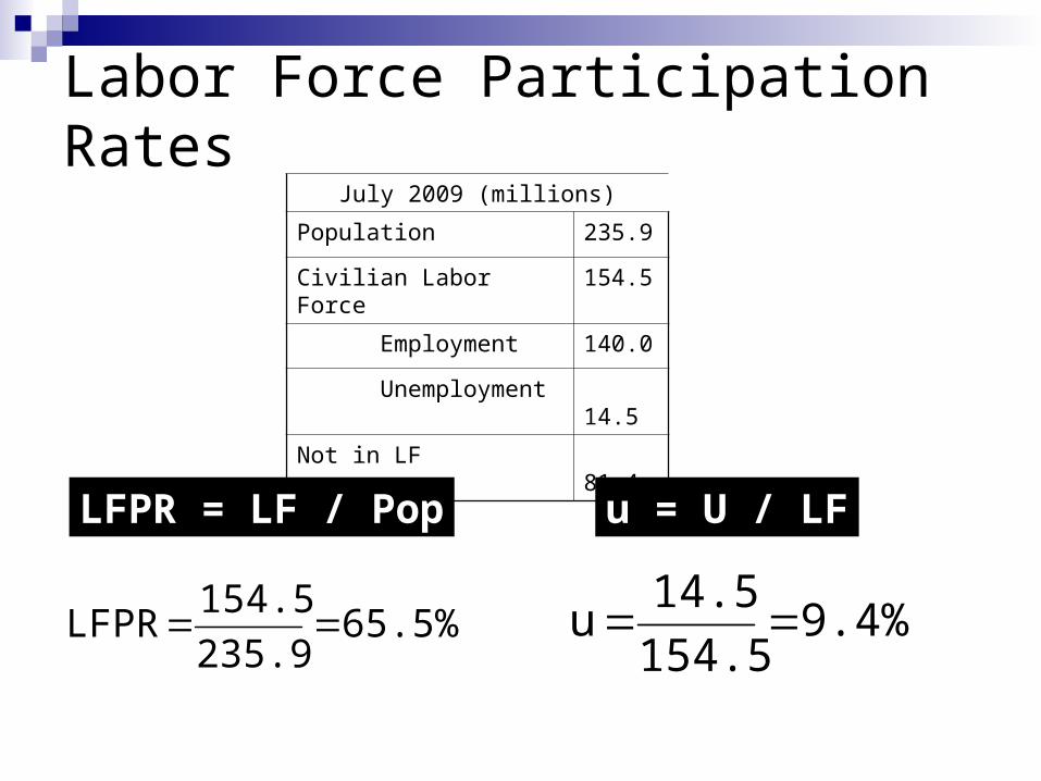
Labor Force Participation RatesJuly 2009 (millions)

Population 235.9

Civilian Labor Force 154.5

Employment 140.0

Unemployment 14.5

Not in LF 81.4

65.5%235.9154.5

LFPR

LFPR = LF / Pop u = U / LF

9.4%154.514.5

u

Per

cen

t

0

10

20

30

40

50

60

70

80

90

100

1950 1955 1960 1965 1970 1975 1980 1985 1990 1995 2000 2005

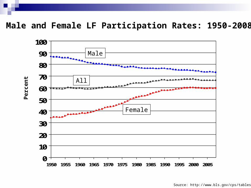
Male and Female LF Participation Rates: 1950-2008

Source: http://www.bls.gov/cps/tables.htm

Male

Female

All

Per

cen

t

0

10

20

30

40

50

60

70

80

90

100

1950 1955 1960 1965 1970 1975 1980 1985 1990 1995 2000 2005

20-24 25-54 55-64 65 and over

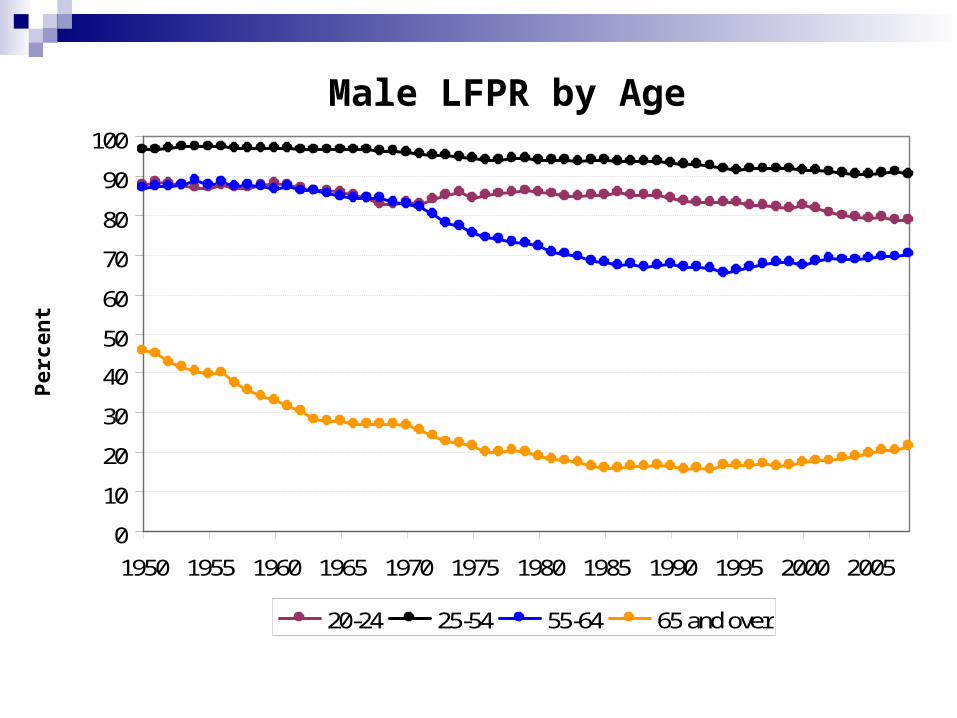
Male LFPR by Age

Per

cen

t

0

10

20

30

40

50

60

70

80

90

100

1950 1955 1960 1965 1970 1975 1980 1985 1990 1995 2000 2005

20-24 25-54 55-64 65 and over

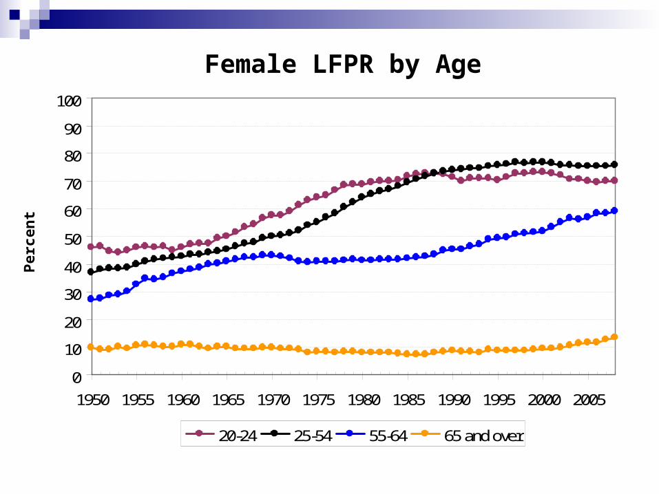
Female LFPR by Age

Per

cen

t

66

68

70

72

74

76

78

80

82

1970 1975 1980 1985 1990 1995 2000 2005

White African-American

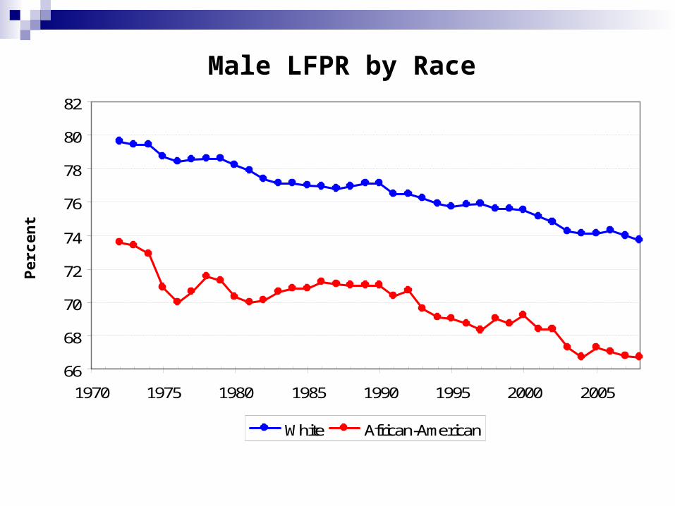
Male LFPR by Race

Per

cen

t

0

10

20

30

40

50

60

70

80

90

100

1970 1975 1980 1985 1990 1995 2000 2005

White African-American

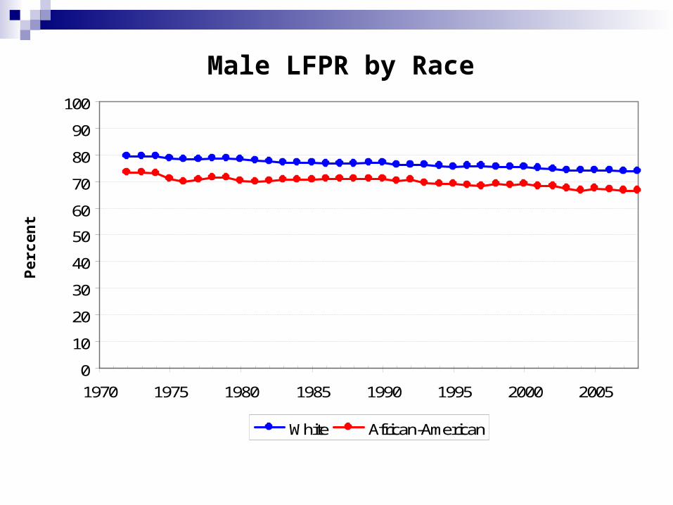
Male LFPR by Race

Per

cen

t

30

40

50

60

70

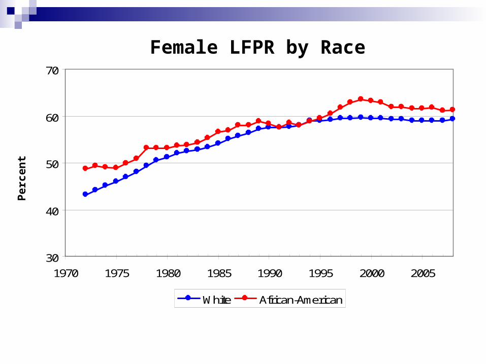
1970 1975 1980 1985 1990 1995 2000 2005

White African-American

Female LFPR by Race

Secular Trends in LFPR Falling male LFPR

_____________________________ _____________________________ _____________________________ _____________________________

Rising female LFPR _____________________________ _____________________________ _____________________________ _____________________________ _____________________________ _____________________________

Falling male LFPR _____________________________ _____________________________ _____________________________ _____________________________

Rising female LFPR _____________________________ _____________________________ _____________________________ _____________________________ _____________________________ _____________________________

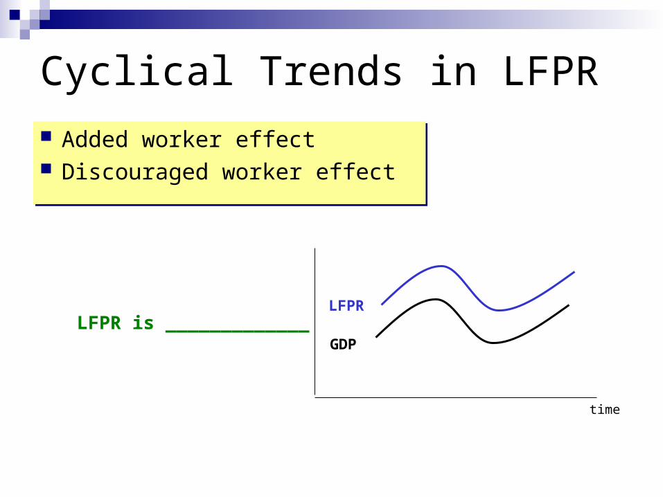
Added worker effect Discouraged worker effect

Added worker effect Discouraged worker effect

Cyclical Trends in LFPR

LFPR is _____________

time

GDP

LFPR

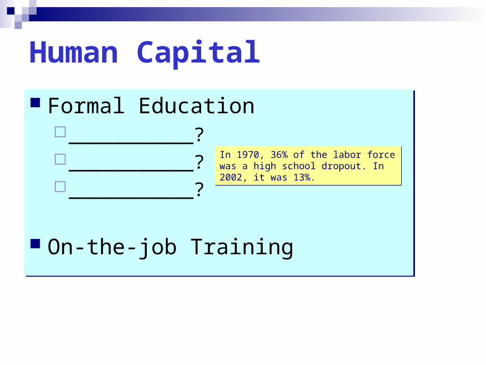
Human Capital

Formal Education___________?___________?___________?

On-the-job Training

Formal Education___________?___________?___________?

On-the-job Training

In 1970, 36% of the labor force was a high school dropout. In 2002, it was 13%.In 1970, 36% of the labor force was a high school dropout. In 2002, it was 13%.

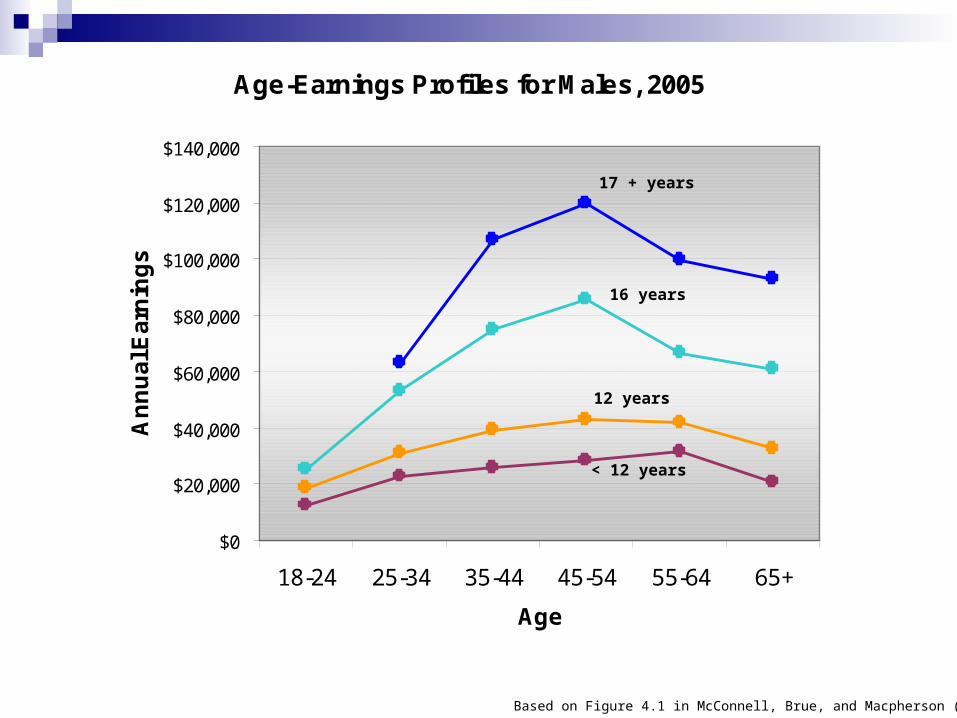
Age-Earnings Profiles for Males, 2005

$0

$20,000

$40,000

$60,000

$80,000

$100,000

$120,000

$140,000

18-24 25-34 35-44 45-54 55-64 65+

Age

An

nu

al E

arn

ing

s

Based on Figure 4.1 in McConnell, Brue, and Macpherson (2006)

17 + years

16 years

12 years

< 12 years

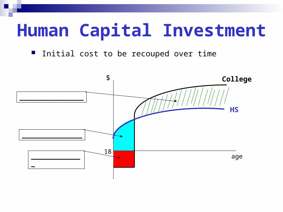
Initial cost to be recouped over time

Human Capital Investment

age

HS

College$

______________

________________

_________________

18

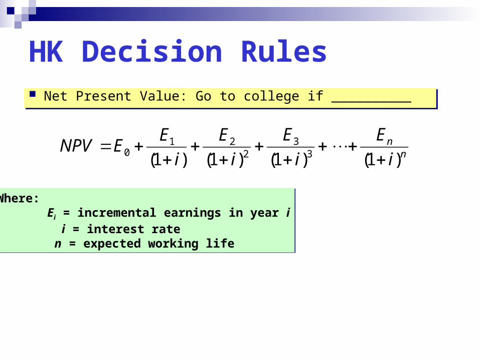
HK Decision Rules Net Present Value: Go to college if __________ Net Present Value: Go to college if __________

nn

i

E

i

E

i

E

i

EENPV

)1()1()1()1( 33

221

0

Where: Ei = incremental earnings in year i i = interest rate n = expected working life

Where: Ei = incremental earnings in year i i = interest rate n = expected working life

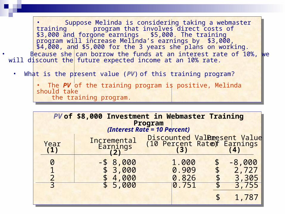
• Because she can borrow the funds at an interest rate of 10%, wewill discount the future expected income at an 10% rate.

• What is the present value (PV) of this training program?

• The PV of the training program is positive, Melinda should take the training program.

• Suppose Melinda is considering taking a webmaster training program that involves direct costs of $3,000 and forgone earnings $5,000. The training program will increase Melinda’s earnings by $3,000, $4,000, and $5,000 for the 3 years she plans on working.

Present Valueof Earnings

(4)

Discounted Value(10 Percent Rate)

(3)Incremental

Earnings(2)

Year(1)

PV of $8,000 Investment in Webmaster Training Program

(Interest Rate = 10 Percent)

0 -$ 8,000 1.000 $ -8,000123

$ 3,000 $ 4,000 $ 5,000

0.9090.8260.751

$ 2,727$ 3,305$ 3,755

$ 1,787

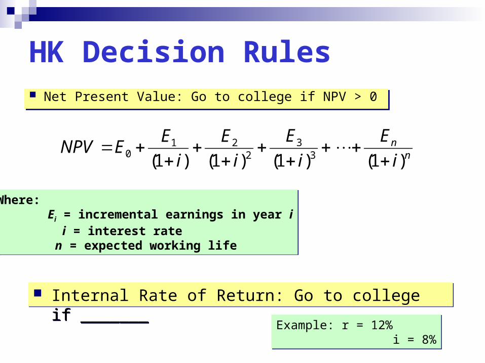
HK Decision Rules Net Present Value: Go to college if NPV > 0 Net Present Value: Go to college if NPV > 0

nn

i

E

i

E

i

E

i

EENPV

)1()1()1()1( 33

221

0

Where: Ei = incremental earnings in year i i = interest rate n = expected working life

Where: Ei = incremental earnings in year i i = interest rate n = expected working life

Internal Rate of Return: Go to college if _______ Internal Rate of Return: Go to college if _______

Example: r = 12% i = 8%Example: r = 12% i = 8%

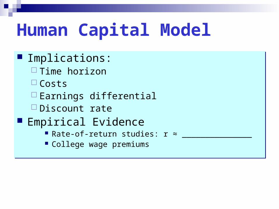
Human Capital Model Implications:

Time horizon Costs Earnings differential Discount rate

Empirical Evidence Rate-of-return studies: r ≈ _______________ College wage premiums

Implications: Time horizon Costs Earnings differential Discount rate

Empirical Evidence Rate-of-return studies: r ≈ _______________ College wage premiums

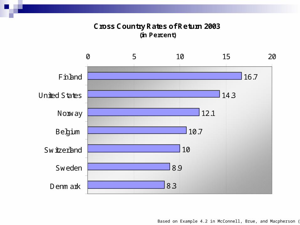
Cross Country Rates of Return 2003(in Percent)

16.7

14.3

12.1

10.7

10

8.9

8.3

0 5 10 15 20

Finland

United States

Norway

Belgium

Switzerland

Sweden

Denmark

Based on Example 4.2 in McConnell, Brue, and Macpherson (2006)

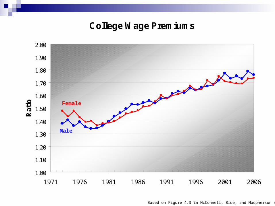
College Wage Premiums

1.00

1.10

1.20

1.30

1.40

1.50

1.60

1.70

1.80

1.90

2.00

1971 1976 1981 1986 1991 1996 2001 2006

Rat

io

Based on Figure 4.3 in McConnell, Brue, and Macpherson (2006)

Female

Male

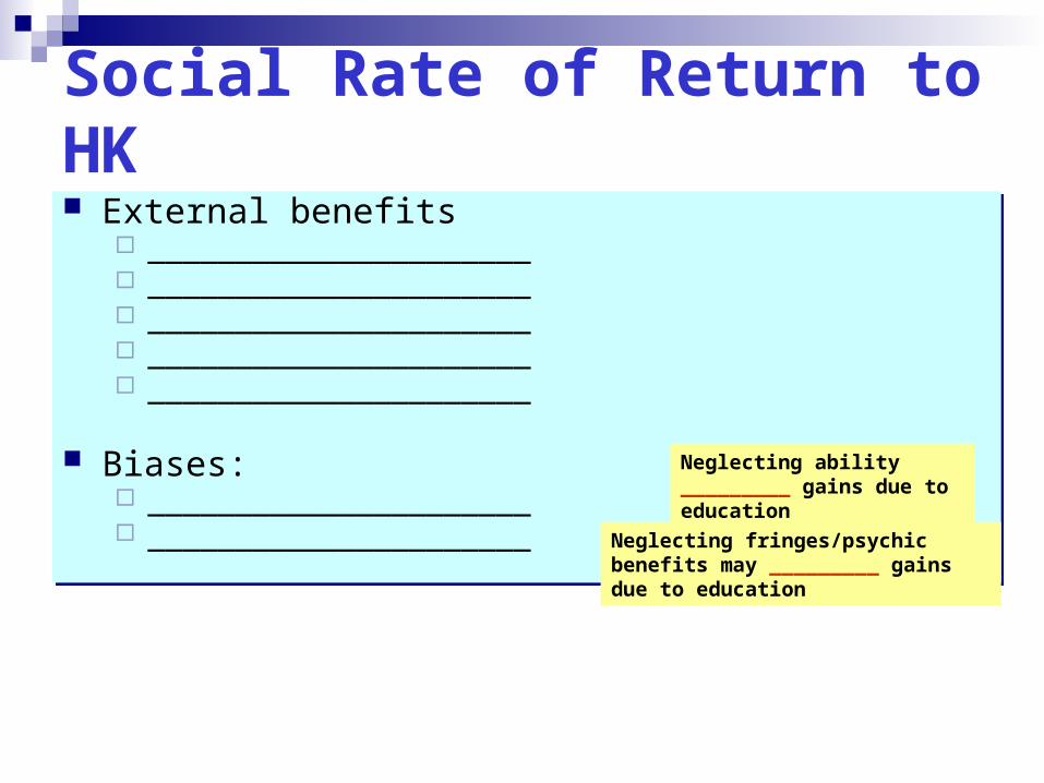
Social Rate of Return to HK External benefits

______________________ ______________________ ______________________ ______________________ ______________________

Biases: ______________________ ______________________

External benefits ______________________ ______________________ ______________________ ______________________ ______________________

Biases: ______________________ ______________________

Neglecting ability _________ gains due to education

Neglecting fringes/psychic benefits may _________ gains due to education

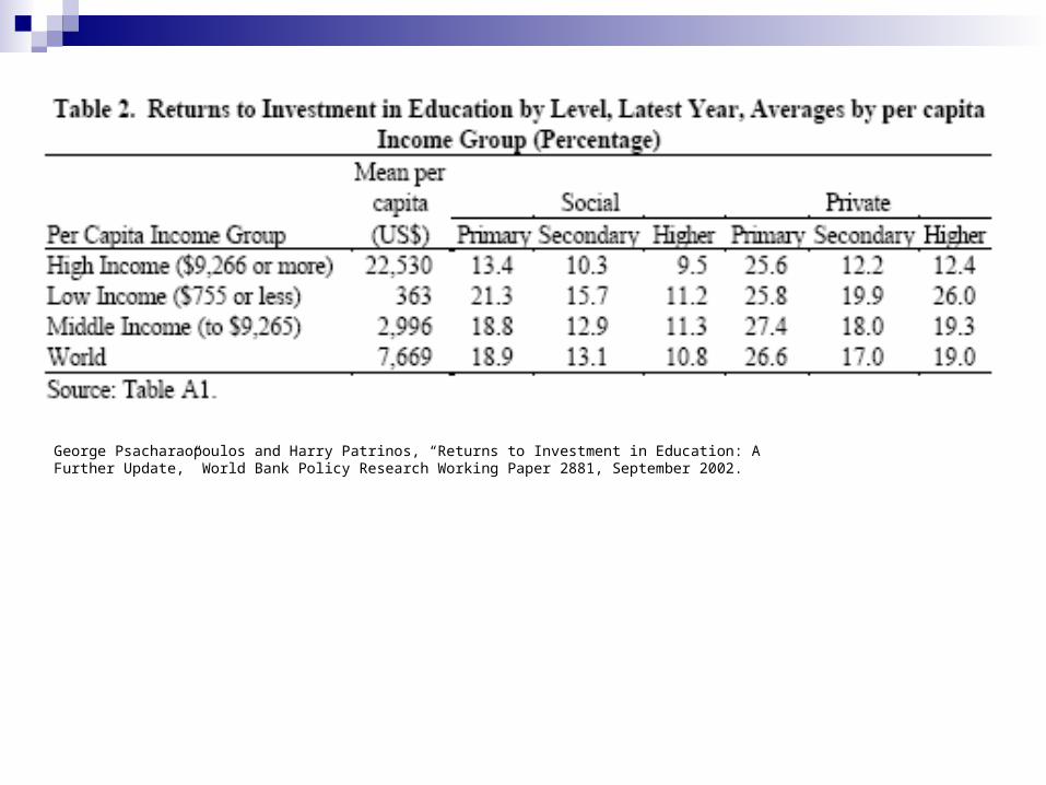
George Psacharaopoulos and Harry Patrinos, “Returns to Investment in Education: A Further Update,” World Bank Policy Research Working Paper 2881, September 2002.

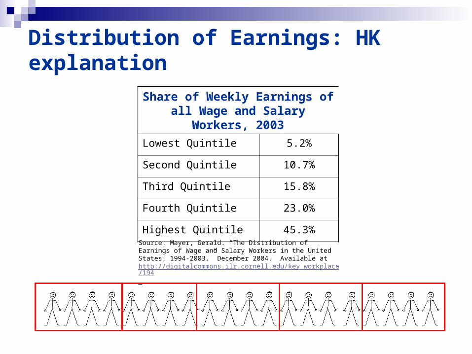
Share of Weekly Earnings of all Wage and Salary

Workers, 2003

Lowest Quintile 5.2%

Second Quintile 10.7%

Third Quintile 15.8%

Fourth Quintile 23.0%

Highest Quintile 45.3%

Source: Mayer, Gerald. “The Distribution of Earnings of Wage and Salary Workers in the United States, 1994-2003.” December 2004. Available at http://digitalcommons.ilr.cornell.edu/key_workplace/194

Distribution of Earnings: HK explanation

Distribution of Earnings: HK explanation

Differences in HK investment __________________ __________________ __________________

Capital market imperfections __________________ __________________

Differences in HK investment __________________ __________________ __________________

Capital market imperfections __________________ __________________

DA

DB

education

r(%)

r1

r2

e1 e2

Demand: diminishing returns to educationSupply: perfectly elasticDemand: diminishing returns to educationSupply: perfectly elastic

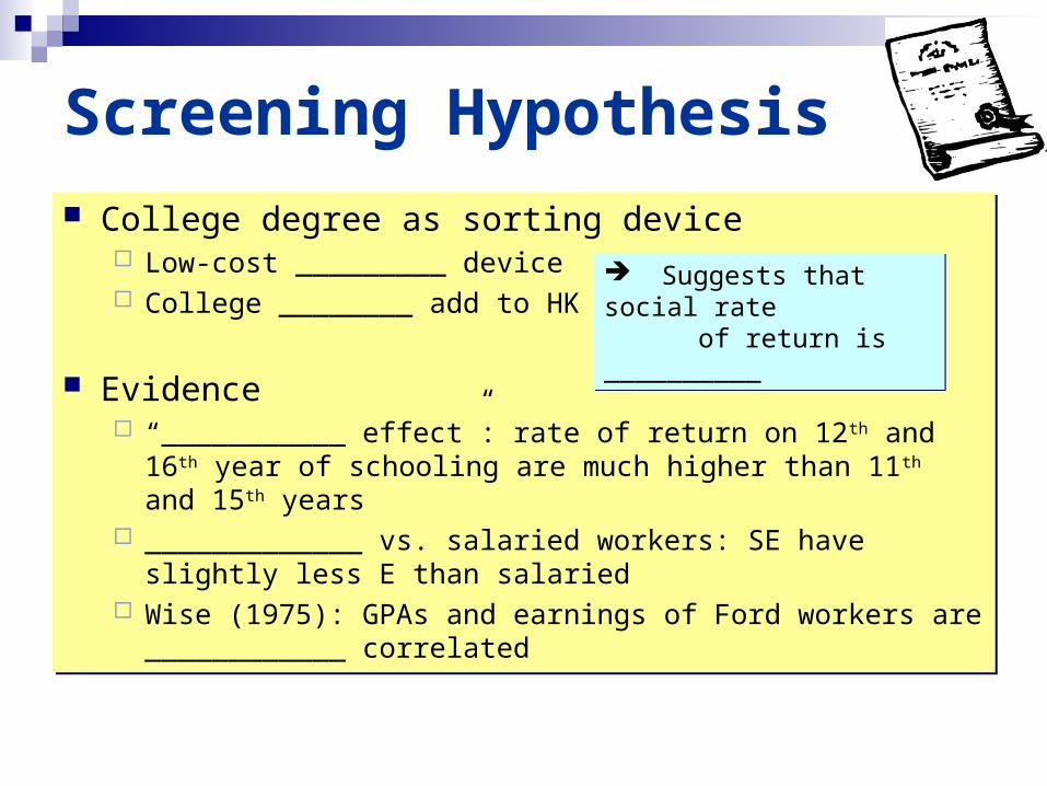
Screening Hypothesis College degree as sorting device

Low-cost _________ device College ________ add to HK

Evidence “___________ effect”: rate of return on 12th and 16th year

of schooling are much higher than 11th and 15th years _____________ vs. salaried workers: SE have slightly less E

than salaried Wise (1975): GPAs and earnings of Ford workers are

____________ correlated

College degree as sorting device Low-cost _________ device College ________ add to HK

Evidence “___________ effect”: rate of return on 12th and 16th year

of schooling are much higher than 11th and 15th years _____________ vs. salaried workers: SE have slightly less E

than salaried Wise (1975): GPAs and earnings of Ford workers are

____________ correlated

Suggests that social rate of return is __________

Suggests that social rate of return is __________

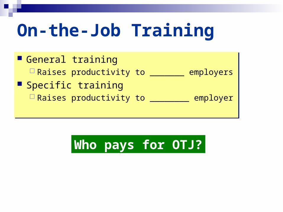
On-the-Job Training

General training Raises productivity to _______ employers

Specific training Raises productivity to ________ employer

General training Raises productivity to _______ employers

Specific training Raises productivity to ________ employer

Who pays for OTJ?

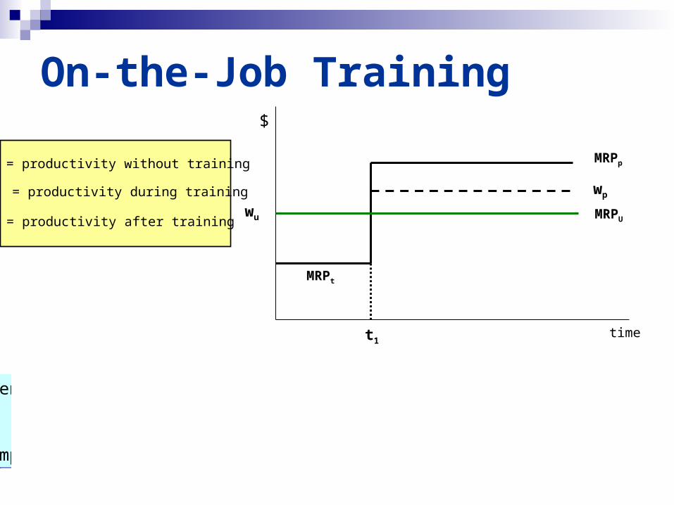
Specific Training: MRPu < wp < MRPp

wt = MRPu

Employer pays for training; employeeis exploited after training

Specific Training: MRPu < wp < MRPp

wt = MRPu

Employer pays for training; employeeis exploited after training

On-the-Job Training

MRPt

MRPp

time

wu

t1

MRPU

MRPt = productivity during training

MRPp = productivity after training

MRPu = productivity without training

General Training: wp = MRPp

wt = MRPt

Employee pays thru low training wage

General Training: wp = MRPp

wt = MRPt

Employee pays thru low training wage

wp

$

Source: http://www.advicenow.org.uk/go/feature/feature_357.html?pkgid=35

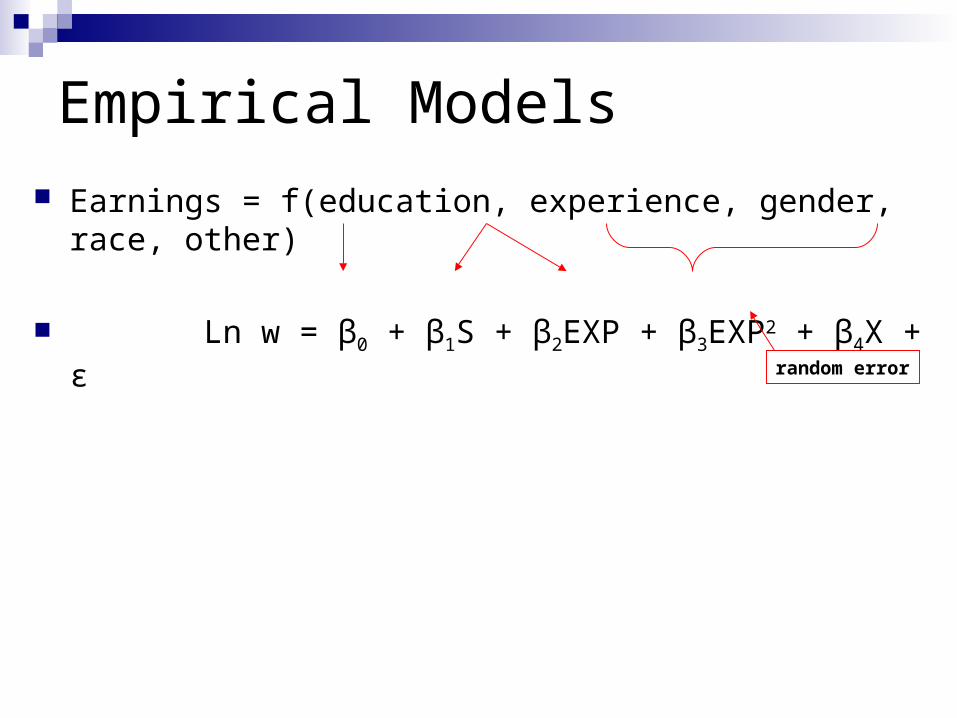
Empirical Models Earnings = f(education, experience, gender, race,

other)

Ln w = β0 + β1S + β2EXP + β3EXP2 + β4X + εrandom error