economics of taxation - coin.wne.uw.edu.plcoin.wne.uw.edu.pl/gkula/economics of taxation 3.pdf ·...
TRANSCRIPT
Economics of taxation
Lecture 3: Optimal taxation theories Salanie (2003)
dr Grzegorz Kula, [email protected]
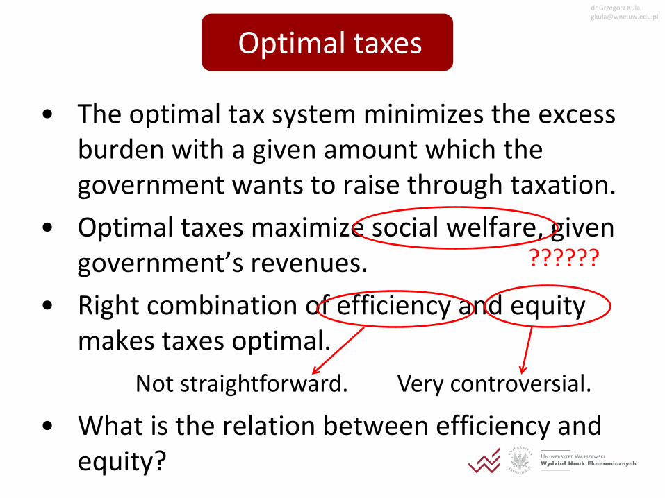
• The optimal tax system minimizes the excess burden with a given amount which the government wants to raise through taxation.
• Optimal taxes maximize social welfare, given government’s revenues.
• Right combination of efficiency and equity makes taxes optimal.
• What is the relation between efficiency and equity?
Optimal taxes
??????
Not straightforward. Very controversial.
dr Grzegorz Kula, [email protected]
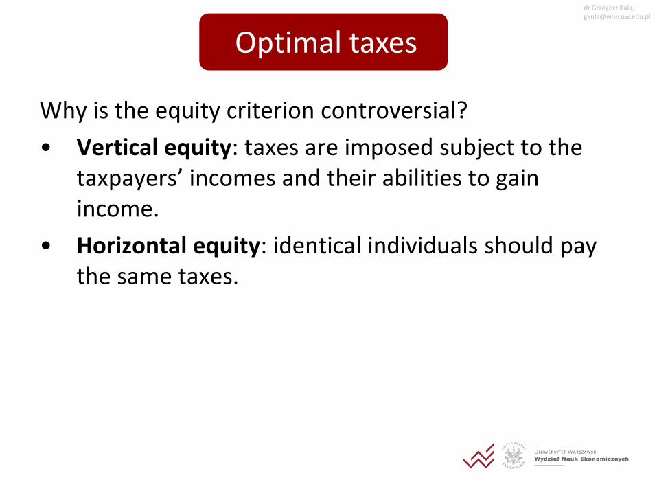
Why is the equity criterion controversial?
• Vertical equity: taxes are imposed subject to the taxpayers’ incomes and their abilities to gain income.
• Horizontal equity: identical individuals should pay the same taxes.
Optimal taxes
dr Grzegorz Kula, [email protected]
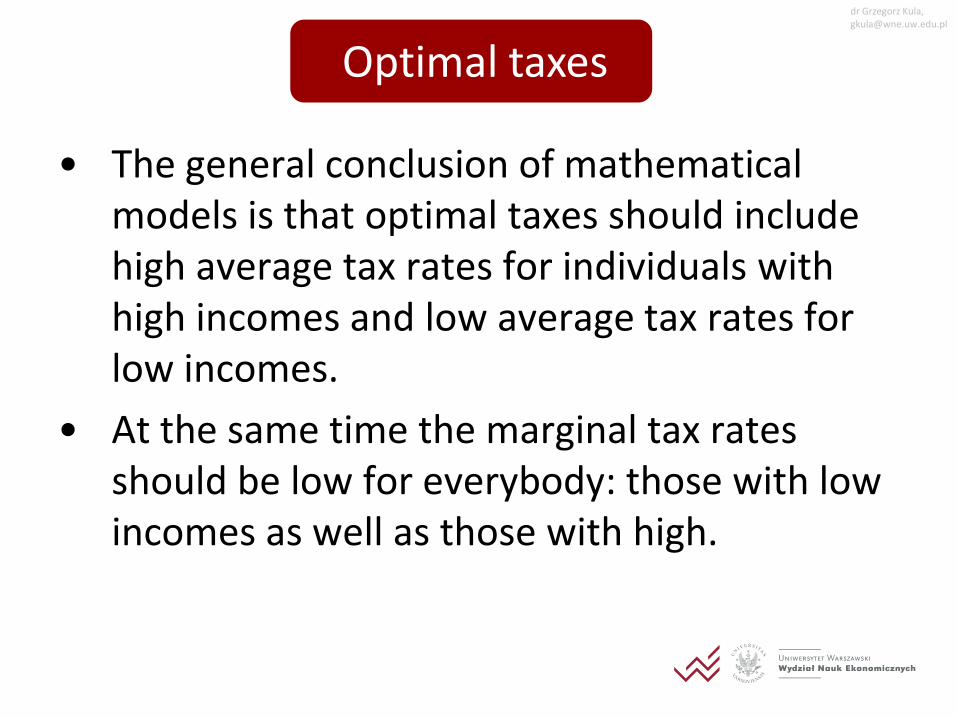
• The general conclusion of mathematical models is that optimal taxes should include high average tax rates for individuals with high incomes and low average tax rates for low incomes.
• At the same time the marginal tax rates should be low for everybody: those with low incomes as well as those with high.
Optimal taxes
dr Grzegorz Kula, [email protected]
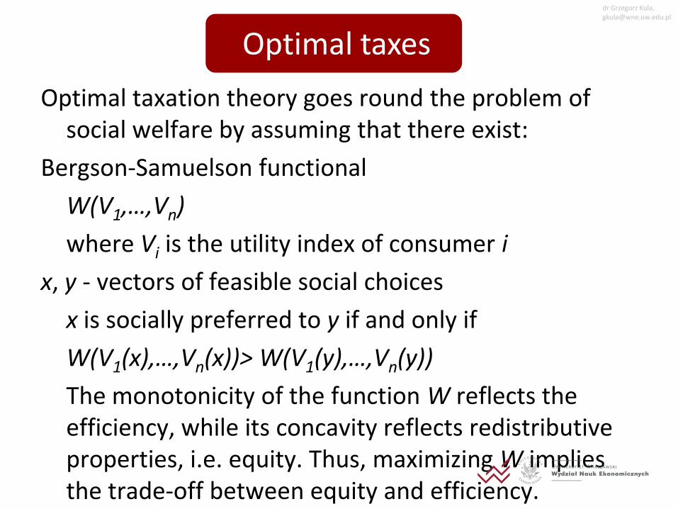
Optimal taxation theory goes round the problem of social welfare by assuming that there exist:
Bergson-Samuelson functional
W(V1,…,Vn)
where Vi is the utility index of consumer i
x, y - vectors of feasible social choices
x is socially preferred to y if and only if
W(V1(x),…,Vn(x))> W(V1(y),…,Vn(y))
The monotonicity of the function W reflects the efficiency, while its concavity reflects redistributive properties, i.e. equity. Thus, maximizing W implies the trade-off between equity and efficiency.
Optimal taxes
dr Grzegorz Kula, [email protected]
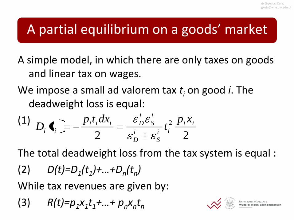
A partial equilibrium on a goods’ market
A simple model, in which there are only taxes on goods and linear tax on wages.
We impose a small ad valorem tax ti on good i. The deadweight loss is equal:
(1)
The total deadweight loss from the tax system is equal :
(2) D(t)=D1(t1)+…+Dn(tn)
While tax revenues are given by:
(3) R(t)=p1x1t1+…+ pnxntn
22
2 ii
ii
S
i
D
i
S
i
Diii
ii
xpt
dxtptD
dr Grzegorz Kula, [email protected]
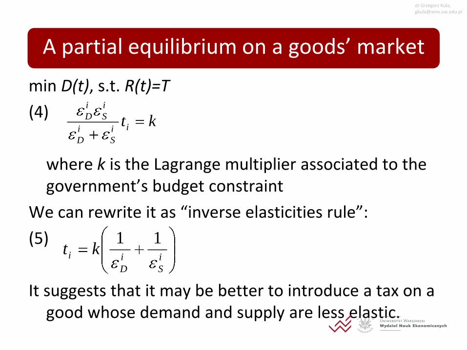
min D(t), s.t. R(t)=T
(4)
where k is the Lagrange multiplier associated to the government’s budget constraint
We can rewrite it as “inverse elasticities rule”:
(5)
It suggests that it may be better to introduce a tax on a good whose demand and supply are less elastic.
ktii
S
i
D
i
S
i
D
i
S
i
D
i kt11
A partial equilibrium on a goods’ market
dr Grzegorz Kula, [email protected]
Optimal taxation in general equilibrium model
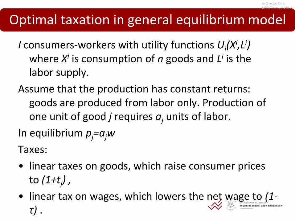
I consumers-workers with utility functions Ui(Xi,Li)
where Xi is consumption of n goods and Li is the labor supply.
Assume that the production has constant returns: goods are produced from labor only. Production of one unit of good j requires aj units of labor.
In equilibrium pj=ajw
Taxes:
• linear taxes on goods, which raise consumer prices to (1+tj) ,
• linear tax on wages, which lowers the net wage to (1-τ) .
dr Grzegorz Kula, [email protected]
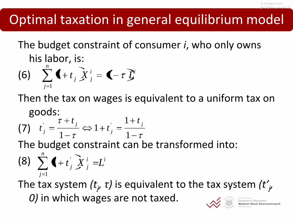
The budget constraint of consumer i, who only owns his labor, is:
(6)
Then the tax on wages is equivalent to a uniform tax on goods:
(7)
The budget constraint can be transformed into:
(8)
The tax system (tj, τ) is equivalent to the tax system (t’j, 0) in which wages are not taxed.
in
j
i
jj LXt1
11
1
11
1
'' j
j
j
j
tt
tt
in
j
i
jj LXt1
'1
Optimal taxation in general equilibrium model
dr Grzegorz Kula, [email protected]
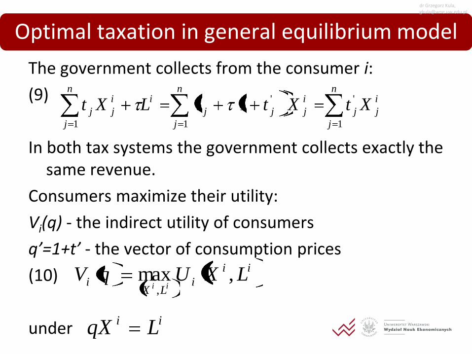
The government collects from the consumer i:
(9)
In both tax systems the government collects exactly the same revenue.
Consumers maximize their utility:
Vi(q) - the indirect utility of consumers
q’=1+t’ - the vector of consumption prices
(10)
under
n
j
i
jj
n
j
i
jjj
n
j
ii
jj XtXttLXt1
'
1
'
1
1
ii
iLX
i LXUqVii
,max,
ii LqX
Optimal taxation in general equilibrium model
dr Grzegorz Kula, [email protected]
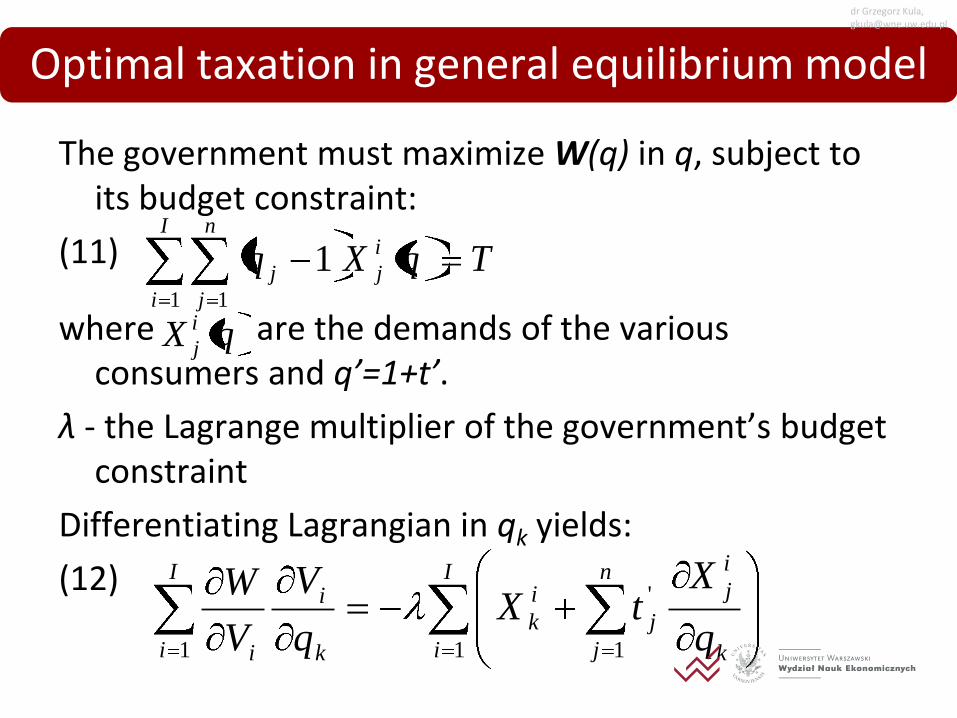
The government must maximize W(q) in q, subject to its budget constraint:
(11)
where are the demands of the various consumers and q’=1+t’.
λ - the Lagrange multiplier of the government’s budget constraint
Differentiating Lagrangian in qk yields:
(12)
I
i
n
j
i
jj TqXq1 1
1
I
i
I
i
n
j k
i
j
j
i
k
k
i
i q
XtX
q
V
V
W
1 1 1
'
Optimal taxation in general equilibrium model
qX i
j
dr Grzegorz Kula, [email protected]
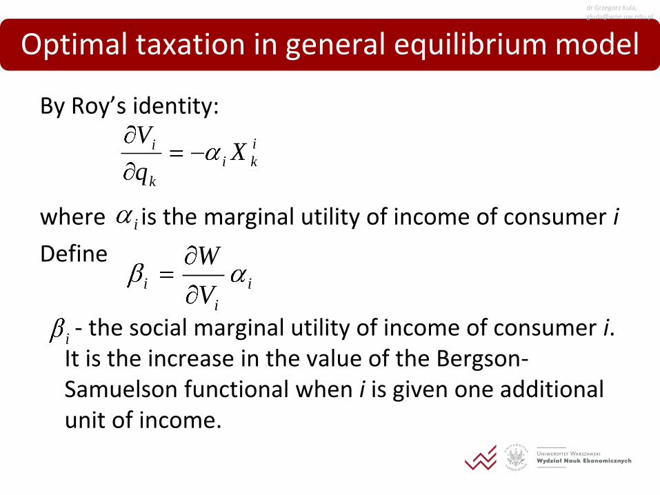
By Roy’s identity:
where is the marginal utility of income of consumer i
Define
- the social marginal utility of income of consumer i. It is the increase in the value of the Bergson-Samuelson functional when i is given one additional unit of income.
i
ki
k
i Xq
V
i
i
i
iV
W
i
Optimal taxation in general equilibrium model
dr Grzegorz Kula, [email protected]
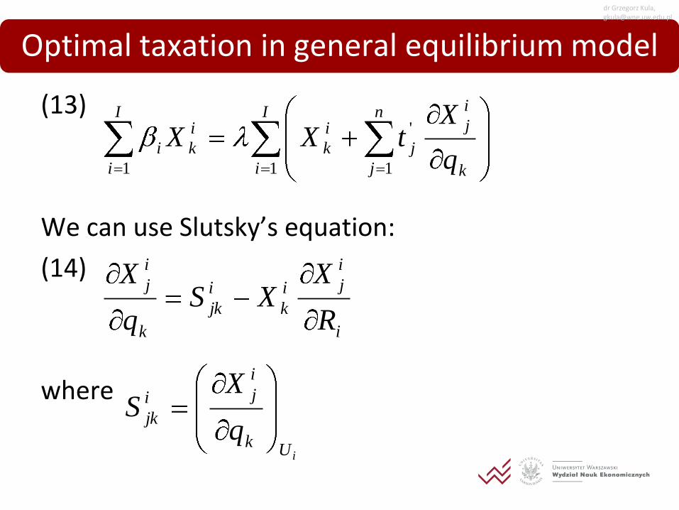
(13)
We can use Slutsky’s equation:
(14)
where
I
i
I
i
n
j k
i
j
j
i
k
i
kiq
XtXX
1 1 1
'
i
i
ji
k
i
jk
k
i
j
R
XXS
q
X
iUk
i
ji
jkq
XS
Optimal taxation in general equilibrium model
dr Grzegorz Kula, [email protected]
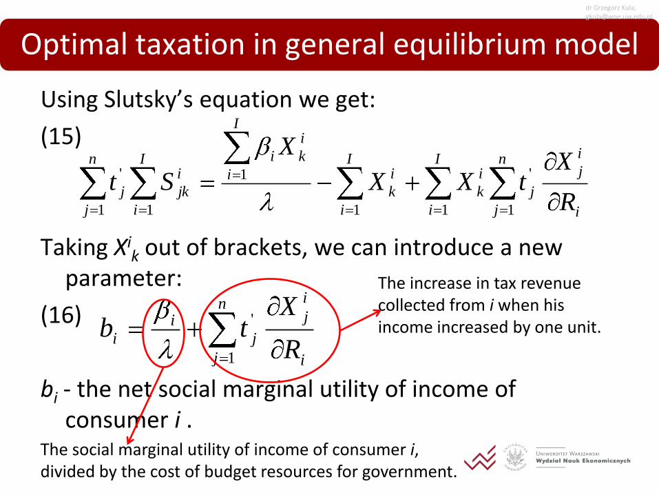
Using Slutsky’s equation we get:
(15)
Taking Xik out of brackets, we can introduce a new
parameter:
(16)
bi - the net social marginal utility of income of consumer i .
n
j i
i
j
j
I
i
i
k
I
i
i
k
n
j
I
i
i
kiI
i
i
jkjR
XtXX
X
St1
'
111
1
1
'
n
j i
i
j
ji
iR
Xtb
1
'
Optimal taxation in general equilibrium model
The social marginal utility of income of consumer i, divided by the cost of budget resources for government.
The increase in tax revenue collected from i when his income increased by one unit.
dr Grzegorz Kula, [email protected]
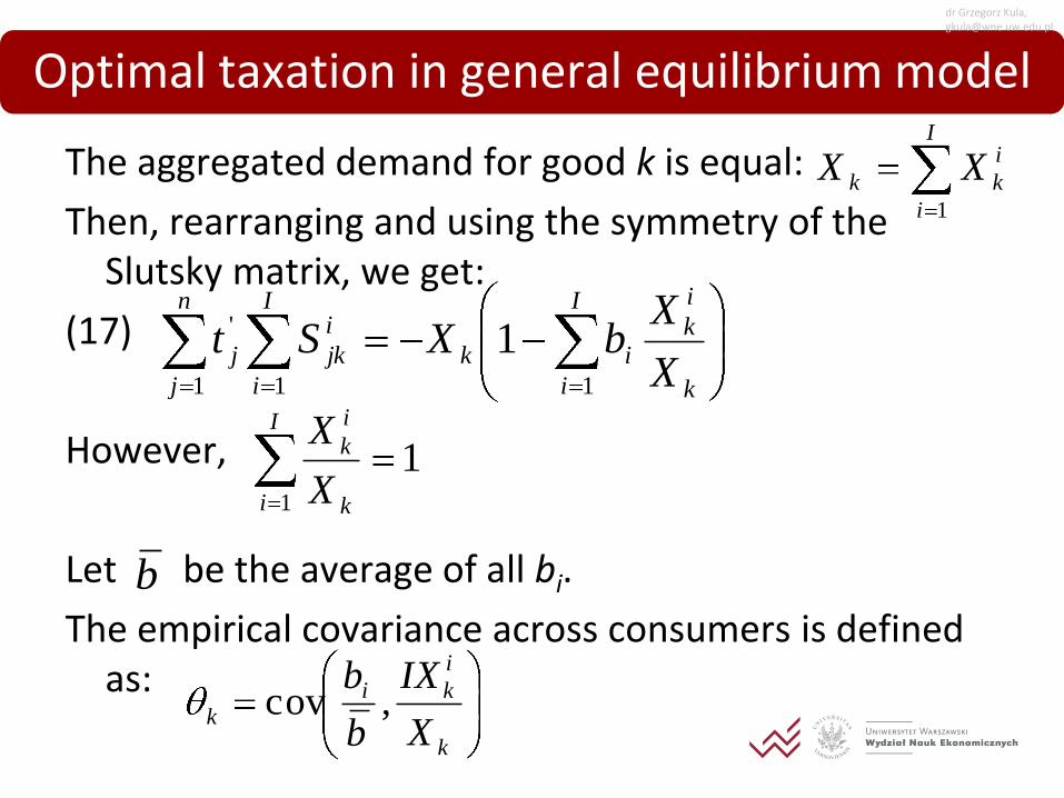
The aggregated demand for good k is equal:
Then, rearranging and using the symmetry of the Slutsky matrix, we get:
(17)
However,
Let be the average of all bi.
The empirical covariance across consumers is defined as:
I
i
i
kk XX1
k
i
kI
i
ik
n
j
I
i
i
jkjX
XbXSt
11 1
' 1
11
I
i k
i
k
X
X
b
k
i
kik
X
IX
b
b,cov
Optimal taxation in general equilibrium model
dr Grzegorz Kula, [email protected]
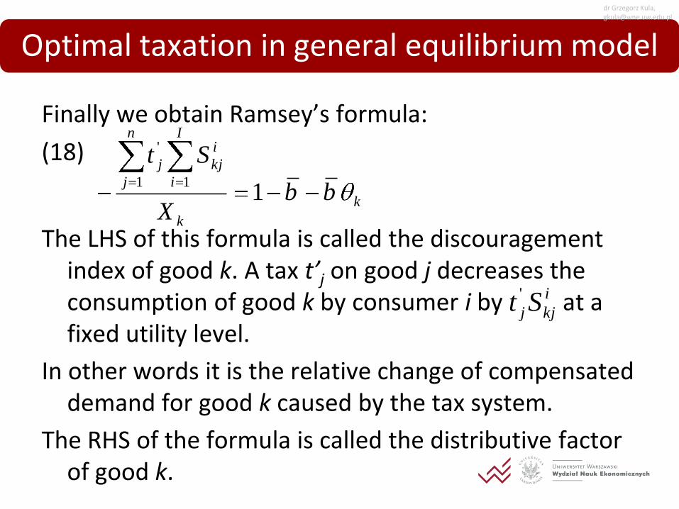
Finally we obtain Ramsey’s formula:
(18)
The LHS of this formula is called the discouragement index of good k. A tax t’j on good j decreases the consumption of good k by consumer i by at a fixed utility level.
In other words it is the relative change of compensated demand for good k caused by the tax system.
The RHS of the formula is called the distributive factor of good k.
k
k
I
i
i
kj
n
j
j
bbX
St
111
'
Optimal taxation in general equilibrium model
i
kjjSt '
dr Grzegorz Kula, [email protected]
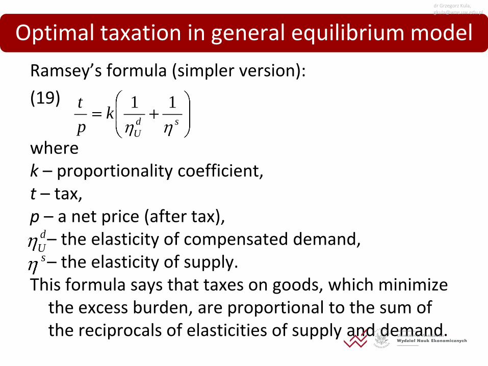
Ramsey’s formula (simpler version):
(19)
where k – proportionality coefficient, t – tax, p – a net price (after tax), – the elasticity of compensated demand, – the elasticity of supply. This formula says that taxes on goods, which minimize
the excess burden, are proportional to the sum of the reciprocals of elasticities of supply and demand.
sd
U
kp
t 11
d
Us
Optimal taxation in general equilibrium model
dr Grzegorz Kula, [email protected]
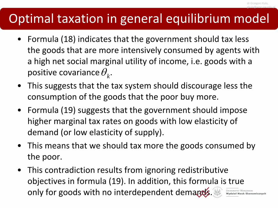
• Formula (18) indicates that the government should tax less the goods that are more intensively consumed by agents with a high net social marginal utility of income, i.e. goods with a positive covariance .
• This suggests that the tax system should discourage less the consumption of the goods that the poor buy more.
• Formula (19) suggests that the government should impose higher marginal tax rates on goods with low elasticity of demand (or low elasticity of supply).
• This means that we should tax more the goods consumed by the poor.
• This contradiction results from ignoring redistributive objectives in formula (19). In addition, this formula is true only for goods with no interdependent demands.
Optimal taxation in general equilibrium model
k
dr Grzegorz Kula, [email protected]
Optimal taxation of income (Mirrlees, 1971)
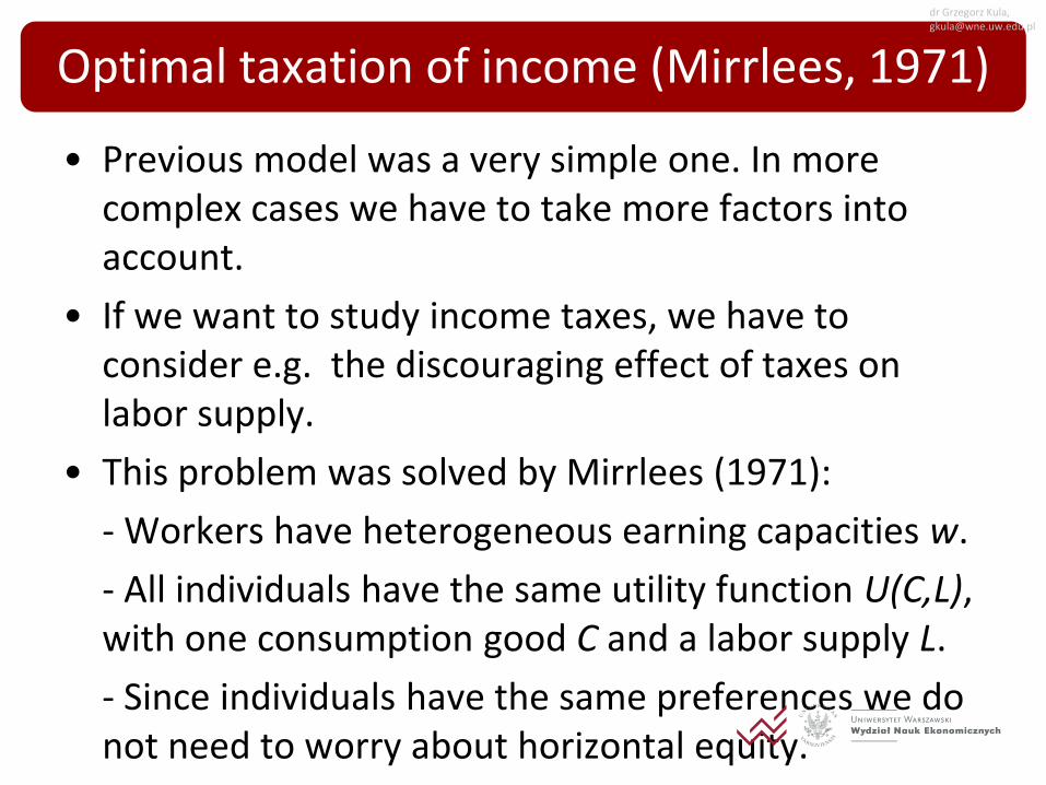
• Previous model was a very simple one. In more complex cases we have to take more factors into account.
• If we want to study income taxes, we have to consider e.g. the discouraging effect of taxes on labor supply.
• This problem was solved by Mirrlees (1971):
- Workers have heterogeneous earning capacities w.
- All individuals have the same utility function U(C,L), with one consumption good C and a labor supply L.
- Since individuals have the same preferences we do not need to worry about horizontal equity.
dr Grzegorz Kula, [email protected]
Optimal taxation of income (Mirrlees, 1971)
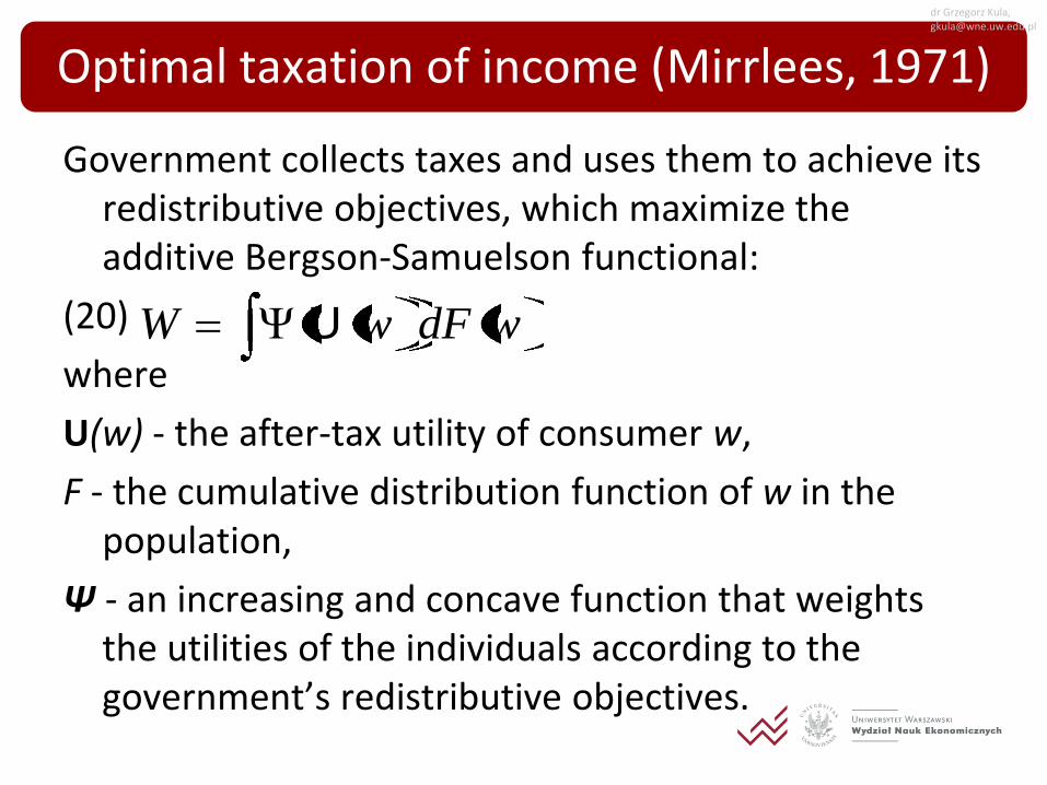
Government collects taxes and uses them to achieve its redistributive objectives, which maximize the additive Bergson-Samuelson functional:
(20)
where
U(w) - the after-tax utility of consumer w,
F - the cumulative distribution function of w in the population,
Ψ - an increasing and concave function that weights the utilities of the individuals according to the government’s redistributive objectives.
wdFwW UΨ
dr Grzegorz Kula, [email protected]
Optimal taxation of income (Mirrlees, 1971)
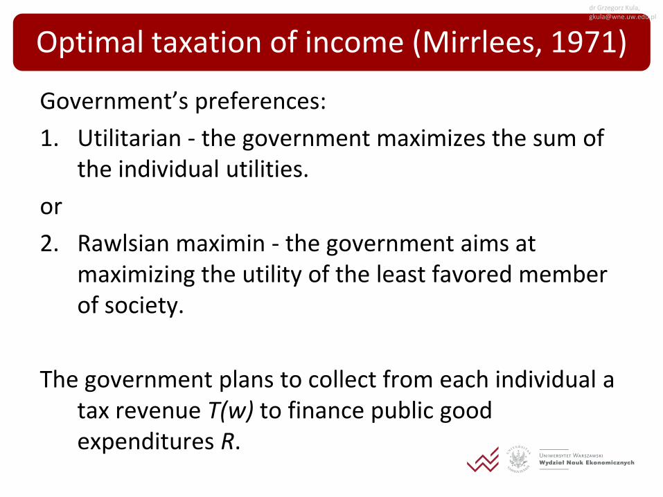
Government’s preferences:
1. Utilitarian - the government maximizes the sum of the individual utilities.
or
2. Rawlsian maximin - the government aims at maximizing the utility of the least favored member of society.
The government plans to collect from each individual a tax revenue T(w) to finance public good expenditures R.
dr Grzegorz Kula, [email protected]
Optimal taxation of income (Mirrlees, 1971)
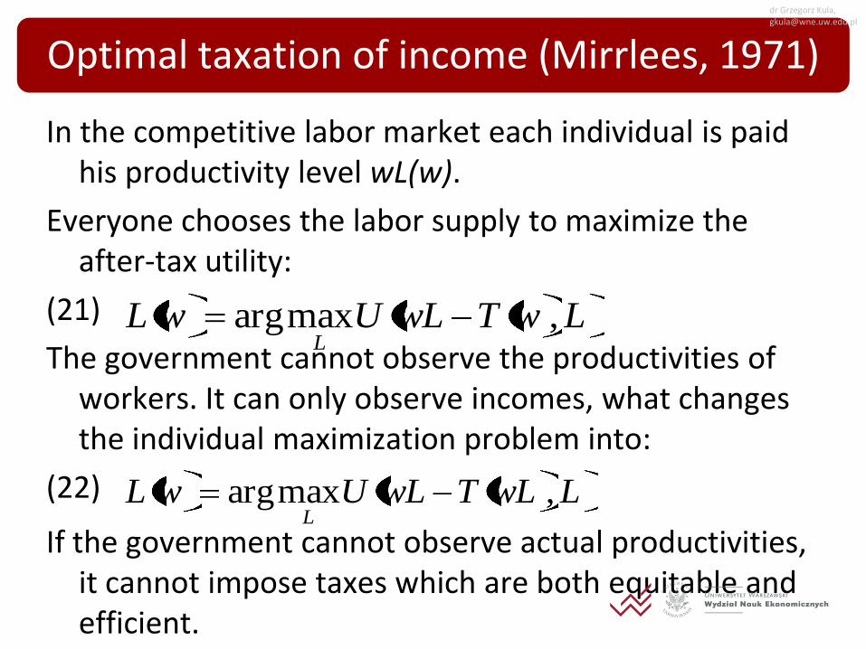
In the competitive labor market each individual is paid his productivity level wL(w).
Everyone chooses the labor supply to maximize the after-tax utility:
(21)
The government cannot observe the productivities of workers. It can only observe incomes, what changes the individual maximization problem into:
(22)
If the government cannot observe actual productivities, it cannot impose taxes which are both equitable and efficient.
LwTwLUwLL
,maxarg
LwLTwLUwLL
,maxarg
dr Grzegorz Kula, [email protected]
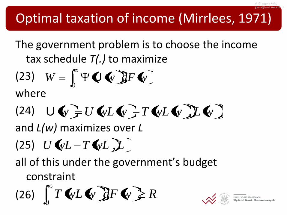
Optimal taxation of income (Mirrlees, 1971)
The government problem is to choose the income tax schedule T(.) to maximize
(23)
where
(24)
and L(w) maximizes over L
(25)
all of this under the government’s budget constraint
(26)
0wdFwW U
wLwwLTwwLUw ,U
LwLTwLU ,
0RwdFwwLT
dr Grzegorz Kula, [email protected]
1. Optimal taxation ignores many factors which are important for fiscal policy.
- The optimal taxation focuses on the vertical equity: taxes should be imposed subject to the taxpayers’ incomes and their abilities to gain income.
- Optimal taxes could be very difficult and expensive to collect and control, not mentioning the compliance costs for taxpayers.
Criticism of optimal taxation
dr Grzegorz Kula, [email protected]
2. Many solutions and conclusions of this theory can be reached in more intuitive way.
- Governments, while designing tax systems, do not build models based on Bergson-Samuelson functional.
- Any changes in tax systems are introduced slowly and gradually, with the objective to improve situation under Pareto optimality.
- If we have a nonlinear income tax, it is always possible to introduce tax reforms improving situation in Pareto sense.
Criticism of optimal taxation
dr Grzegorz Kula, [email protected]
3. The optimal taxes’ analysis does not give clear conclusions for the fiscal policy.
- Its results depend on the economic relations, which are difficult to study or measure in practice, and on information, which are not accessible.
- It is relatively easy to introduce a small change giving a Pareto improvement, but very difficult to run a complex reform of tax system.
- Often we cannot translate the results of optimal taxation models into precise, practical political actions.
Criticism of optimal taxation
dr Grzegorz Kula, [email protected]