Economics of Travel Demand Management: Comparative

Cost Effectiveness and Public Investment

BD 549-26

Final Report

March 2007

Economics of Travel Demand Management:

Comparative Cost Effectiveness and Public Investment

Final Report

March 2007

Prepared for

Florida Department of Transportation BD-549-26

Prepared by

National Center for Transit Research Center for Urban Transportation Research

University of South Florida 4202 E. Fowler Avenue, CUT 100

Tampa, FL 33620-5375 (813) 974-3120

http://www.nctr.usf.edu

The opinions, findings, and conclusions expressed in this publication are those of the authors and not necessarily those of the State of Florida Department of Transportation or

the US Department of Transportation

ii

1. Report No. NCTR 77704-00, FDOT BD549-26

2. Government Accession No.

3. Recipient's Catalog No.

5. Report Date March 2007

4. Title and Subtitle Economics of Travel Demand Management: Comparative Cost Effectiveness and Public Investment 6. Performing Organization Code

7. Author(s) Concas, Sisinnio, Winters, Philip L.

8. Performing Organization Report No.

10. Work Unit No. (TRAIS)

9. Performing Organization Name and Address Center for Urban Transportation Research 4202 E. Fowler Avenue, CUT 100 Tampa, FL 33620-57350

11. Contract or Grant No. DTRS98-G-0032 13. Type of Report and Period Covered

12. Sponsoring Agency Name and Address Office of Research and Special Programs Florida DOT U.S. Department of Transportation 605 Suwannee Washington, DC 20590 Tallahassee, FL 32399 14. Sponsoring Agency Code

15. Supplementary Notes Supported by a grant from the USDOT Research and Special Programs Administration, and the Florida Department of Transportation. 16. Abstract The 2006 Congestion Mitigation and Air Quality Improvement (CMAQ) Program Interim Guidance provides explicit guidelines to program effectiveness assessment and benchmarking by calling for a quantification of benefits, as well as disbenefits, resulting from emission reduction strategies for project selection and evaluation. The objective of this study is to develop a methodology that combines academic and practitioner experiences within a theoretical framework that truly captures consumers’ price responsiveness to diverse transportation options by embracing the most relevant trade-offs faced under income, modal price and availability constraints. The development of the theoretical model leads to the design and implementation of TRIMMS (Trip Reduction Impacts for Mobility Management Strategies), a practitioner oriented sketch planning tool. TRIMMS permits program managers and funding agencies like FDOT to make informed decisions on where to spend finite transportation dollars based on a full range of benefits and costs. The approach is consistent with other benefit to cost analyses. Its accuracy and the perceived fairness are critical when significant funds are at stake. The model allows some regions to use local data or opt to use defaults from national research findings, select the benefits and costs of interest, and calculate the costs and benefits of a given program. A step by step introduction to the program, its capabilities, and a set of working examples to guide the user through the process of evaluation is included in the report. A key strength of this model is its wide range of benefits and costs that can be selected for the analysis. The model’s flexibility and robustness allows it to be adopted by agencies throughout the country. Future research could seek to enhance the model to include more of the internal benefits to employers (e.g., changes in worker productivity, reduction in overhead, changes in employee retention, etc.). A byproduct of this research effort that goes beyond the initial project objectives is the development of a structured approach to evaluate the impact of soft programs. Compared to the currently available soft program evaluations methods, the approach developed this report provides a less heuristic method of estimation resulting in statistically robust mode share impact predictions. Another future area of analysis would be the refinement of such model to provide a standardized approach to soft program impact assessment. 17. Key Word Transportation Demand Management, TDM, Trip Reduction, Value of a Trip Removed, TDM Impacts, TDM Evaluation, TDM Benefits, TDM Comprehensive Evaluation, TRIMMS, Soft Programs

18. Distribution Statement

19. Security Classif. (of this report) Unclassified

20. Security Classif. (of this page) Unclassified

21. No. of Pages

80

22. Price

iii

Florida Department of Transportation Project Manager: Michael Wright, Commuter Assistance Program Manager Principal Investigators: Sisinnio Concas, Senior Research Associate Philip L. Winters, TDM Program Director Project Staff: Anurag Komanduri, Graduate Research Assistant Vishaka Shiva Raman, Graduate Research Assistant Liren Huago, Graduate Research Assistant

iv

Executive Summary The 2006 Congestion Mitigation and Air Quality Improvement (CMAQ) Program Interim Guidance provides explicit guidelines to program effectiveness assessment and benchmarking by calling for a quantification of benefits, as well as disbenefits resulting from emission reduction strategies for project selection and evaluation[1]. More public agencies are attempting to measure the value of Transportation Demand Management (TDM) strategies relative to their potential benefits and costs in comparison to other transportation solutions commonly employed to address capacity needs. Various tools, such as the Worksite Trip Reduction Model (WTRM) developed by the National Center for Transit Research, the Environmental Protection Agency (EPA) COMMUTER model, and impact calculation methods developed by the California Air Resources Board (CARB), are currently available for estimating some of the benefits of several TDM and other emission reduction strategies. However, no standardized guidance exists to quantify the costs and benefits of TDM strategies that considers the full range of benefits and costs accrued. The availability of an effective tool that takes into account a broader range of costs and benefits could greatly enhance agencies’ abilities to evaluate alternatives and estimate post-implementation benefits of TDM strategies. At the same time, poor estimates could steer traffic mitigation and emission reduction policies towards inefficient transportation investments at the local and regional level. The objective of this project is to develop a standardized methodology for calculating the costs and benefits of TDM for comparative assessment and public decision making. To achieve this goal, this report conceptualizes a new approach that builds on existing techniques and tools to produce a model that would save agencies time and money, providing a high level of reliability in impact estimates, while generating results that could be compared among regions and across projects. A methodology that combines academic and practitioner experiences within a theoretical framework that truly captures what is at the core of TDM evaluation is herein detailed. That is, an approach that models consumers’ price responsiveness to diverse transportation options by embracing the most relevant trade-offs faced under income, mode cost and availability constraints. The development of the theoretical model leads to the design and implementation of TRIMMS (Trip Reduction Impacts for Mobility Management Strategies), a practitioner oriented sketch planning tool. TRIMMS permits program managers and funding agencies like FDOT to make informed decisions on where to spend finite transportation dollars based on a full range of benefits and costs. The approach is consistent with other benefit to cost analyses. Its accuracy and the perceived fairness are critical when significant funds are at stake. The model allows some regions to use local data or opt to

v

use defaults from national research findings, select the benefits and costs of interest, and calculate the costs and benefits of a given program. A key strength of this model is its wide range of benefits and costs that can be selected for the analysis. The model’s flexibility and robustness allows it to be adopted by agencies throughout the country. A step by step introduction to the program, its capabilities, and a set of working examples to guide the user through the process of evaluation is included in the report. Future research could seek to enhance the model to include more of the internal benefits to employers (e.g., changes in worker productivity, reduction in overhead costs, changes in employee retention, etc.). The challenge of this future enhancement is finding data relating to given TDM strategies to such business outcomes. Another area of future research would be to develop a framework to include regional or local values for some of the cost externalities and mode price elasticities for region-specific analysis. Finally, a byproduct of this research effort that goes beyond the initial research objectives is the development of a structured approach to evaluate the impact of soft programs (i.e., programs other than changes in time or costs such as guaranteed ride home programs). Compared to the currently available soft program evaluation methods, the approach developed in this report provides a less heuristic method of estimation, resulting in statistically robust mode share impact predictions. Another future area of analysis would be the refinement of such a model to provide a standardized approach to soft program impact assessment.

vi

Table of Contents

Executive Summary ............................................................................................................ v

Introduction......................................................................................................................... 1

Current Systematic Evaluation Methods ............................................................................ 4

COMMUTER Model V2.0 ............................................................................................. 4 Advantages and Constraints........................................................................................ 6

International Evaluation Procedures ............................................................................... 8 New Zealand Transfund Theoretical Framework and Evaluation Procedure........... 11 Advantages and Constraints...................................................................................... 13

Other Existing General Guidelines to Evaluating Strategies........................................ 15 Case Studies ...................................................................................................................... 16

University of Washington U-Pass Program.................................................................. 16 Program Strategies .................................................................................................... 16 Program Evaluation .................................................................................................. 17

Way-To-Go, Seattle!..................................................................................................... 18 Program Strategies .................................................................................................... 19 Program Evaluation .................................................................................................. 19

Hayward “Heavy Up” Promotion Evaluation- San Francisco Bay Area Rapid Transit (BART) ......................................................................................................................... 22

Program Strategy ...................................................................................................... 23 Program Evaluation .................................................................................................. 23

AT&T Telework Program............................................................................................. 24 TDM Strategies......................................................................................................... 24 Program Evaluation .................................................................................................. 25

Evaluating Behavior Change in Transport: Benefit Cost Analysis of Individualized Marketing for the City of South Perth .......................................................................... 25

TDM Strategies......................................................................................................... 26 Program Evaluation .................................................................................................. 26

Trip Reduction Performance Program, Washington State............................................ 28 Proposed Prediction Model............................................................................................... 31

Modeling Technique ..................................................................................................... 33 Constant Elasticity Demand for Trips....................................................................... 33 Advantages and Constraints...................................................................................... 35 Soft Program Trip Change Adjustments................................................................... 36

Evaluation Criteria ........................................................................................................ 39 Evaluation Method: Per Passenger-Trip Average Annualized Benefits....................... 40

Applied Example: Transit Travel Time Improvement and Parking Cost Increase... 42 Model Implementation: TRIMMS.................................................................................... 47

Defining the Base Case: Input Requirements ........................................................... 49

vii

Soft Program Impacts ............................................................................................... 51 Model Output ............................................................................................................ 53 Customizing the Model............................................................................................. 55

Analysis Examples........................................................................................................ 59 Hard Program Impacts: Transit Fare Subsidy........................................................... 59 Soft and Hard Program Impacts................................................................................ 63

Conclusions....................................................................................................................... 70

References......................................................................................................................... 71

List of Tables Table 1 New Zealand Transfund TDM Benefits and Costs............................................. 11 Table 2 U-Pass Program Evaluation ................................................................................. 18 Table 3 Pollution Costs..................................................................................................... 22 Table 4 ROI of BART Promotional Campaign ................................................................ 24 Table 5 SOV Cost Externalities........................................................................................ 40 Table 6 Analysis Example Base Case Scenario Assumptions.......................................... 59

List of Figures Figure 1 EPA COMMUTER V 2.0 Estimating Procedure ................................................. 6 Figure 2 Model Flowchart ................................................................................................ 32 Figure 3 Demand for SOV trips........................................................................................ 44 Figure 4 TRIMMS – Inner Layout................................................................................... 48 Figure 5 TRIMMS – Base Case Scenario Worksheet ...................................................... 49 Figure 6 TRIMMS - Financial Incentive Worksheet........................................................ 50 Figure 7 TRIMMS – Travel Time Improvements Worksheet .......................................... 51 Figure 8 TRIMMS – Step by Step Soft Program Evaluation ........................................... 53 Figure 9 TRIMMS – Model Output.................................................................................. 54 Figure 10 TRIMMS – Model Parameters Modification ................................................... 56 Figure 11 TRIMMS – Price and Travel Time Elasticity Parameters Modification.......... 57 Figure 12 TRIMMS - User Supplied Final Mode Shares ................................................. 58 Figure 13 TRIMMS – Transit Fare Subsidy ..................................................................... 60 Figure 14 TRIMMS - Transit Fare Subsidy Impact......................................................... 60 Figure 15 TRIMMS – Transit Subsidy and Parking Surcharge........................................ 61 Figure 16 TRIMMS – Transit Subsidy and Parking Surcharge Impacts .......................... 62 Figure 17 TRIMMS – Transit Subsidy and Parking Surcharge Final Mode Share Impacts........................................................................................................................................... 62 Figure 18 TRIMMS – Soft Program Module: Step One.................................................. 63 Figure 19 TRIMMS – Soft Program Module: Step Two.................................................. 64 Figure 20 TRIMMS – Soft Program Module: Step Three................................................ 65 Figure 21 TRIMMS – Soft Program Module: Step Four.................................................. 66 Figure 22 TRIMMS – Soft Program Module: Step Five .................................................. 67 Figure 23 TRIMMS – Soft Program Module: Step Six.................................................... 68 Figure 24 TRIMMS Combined Hard Program/Soft Program Impacts............................. 69

viii

Introduction Transportation Demand Management (TDM) refers to the various strategies adopted to change travel behavior to increase the transportation system efficiency and also to achieve reduction in congestion, energy and fuel conservation, savings in parking and road costs, while focusing on the safety and mobility of the road users. The 2006 Congestion Mitigation and Air Quality Improvement (CMAQ) Improvement Program Interim Guidance provides explicit guidelines to program effectiveness assessment and benchmarking by calling for a quantification of benefits, as well as disbenefits resulting from emission reduction strategies for project selection and evaluation[1]. More public agencies are attempting to measure the value of TDM strategies relative to their potential benefits and costs in comparison to other transportation solutions commonly employed to address capacity needs. They seek to assess if the strategies have met performance-based planning standards or goals established for the strategies and whether or not it was a cost-effective expenditure of funds. For example, the Washington State Commute Trip Reduction program revealed that “the program’s cost to the state was 54¢ per reduced trip (or $136 for the year)[2].” These findings were used in some urban areas to argue for increased public funding to support employer TDM programs and provide incentives for the use of alternative modes. To date, no standardized guidance exists to quantify the costs and benefits of TDM strategies that takes into account the range of benefits and costs that accrue from TDM programs. The objective of this project is to develop a standardized methodology for calculating the costs and benefits of TDM for comparative assessment and public decision making. To achieve this goal, this report conceptualizes a new approach that builds on existing techniques and tools to produce a model that would save agencies time and money, would provide a high level of reliability in impacts results, while generating results that could be compared among regions and across projects. A methodology that combines academic and practitioner experiences within a theoretical framework that truly captures what is at the core of TDM evaluation is herein detailed. That is, an approach that models consumers’ price responsiveness to diverse transportation options by embracing the most relevant trade-offs faced under income, modal price and availability constraints. This report is divided into four main sections. Section I deals with systematic TDM evaluation methods. The analysis focuses on evaluation approaches that have a formal theoretical and empirical structure that result in tools for program benefits estimation. Each of the methods’ advantages and constraints are discussed to highlight key elements for evaluation and inclusion in the model development phase.

1

The investigation involved a comprehensive search of transportation databases and Internet sources to ensure comprehensive coverage of reports and papers describing relevant aspects of TDM assessment. In addition, CUTR reached out to nearly 1,000 subscribers in its TRANSP-TDM listserv to identify evaluation and return on investment analyses. The review uncovered a paucity of predictive evaluation approaches to TDM program evaluation and cost effectiveness. Most of the evaluation experience in the U.S. is based on the assessment of individual pilot projects and programs that focus on single TDM measures (such as vanpooling or user subsidies) or on employer sites. Broader evaluations are conducted on a cross-sectional basis over a range of multi-objective programs[3]. The most relevant predictive evaluation methods and models are represented by the Environmental Protection Agency (EPA) COMMUTER model and by the New Zealand and Australian experiences[4-6]. The remaining models are in the form of business benefits calculators, which are mainly designed to aid employers and practitioners in setting up specific TDM programs. In addition, the review of international experiences dealt with a detailed analysis of manuals and guidelines to TDM program evaluation and effectiveness. These studies provide details and general direction towards a more comprehensive approach to TDM assessment in a fashion similar to that currently employed in the evaluation of transportation infrastructure investments. The bulk of this work has been compiled by the research conducted by the Victoria Transport Policy Institute, based in Canada[7-10]. Section II of the report reviews a set of case studies spanning diverse TDM strategies. The objective is to assess how programs are evaluated, what measures of impacts and assessment are employed, and how these measures vary according to the TDM strategy being assessed. The literature search uncovered a host of case studies. This section focuses on those that are most relevant to this study’s objectives. This section also includes a review of the Commute Trip Reduction Performance Grant Program of Washington State Department of Transportation. Although not related to a specific TDM program or implementation, this case study review was deemed as relevant because it offers an innovative approach to assessing the value of TDM by introducing the market-based concept where buyers and sellers compete to determine the price of a removed single occupancy vehicle (SOV) trip. Section III provides the rationale for seeking an alternative method to evaluate TDM strategies on a more comprehensive basis. The analysis carried out in Section I and the methods currently in use and described in Section II provide the basis for looking to develop a standard approach to TDM evaluation that overcomes the constraints outlined in this report. This section details a methodology that combines academic and practitioner experiences to produce a theoretical framework that truly captures what is at the basis of TDM travel behavior: an approach that models consumers’ price responsiveness to diverse transportation options by embracing the most relevant trade-offs faced under income, modal price and availability constraints. The development of the theoretical model leads to the design and implementation of a sketch planning tool, TRIMMS (Trip Reduction Impacts for Mobility Management Strategies) and is detailed in Section IV. The section provides a step by step introduction

2

to the program, its capabilities, and a set of working examples to guide the user through the process of evaluation. The work concludes with recommendations on how to improve and expand the model and provides direction for further research.

3

Current Systematic Evaluation Methods This section is concerned with models that evaluate TDM cost effectiveness for public funding purposes. They provide formal ways to model the impacts of TDM alternatives in a predictive fashion. The ensuing literature review focuses on methods incorporating (1) costs and benefits in economic terms accompanied by (2) a calculator or estimator or “model” for projecting TDM effects of one or more TDM strategies being considered for implementation. The literature search uncovered few existing approaches to the evaluation of TDM impacts on a predictive basis. To date, most of the evaluation deals with the assessment of individual pilot projects and programs that focus on single TDM measures (such as vanpooling or user subsidies) or on employer sites[3]. The vast majority of these methods take the form of calculators for the set up and benefits assessment of employer-based programs. Usually, such tools are not predictive in nature, or if so, they tend to be based on simple rule-of-thumb approaches. The review showed that the most common evaluation method is cost benefit analysis, as it provides both a means of recommending and ranking different alternatives. The constraints associated with these approaches are related to the necessary estimation of each of the identified benefits and costs, and the difficulty to provide a comprehensive evaluation of concurrent TDM strategies (i.e., synergistic effects). These approaches are characterized by a structured approach to the quantification of benefits, such as travel time savings, congestion reduction, health and fitness. The methods provide ways to estimate the change in benefits brought about by different TDM strategies, as well as monetary values. The latter are usually provided in ranges and are the byproduct of current and past studies at an aggregate level.

COMMUTER Model V2.0 The COMMUTER model, developed by the Environmental Protection Agency, is intended to be used to project emission impacts of different TDM strategies of commuter choice incentive programs. The model is capable of estimating, at a sketch planning level, impacts of TDM strategies directed at affecting accessibility, transit time, walking time, parking pricing, modal and other subsidies[7, 8]. The impacts of alternative TDM strategies are estimated differently according to the program being considered, as shown in Figure 1. For example, impacts of “soft programs,” such as alternative work schedules and employer support programs are projected by means of look-up tables. These look-up tables provide modal incremental changes that are associated with the programs being considered, reflecting different application assumptions and levels of intensity. A normalization procedure assures that total mode share sums to 100 percent.

4

TDM strategies that impact travel costs and travel times are estimated using pivot point logit model approach. This consists of a simplified version of the traditional four-step travel demand forecasting procedure to estimate changes in vehicle miles traveled (VMT) and the related number of trips spanning from generalized cost and travel time changes. At the core of the model is the following basic pivot point logit equation:

( )i

m

UUUU

U

eeeeemP

++++=

...321

Where ( )mP = share of mode m;

e = exponential function; mU = utility equation for mode m; and,

iU ...1 = utility of other alternative modes It is then sufficient to use the above equation to enter the initial or base mode share, mode use ad-hoc or default parameters entering each mode’s utility function to obtain the projected change in modal share due, for example, to a change in generalized cost. The modal share is produced by TDM programs or projects that change the cost or time costs across modes. The model estimates and reports the following:

• Baseline and final mode share by mode, including percent of trips eliminated; • Percent of trips shifted by peak period; • Change in VMT (based on trips removed multiplied by percentage of workforce

affected and average trip length); and, as a result of the change in VMT, • Total daily emission reduction for each pollutant.

5

Figure 1 EPA COMMUTER V 2.0 Estimating Procedure

Source: COMMUTER V 2.0 Procedure Manual

Advantages and Constraints The major advantages of the COMMUTER model are its simplicity and the required level of aggregation. For example, the model differentiates between three basic categories of metropolitan areas from 750,000 to over two million people; has two scopes of analysis (regional and on-site), and accounts for three urban area types (central Business District, high density activity center, and suburban low density areas). The

6

aggregation of results is justified by assuming that TDM programs generate modest modal changes providing an acceptable trade-off between accuracy and ease of use. The pivot logit equation approach simplifies the estimation process and drastically reduces data requirements, making the model available to a broader, less technically oriented, audience of planners and employers. Coefficients derived from regional or area specific travel demand models are used as inputs and applied to the pivot logit equation to estimate changes in baseline mode shares spurred from specific TDM strategies. The coefficients are assumed to be derived using sound statistical methods to guarantee statistical robustness. Among the constraints of such an approach are:

• Trips and VMT estimates are strongly dependent on pre-specified parameters; • No guarantee that the pivot logit equation will predict actual mode shift (predicted

mode shift will lie on the logit curve); • The logit equation is based on discrete, mutually exclusive choices (auto vs.

transit, without admitting concurrent choices of transit and, say, walking); • Coefficients are affected by factors such as the variables included in the model

(and the interactions between the variables), calibration procedures, and the quality of the underlying data; and,

• There is no distinction between short run vs. long run effects. The default parameters are obtained from traditional four-step travel demand forecast models. These models are usually estimated and calibrated for specific regions and uses, with little potential for a generalized use, transferability across different regional areas, and predictive power. This is more evident when trying to estimate the impact of TDM strategies in areas where regional transport demand models are not available.1 The trade-off of using pivot-point modeling versus more intensive computational methods, like four-step travel demand forecasting model is justified by assuming that for modest change in mode shares, such as those generated by TDM strategies, the incremental extrapolation is fairly accurate. The COMMUTER procedure manual suggests that there exist other ways of applying the incremental or pivot-point modeling approach, for example by applying elasticity parameters from empirical work to extrapolate changes in base values. The use of elasticities was not considered as it was argued that they are “limited in being able to take into account the interactive effects that occur when multiple actions are applied or multiple modes are evaluated.[8]” This assertion, though, seems to contradict the preferred choice of the pivot-point logit approach. Indeed, the logit equation is based on a multinomial discrete choice model, which by its own definition estimates the likelihood that different, mutually exclusive choices are simultaneously taken by an individual. The 1 The user manual that accompanies the Commuter model reports that travel and emission impact estimates are “highly sensitive to the values of these coefficients, especially cost coefficients.” The user is warned against creating hybrid equations or altering the default parameters in the absence of detailed local data from travel forecasting models.

7

use of elasticities in a properly tailored framework could take into account direct and indirect relationships between different modes. In addition, the use of cross elasticities assures taking into account substitution and complementary effects among transportation alternatives. Finally, the use of the pivot-point logit equation precludes the distinction between short run and long run effects. The parameters that influence modal shares are the byproduct of cross-sectional analyses (unless specified otherwise) which do not take into account the long-run adjustments those users inevitably face. The use of a model based on transport elasticities could provide a method that differentiates between a program’s short and long run impacts.

International Evaluation Procedures The literature review extended to cover models and approaches followed internationally, with a focus on predictive evaluation methods. European efforts are concentrated on monitoring and evaluation, as distinct from projection and estimation, with the biggest effort represented by the Mobility Management Strategies for the Next Decades (MOST). This project, sponsored by the European Commission until 2002, was intended to provide an insight on policy frameworks and implementation strategies, as well as an investigation of setting up standardized monitoring and evaluation tools[9]. The literature review did not encounter examples of predictive evaluations in Europe. Given the MOST project objectives and focus on monitoring and implementation, a full review of its structure and conclusions was omitted from this literature review.2 In addition, CUTR recently published a research effort summarizing European experiences in the field of TDM[10]. The bulk of international, non-European experience is reflected in the Australian and New Zealand efforts to develop predictive TDM evaluation procedures[5, 6]. In Australia and New Zealand most of the TDM measures fall under the definition of Travel Behavior Change (TBhC) strategies. TBhC embraces a subset of TDM measures mostly centered on marketing approaches designed to build awareness in SOV users about alternative modes of transports or to promote voluntary mode change. TBhC measures include:

• Workplace based initiatives (carpooling, vanpooling) • Telecommuting • School travel initiatives • Household initiatives • Community-based initiatives

2 Note: the Transfund literature review reported the unavailability of examples of predictive evaluations in UK and Europe or any established TDM evaluation procedures.

8

In New Zealand, evaluation of TDM strategies falls under the Transfund Funding Framework and Evaluation Procedures. A major requirement in the assessment is that TDM projections must be conducted using methods comparable to those used to assess traditional transportation infrastructure projects. The economic evaluation approach must be based on changes “in the perceived cost/benefits, with addition of resource cost correction and externality effects[5].” In addition, TDM projects are expected to produce benefits similar to those of road infrastructure projects and should be estimated using the same benefit and cost unit values, as provided by the Project Evaluation Manual (PEM). TDM projects should also be assessed with methods consistent with those developed for public transport and freight projects that contribute to reduced infrastructure and maintenance costs. The procedure takes into account the benefits added to existing users, the net benefits accruing to those switching modes as a result of the projects, and indirect benefits to the remaining users and environmental benefits. Under these guidelines, New Zealand Transfund commissioned a 2004 study to develop project assessment procedures suitable to TDM projects[6]. The study provides a comprehensive approach based on a cost/benefit analysis that includes the following three major benefit categories:3

• Benefit to traveler switching mode(s); • Resource cost corrections; and, • Externality benefits.

The premise to the approach is that the mode share of one mode with respect to another is “a function of the difference in generalized cost between the two modes.” This relationship is then used to determine the change in generalized cost to bring about the observed change in mode share. Conceptually, the approach follows that of EPA COMMUTER Model v2.0, as it relies on travel demand forecast models to obtain evaluation parameters. Contrary to the EPA model, which uses a relative mode share change, this approach uses an absolute percentage point change as reference parameters. The use of this approach “does not require any prior knowledge of initial mode share within a company, school or community.” This measure of benefit comprises the following categories of benefits:

• Travel time for new users; • Decongestion; • Induced traffic; • Vehicle operating costs; and,

3 Ultimately, the estimated benefit value for TDM users is $1.00 for each four percentage point change in mode share from SOV to public transport or cycle and walk.

9

• Safety. Table 1 reports the benefits considered, as well as ranges used as standard predictive evaluation measures. The study also recommends a range of diversion rates obtained from diverse projects located in Australia, New Zealand and worldwide. These rates are to be used as default values providing the expected changes in mode share from SOV to alternative modes, expressed as absolute percentage points. According to the report, these values “can be used without knowledge of existing mode shares,” which simplifies the approach, although it probably weakens the assessment. The diversion rates are estimated for different travel plans (school, work) in an aggregate fashion, without sub-grouping by location and socio-economic characteristics, due to unavailability of statistically significant coefficients.

10

Measure Description

Travel Time Savings Fully internalized and estimated by means of perceived benefit approach. These benefits comprise travel time difference between modes, waiting time, and trip time reliability

Resource cost with the following correction: half are internalhalf are included in net benefits to TDM userswalking benefits are 2.5 times of cycling

Resource cost with cost corrections that includes:car parking costland use costparking facility capital costssecurity costsResource cost correction assumption:car users perceive 75% of total resource cost

Considered as an externality. Resource cost with cost corrections. The corrections are:

vehicle operating cost savings equal to 7% of total travel time decongestion benefitsDiscount the effect of induced travel demand of TDM strategy using a 50% factor

Note: road system benefits are negligible and do not enter into cost correction ad additional benefit

Cycle Operating Costs Resource cost with cost corrections. The corrections is set to zero when accounting for additional accident risks by assuming increasing traffic calming effects

Walking Costs Same as cyclingResource cost with cost corrections, comprised of three parts:

1 - Internal perceived costs (to TDM user);2 - Internal costs not perceived with cost corrections3 - Externality cost born by society (hospital, loss productivity)

Note: Internal perceived cost savings are equal to 50-66% of accident resource costs

Public Transport Operating Cost Only included as a cost if the TDM strategy results in an increase in demand high enough to warrant additional infrastructure or operating costs

Environmental Externalities Estimated as the sum of all effects including local air, noise, and water pollution, and greenhouse gas emissions. These benefits enter only in short-run evaluations

Public Transport Fares

Vehicle Operating Costs

Resource cost with cost corrections. Part of the costs is directly perceived by users, such as fuel costs. Additional costs, such as vehicle operating, and other costs usually considered as fixed are included as a result of a TDM strategy that builds aw

Accident Costs – Car

Health Benefits of Cycling and Walking

Resource cost with cost corrections. Fares are a financial transfer from users to operators, but perceived as a cost by users.

Congestion Reduction

Car Parking

Table 1 New Zealand Transfund TDM Benefits and Costs

New Zealand Transfund Theoretical Framework and Evaluation Procedure The overall rationale for developing the Transfund evaluation approach to TDM is to justify funding sustainability while providing an evaluation framework consistent with what was used to evaluate highway and transit projects. The evaluation approach is based on a cost benefit analysis framework to allow a comparison with other types of

11

transport improvement interventions and to maintain credibility of TDM strategies and funding sustainability. The cost benefit analysis is based on a method that assesses changes in perceived costs which includes resource cost corrections. The general assumption is that travelers perceive only the direct costs related to a given transportation choice. These costs usually include out of pocket costs such as fuel, parking charges, and public transit fares. Fully perceived costs include the value of time (transit and waiting) and other externalities. The Transfund approach argues that in many cases the out-of-pocket costs do not fully account for the resource costs, hence resource cost corrections are needed. The resource cost corrections included in the assessment expand the range of out of pocket costs to include those initially unperceived costs uncovered to the user as a results of a TDM strategy. The framework takes into account the following benefits:

A. Resource benefits to people already using the mode which is improved (generalized cost change for that mode); this is especially important when studying the effect of transit improvements;

B. Perceived benefits to mode switchers (people changing behavior); C. Benefits from avoidance of unperceived costs associated with previous behavior

of switchers, comprising: 1. Resource cost adjustments for switchers themselves; including monetary

(e.g., non-fuel variable vehicle operating costs) and non-monetary (e.g., accident trauma); and,

2. Other resource cost impacts (externalities) on other transport system users or of the transport system (e.g., decongestion, environmental, and accident externalities).

D. Unperceived costs associated with new behavior of switchers, comprising:

i. Resource cost adjustments for switchers themselves; including monetary (e.g., public transport fare payments) and non-monetary (e.g., health benefits of cycling and walking); and,

ii. Other resource cost impacts (externalities) on other transport system users or on the transport system, e.g., environmental, accident, and health externalities (to the extent that costs of diminishing health were being incurred by society as a whole rather than the behavior changer individually).

Benefits of Type A are determined by changes in generalized costs (including time and comfort) to the existing users. Benefits of Type B are the most relevant in evaluating the impact of TDM strategies that influence the existing cost differentials among available modes. These strategies include

12

changes in vanpooling schedules or transit fare subsidies, and any other type of intervention that changes the total cost of transport of a given mode. Following consumer surplus theory, these benefits are calculated using the rule of one half of the benefits of Type A for existing users. For the evaluation of user benefits spanning from changes in perceived costs, the Transfund model relies on projected mode share changes as estimated by regional four-stage travel demand models. In this context, it is necessary to input the current modal share, as well as the expected modal share to estimate the required generalized cost changes to achieve a given goal. The report provides diversion rate tables that were then used as default values for predictive evaluation within a Microsoft Excel spreadsheet tool.4 The model evaluation results in a benefit to cost ratio that is then used as the “value for money” of TDM projects, which comprises:

• Net perceived and indirect benefits (and disbenefits) to all TDM users, other transport users affected by the project and all externalities. These elements constitute the numerator; and,

• Net costs to the government of the TDM strategy being evaluated, which constitutes the denominator.

Advantages and Constraints One of the major advantages of this approach is that it seeks to establish a methodology to provide a comprehensive assessment of the full range of benefits and costs brought about by TDM initiatives while maintaining a framework within the guidelines of the more traditional infrastructure investment appraisal. By following a perceived cost approach, TDM strategies are fully accounted for their impacts on internalizing costs that would be otherwise left out of the decision making process of TDM switchers. At the same time, the approach retains the theoretical construct of the more traditional benefit cost analysis. Two major constraints were identified in the Transfund approach to evaluate TDM strategies. The first deals with the way benefits are measured, due to the notions of resource costs and cost corrections. The approach is based on perceived costs whereas it is assumed that individuals face the full cost of the alternative chosen. For example, parking costs are assumed to comprise not only the average cost of parking, but the full opportunity cost of using land for parking, the capital cost of the parking infrastructure, and the cost of added security (if any) to the parking facility. Summed all together, these components represent the full resource cost of parking. A resource cost correction is then accounted for, by assuming that the individual internalizes only a percentage of the total 4 The evaluation procedure was formalized into a Microsoft Excel spreadsheet model now being used by the Victoria Travel Smart Program. Essentially, it is the same spreadsheet, but with values tailored to the Australian network.

13

resource costs. For example, in the case of parking resource costs, the model assumes that individual perceives 75 percent of the resource costs, with a required cost correction of 25 percent. A given TDM strategy might influence the way a user perceives this cost by either increasing or lowering the perceived component. By letting the researcher establish what should be included in perceived costs, and by assuming what individuals are able to internalize in terms of costs, the approach is likely to overestimate TDM benefits.5

Second, the model does not rely on a pivot point formula, but on a set of pre-estimated modal shares tailored for New Zealand. These shares are obtained from regional transport demand models and used as fixed parameters in the spreadsheet, without calling out a pivot logit or any equation. As in the case of the EPA COMMUTER model, the reliability of the modal share shifts relies upon regional estimates coming from traditional four-step models. As a result, the default parameters depend on the calibration processes employed in these models, which cannot be easily generalized in a broader context.

5 For example, the model assumes a full resource cost of parking of $10.00 for the Auckland area for peak period commuting trips to the Central Business District (CBD). Then, it assumes that individuals only perceive 75 percent of such cost for a total of $7.50. On the other hand, the average parking fee is only $2.50 (page 29). Another example is provided by how walking and cycling accident costs. When computing the total health benefits of walking and cycling, the model assumes that these are resource costs that do not need to be discounted by the risk of incurring in accidents (e.g., individuals do not internalize the added risk of switching to walking or cycling).

14

Other Existing General Guidelines to Evaluating Strategies The literature review revealed a substantial effort to uncover benefits brought about by TDM initiatives. There exist numerous practitioner oriented guidelines to TDM impact assessment based on formalized approaches to comprehensive evaluation[11-16]. Several studies have culled findings of program evaluations to compare the empirical evidence of a range of TDM alternatives[16, 17]. Some of the guidelines list relevant impact measures to evaluate TDM projects[11, 12, 18], and outline the major constraints to a comprehensive TDM evaluation. These research efforts all recognize that, generally, TDM projects result in relatively small impacts over a large number of individuals. They are more difficult to evaluate for the following reasons:

1. Impacts are different across users, whereas in project infrastructure evaluations users are assumed homogeneous (i.e., they receive the same benefits); and,

2. Different TDM strategies are simultaneously implemented calling for a comprehensive evaluation.

This leads to a trade-off between evaluation procedures that estimate all of the individual responses to TDM strategies and procedures that provide a more aggregate appraisal using a greater level of approximation. The approximation is an inevitable trade-off of the requirement of a standardized approach. These issues have been considered in the literature. TDM measures are social plans and their benefits encompass a vast sphere of social life. For example, a congestion reduction program might benefit not only from reductions in VMT, but might also gain from air quality improvements, decreased fossil fuel consumption, and reduced parking demand. Price changes can have a variety of impacts on travel, affecting the number of trips people take, their destination, route, mode, travel time, type of vehicle (including size, fuel efficiency and fuel type), parking location and duration, and which type of transport services they choose. All these are essential indicators in evaluating a TDM project. Approaches that are currently available to evaluate the cost effectiveness of TDM programs and strategies deal with assessing the impacts on a comparative basis[3]. This is usually carried out by assessing TDM impacts in terms of measures linked to emission reduction, such as vehicle trip or VMT reduction. To date, the bulk of work on measuring the effectiveness of TDM programs on a comparative basis in terms of emission reduction is represented by the Transportation Research Board Special Report 264[19]. This research effort summarized seminal work conducted to date with a focus on the cost effectiveness of programs funded under the objective of pollution emission reduction.

15

Case Studies In this section, a selected number of cases are presented, comprising studies that evaluate different popular TDM strategies. The objective is to provide insight on how TDM impacts are being quantified by practitioners, in particular:

• Evaluation Criteria – While general guidelines as provided by TDM expert publications provide a full range of benefits, practitioner experience provides additional insightful information as to what is actually measurable, given data and budgetary constraints; and,

• Evaluation Methods – Practitioner work can shed some light on the most

commonly used evaluation approaches, such as benefit cost, life cycle or least cost planning analyses.

As part of this section of the literature review, many reports were carefully perused. Each study that has been included in this report provides a different evaluation methodology and set of evaluation measures. Among the evaluation methods are return on investment analysis, break-even point analysis, and quantitative analysis focusing on advantages in a single sphere (e.g., travel times, air quality etc.), mathematical model evaluation and research oriented studies from Washington and Australia.

University of Washington U-Pass Program The U-Pass program was started by the University of Washington to offer flexible transportation to its students at a low price. Research for a new Campus Master Plan conducted by the University in 1989 projected an increase in the number of students, faculty and staff with a subsequent reduction in the number of parking spaces. The University thus assembled a task force of students, faculty and staff from two local transit agencies, namely the King County Metro and the Community Transit, and developed a new Transportation Master Plan (TMP). The key element of the plan was to significantly increase the University parking rates, to discourage driving alone and also to raise funds for the implementation of the U-Pass Program. With the above views, the program was launched in September 1991[20].

Program Strategies The key element of the U-Pass program is managing the demand of SOV through product pricing. It is an award winning program used as a model for other transportation programs, both locally and nationally. As the main idea of the U-Pass program is to encourage the students and staff to adopt alternative modes to driving alone, the participants are provided with many incentives including:

16

• Increased and subsidized transit service; • Ride matching services; • Vanpool subsidies; • Free carpool and vanpool parking; • Bicycle incentives; • Reimbursed rides home for emergencies; • Occasional parking permits for those who do not drive every day; • Night-time neighborhood shuttle service; and, • Merchant discounts.

In addition there are incentives offered on bicycle and pedestrian safety equipment, an emergency ride home program for employees, discounts on Flexcar, etc. All these measures have helped in reducing the number of people traveling by SOV and in making use of alternative modes of travel whenever available. The main TDM ideas of the program are:

• Manage transportation demand by increasing the price of parking faster than the price of alternatives;

• Expand parking pricing incentives to give faculty and staff reasons to consider alternatives;

• Purchase more transit service from providers; • Continue to implement a marketing approach that targets geographic areas; and, • Integrate pedestrian and bicycle facilities program into the fabric of campus and

neighborhood communities.

Program Evaluation The effectiveness of the program is measured by sales, changes in vehicle trips and shifts in transportation modes. The monitoring system tracks this by the use of a biennial U-PASS survey, (last conducted in 2004), parking utilization reports, annual vehicle trip surveys, and the monthly monitoring of each U-PASS element[21]. The effectiveness of the program is benchmarked by comparing survey data against targets as they were initially set up by the TMP in 1991. Table 2 reports the impact measures and data collection method employed by the study. The targets established by the University of Washington in the 1991 TMP have been met. The annual traffic count figures show that the peak hour traffic has been able to remain lower than that in 1990, in spite of the population growth and subsequent trips to the campus. The U-Pass program has helped in reducing fuel consumption, thereby improving the air quality in the region, and has also helped to reduce traffic congestion. Facts given in the 2001 Fact Sheet regarding achievements over the past 10 years include:

• More than 75 percent of the population uses other means to travel to campus;

17

• Carpool trips have tripled and vanpool trips have increased by 75 percent since the program started in 1991; and,

• The University has saved more than $100 million by avoiding the construction of 3,600 parking spaces[22].

Before implementing the U-PASS program, the dominant commute mode was driving alone and transit. The U-PASS program has been reported to have successfully met its 10 year target in transportation management by providing a package of flexible, low-cost transportation choices for faculty, staff, and students and benefiting them by reducing traffic congestion, improving air quality, and realizing significant financial savings to regular transit users. The main challenges faced by such transit programs were marketing the program and educating people about using transit.

Program Element TDM Strategy Program Evaluation Data Collected

Public Transit and Train

Free, unlimited rides over 60 routes in King County Metro, Community Transit and Sound Transit buses. A full-fare coverage of up to $8.00 for a round trip in trains

About 9% of Metro trips and 7% of Community transit trips were made U-PASS holders

2004-05 Transportation Survey and the King County Metro.

Walking

Launched Walking campaigns in 2003 and in the 3rd campaign, awarded 432 participants and conducts noontime activities

6% of faculty, 4% of staff and 31% of students walk to campus

The UW Travel Study conducted a survey as part of Pedestrian Improvement Plan (PIP) and U-PASS survey 2002.

Bicycle

720 bicycle racks with a capacity of 5,200 bikes and 562 bike locker rentals, discounts on bicycle parts. Launched in 2004, the Ride in the Rain Bike Challenge encourages students and staff to participate and gives awards to them.

12% of faculty, 5% of staff and 5% of students cycle to campus. In 2005, 596 participated in the Bike Challenge in 72 teams.

2004 U-PASS survey

Rideshare RideshareOnline a regional ridematch system

The RideshareOnline matches riders and drivers in King and Pierce Counties. 2004 U-PASS survey

Vanpooling Participants traveling from 10 miles or more receive up to $40 per month towards their vanpool fare.

In 2005, 33 vanpools operated with 220 participants. 2005 U-PASS survey

Carpooling Nominal fee for car parking which was free prior to 2004.

Carpooling decreased by 24% in 2004 since the inception in 1990. 2004 U-PASS survey

Emergency Ride HomeStaff and students in emergency can get reimbursement up to 90% and 50 miles per quarter for a taxicab ride.

In 2005, an average of 90 people used the U-Pass 2005 U-PASS survey

Flexcar

A private membership-based car sharing program to reduce SOV commuters by using one of the 11 flexcars on or near campus. U-PASS holders receive a fee waiver.

In 2005, 1,200 U-PASS holders were active members 2005 U-PASS survey

Merchant Discounts

Merchants receive free publicity in U-PASS marketing like advertisements and listing in the U-PASS website, in return to providing discounts to U-PASS holders.

In 2005, 60 local and national merchants participated in the program 2005 U-PASS survey

Night Ride

An evening van service from 8 pm to 12.15 am, that picks up riders at five locations inside the campus and drops them off at destinations in neighborhood

In 2005, this service was provided to an average of 128 riders per day 2005 U-PASS survey

Flexible Working Arrangements

Includes Teleworking and Studying from home and Compressed work week schedules as a means of eliminating commute trips

23% of faculty, 8% of staff work from home and 18% of students study from home

2004 U-PASS survey

Table 2 U-Pass Program Evaluation

Way-To-Go, Seattle! This community-based marketing program is aimed at neighborhood trip reduction, one of the key objectives of TDM. The program aims to fulfill the goals of the City’s 20 year

18

comprehensive plan of solving automobile traffic problems, while providing a symbiotic multimodal transportation system. According to the program, reduction in automobile use helps not only to ease traffic congestion and reduce additional costs due to parking and pollution, but also decreases household expenditures. Way-to-Go, Seattle falls under an umbrella of many projects, each of which was initiated for non-commute trip reduction[23]. These include the Commuter Cash program (which pays people for different options like walking or referring a friend), the One Less Car Challenge (which provides incentives to reduce the number of cars in the household), and the Roosevelt High School transportation demand management project.

Program Strategies The main strategy is to rely on marketing to determine consumer needs and preferences, create and test the new procedures, highlight the benefits of particular projects and provide the program with additional information and help on the projects.

Program Evaluation This project is evaluated by traditional economic methods which involve quantifying incremental or marginal economic impacts and includes them in a cost benefit analysis to determine the extent of program impacts. Data are collected primarily from existing documents which evaluated similar projects and explained their effectiveness. These include:

• Project applications; • Project evaluation reports; • Press clippings including those from the Internet; and, • Project products.

Additional data are collected directly from project managers and participants. The benefit cost analysis identifies benefits and costs and compares their magnitude, but is not limited to impacts that are easily monetized. Some evaluation criteria, such as stakeholder and public responses, are not benefits or costs, but are factors to consider when evaluating programs and identifying ways to improve them. There are two kinds of analyses carried out in the program, a quantitative cost-benefit analysis and a qualitative analysis. These studied the impact of various programs on performance indicators such as participant mobility impacts, community objectives, economic development, equity impacts, stakeholder response and public response.

19

Quantitative Evaluation

(a) Project Costs – All the available project costs like participant incentives, contractors, employer and participant costs, including estimated costs such as vehicle congestion, roadway costs, parking costs, safety, security and health based on national research, have been included in the study. The direct project expenses and other ones which had a direct impact on government agencies can be mainly divided into:

1. Administrative costs (e.g., project staff and other overhead expenses); 2. Grants and financial incentives (e.g., funds distributed under the program); and, 3. Costs to other agencies (e.g., matching funds by other agencies).

(b) Roadway Costs – Reduced roadway traffic and travel shifts to different modes help in saving roadways costs largely due to reduced road maintenance and traffic services including emergency services and street lighting for motor vehicles. According to the Puget South Regional Council, expenditures on traffic services were estimated to be $98 per capita on average for that region[24]. Also savings on roadway costs and traffic services were estimated to average 2¢ per automobile-mile and 6¢ per bus-mile reduced.

(c) Parking Costs – The parking costs can be mitigated by reducing the vehicle ownership and their use in households. The report states that these benefit the companies and government by reducing the on-street parking demand of other motorists by reducing congestion and benefits the participants as they do not have to pay for parking. Studies have shown that reductions in vehicle use are estimated to provide a parking cost alleviation averaging 10¢ per vehicle-mile reduced. (d) Transportation Impacts – The direct impacts such as reduction in automobile trips and mileage, shifts to alternative modes, and indirect impacts including congestion reduction, facility cost savings, safety and emission reductions are measured. For example, the One-Less-Car program reportedly has reduced 15,700 vehicle-miles traveled, and indirectly 340,000 participants have also reduced their driving. Similarly switching to alternative modes of travel could lead to improved facilities and services which encourage further vehicle reductions. (e) Participant Financial Costs and Benefits – These include financial rewards or incentives and provide transport expenses. Participants are those who already use alternate modes and receive financial rewards, and others who change their travel behavior are provided with financial rewards. The net benefit is calculated following the rule of half of consumer surplus analysis.6

(f) Participant Mobility Impacts – These are impacts resulting from changes in travel pattern, including improved transportation options, reduced need for drivers to chauffer non-drivers, health benefits from active transportation and increased time spent in travel.

6 The rule of half derives from the theory of consumer surplus (CS). When CS theory is used to evaluate the benefits of transportation improvements, benefits (or costs) to new users are valued at their mid-point.

20

The reduction in driving and walking instead provides participants reported benefits including financial rewards, better walking facilities, and provides benefits of exercise. (g) Congestion Reduction – These benefits derive from reduced urban-peak vehicle travel. This cost reflects the delay that each additional vehicle imposes on other vehicle users, the avoided costs of increasing roadway capacity, or the drawbacks to other consumers who forego urban-peak trips because they are discouraged by congestion. The One-Less-Car program reportedly reduces the average mix of personal travel which saves an average of 7.5¢ per vehicle-mile traveled, and the Vanpooling-To-Senior-Softball-Games project saves 3¢ per vehicle-mile traveled. Also the Roosevelt High School project reduces the urban-peak bus travel, which provides 40¢ per vehicle-mile in congestion reduction benefits. (h) Safety, Security and Health – Shifts from driving to transit help reduce the total traffic risk per passenger mile while shifting to walking and cycling improves public health and provides fitness. Health impacts are significant, but difficult to quantify[25]. About 10 times as many people die from cardiovascular-related illnesses as from vehicle collisions, so if shifts from driving to non-motorized travel provide even modest reductions in such diseases, their health benefits are comparable to large reductions in crashes. This analysis assigns a 5¢-per-mile of reduced driving to those trips that shift to an alternative mode that involves active transportation, including transit trips that involve a cycling or walking link. The report however considers only the advantages of walking and cycling and does not analyze the risks involved with the same. Reduced automobile travel reduces the total person-miles of travel which helps in reducing the crash rate. The average crash cost ranges from about 5¢ to 15¢ per vehicle-mile, which can be saved due to the reduced automobile travel. (i) Energy and Emissions – Motor vehicle traffic causes air, noise and water pollution and also economic external costs due to increased fuel consumption. The VTPI Transportation Costs and Benefit Analysis[12] gives a table which shows the middle range estimates of air pollution costs per urban vehicle-mile.

21

Pollution cost per mile Auto cost( cents) Diesel bus cost

(cents) Air Pollution 5 10 Noise Pollution 2 10 Water Pollution 1 1 Petroleum Externalities 2 4 Total 10 25

Table 3 Pollution Costs Victoria Transport Policy Institute[12]

Qualitative Evaluation Each program was checked to determine if it meets certain criteria, and the benefits and costs were also calculated. (a) Economic Development – The economic goals to be achieved are measured in terms of employment, income, business activity, etc. Shift of expenditures from fuel to more locally produced goods, reduced vehicle travel, which in turn helps in reduced congestion delay and parking cost savings, and efficient land use, all contribute towards economic productivity. (b) Equity Impacts – The two types of equity impacts considered in the study are Horizontal Equity (which considers whether people are treated equally) and Vertical Equity (which allows allocation of costs between different income classes and adopts policies to assist economically, socially or physically disabled people). (c) Stakeholders and Public Response – The responses given by program participants, staff, the general public, media, etc., as to whether they considered the program effective and beneficial are considered in the study.

Hayward “Heavy Up” Promotion Evaluation- San Francisco Bay Area Rapid Transit (BART) The Hayward “Heavy up” Promotion is a transit oriented marketing program developed by BART, California, to increase transit ridership. The marketing effort involved coordinating an advertising and promotional campaign using television, newspaper and direct mail. A study was commissioned to assess the efficacy of this program. The key objective was to assess the Return of Investment (ROI) associated with a direct mail element[26].

22

Program Strategy The key element of the campaign was the direct mail element that included a flyer and a free BART ticket. The direct mail element, which was also the most expensive, accounted for 47 percent of the promotional campaign budget.

Program Evaluation The evaluation was conducted using ROI analysis to compare the cost of promotion with the revenue generated. A telephone survey was used to collect the data for evaluation in the month following the expiration of the free tickets. A sample size of 1,526 was randomly drawn from the 60,000 mails which yielded 544 successful interviews. The analysis produced a value of 18 percent, defined as low by the evaluation report, due to the following reasons[26]:

1. Not enough tickets were used; and, 2. Many of the tickets were used as a substitute for a BART trip which would have

been taken even without the ticket.

Table 4 shows the breakup of the investment cost and the revenue generated. The general recommendations given based on the results are that an easily understood ticket and a longer validity period before expiration would have increased the number of tickets used. The costs and benefits were evaluated using a ROI ratio.7 This study evaluates the direct costs and revenues and not the other potential benefits that a TDM project typically encompasses.

7 ROI is a measure of potential cash generated by an investment, or the cash lost due to the investment. Also termed rate of return, ROI is the ratio of money gained or lost on an investment (profit/loss, interest) to the amount of money invested (capital, asset, principal).

23

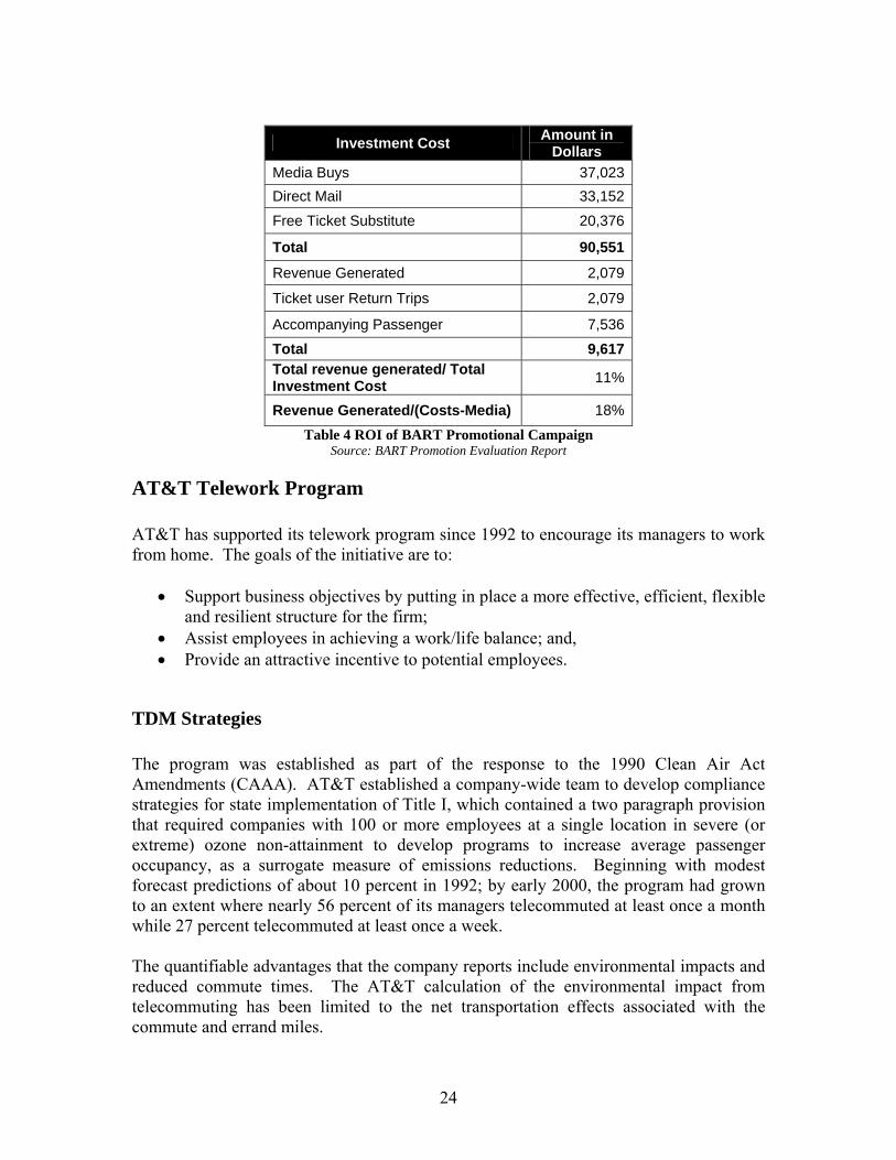
Investment Cost Amount in

Dollars Media Buys 37,023Direct Mail 33,152

Free Ticket Substitute 20,376

Total 90,551

Revenue Generated 2,079

Ticket user Return Trips 2,079

Accompanying Passenger 7,536

Total 9,617Total revenue generated/ Total Investment Cost 11%

Revenue Generated/(Costs-Media) 18%

Table 4 ROI of BART Promotional Campaign Source: BART Promotion Evaluation Report

AT&T Telework Program AT&T has supported its telework program since 1992 to encourage its managers to work from home. The goals of the initiative are to:

• Support business objectives by putting in place a more effective, efficient, flexible and resilient structure for the firm;

• Assist employees in achieving a work/life balance; and, • Provide an attractive incentive to potential employees.

TDM Strategies The program was established as part of the response to the 1990 Clean Air Act Amendments (CAAA). AT&T established a company-wide team to develop compliance strategies for state implementation of Title I, which contained a two paragraph provision that required companies with 100 or more employees at a single location in severe (or extreme) ozone non-attainment to develop programs to increase average passenger occupancy, as a surrogate measure of emissions reductions. Beginning with modest forecast predictions of about 10 percent in 1992; by early 2000, the program had grown to an extent where nearly 56 percent of its managers telecommuted at least once a month while 27 percent telecommuted at least once a week. The quantifiable advantages that the company reports include environmental impacts and reduced commute times. The AT&T calculation of the environmental impact from telecommuting has been limited to the net transportation effects associated with the commute and errand miles.

24

Program Evaluation The AT&T Telework Program evaluation is conducted on an emission reduction basis. Other quantifiable advantages that the company reports include environmental impacts and reduced commute times. Calculation of the environmental impact from telecommuting has been limited to the net transportation effects associated with the commute and errand miles. The AT&T survey studies the average commute lengths for the employees who telework along with the average length of commute. Emission factors used are obtained from the National Environmental Policy Institute (NEPI) and are based on a mass per mile basis, assuming average gasoline mileage. These are multiplied by the estimated savings in commute travel (in miles) to estimate the total savings. These savings were calculated based on the average distribution of days worked at home, the average roundtrip commute distance and net errand miles, and then aggregated to the 67,900 employees reported by AT&T to have teleworked at the time of the October 2000 survey. The total number of miles avoided was 110,000, with 5.1 million gallons of gasoline saved. It must be acknowledged that the impacts rely on the assumption that all telecommuting behavior is assumed to be attributable to the program. It is not clear if any attempt was made to estimate telecommute trends in the region or at other companies over the same period without a similar program. The fact-sheet of the AT&T annual survey of its employees on telework indicates that in 2000, AT&T's employee telework program resulted in:

• Avoidance of 110 million miles of driving to the office; • 5.1 million gallons of gas saved; • Reduction of 50,000 tons of carbon dioxide emissions; • 56 percent of participants teleworking at least one day per month; and, • 27 percent of participants working from home once or more per week.

A key element of the reported programs success has been AT&T’s web portal to promote and educate employees about the Telework Initiative. The web portal simplifies the requirements to set-up a teleworking location by including guidance on how to acquire a computer; how to obtain proper telephone line installation; security issues and formal policies and agreements required.

Evaluating Behavior Change in Transport: Benefit Cost Analysis of Individualized Marketing for the City of South Perth Viewed as a pilot project, this study was carried out in Perth, Australia to encourage a study group to switch to transit, walking and cycling. A benefit cost analysis was developed as part of the assessment process to attract capital works funding for a “no-

25

build” solution to increase use of existing public transport, cycling and walking assets and to defer the demand for future road assets. The funding submission process was successful with $1.2 million dollars being allocated to the project.

TDM Strategies The study was motivated by the premise that travel behavioral change can be brought about by educating individuals separately about the costs and benefits associated with each mode. This strategy, termed individualized marketing, comprises motivational methods to alter travel behavior that reduces one of the major presumed constraints associated with similar promotional efforts: the effectiveness of learning declines over time unless the message is continually reinforced.

Program Evaluation Benefits, costs and transfers are all quantified in three different contexts- socio-economic, public sector finance and private user. Based on the applicability of monetary values, especially for social and environmental impacts, and the derivation and application of implicit or explicit weighting schemes for various components, the costs and benefits can be incorporated into a single evaluation framework. There are two costs associated with this program: setting up the individualized marketing and its continued support, and the cost of improving transit facilities. The benefits are quantified and classified into the following categories:

• Travel Time and Transportation Related Benefits to the User – These include benefits from switching to public transit, cycling costs, walking costs, public transit fares, and the effect of reduced/increased travel times. Travel time costs are estimated based on certain standardized procedures, but the value that is attributed to travel time might vary from person to person and depend on the kind of employment. Different values attributed to travel time make the overall benefit cost ratio different. A value of zero is taken as the base case and then different values are attributed to the travel time and the benefits in each case are quantified.

• User Exposure to Air Pollutants – There may be an aversion to cycling and

walking in heavy traffic owing to vehicle emissions. Research established that car-occupants absorb much higher levels of exhaust pollution than cyclists, walkers or bus passengers (ETA, 1997) [27]. In this exercise, it is stated that this information is likely to have reinforced the substitution for more distant destinations for some trips. Changes in user exposure to air pollution have not been quantified or valued in this evaluation, but it is important to acknowledge that such changes represent a negative impact for those who now choose to walk, cycle or catch public transport (Most reports give numerical values to the air

26

emission levels making them quantifiable also. Hence, benefits are in terms of reduced emission levels and lower pollutant levels).

• Road Trauma – The report states that the road trauma impacts of changes in

travel behavior have two principal components: i. A reduction in road trauma involving motor vehicles; and,

ii. An increase in road trauma involving cyclists and walkers. • Health and Fitness – Substituting more active modes of transport (such as

cycling and walking) for car driving improves the health and fitness of people who make that change. This has been well documented and estimates can be made of the magnitude of some of the impacts, but not generally within a framework suitable for adoption in socio-economic evaluation. There has, however, been useful quantification of increased life expectancy due to cycling activity. Hillman (1997) has estimated that, in the United Kingdom, for every life year lost as a result of increased cycling (bearing in mind that cycling has a higher accident rate than motorized modes), 20 life years are gained through improved health and fitness. Assuming that the same relativity is appropriate in Australia, the 20:1 ratio can be applied to the fatality component (4%) of the road trauma resulting from increased cycle use.

• Congestion Costs – This is an important part of the evaluation procedure. There

are different conditions associated with congestion: i. Marginal cost always exceeds average cost; the cost imposed by one

more car exceeds the cost experienced by each car already on the road; ii. Marginal cost increases with traffic volume - each extra car imposes

successively higher costs; and, iii. Most congestion costs (66% in Melbourne), across the whole road

network imposed by the marginal vehicle are imposed on other road users.

Evaluations are carried out for socio-economic, financial evaluation for public agencies and are carried over horizons of 10 and 30 years. Even on the most conservative assumption in the central evaluation, an investment of $1.3 million in individualized marketing in South Perth would produce benefits of $16.8 million (present value) over 10 years, with a benefit-cost ratio of nearly 13:1. ; including the anticipated benefits through mortality reduction increases the BCR (Benefit Cost Ratio) to 15:1. The report concludes that individualized marketing has been demonstrated to be an effective technique, in South Perth, for changing travel behavior and can deliver benefits that substantially exceed the direct and indirect costs. Using a methodology and values consistent with the evaluation of road projects, the socioeconomic benefits of individualized marketing for South Perth exceeded the costs by a factor of between 11:1 and 13:1, over 10 years, and 12.5:1 to 15:1 over 30 years. These benefit-cost ratios are much higher than those of investments in metropolitan road infrastructure. However, for small increments of travel time, the maximum possible value consistent with the results

27

of the pilot project, the estimate of overall socio-economic return becomes negative in the worst case scenario.

Trip Reduction Performance Program, Washington State Although not related to a specific TDM program or strategy, this case study was deemed as relevant to this research effort. In particular, because it offers an innovative approach to assess the value of TDM by introducing the market based concept where buyers and sellers compete to determine the price of a removed SOV trip. The Commute Trip Reduction (CTR) Performance Grant Program is a pioneer effort in testing whether the Washington State Department of Transportation (WSDOT) can free transportation capacity by removing SOV trips from the existing network infrastructure by means of creating a single buyer market for avoided trips. Established in 2003, the program awards grants on a competitive basis to private employers, public agencies, nonprofit organizations, developers, and property managers who offer financial incentives to their employees and tenants that reduce the number of SOV commute trips taken by their employees and tenants. In 2003, the Washington State Legislature created a framework for the Performance Grant program and engaged the CTR Task Force in obtaining the details in administrative rules. Through the program, WSDOT is trying to create a market for purchasing SOV trips from willing sellers, such as private sector entrepreneurs, non-profit seeking and public sector entities. The program’s objectives are to:

• Purchase avoided SOV trips from willing sellers; • Attract entrepreneurs to trip reduction by offering profit opportunities; and, • Encourage development of innovative trip reduction strategies.

Based on the recommendations of the 1991 CTR Act, which called for the creation of a trip reduction market, the legislature enacted a task force to introduce a performance-based grant program to fund projects that offer financial incentives to commuters to switch from SOV travel. The CTR work force assumed that this would create opportunity for entrepreneurs to invest in trip reduction and create private sector interest in removing trips where additional roadway infrastructure is prohibitively expensive. The 2001 CTR Legislative Report recommended the State Legislature create a trip reduction program to allow WSDOT to purchase removed trips from private parties and attract entrepreneurs to trip reduction by offering profit opportunities. The performance grant program consists of a dual structure; it combines the characteristics of a typical grant program, which awards grants to organizations that submit proposals; and a market program, which buys performance and pays the participants for the number of trip reduced. The legislature and the administrative rules both emphasize that the program is a “grant program” and the performance requirement

28

points to it as a market program, while the award of start-up costs indicates that WSDOT funds projects as well as buys trips. A study was conducted to determine the feasibility of a trip reduction market[28]. Among the findings, two possible markets were identified:

1. A single-buyer market, where the buyer decides the number or trips to be purchased and the price with the presence of multiple sellers; and,

2. A private trading market, with multiple buyers and sellers where the market prices are determined by the law of supply and demand.

The study reported the single-buyer market as the optimal structure, given WSDOT objectives and its public entity status. In this context WSDOT values reduced trips as a good that provides additional roadway capacity and where sellers are entities providing SOV trip reduction strategies measurable in terms of reduced SOV trips. WSDOT would act as a single-buyer on the market. On the other hand, a private trading market is deemed unfeasible due to political and legal hurdles in setting a cap on commute trips, the uncertainty in determining whether the private trading would provide the desired congestion relief, and the ambiguity whether the emission trading markets are a positive strategy in managing air pollution. In this framework, the value of an avoided trip is related to many factors like available funding and underlying price caps. Some of the trip pricing models suggested were:

• Setting a trip value based on the toll amount drivers would pay to drive under reduced congestion, where price would be influenced by factors such as time of day, commute distance, and geographic location;

• Setting a trip value based on the additional infrastructure investment required to add network capacity, which depends on the number of peak users in the corridor; and,

• Establishing a trip value according to available funding and minimum required number of avoided trips.

Ultimately, WSDOT settled for a single-buyer market structure characterized by price caps, with a single statewide cap set at a maximum of $460 per avoided trip. The cap is based on the optimal tolling for the new highway system in the Puget Sound region. In this single-buyer market private employers, public agencies, nonprofit organizations and other entities are invited to compete in selling reduced SOV trips by proposing trip reduction strategies or programs. Each strategy must provide an accurate assessment of its trip reduction efficacy by measuring projected SOV trip reduction against a baseline. This baseline must be measured by means of surveys that report vehicle trips and VMT made by program or project participants. In addition, project performance surveys must be conducted to measure projected vs. actual trip reduction. The requirement of accuracy is defined as “reasonable estimate of employee participation, trip reduction, and VMT reduction,” with no specific guidelines or

29

provisions on estimation methods[29]. Under this framework, in 2006 WSDOT approved 17 projects for the biennium 2005-2007 worth $1.3 million to purchase 3,831 SOV daily commute trips from the state highway system.

30

Proposed Prediction Model In this section, we propose an alternative approach to estimating the impact of TDM strategies. The evaluation framework follows a basic structure for consistent assessment and comparison as found while reviewing relevant guidelines and procedure manuals[11, 12, 18, 19]. The approach embraces the best elements of currently available predictive evaluation methods, while overcoming their constraints identified in the previous section, namely:

• It uses best derived measures of price sensitivity; • It follows a consumer surplus framework; • It captures important transportation users’ trade-offs; • It can assess short and long run impacts; and, • It goes beyond emission control impact evaluation.

Figure 2 outlines the analytical process, which consists of the following steps:

1- Modeling Technique – This step identifies the theoretical framework to predict how a policy change or program implementation will affect travel behavior. The modeling technique overcomes the constraints linked to the use of coefficients derived from generalized travel demand forecasting models, as described in the previous section.

2- Impact Measures – This step links the change in travel behavior to a set of impact measures to be used for evaluation. Impacts are determined in terms of objectives. The objective of this study is to evaluate the impact of TDM in terms of costs and benefits as viewed by a public transportation agency. Therefore, in line with the literature review findings, the impact measures comprise the set of costs and benefits as perceived from a societal viewpoint.

3- Evaluation Metric – In this final step, the impact measures are used within an evaluation approach to determine program effectiveness. The evaluation follows established guidelines that fall within a benefit/cost analysis framework that ultimately prices out the value of a single vehicle trip diverted from the network.

31

Mod

ellin

g Te

chni

que

Eva

luat

ion

Met

ricIm

pact

Mea

sure

sBaseline trips and mode

shares

Change in trips for generalized cost and travel

time policies

Adjust change in tripsfor “soft programs “

Compute final change in Trips, VMT, Mode Shares

Constant elasticity demand model

Relational factors adjustment

Reduced Trip Value

Compute impacts

Program Information

Figure 2 Model Flowchart

32

Modeling Technique In this step, a theoretical model to predict how a policy change or program affects travel behavior in terms of trip change behavior is first identified. The objective is to develop a framework of analysis that can predict the effects on travel decision of diverse and often concurrent TDM strategies. The model predicts changes in the number of mode trips brought about by specific programs or policies. The approach follows the principles governing the law of demand for market goods and is based on price elasticities. Economists have long used the concept of elasticity to describe how individuals react to price changes. The law of demand shows that, in the aggregate, as the price of a good increases its demand declines. This also applies to the demand for transportation goods and services, where prices can take many forms, monetary, such as the cost of using a given mode, and non monetary, such as the perceived cost of time. For example, changes in the cost of travel can affect the number of trips undertaken, the choice of travel time and the choice of mode. The elasticity of demand measures how changes in the price of a good will lead to changes in the quantity purchased and consumption of that good. The elasticity records how the quantity demanded changes in response to a percentage change in its price (and also in the price of competing or complementary goods)[27]. As detailed in this section, the proposed framework allows capturing a broader range of trade-offs that users constantly face and is capable of quantifying impacts on travel patterns by using prices as the direct drivers of travel demand. Furthermore, the approach is able to take into account how individuals re-adjust over time in their trade-offs.

Constant Elasticity Demand for Trips The following example is designed to provide a better understanding of the relationship between price and travel time elasticities and how these relate to travel behavior. Two basic assumptions, which will be relaxed once the model is fully developed and applied in the next section of the report, are made, namely:8

• There are two modes, auto and transit; and, • The major cost drivers are represented by fuel cost and travel times.

Let us assume the following travel demand function:

Tji

Ti

Pi

jiii TTAPd ,εεε= (1) Where: 8 During the spreadsheet design phase, described in the next section of the report, the model is expanded to include more than two modes, additional modal cost drivers, such as transit fare, waiting time, parking costs, and other variable vehicle operating costs.

33

=id demand for auto travel (say vehicle trips per day) j = transit mode A = scale parameter

iP = car travel fuel price

iT = car travel time

jT = transit travel time P

iε = car fuel demand elasticity T

iε = car travel time demand elasticity T

ji ,ε = car travel time cross-elasticity with respect to transit travel time This specific form of the demand function, a constant-elasticity demand function, is chosen because of its wide empirical application in the estimation of travel demand elasticities and for its ease of analytical tractability.9

The fuel price elasticity of a car measures the percent reduction in car vehicle trips due to a one percent increase in its price. The travel time elasticity of demand measures the percent reduction in car vehicle trips due to a one percent increase in travel time. Finally, the car travel time cross elasticity with respect to transit travel time measures the percent reduction in vehicle trips due to a one percent decrease in transit travel time. This assumes that car and transit are substitutes.10 Now, for initial values of fuel price, time and trips, denoted by subscript zeros, the equation will be:

Tji

Ti

Pi

jiii TTAPd ,0000εεε= (2)

9 The demand curves usually employed and depicted in graphs are linear demand curves, which have the property that price elasticity declines as we move down the demand curve. Not all demand curves have this property, however; on the contrary, there are demand curves for which price elasticity can remain constant or even rise with movements down the demand curve. The constant elasticity demand curve is the name given to a demand curve for which elasticity does not vary with price and quantity. Whereas the linear demand curve has the general form: bQaP −= , the constant elasticity demand curve is instead written as:

η1

Q

kP =

Where k and η are positive numbers that determined the shape of the curve. 10 Two goods are considered substitutes if the increase in the price of one determines an increase in the demand for the other. Two goods are considered complements if the increase in the price of one good causes a decrease in the demand for both goods (e.g., coffee and cream). The relationship is further refined by considering perfect versus less-than-perfect substitution and complement.

34

Solving for A in (2) and substituting the results back into (1), we can eliminate the scale parameter and ensure that the demand function passes through the point (d0,P0, T0). The resulting equation is:

Tji

Ti

Pi

j

j

i

iiii T

TTT

PPdd

,

0000

εεε

⎟⎟⎠

⎞⎜⎜⎝

⎛⎟⎟⎠

⎞⎜⎜⎝

⎛⎟⎟⎠

⎞⎜⎜⎝

⎛= (3)

Then, if a policy or program changes the transportation costs and travel times, the new number of vehicle trips is obtained by substituting the new costs and travel times into equation (3), giving:

Tji

Ti

Pi

j

j

i

i

i

iii T

TTT

PPdd

,

0

1

0

1

0

10

εεε

⎟⎟⎠

⎞⎜⎜⎝

⎛⎟⎟⎠

⎞⎜⎜⎝

⎛⎟⎟⎠

⎞⎜⎜⎝

⎛= (4)

Finally, what we are interested in is the change in the number of vehicle trips, which is given by:

⎥⎥

⎦

⎤

⎢⎢

⎣

⎡−⎟

⎟⎠

⎞⎜⎜⎝

⎛⎟⎟⎠

⎞⎜⎜⎝

⎛⎟⎟⎠

⎞⎜⎜⎝

⎛=−=Δ 1

,

0

1

0

1

0

1001

Tji

Ti

Pi

j

j

i

i

i

iiiii T

TTT

PPdddd

εεε

(5)

This last formula constitutes the approach to model the change in demand brought about by program or policies affecting the perceived cost of travel, both monetary and non monetary. Equation (5) can be simplified or expanded to include additional cost factors and to comprise cross relationships with one or more modes as shown in the next section of the report.

Advantages and Constraints The previous section of this report observed that there exist different ways of providing a simple, yet powerful and robust approach to estimating the impacts of alternative strategies at a sketch planning level. For example, the EPA COMMUTER model employs a pivot point approach which relies on the theoretical underpinnings of discrete choice governing travel demand estimation. The EPA choice relies on an individual decision making process among mutually exclusive alternatives, namely different and opposing transportation modes. This is what is usually assumed by all predictive evaluation methods currently available for TDM assessment. The approach proposed herein is capable of estimating mode share changes. It can predict mode share changes not only from SOV to other alternatives, but among these alternatives themselves. It

35

acknowledges substitution and complements effects that might exist between various modes. The constant elasticity of demand approach proposed requires basic information on the cost and time components of modal trips, on the initial mode share. By entering the impact on the generalized cost of travel of a given policy or program, the model estimates the impact on the final mode shares. These data requirements are described in greater detail in the next section of this report. The model estimates impacts on travel behavior in a synergistic fashion. That is, the model allows the simultaneous impact assessment of several TDM policies or strategies, where the final total impacts are greater than the sum of the impact of each individual strategy. In addition, the constant elasticity of demand equation (5) assures that impacts are assessed in a multiplicative, rather than an additive, fashion avoiding impacts overestimation. For example, if one strategy (e.g., a transit subsidy) reduces SOV use by 5 percent and another strategy, say parking pricing, reduces SOV use by an additional 7 percent, the total combined effect is a 11.5 percent reduction( calculated as 100% - [95% x 93%]), rather than a 12 percent reduction (linearly calculated as 7% + 5%). Another advantage of the model is that it allows program evaluation based on incremental impacts. For example, under the constant elasticity demand framework the congestion reduction benefits of a shift from SOV to transit is the difference in congestion impacts between SOV and transit travel. Using a base case approach (a scenario where a policy or program is not implemented), the model estimates the net benefits of shifting from SOV to alternative modes. Also, the model permits distinguishing between peak and off-peak impact estimation at an urban area level. One of the constraints related to the use of elasticities relates to timeframes employed when empirically estimating their values. Applied work generally employs short and medium terms (3-5 years), thus tending to underestimate the full, long term effects of price and service changes. In other terms, increasing (reducing) a transit fare has more negative (positive) effects than what generally predicted by most models.

Soft Program Trip Change Adjustments The preceding model estimates the impact on trip behavior of policies affecting the generalized cost of driving, thus allowing the impact of the following TDM strategies to be captured. The constant elasticity of demand model is best suited for strategies that directly affect the generalized cost of driving, and a set of TDM strategies, such as:

• Parking pricing; • Modal subsidies; • Pay as you go schemes;

36

• Transit service improvements; and, • Other interventions affecting the cost of driving or modal access and travel time.

These strategies often integrate both incentives and disincentives. The latter are usually defined as “sticks” and comprise actions geared at directly influencing the cost of driving, such as increased auto user charges, parking pricing, and traffic calming. All other strategies that are designed to enhance voluntary behavior changes are defined as “carrots” and usually consist of measures geared either at increasing the knowledge of alternative modes and programs or at internalizing some of the costs associated to driving that would otherwise be borne by others. Examples of soft program initiatives include:

• Travel Planning; • Personalized Marketing; • Flexible Work Hours; • Telecommuting; • Guaranteed Ride Home Programs; and, • Discount for Walking and/or Cycling Gear.

Although these programs do not directly affect the cost of using a mode, they tend to impact travel behavior when part of a program consists of hard measures. Generally, it is not possible to directly estimate a prior change in travel behavior of these TDM strategies. The literature review uncovered that the general trend to evaluation is one that relies on culling information from a variety of reports and evaluation analyses to produce a table of diversion rates to then be used to estimate trip change behavior. This approach is followed by the New Zealand Travel Behavior Change Guidance and by the U.K. Department of Transportation Smarter Choice Program. In this report, the approach to evaluate the impact of soft programs on travel behavior relies on an econometric analysis of the relationship between hard and soft programs. Starting with the assumption that voluntary travel behavior initiatives lead to change only in the presence of hard programs, the impact of the following “carrot” initiatives is considered:

• Program Promotion; • Flexible Work Hours; • Telecommuting; • Guaranteed Ride Home Programs; and, • Presence of Amenities (restaurants, ATMs, childcare).

The impact analysis is conducted by building a regression equation where each of these programs enters into an empirical equation estimating the change in ridership as an

37

explanatory variable in a context of interaction with hard programs.11 The regression equation takes the form:

εββββ +++++= kk xxxy ...22110 (7) Where: y = is dependent variable, in this case vehicle trip rate at worksite

kxxx ,...,, 21 = explanatory variables (soft and hard program policies, firm characteristics, other controls)

ε = stochastic or error term Equation (7) can include higher order term to acknowledge nonlinear relationships, and interaction terms between the response variables. Given that the objective is to build a model that can predict the effect on vehicle trip rate reduction of one or more soft program initiatives, worksite trip reduction data between consecutive years are needed. In the analysis, the Washington Sate Department of Transportation Trip Reduction Program dataset was obtained for the period 1995 to 2005. The data reports information on worksite characteristics, such as firm size and industry type, employee mode share, and information of TDM programs. The data were analyzed and factor analysis was employed to reduce the number of explanatory variables to improve model prediction power.12 During the model building phase, several variations of Equation (7) were considered. At the end, a predictive model that allows for interaction between qualitative variables was chosen as the one with the higher predictive power.13 A table of diversion rates was developed based on this predictive model to be used within the sketch planning tool described in the next section of this report14.

11 The model herein proposed to build upon previous work conducted by CUTR in estimating worksite trip reduction tables [30]. 12 Factor analysis is a statistical technique that reduces several variables that are correlated into a smaller set of new, uncorrelated and meaningful variables. 13 In a regression model, qualitative variables take the form of dummy variables. These are explanatory variables that take the value of 1 if present or take the value 0 if absent. For example, dummy variables can be used to estimate main effects due to the presence or the absence of a given program promotion initiative, a given subsidy, and the offering or not of a guaranteed ride home program. Furthermore, very often these initiatives are linked to each other in an interactive fashion. An interaction model has to be built to analyze a main effect model. 14 The diversion rates accompany the model CD.

38

Evaluation Criteria It has been demonstrated how the modeling technique provides a consistent approach to predict travel behavior change brought about by both hard and soft TDM programs. The next step is to link behavioral change to impacts within an evaluation framework that provides cost effectiveness benchmarking and allows TDM to be compared to traditional infrastructure investments. The estimated number of trips reduced must be linked to a set of benefits or impacts. It is therefore relevant to determine what should constitute the set of appropriate benefits to be used for final evaluation. The literature review uncovered two main factors that lead to a proper evaluation of TDM strategies:

• TDM evaluation must be comprehensive, embracing benefits that directly relate to the users and indirectly to all other individuals, and it should

• Lead to a framework of consumer demand conducive to a benefit cost analysis approach for comparative assessment.

The literature on TDM benefits shows how these are directly related to cost generated by SOV use. Generally, costs that are borne directly by the users are defined as internal costs and those costs that are not directly borne by the users are defined as external costs. The latter societal costs belong to what economists describe as negative externalities. Negative externalities arise whenever costs associated with SOV use, such as added congestion delay, air pollution, and increased accident risk, are not directly sustained by auto users but are rather imposed on the society as a whole. Although a comprehensive approach should capture all impacts whether internal or external, the proper set of impacts should be defined based on the nature of the decision-maker. If the evaluation has an employer focus, then the set of impacts might include benefits mainly representing actual savings to employers. If the evaluation is carried out by a public decision making agent, such as a transit agency or a government body, then the set of impacts should be more inclusive of negative externalities. If the evaluation has an employer focus, then the set of impacts might include benefits mainly representing actual savings to employers. Table 5 shows the range of transportation costs categories or TDM benefits that comprise the set of evaluation criteria to be used within the proposed modeling framework. It consists of a subset of all possible impacts that might be generated by TDM policies, focusing on those that can be readily monetized in a consistent and robust fashion. The list of impacts is also consistent with what is currently employed in evaluating traditional infrastructure investments.15

15 Although, in most transportation infrastructure investment decisions a subset of impacts is usually considered, such as travel time, vehicle operating, accident, and pollution costs.

39

Costs Description Type

Vehicle Ownership Vehicle purchase, insurance and other charges Internal-Fixed

Vehicle Operation Maintenance and repair costs Internal-Variable

Travel Time Value of travel time based on prevailing wage rate Internal-Variable

Internal Crash Direct user property damage, personal injury, death Internal-Variable

External Crash Property damage, personal injury, death imposed on others External

Internal Parking Average car parking cost Internal-Fixed

External Parking Land use, capital costs External

Congestion Incremental travel time delay and increased fuel consumption External

Air Pollution Cost of major pollutants: Hydro Carbons (HC), Carbon Monoxide (CO) and Nitrous Oxides (NOx).

External

Other Pollution Includes noise, water and waste (vehicle parts disposal) External

Land Use opportunity cost land devoted to roads External

Other ExternalitiesIncludes costs related to barrier effects, equity, diversity, and other resource externalities

External

Table 5 SOV Cost Externalities

As it will be seen in the next section dealing with the model application, this set of externalities can be expanded or contracted within the sketch planning tool. This grants flexibility to the users by allowing the inclusion or exclusion of given externalities, depending on the program being evaluated or the objectives to be reached.

Evaluation Method: Per Passenger-Trip Average Annualized Benefits In this final step, the impact measures are used within an evaluation approach to determine program effectiveness. The evaluation follows established guidelines that fall within a benefit/cost analysis framework that ultimately prices out the value of a single-vehicle trip diverted from the network. Given that the objective of most (if not all) TDM

40

strategies is to reduce the need for additional SOV trips, the choice of passenger-trip as a unit of measurement allows the most accurate benchmarking measure. The value of a trip removed is measured in annualized dollars per additional passenger-trip. The value of a trip removed is obtained using the following formula: Value of trip removed = Sum (per passenger-trip annualized benefits minus per passenger-trip annualized costs) The unit of measure is expressed in current dollars, and the following procedure shows how to estimate the value of a trip removed and measure it in annualized dollars on a per passenger-trip basis. Equation (5) estimates the number of passenger-trips reduced per day. By assuming that this reduction will last for the duration of the program, the following identity can be established:

= =Trips Reduced/Day

Average Annual Daily Trips (AADT)

Reduced

Average Trips Reduced per Day/Year

The identity signifies that the number of daily passenger-trips reduced stays constant throughout the duration of the program (no additional new daily passenger-trip reduction will be gained during each remaining day of the year). Therefore, the number of daily passenger-trips reduced is equivalent to the average annual daily trips reduced. Next, the daily benefits of the program are computed. This is done by multiplying the number of reduced passenger-trips by the per trip benefit:

X =Trips

Reduced/Day Benefit($)/ Trip Benefit ($)/Day

Next, daily benefits must be annualized. Assuming there are 235 working days in a year,16 then the total annual benefits are computed as:

X = Work Days/Year Benefit ($)/Day Benefit ($)/ Year

Now, recall that the number of daily passenger-trips removed is the same as the average annual daily trips removed, on an annualized basis, the annualized benefits per passenger-trip removed are computed as:

16 This assumes 10 days of holidays, 10 days of vacation, and 5 days of sick leave.

41

/ =Benefit ($)/ Year Annualized Benefits per AADT Reduced

Average Annual Daily Trips (AADT)

Reduced

Next, the formula to convert program costs into an annualized basis is:

( )( ) ⎥

⎦

⎤⎢⎣

⎡

−++

=11

1n

n

iiiPA (6)

Where: A = Annualized value, measured in dollars P = present value, measured in dollars i = annual interest rate n = length of the program, measured in years Another benchmark measure that the model provides is a per passenger-trip benefit to cost ratio, defined as the ratio of annualized per passenger-trip benefits to per passenger-trip costs:

/ =Annualized Benefits/ AADT Reduced

Annualized Costs/ AADT Reduced Benefit/Cost Ratio

As seen in the following example, this last measure provides a metric suitable for intra-comparison across different competing TDM alternatives and for inter-comparison, i.e., TDM strategy versus capacity expansion.

Applied Example: Transit Travel Time Improvement and Parking Cost Increase A simple example provides some insight on how the constant elasticity of the demand model can be used to estimate impacts on travel behavior produced by changes in the generalized costs of two modes. We start by defining a base case scenario (absence of program strategy) by assuming a set of initial cost and travel time values for both SOV and transit:17

• 3,000 vehicle round trips per day =id• = $6.00 current daily SOV parking cost 0iP

17 Elasticity estimates are obtained from Litman [28]. The study provides a summary of various elasticity estimates culled from several publications.

42

• = 15 minutes two way auto travel time 0iT

• = 15 minutes two way auto travel time 1iT

• = 30 minutes two way transit travel time 0jT

• =-0.08 parking price elasticity Piε

• = -0.225 auto travel time elasticity Tiε

• = 0.036 auto travel cross time elasticity with respect to transit Tji ,ε

• = Auto i• j = Transit

Next we introduce a trip reduction strategy that reduces transit travel time by 10 minutes and increases SOV parking cost from $6.00 to $9.00 per day. The program details and costs are as follows:

• = $9.00 new daily SOV parking cost 1iP

• = 20 minutes new two way transit travel time 1jT• $50,000 program implementation cost • n = 2 program length (years) • i = 6.00% current interest rate[30]

With these initial base case scenario values, the demand for SOV trips is equal to 3,000 round trips per day. Next, we use Equation (5) to estimate the change in vehicle trips brought about by a transit improvement that reduces the overall travel time by 10 minutes, and an increase in car parking costs from $6.00 to $9.00 daily. Following this approach, it suffices to plug in the above values in Equation (5) to obtain the change in vehicle trips per day as a result of the combined effect of transit improvement and car parking policy. The estimation produces a decrease of 138 vehicle trips, or 5 percent, based on the initial elasticity assumptions:18

13812030

1515

00.600.9000,3

036.0225.008.0

−=⎥⎥⎦

⎤

⎢⎢⎣

⎡−⎟

⎠⎞

⎜⎝⎛

⎟⎠⎞

⎜⎝⎛

⎟⎠⎞

⎜⎝⎛=Δ

−−

id

It is relevant to note that the total number of trips reduced is the result of a multiplicative effect of the two policies affecting parking pricing and transit travel time. Each of these policies has a direct and indirect impact on travel demand, as detailed in Figure 3, which displays the demand for SOV trips.19 Let Tj be the travel time of the alternative mode, in

18 Note that trips do not add up for each day that goes by, as to say that the first day we reduce 138 trips and the next day we reduce another 138 new trips. These reduced trips are recurring reduced daily trips and are to be considered as annual daily vehicle trips or ADDT, if we wish to use the acronym normally employed in transportation demand modeling. 19 For ease of display, the demand curve is represented as a linear function, while the constant elasticity is curvilinear in nature. The graph is not to scale.

43

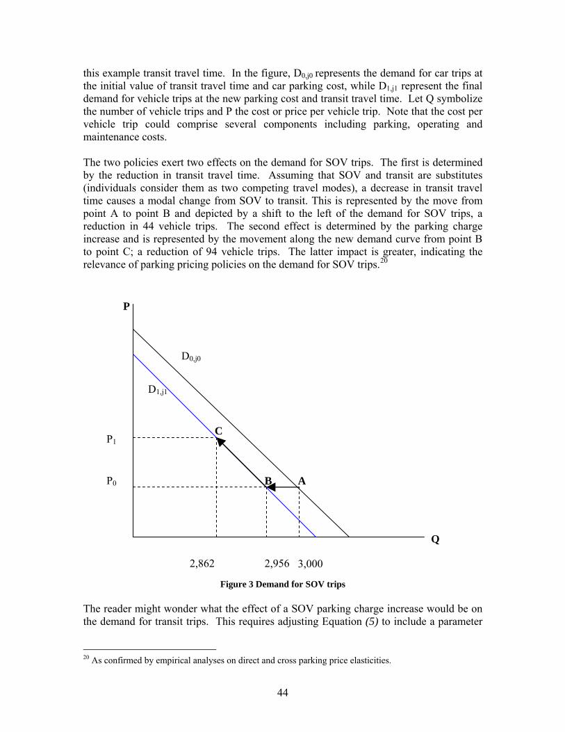
this example transit travel time. In the figure, D0,j0 represents the demand for car trips at the initial value of transit travel time and car parking cost, while D1,j1 represent the final demand for vehicle trips at the new parking cost and transit travel time. Let Q symbolize the number of vehicle trips and P the cost or price per vehicle trip. Note that the cost per vehicle trip could comprise several components including parking, operating and maintenance costs. The two policies exert two effects on the demand for SOV trips. The first is determined by the reduction in transit travel time. Assuming that SOV and transit are substitutes (individuals consider them as two competing travel modes), a decrease in transit travel time causes a modal change from SOV to transit. This is represented by the move from point A to point B and depicted by a shift to the left of the demand for SOV trips, a reduction in 44 vehicle trips. The second effect is determined by the parking charge increase and is represented by the movement along the new demand curve from point B to point C; a reduction of 94 vehicle trips. The latter impact is greater, indicating the relevance of parking pricing policies on the demand for SOV trips.20

P1

P0

D0,j0

D1,j1

3,000 2,956 2,862

A

C

B

P

Q

Figure 3 Demand for SOV trips

The reader might wonder what the effect of a SOV parking charge increase would be on the demand for transit trips. This requires adjusting Equation (5) to include a parameter

20 As confirmed by empirical analyses on direct and cross parking price elasticities.

44

to represent the cross-price elasticity of transit trips with respect to auto parking price. This is done in the full extension of Equation (5) of the sketch planning application. Indeed, this approach can be extended to evaluate all TDM programs or strategies affecting the generalized costs of transport and modal travel times. The estimated change in SOV trips can subsequently be used within a social welfare framework of analysis. For example, the number of SOV diverted trips can be evaluated in a benefit cost analysis fashion, where each reduced trip is valued for the societal benefits it contributes to, and discounted by the cost incurred to divert it to other modes. The next step of the evaluation is to assess the net annualized benefits that these 138 reduced vehicle trips provide. Let us assume that the sum of per passenger-trip external costs associated with SOV is equal to $2.00 per round trip. Therefore, the average daily benefits brought about by the 138 reduced trips are:

(138 trips/day) X ($2.00/trip) = $276/day Assuming an average of 235 working days per year, the annual benefits are equal to:

($276/day) X (235 days/year) = $64,782/year Since the number of daily passenger-trips reduced is equivalent to the average annual daily trips (AADT) reduced, the annualized per passenger-trip benefit is equal to:

($64,782) / (138 AADT reduced) = $470 per AADT reduced

Now, we turn to compute the annualized cost of the program, by plugging the example numbers into Equation (6):

( )( )

272,27$106.01

06.0106.0000,50 2

2

=⎥⎦

⎤⎢⎣

⎡

−++

=A

Which on a per AADT reduced basis is equivalent to:

($27,272)/(138)= $ 198 per AADT reduced

Finally, the value of a trip removed is equal to the sum of benefits and costs: Value of trip removed (per AADT reduced) = $470 - $198 = $272 Another significant measure of the program effectiveness is given by the benefit to cost ratio, which is equivalent to:

$470 / $198 = 2.40

45

The latter means that for every one dollar invested in the TDM policy there is a gain of $2.40 in overall benefits. Both the value of the trip removed and the benefit to cost ratio are measures of effectiveness widely used for program benchmarking and evaluation.

46

Model Implementation: TRIMMS To translate the theoretical framework of the prediction model developed in the previous section, we developed a sketch-planning model in the form of a spreadsheet module. Sketch-planning models represent a class of rather straightforward models that focus on the initial or screening phases of analysis. These models are used for situations where performing a more sophisticated analysis is not possible, or requires a costly effort in terms of data gathering. Spreadsheet modules or applications represent an ideal tool for the first phases of planning and estimation. They are designed in a way which allows someone other than the developer to perform useful work without extensive training. Spreadsheets enable the end user to perform a diverse set of analyses using efficient methods and algorithms to produce accurate results, utilizing an interface that is clear and consistent. Modules can be designed in a fashion so that they can be modified with minimum effort and maximum flexibility; they are portable and run on any system that has commonly used software. The spreadsheet model takes the acronym of TRIMMS, Trip Reduction Impacts of Mobility Management Strategies. The model takes its name from its main characteristic, namely the estimation of the value of a passenger trip removed as a result of a TDM policy. Figure 4 depicts the internal structure of TRIMMS, which follows from the theoretical framework developed in the previous section. Starting from a base case scenario representative of the program or strategy being evaluated, the constant elasticity model estimates final mode share changes, resulting in hard program impacts. If the evaluation extends to soft programs, such as program promotion or any other voluntary behavioral change measure, a separate module is designed to estimate the impacts. The evaluation is carried out in an interactive fashion where the user answers a set of questions, whose results are used to call a priori estimated diversion rates. The final impact shares are then used to conduct the social welfare analysis that leads to the production of the evaluation metric explained in the previous section, namely the value of a trip removed.

47

Baseline Case Scenario

Hard Program Impacts - Financial Incentives - Financial Dis-incentives

Baseline Inputs- Trip Split- Mode Share- Travel Times

Trip Demand Estimation -Constant Elasticity of Demand Model

Soft Program Impacts - Program Promotion - Guaranteed Ride Home - Flexible Work Hours - Telecommuting - Amenities

Hedonic Regression Analysis

Model Output

Change in baseline trips - New - Diverted - Change in final mode shares - Change in final VMT

Social Welfare Analysis- Added & reduced externalities

Benefit Measures- Health and Safety- Congestion- Emission Pollution- Land Use Impacts- Other

Value of Trip Removed

- Net per passenger trip annualized benefits- Net per passenger trip annualized program cost- Peak and off-peak values- Benefit to cost ratio

Figure 4 TRIMMS – Inner Layout

48

Defining the Base Case: Input Requirements To function correctly, the model needs a set of input data that altogether define the base case scenario. The base case defines the status of a program in its current shape and form, without the implementation of the proposed policy or strategy.

• Program Information - This consists of information on the base case scenario, where program characteristics are described.

• Individual Information – This consists of information on the number of users

the policy will affect. Usually this comprises the pool of employees participating as being part of a TDM program.

• Trip Data – This includes information on mode shares, average trip length and

travel time by mode, and average vehicle occupancy. This information is entered into a worksheet tab entitled “Base Case Scenario,” which is displayed in Figure 5.

Figure 5 TRIMMS – Base Case Scenario Worksheet

When entering the program information, the user can select the year the analysis is being conducted and all costs and benefits are immediately adjusted to current dollar values. Next, the user is directed to estimate the impact of several program strategies or policies. Following the literature on TDM strategies, impact evaluation is split into hard program

49

and soft program evaluation. Hard program evaluation is split into two separate worksheets, each allowing the assessment of a wide range of policies or strategies having a direct impact on the generalized cost of travel and the value of time. At the click of a button, the model can be fully customized by modifying all of the default cost and trip demand function parameters, as explained in further details in this section. Financial Incentives and Disincentives In this worksheet, different TDM strategies affecting the cost of travel can be assessed. These include programs or policies geared at penalizing the cost of SOV use (the so called “sticks”), such as;

• SOV parking price changes; • Pay-as-you-go schemes; and, • Other policies affecting the cost of SOV use.

This worksheet also allows estimation of the impact of TDM incentives (“carrots”) directly affecting the cost of driving alternative modes either by directly lowering the cost of using a mode or indirectly in the form of a subsidy. Figure 6 provides a snapshot of the Financial Incentives worksheet.

Figure 6 TRIMMS - Financial Incentive Worksheet

50

Travel Time Improvements In this worksheet the user can evaluate the impact of strategies affecting modal travel time. Figure 7 shows that the model differentiates between access and travel time, thus allowing the user to assess the impact of strategies that affect the two most relevant components of travel time. The model allows the evaluation of a single policy or the simultaneous assessment of a portfolio of strategies representing a mix of “sticks” and “carrots” to understand how policies are interlinked. Sensitivity analysis of the sketch-planning model showed that the final impact of the value of a trip removed is dependent upon the following assumptions:

• Program size and characteristics (employee initial modal split); • Policy being evaluated (single policy vs. a package of incentives and

disincentives); and, • Mix of financial incentives and travel time improvements.

In particular, the value of a trip removed is relatively sensitive to a policy affecting the cost of parking. The impact is relatively greater if additional policies are considered, such as applying a subsidy and a travel time improvement on transit services.

Figure 7 TRIMMS – Travel Time Improvements Worksheet

Soft Program Impacts In this worksheet, the user can evaluate the following initiatives:

51

• Program Promotion; • Flexible Work Hours; • Telecommuting; • Guaranteed Ride Home Programs; and, • Presence of Amenities (restaurants, ATMs, childcare).

As discussed in the previous section, these measures fall into the definition of “carrots” to indicate those policies that are intended to voluntarily promote change in travel behavior. The literature review and case study analysis revealed that there exists an abundance of such policies, whose impact on travel behavior is difficult to estimate. As previously described, while these strategies do not have a direct impact on the cost of driving or the value of travel time, they exert an indirect effect on the choice of alternative modes. Furthermore, their impact on final modal share is the result of the absence or presence of hard program measures. In this worksheet, the user is guided through several steps where he/she is asked to answer several questions as displayed in Figure 8. Based on the answers, final modal shares are provided to evaluate soft program impacts. In the presence of hard program measures, these sets of questions serve to balance the final modal share to provide a combined evaluation of soft and hard program measures. The user is asked to fill information on the following steps:

1. Industry Classification; 2. Worksite Characteristics; 3. Program Marketing; 4. Program Subsidies; 5. Guaranteed Ride Home and Ride Match; and, 6. Telecommuting and Flexible Work Hours.

52

Figure 8 TRIMMS – Step by Step Soft Program Evaluation

The user is guided through a set of questions comprising the six screens. Based on the answers provided, the model automatically applies a set of diversion rates, which were derived using the soft program estimation procedures outlined in the previous section. Just like in the case of hard program evaluation, the user has the option to override the model and manually supply the final mode shares.

Model Output Figure 9 shows the layout of the Model Output worksheet. All policies or strategies being evaluated are summarized and their impact is presented and summarized by employing the evaluation metric of choice discussed in the previous section. The layout is similar to that of the EPA Commuter 2.0, to provide continuity to those practitioners already accustomed to pollution emission evaluation. The user can create custom charts by clicking on command buttons located on the worksheet, as well as go back to the “Base Case Scenario.” To better understand how to read and interpret the results, the next section of the report provides application examples.

53

Figure 9 TRIMMS – Model Output

54

Customizing the Model TRIMMS has been designed to be fully flexible and customizable by the end user. To allow modification of assumption and results, the model permits full customization of the following:

• Modal Cost Externalities; • Travel Demand Function Elasticities; and, • User Supplied Final Modal Shares.

In every step of the analysis, the user can modify these three main factors and is encouraged to customize the model to better fit it to the analysis context. Below, each of these factors is discussed in terms of effects and implication on the model results. Modal Cost Externalities In the “Base Case Scenario” worksheet, the user can click on the “Modify Model Parameters” button. This opens a window that shows a series of tabs, each allowing modification of the externalities cost parameters as displayed in Figure 10. The cost parameters are measured in actual dollars per passenger-trip units and are split in peak and off-peak values. These can be accessed by clicking on the apposite tabs. Note that by setting the values to zero, the user can override the model for including a given externality in the evaluation process. For example, if the user is interested in just evaluating the health and safety impacts of a given program or strategy, he or she can set the remaining externality cost values equal to zero. The model will then run and evaluate results only considering health and safety impacts to estimate the value of a passenger trip removed. Throughout this step by step process, the user is allowed to cancel the operation at any time leaving the model unchanged. A final confirmation is also required to modify the model. Once the model is changed, it can always be reverted to its defaults by clicking on the “Model Reset” button.

55

Figure 10 TRIMMS – Model Parameters Modification

Travel Demand Functions Elasticity Parameters The user can also modify the modal trip demand function elasticity parameters. This allows adapting the trip demand functions to ad-hoc situations where the user possesses better information on how individuals react to price changes or policies affecting access and transit travel time. To modify the elasticity parameter the user must click the “Modify Model Parameters” button and then click on the “Elasticities” tab. This provides access to the window displayed in Figure 11. The user can experiment with the default values by slightly modifying them to see how the model results are sensitive to parameter modification. As in the case of the per passenger-trip cost externalities, the user can close the window and leave the model unchanged. Once the model is modified, it can always be reset by clicking the “Model Reset” button.

56

Figure 11 TRIMMS – Price and Travel Time Elasticity Parameters Modification

User Supplied Final Mode Shares The model’s strength is its capacity to estimate the impact on final mode shares of a given policy or strategy. This is accomplished by means of the constant elasticity of the demand model as described earlier in the report. Whenever the user possesses specific information or a guess estimate about the potential impact a given policy might have on final mode share, he or she can override the model by manually entering the values. This option is accessible from the “Financial Incentives,” “Travel Time Improvements,” and “Soft Program Evaluation” worksheets by clicking on the “Supply Final Mode Shares” button. This opens a window as displayed in Figure 12. The user enters the new mode shares (in percentage points) and then clicks the “Ok” button. A final warning displays to confirm the decision to over ride the model. The model can always be reset by clicking on the “Model Reset” button. If the user supplied shares sum is not equal to 100 percent, a warning message informs the user of this imbalance. Nonetheless, the model automatically rebalances the final mode share to total 100 percent. Note that although the “Model Output” worksheet displays the user supplied final mode shares, the balanced shares are used to compute impacts.

57

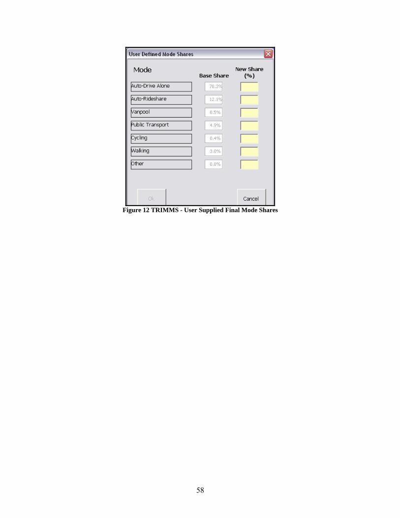
Figure 12 TRIMMS - User Supplied Final Mode Shares

58

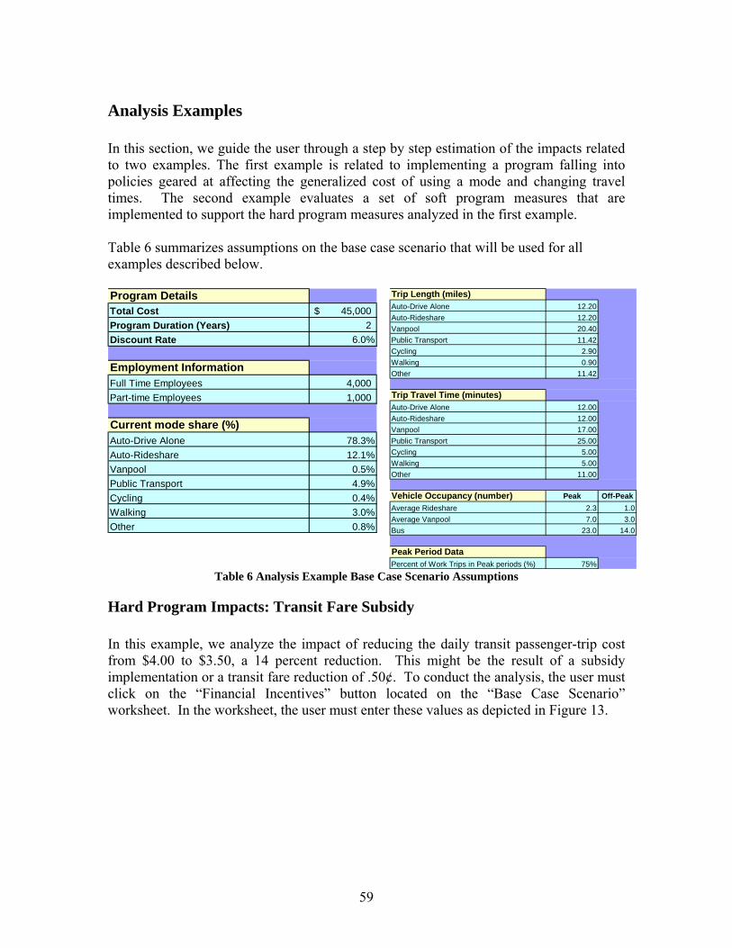
Analysis Examples In this section, we guide the user through a step by step estimation of the impacts related to two examples. The first example is related to implementing a program falling into policies geared at affecting the generalized cost of using a mode and changing travel times. The second example evaluates a set of soft program measures that are implemented to support the hard program measures analyzed in the first example. Table 6 summarizes assumptions on the base case scenario that will be used for all examples described below. Program Details Total Cost 45,000$ Program Duration (Years) 2 Discount Rate 6.0%

Employment InformationFull Time Employees 4,000 Part-time Employees 1,000

Current mode share (%)Auto-Drive Alone 78.3%Auto-Rideshare 12.1%Vanpool 0.5%Public Transport 4.9%Cycling 0.4%Walking 3.0%Other 0.8%

Trip Length (miles)Auto-Drive Alone 12.20Auto-Rideshare 12.20Vanpool 20.40Public Transport 11.42Cycling 2.90Walking 0.90Other 11.42

Trip Travel Time (minutes)Auto-Drive Alone 12.00Auto-Rideshare 12.00Vanpool 17.00Public Transport 25.00Cycling 5.00Walking 5.00Other 11.00

Vehicle Occupancy (number) Peak Off-PeakAverage Rideshare 2.3 1.0Average Vanpool 7.0 3.0Bus 23.0 14.0

Peak Period DataPercent of Work Trips in Peak periods (%) 75%

Table 6 Analysis Example Base Case Scenario Assumptions

Hard Program Impacts: Transit Fare Subsidy In this example, we analyze the impact of reducing the daily transit passenger-trip cost from $4.00 to $3.50, a 14 percent reduction. This might be the result of a subsidy implementation or a transit fare reduction of .50¢. To conduct the analysis, the user must click on the “Financial Incentives” button located on the “Base Case Scenario” worksheet. In the worksheet, the user must enter these values as depicted in Figure 13.

59

Figure 13 TRIMMS – Transit Fare Subsidy

Finally, to view the results, it is sufficient to click the “View Results” button. Figure 14 displays the outcome. The lower fare results in a total reduction of 109 daily vehicle trips, with a net value of a trip removed equal to $645.00, and a benefit cost ratio of 2.8.

Figure 14 TRIMMS - Transit Fare Subsidy Impact

60

Next, in conjunction with the policy just implemented, we consider implementing a $1.00 daily parking surcharge on SOV users that increases average daily parking costs from $6.00 to $7.00. To estimate the final impact, it is sufficient to click on the “Financial Incentives” worksheet and enter the parking cost values as displayed in Figure 15.

Figure 15 TRIMMS – Transit Subsidy and Parking Surcharge

By clicking the “Results” button the new impacts are summarized. Figure 16 shows the result indicating that the combined effect of the two policies leads to a reduction of 178 vehicle trips, a net trip removed value of $821.00 and a benefit to cost ratio of 5.5. The user can also chart the final mode share impacts by clicking the appropriate button on the “Results” worksheet, as displayed in Figure 17. The chart provides some insight about the impact of the transit subsidy and parking surcharge on mode shares. While the transit subsidy has the effect of diverting SOV vehicle trips, the parking surcharge both diverts vehicle trips to transit and all other modes, in a particular rideshare (an increase of 0.2%).

61

Figure 16 TRIMMS – Transit Subsidy and Parking Surcharge Impacts

Mode Share Impacts

-10.0%

0.0%

10.0%

20.0%

30.0%

40.0%

50.0%

60.0%

70.0%

80.0%

90.0%

Baseline 78.3% 12.1% 0.5% 4.9% 0.4% 3.0% 0.8%

Final 77.6% 12.3% 0.5% 5.3% 0.4% 3.1% 0.8%

% Change -0.7% +0.2% +0.0% +0.4% +0.0% +0.1% +0.0%

Auto-Drive Alone Auto-Rideshare Vanpool Public Transport Cycling Walking Other

Figure 17 TRIMMS – Transit Subsidy and Parking Surcharge Final Mode Share Impacts

62

Soft and Hard Program Impacts Next, the additional impacts of a set of initiatives geared at promoting voluntary change in travel behavior are considered. The previous example are expaned to assess the impacts related to program promotion through a set of marketing initiatives and the implementation of telecommuting and flexible working schedules. To conduct the analysis, the user must press the “Soft Program Evaluation” button located in the “Base Case Scenario” worksheet. This opens a separate window consisting of a step-by-step set of tabs asking questions related to soft programs. Based on the answers, specific diversion rates are used to estimate final mode share changes. The user can always override the model by clicking the “Supply Mode Final Mode Shares” button. First, the user must select the appropriate industry sector that the organization being evaluated belongs to. In this example, it is assumed that the organization’s major functions fall under finance, insurance and real estate.

Figure 18 TRIMMS – Soft Program Module: Step One

63

Next, the user is asked a set of questions related to the presence or absence of accessibility enhancements (bus stops, bike lanes, and sidewalks), worksite amenities and parking facilities/arrangements. In this example, it is assumed that the worksite provides bus stops, bike lanes and sidewalks within ¼ mile radius. In addition, ATM, and restaurant facilities are present, as well as the provision of rideshare parking.

Figure 19 TRIMMS – Soft Program Module: Step Two

In step three, the user is asked a question related to program marketing promotion, both inside and outside the organization. Marketing campaigns are essentially divided into two categories: those designed to specifically target individuals within the organization and those conceived to increase awareness and potential participation at a regional area level.

64

Figure 20 TRIMMS – Soft Program Module: Step Three

Next, the user is asked to enter information on the presence of any ongoing subsidy program.

65

Figure 21 TRIMMS – Soft Program Module: Step Four

In step five, there is information on Guaranteed Ride Home (GRH) programs that provide an occasional subsidized ride to commuters who use alternative modes. For example, if a vanpool user must return home in an emergency, or a carpooler must stay at work later than expected, the employer guarantees the ride back home.

66

Figure 22 TRIMMS – Soft Program Module: Step Five

Finally, in step six, the user answers questions related to the implementation of telecommuting and/or flexible working schedules. In step six the user is asked if the organization offers special arrangements that allow individuals usually working a fixed schedule to alter their daily working hours. In this report, the following definitions are employed:

• Alternative Work Schedules (also called Variable Work Hours) include:

o Flextime. In this arrangement employees are allowed some flexibility in their daily fixed work schedules that permits them to get to work earlier or later depending on their situation.

o Compressed Workweek: where employees work fewer but longer days, such

as four 10-hour days each week (4/40), or 9-hour days with one day off every two weeks (9/80).

67

o Staggered Shifts: where work shifts are staggered to reduce the number of employees arriving and leaving a worksite at one time. For example, some shifts may be set to start from 8:00 a.m. to 4:30 p.m., others from 8:30 a.m. to 5:00 p.m., and others from 9:00 a.m. to 5:30 p.m.

• Telecommuting: refers to salaried employees who are allowed to work from home

or another location (such as a telework center) to reduce commute travel.

Figure 23 TRIMMS – Soft Program Module: Step Six

By clicking the “Finish” button, the module closes and the model automatically switches to the “Results” worksheet. The final mode shares previously estimated and displayed in Figure 16 are adjusted to compensate for the impacts produced by the soft program evaluation and are displayed in Figure 24. The combined effect of a soft and hard program produced a reduction of 241 vehicle trips, a net benefit of $871.00 at urban peak values, and a benefit to cost ratio of 8.0.

68

Figure 24 TRIMMS Combined Hard Program/Soft Program Impacts

69

Conclusions The report summarized the approaches used to date, conceptualized a new approach and introduced a model that allows some regions to use local data or opt to use defaults from national research findings, select the benefits and costs of interest, and calculate the costs and benefits of the program. The model, TRIMMS, resulting from this project provides a comparative assessment of TDM for program managers and funding agencies like FDOT to make informed decisions on where to spend finite transportation dollars based on a full range of benefits and costs. The approach is consistent with other benefit/cost analyses. Its accuracy and the perceived fairness are critical when significant funds are at stake. A key strength of this model is its wide range of benefits and costs that can be selected for the analysis. The model’s flexibility and robustness allow it to be adopted by agencies throughout the country. This model focuses on the societal costs and benefits at a regional or worksite level. Future research could seek to enhance the model to include more of the internal benefits to employers (e.g., changes in worker productivity, reduction in overhead, changes in employee retention, etc.). Certainly, the challenge of this future enhancement is finding data relating to given TDM strategies to such business outcomes, given businesses seeking to maintain a competitive advantage. Another area of future research would be to develop regional or local values for some of the externalities and elasticities. Finally, a byproduct of this research effort that goes beyond the initial research objectives is the development of a structured approach to evaluate the impact of soft programs. Compared to the currently available soft program evaluations methods, the approach developed in this report provides a less heuristic method of estimation resulting in statistically robust mode share impact predictions. Another future area of analysis would be the refinement of such a model to provide a standardized approach to soft program impact assessment.

70

References 1. CMAQ, C.M.a.A.Q.I.P., Interim Program Guidances, F.H. Administration,

Editor. 2006, US Department of Transportation. p. 25-26. 2. WSDOT, W.S.C.T.R.P., CTR Task Report to the Legislature. 2005, Washington

State Department of Transportation: Olimpia, WA. p. 61. 3. Schreffler, E., State of the Practice: Mobility Management Monitoring and

Evaluation in the United States in MOST: Mobility Management Strategies for the Next Decades,Work Package 3, D3 Report, Appendix C 2000.

4. Office, A.G., Evaluation of 26 Australian TravelSmart Projects in the ACT, South Australia, Queensland, Victoria, and Western Australia. 2006, Department of Environment and Heritage: Canberra, Australia.

5. Maunsell, P.R.a.B.A.H., Travel Behaviour Change Evaluation Procedures- Literature Review. 2004, Transfund New Zeland/EECA: Melbourne, Australia.

6. Maunsell, P.R.a.B.A.H., Travel Behaviour Change Evaluation Procedures- A Technical Report. 2004, Transfund New Zeland/EECA: Melbourne, Australia.

7. EPA, Procedures Manual for the COMMUTER Model v2.0. 2005, Environmental Protection Agency.

8. EPA, COMMUTER Model v2.0 User Manual. 2005, Environmental Protection Agency.

9. FGM-AMOR – Forschungsgesellschaft Mobilität, A.M.R., MOST Mobility Management Strategies for the Next Decades. 2003, European Community Competitive and Suistainable Growth Programme.

10. CUTR, TDM in Europe: A Synthesis of Research Findings. 2003: CUTR NCTR. 11. VTPI, TDM Evaluation - Assessing Benefits and Costs. 2006, Victoria Transport

Policy Institute. 12. VTPI, Transportation Costs & Benefits Resources for Measuring Transportation

Costs and Benefits, in TDM Encyclopedia, V.T.P. Institute, Editor. 2005, Victoria Transport Policy Institute.

13. Litman, T., Transportation Cost and Benefit Analysis; Techniques, Estimates and Implications, in TDM Encyclopedia, V.T.P. Institute, Editor. 2002.

14. Litman, T., Guide to Calculating TDM Benefits, in TDM Encyclopedia. 1999, Victoria Transport Policy Institute.

15. Phil L. Winters, H.S.J., Quantifying The Business Benefits of TDM. 2003, Center for Urban Transportation Research, for the Office of Research and Special Programs, Florida Department of Transportation.

16. TCRP, TCRP 107 Analyzing the Effectiveness of Commuter Benefits Programs, in TCRP, T.C.R. Program, Editor. 2005, Transportation Research Board.

17. Schreffler, E.N., Alternative Modes as an Air Quality Mitigation Strategy – Final Report 566. 2004, Arizona Department of Transportation

18. VTPI, Comprehensive Transport Planning, in TDM Encyclopedia, V.T.P. Institute, Editor. 2005, Victoria Transport Policy Institute.

71

19. Board, T.R., The Congestion Mitigation Air Quality Improvement Program: Assessing Ten Years of Experience, in Special Report 264. 2002, National Academies.

20. Washington, U.o., U-PASS Annual Report. 2004, University of Washington. 21. Washington, U.o., U-PASS Telephone Survey Report. 2004, University of

Washington. 22. Washington, U.o. U-PASS Fact Sheet. 2001 [cited; Available from:

http://www.washington.edu/upass/news_and_reports/reports.html. 23. Seattle, C.o., Way to Go, Seattle! Program Evaluation Summary Report. 2002,

City of Seattle: Seattle. 24. PSRC, The Cost of Transportation; Expenditures on Surface Transportation in

the Central Puget Sound Region for 1995. 1995, Puget Sound Regional Council. 25. VTPI, Health and Fitness, in TDM Encyclopedia, V.T.P. Institute, Editor. 2002,

Victoria Transport Policy Institute. 26. BART, Hayward "Heavy Up" Promotion Evaluation. 2005, BART Marketing and

Research. 27. Nicholson, W., Microeconomic Theory Basic Principles and Extensions. 7 ed.

1998: Dryden Press. 198-200. 28. Daniel Carlson, J.S., Zack Hill, Alex Atchinson, The CTR Performance Grant

Program: Strengthening the Program's Structure and Market, W.S.T. Commission, Editor. 2005, Washington State Transportation Center: Seattle.

29. WSDOT, Guide to Trip Reduction Program, W.S.D.o. Transportation, Editor. 2005, Washington State Department of Transportation.

30. Office of Management and Budget, E.O.o.t.U.P., Discount Rates for Cost-Effectiveness, Lease Purchase,and Related Analyses - Appendix C. 2007.

72