Economics of Uncertainty:Behavior, Perceptions and Policy-Making

Bergen, NHH, intensive PhD courseApril 11-15, 2011

Nicolas TreichLERNA, Toulouse School of Economics

ntreich@toulouse.inra.frwww.toulouse.inra.fr/lerna/treich/indextreichd.htm

Preliminary Remarks

• This lecture presents– some classical models– as well as some recent behavioral models

• Discuss what our models mean, and imply• Theory-oriented but empirical (and

experimental) aspects won’t be ignored

Organization

• 4 days of class• + last day: presentation of recent papers

by students• Give exercises, and assign a paper (i.e.

home work)• Validation (need half of 5+5+10)

Recommended Books• Eeckhoudt L., C. Gollier and H. Schlesinger, 2005, Economic and Financial

Decisions under Risk, Princeton University Press. • Wakker, P, 2010, Prospect Theory: For Risk and Ambiguity, Cambridge

University Press.

• Gilboa, I., Rational Choice, 2010, MIT Press. • Gollier C., 2001, The Economics of Risk and Time, MIT Press• Hirshleifer J. and J. Riley, 1994, The Analytics of Uncertainty and Information,

Cambridge University Press. • Ingersoll J.E., 1987, Theory of Financial Decision-Making, R & F Editors.• Kagel J. and A. Roth, 1995, The Handbook of Experimental Economics, Princeton

University Press. • Kahneman D., P. Slovic and A. Tversky, 1982, Judgment under Uncertainty:

Heuristics and Biases, Cambridge UP. • Slovic P, 2000, Perception of Risk, Earthscan Publisher. • Thaler R. and C. Sunstein, 2009, Nudge. Improving Decisions about Health, Wealth

and Happyness. Yales University Press. • Viscusi K., 1998, Rational Risk Policy, Princeton University Press.

Outline1. Introduction

2. Basics: Expected Utility and Risk Aversion3. Choice in Risky Situations

4. Experimental Economics5. Non-Expected Utility Models6. Risk Perceptions and Ambiguity

7. Some Policy Implications

1. Introduction

Why is the study of risk important?

All decisions involve the future, and so involve risk

The management of risk is what best explains economicdevelopment (Bernstein 1998)

Biggest sectors in our economies: insurance and finance

Environmental risks (e.g., climate change damages estimates may reach 5% to 20% of GDP, Stern 2007)

Useful for general education in economics (e.g., information economics)

Main Objective of the Field

• Find a model of individual behavior in situations of risk and uncertainty

• Remark: It is usually said that risk (resp. uncertainty) when probability known (resp. probability unknown), but difference will berefined

Which behavior in face of risk?Why not taking the « expected value » after all?

- Any other criterion, if used repeatedly will almost certainlyleave less well off at the end

- But, would you bet $100 on the outcome of the flip of a coin? $100,000?- People buy insurance (transform risk into its expected value and pay a premium for this)- Risk premia on financial markets

- However, people gamble! (casino, PMU…)

Expected ValueWhy not taking the « expected value » after all?

- St Petersburg’s paradox (1713): A fair coin will be tossed until a head appears; if the first headappears on the nth toss, then the payoff is 2n ducats. How much would you pay to play this game?

-The paradox is that expected value is infinite:

- Dan Bernouilli (1738)’s idea is twofold, i) utility depends on wealth u(w) and ii) diminishing marginal utility, e.g. u(w)=log(w):

1

(2 ) (1/2) 1 1 ....n n

n

∞

=

× = + + = ∞∑

1

log(2 ) (1/2) log4n n

n

∞

=

× =∑

And the Variance?Why not adopting a « mean-variance » criterion?

Probably a good approximation in many cases (e.g., for fairly « small » risks)

A = (99.9%, -$1; 0.1%, $999), B = (99.9%, $1; 0.1%, -$999)Which one do you prefer?Same mean, same variance. A is positively skewed, B negative skewed.Third moments (and others) may matter.

The standard theory that will be presented account for preferences over any moments of the distribution

Standard Expected Utility Theory

• The standard economic model of decision under risk has two basic features:

1. « As if » unique probability distribution 2. Bayesian updating

Ellsberg paradox• From Ellsberg (1961 QJE) • Two urns contain black and red

balls: – Urn A: half red balls– Urn B: unknown proportion

• You must choose a urn and then a colour,

• Win $100 if selected colourdrawn from the chosen urn

• Which urn you choose?• Usually urn A choosen, which is

a paradox• Inconsistent with unique

probability

Monty Hall paradox

The game (television show) : – A gift (a car) is hidden behind a door, the

two other doors have no gift (a goat)– Step 1: choose a door– Step 2 : After the choice, a door without

gift (goat) is opened, should you switch?– Answer: yes, because proba win is

P=2/3 when switching, only P=1/3 whenstaying

Experimental studies : – Only a minority of subjects (about 20%)

switch– Robust to repetition and feedback

(Friedman 1999 AER)– Combination of i) repetition, ii) group

communication and iii) group competitionneeded to obtain high switching rate (Slembeck et Tyran 2004 JEBO)

Normative vs. Positive Approach

- Normative: How should people behave in face of risks? Which risk policies should the government implement?

- Positive/descriptive: How do people and governments actually behave in face of risks?

Overlooked topics

- No strategic aspects (individual decision-makingonly, except in last chapter on policy-making)- (Almost) nothing on markets, and thus nothing on risk-sharing, on asset pricing..- (Almost) nothing on sophisticated financialproducts (derivatives..)

2. Basics on Expected Utility (EU)Outline- The EU paradigm- Risk-aversion- Certainty equivalent, risk premium- Comparative Risk-Aversion- Some utility functions- Stochastic dominance- Information value

Lotteries• A (random variable or a) lottery X is

described by a vector : X= (p1,x1; p2,x2;….) with Si pi =1.

• A compound lottery is a lottery whoseoutcomes are lotteries

• Only probabilities and outcomes are relevant

From Axioms to a Theory

• Introduce axioms, namely startingassumptions from which other statementsare logically derived

• The statements here will form a theory of choice: the expected utility theory

• It is the dominant decision theory of decision in risk situations

Axioms of PreferencesLet R≥ denote a preference relation over lotteries

Axiom 1: CompletenessFor any pair of lotteries (La, Lb), either La R≥ Lb orLa R≤ Lb (or both)

Axiom 2: TransitivityLa R≥ Lb and Lb R≥ Lc implies La R≥ Lc

Axiom 3: ContinuityLet La R≥ Lb R≥ Lc, there exists a scalar αe[0,1] such thatindifferent between αLa +(1- α)Lc and Lb

Axioms of PreferencesAxiom 4: IndependenceFor all αe[0,1]:La R≥ Lb is equivalent to αLa+(1- α)Lc R≥ αLb+(1- α)Lc

- Remark: αLa+(1- α)Lc means having the lottery La

with probability α and Lc with probability 1- α- Hence the independence axiom means that the

preference ordering must be independent fromany lottery mixing

- No parallel in consumer theory under certainty

The Independence Axiom

• The historical focus of the dispute around EU• Crucial for linearity in probabilities (and so

crucial for tractability!)• Interpretation: There is no real interaction

between Lc and La, or Lc and Lb, (never receiveboth lotteries) so the interaction must be purelypsychological

• Normative appeal: Immune to « dutch books »Ex: Suppose La R≥ Lb and La R≥ Lc but La R≤0.5 Lb + 0.5 Lc (contrary to the Ind. Axiom!) (More on this, see Green QJE, 1987)

The vNM Utility FunctionTheorem: Suppose that the preference relation satisfies Axioms 1 to 4. Then it can berepresented by a preference functional that islinear in probabilities. That is, there exists a scalar us associated to each outcome xs suchthat La R≥ Lb if and only if:

a bs s s s

s s

p u p u≥∑ ∑

Remarks

- Implication: Let any two lotteries Xa and Xb betweenwhich an agent must choose. By the Theorem, thereexists a vNM utility u(.) that can capture the behavior of the agent, i.e. such that Xa R≥ Xb iff Eu(Xa) ≥ Eu(Xb)

- Ordering of lotteries is not affected by taking an increasing transformation of the expected utility (but maybe affected by taking an increasing non lineartransformation of vNM utility u)

- The theory does not need objective probabilities: Generalized to subjective probabilities by Savage (1954). Profound implications: Individual behaves « as if » there is a unique objective probability distribution.

Illustration/Notations

• Consider a lottery X = (50%, $200; 50%,-$100). Do you accept it?

• Evaluation of the lottery X: There exists a vNMutility function u(.) such that: Eu(X)=0.5u(200) + 0.5u(-100),which must be compared to u(0)

• Remark: Theoretical foundation for the Bernouilli(1738)’s intuition of a utility function

Exercise 1

• Assume that you observe the preferences of an agent. You know that the agent satisfiesEU, and can set u(0)=0 and u(1)=1.

i) Assume that the agent is indifferent between$50 and (58%, $100; 42%,$0). What is u(50)?

ii) Which lotteries does this agent prefer: X=(40%, $100; 20%, $50; 40%, $0) or Y =(33%, $100; 33%, $50; 34%, $0)?

Risk AversionDefinition: An agent is risk-averse (risk-lover) iff, for any level of initial wealth w, he never (always)prefers a random variable X to its mean EX

Jensen’s Inequality: For any random variable X,Ef(X)≤f(EX) iff f is concave.

⇒ An EU maximizer is risk-averse (risk-lover) iff hisvNM utility is concave (convex)

⇒ u linear « means » risk-neutrality

Risk PremiumDefinition (Pure risk) : A pure risk is a zero-meanrandom variable

Definition (Risk Premium π) : Maximal amount of money that an individual is willing to pay out of wealthw to escape a pure risk:

u(w-π(u,X))= Eu(w+X) with EX=0

Certainty Equivalent C : Sure amount that makes the individual indifferent between accepting a lottery or notw+C=u-1(Eu(w+Y)) or C=EY- π(u,Y)

Graph

Exercise 2: Lottery ComparisonsConsider four lotteries: X1 = (80%,4000; 20%,0), X2 = (100%,3200), X3 = (20%,4000; 80%, 0), X4 = (25%,3200; 75%,0).

i) Show that if an EU individual prefers X1 to X2 then he prefers X3 to X4.

ii) Show that any risk-averse EU individualprefers X4 to X3.

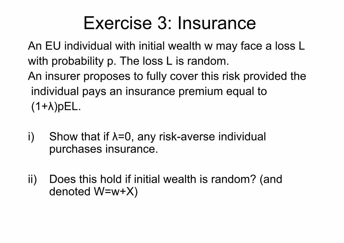
Exercise 3: InsuranceAn EU individual with initial wealth w may face a loss Lwith probability p. The loss L is random. An insurer proposes to fully cover this risk provided theindividual pays an insurance premium equal to(1+λ)pEL.

i) Show that if λ=0, any risk-averse individualpurchases insurance.

ii) Does this hold if initial wealth is random? (and denoted W=w+X)

More Risk Aversion?

• A risk neutral individual: u linear• A risk averse individual: u concave• How to characterize a « more risk averse »

individual?

Risk-Aversion ‘in the Small’

• Eu(w+kX)=u(w- π[k]) with X a pure riskand u twice differentiable

• Compute the approximation of the riskpremium: π[k] ~ π[0] + kπ’[0] + 0.5k2 π’’[0] = 0.5k2π’’[0] = 0.5k2EX2(-u’’(w)/u’(w))

Risk-Aversion ‘in the Large’?

• We want a measure of the intensity of risk-aversion for any risk (not only small ones).

• Does not exist!

• But there is the following fundamentaltheorem about comparative risk aversion

Pratt (1964, Etca)’s TheoremTheorem: The three following statements areequivalent. For all w and X,

i) -u’’(w)/u’(w) ≤ -v’’(w)/v’(w)ii) For all pure risks X, π[u,X] ≤ π[v,X] (larger risk

premium)iii) There exists an increasing and concavetransformation function T such that v(w)=T(u(w))

An individual with a vNM v is said to be more risk-averse than u iff -u’’(.)/u’(.) ≤ -v’’(.)/v’(.)

Risk Tolerance and DARA

Definition: Risk Tolerance is the reciprocal ofrisk aversion, that is -u’/u’’

Definition: Relative Risk Aversion: -zu’’(z)/u’(z)

Definition: A utility function u(.) displays Decreasing(resp. Increasing) Absolute Risk Aversion, denotedDARA (resp. IARA), iff -u’’(w)/u’(w) is decreasing(resp. increasing) in w

DARA more intuitive

Exercises• Exercise 4. Individual V is more risk-averse

than individual U, and both have the sameinitial wealth. Show that individual V rejects all lotteries that individual U rejects.

• Exercise 5. Show that DARA implies i) u’convex, and ii) that u less risk-averse than -u’

Some Utility FunctionsLinear: wQuadratic: -(a-w)2; 0≤w≤aExponential: -Exp(-aw); a≥0; (coined CARA)Logarithmic: Log(w)CRRA: (w)1-g/(1- g) with g≥0HARA: a(b+w/g)1-g with b+w/g≥0

• Exercise 6: Compute the Arrow-Pratt’scoefficient for these utility functions; Check whether DARA or not; check that HARA has linear risk tolerance

Risk-aversion vs. Risk

• Pratt’s theorem: keep the risk the same and compare different individuals (different utility functions)

• Help define the meaning of « more risk-averse » (Arrow-Pratt coefficient)

• From now, let’s keep the individual the same, but change the level of risk

• Define the meaning of « more risk »

« More Risk » - An Example• Which one of the two lotteries do you

prefer?X1 = (25%,300; 25%, 100; 25%, 0; 25%, -200)X2 = (50%, 200; 50%,-100),

• Show that any risk-averse EU maximizerprefers X2 to X1

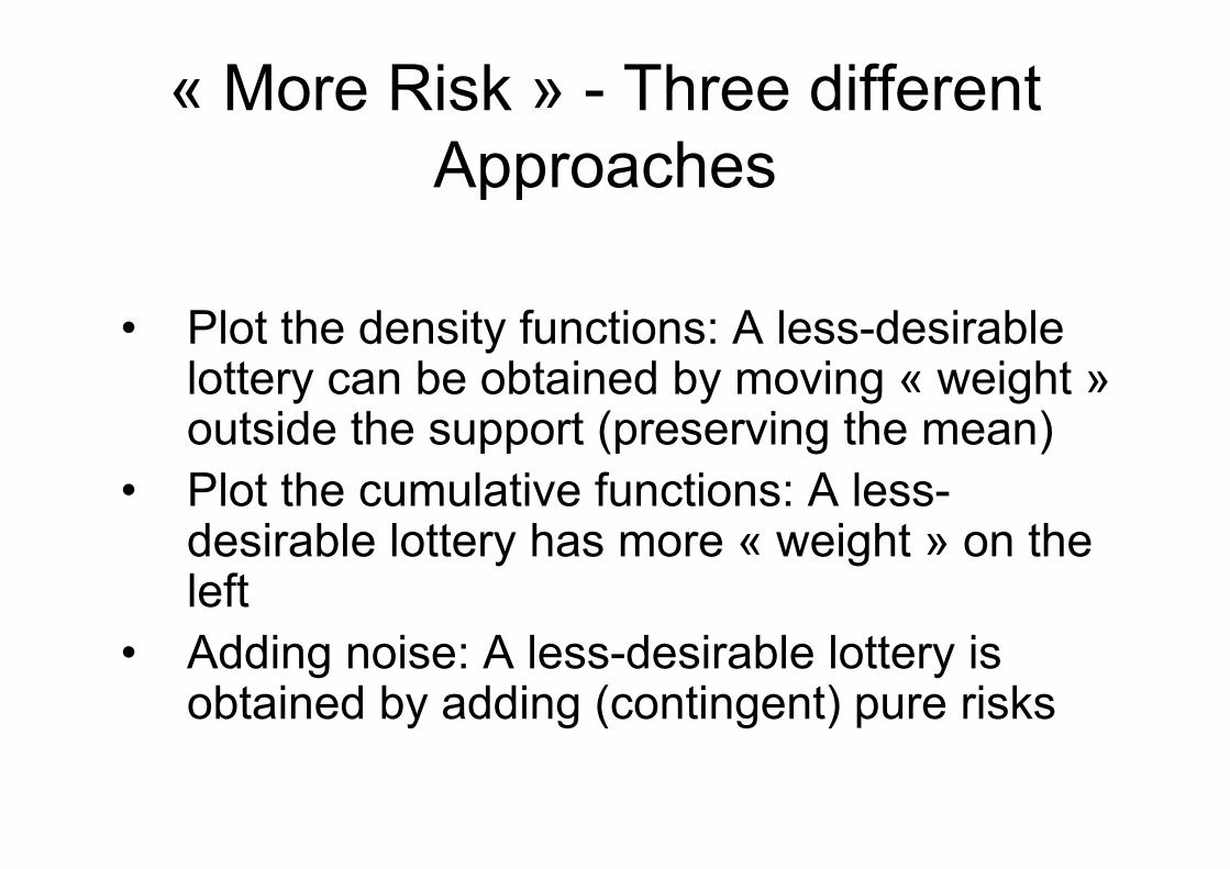
« More Risk » - Three differentApproaches

• Plot the density functions: A less-desirablelottery can be obtained by moving « weight »outside the support (preserving the mean)

• Plot the cumulative functions: A less-desirable lottery has more « weight » on the left

• Adding noise: A less-desirable lottery isobtained by adding (contingent) pure risks

Stochastic Dominance

Definition: Let F1 and F2 denote two cumulative distributions of X1 and X2 over support [a,b]. X2 dominates X1 in the sense of the second orderstochastic dominance (denoted X2 SSD X1) iff

Definition (more common): A SSD that preservesthe mean (D(b)=0) is called a « decrease in risk »

[ ]2 1D( ) ( ) ( ) 0 for all t

at F s F s ds t= − ≤∫

(Notice that: (Xi) ( ) )b

ia

E b F s ds= −∫

Decrease in RiskTheorem (Rothschild and Stiglitz, JET, 1970-71)The three following conditions are equivalent:

i) X2 is a « decrease in risk » of X1 (definition)ii) Eu(X2) ≥ Eu(X1) for all u concaveiii) X1 is obtained by adding (contingent) pure

risks to X2

Proof(See RS 1970, Ingersoll 1987, p 137)

Sketch of the proof:ii) equivalent to iii) : use Jensen’s inequalityii) equivalent to i) : start with ii) and make two

successive integrations by parts

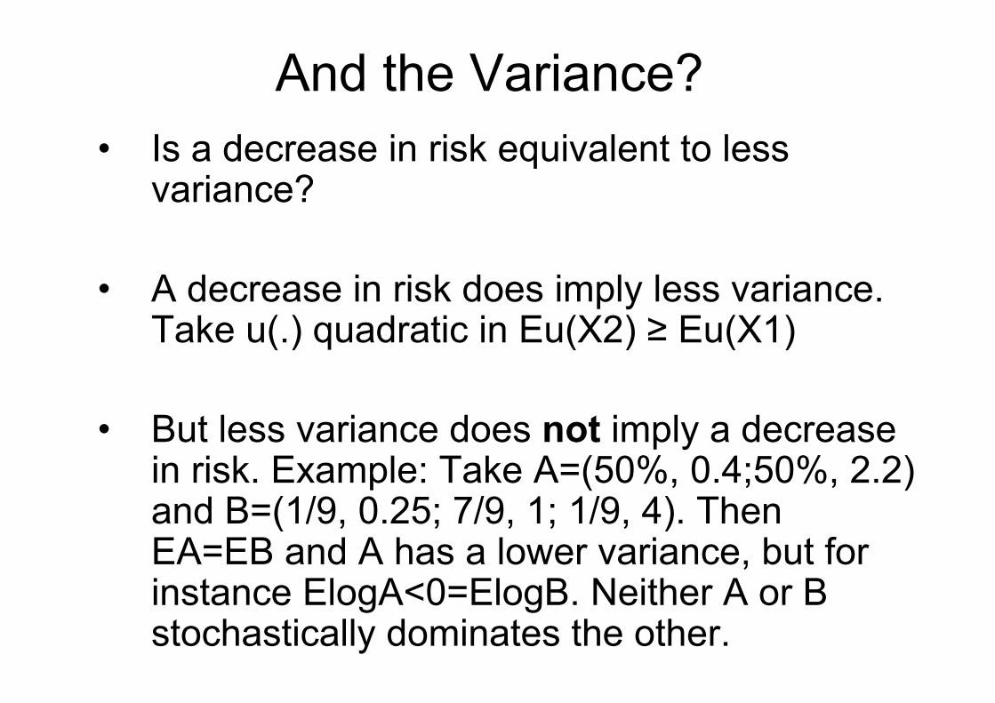
And the Variance?• Is a decrease in risk equivalent to less

variance?

• A decrease in risk does imply less variance. Take u(.) quadratic in Eu(X2) ≥ Eu(X1)

• But less variance does not imply a decreasein risk. Example: Take A=(50%, 0.4;50%, 2.2) and B=(1/9, 0.25; 7/9, 1; 1/9, 4). ThenEA=EB and A has a lower variance, but for instance ElogA<0=ElogB. Neither A or B stochastically dominates the other.

First-Order Stochastic DominanceTheorem: The three following conditions areequivalent:

i) X2 FSD X1 (definition)ii) Eu(X2) ≥ Eu(X1) for all u increasingiii) F1(t) ≥ F2(t) for all t

Exercise 7: Proof (hint: similar to the proof of the Rothschild andStiglitz’s theorem? Just one integration by part)

Meaning of First-Order StochasticDominance (FSD)

• X2 is « unambiguously » better than X1 • For every outcome t, the probability of

getting at least t is higher under F2 thanunder F1.

• Remark: the cumulative functions must not cross

More on FSD/SSD

• Mas-Colell et al., 1995 – pages 194-99• Gollier, 2001 – pages 39-48• Hirshleifer and Riley, 1994 – pages 105-

119• Ingersoll, 1987 – pages 136-38

Main Limits of FSD/SSD

• Incomplete orderings (just a subset of random variables can be ordered)

• Not able to characterize the level of «riskiness » of a single random variable

• Needs an index of risk, that would parallelthe Arrow-Pratt’s index of risk aversion

• A good index should both increase withmore dispersion (SSD), and a lowerlocation (FSD)

Some Possible Indexes• Variance – but does not depend on location • Entropy (∑kpkLog2pk) – only depends on

probabilities, does not depend on outcomes: absurd!

• (Inverse of the) Sharpe ratio (mean/standard deviation) – violates FSD

• Value at risk at x% (greatest possible lossignoring losses with proba less than x%) –arbitrary paramater x, ignores the gain side of the lottery, violates FSD

• Index of riskiness

Aversion to Downside RiskDefinition: An agent is averse to a downside

risk iff he always prefers that a pure risk iscontingent to a good outcome rather thancontingent to a bad outcome

Theorem (Menezes et al., 1980, AER): An EU individual is averse to a downside risk iff hisvNM utility u(.) is such that the marginal utility u’(.) is convex

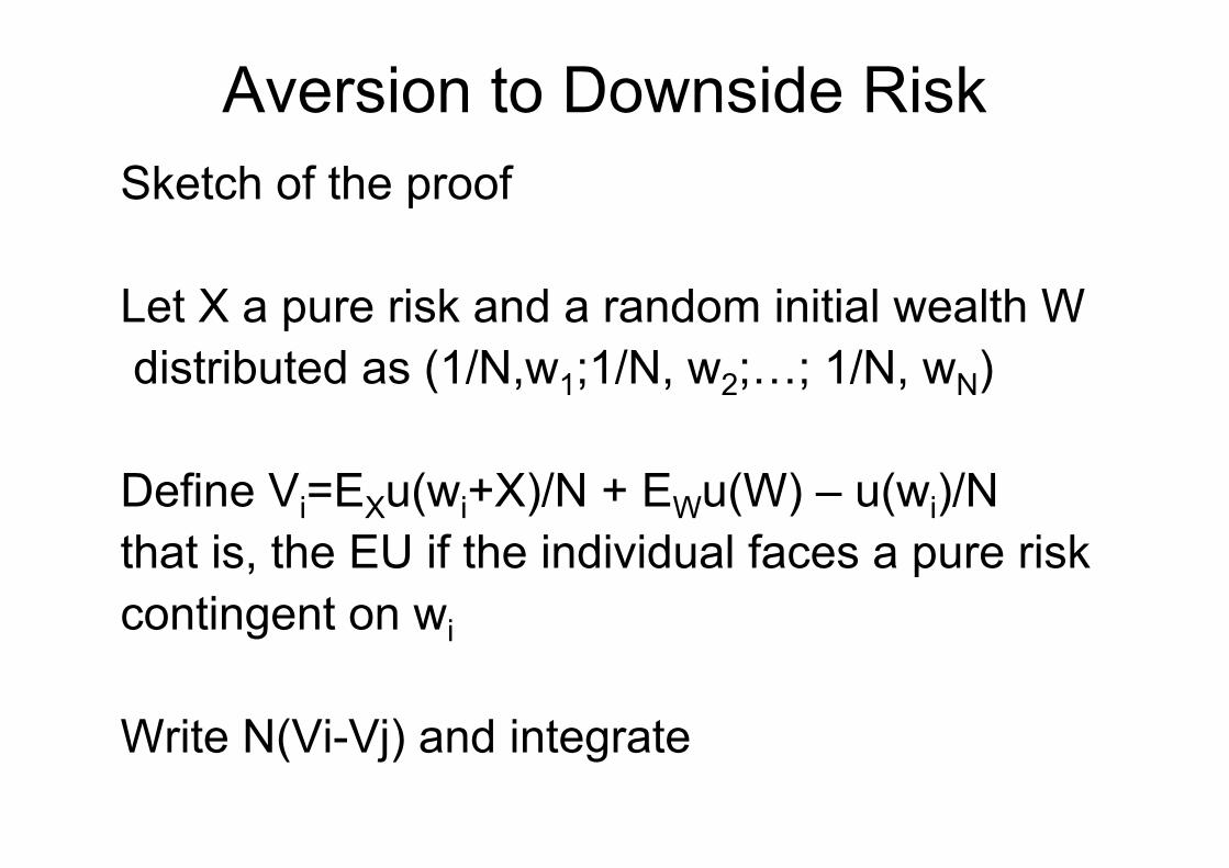
Aversion to Downside RiskSketch of the proof

Let X a pure risk and a random initial wealth Wdistributed as (1/N,w1;1/N, w2;…; 1/N, wN)

Define Vi=EXu(wi+X)/N + EWu(W) – u(wi)/Nthat is, the EU if the individual faces a pure riskcontingent on wi

Write N(Vi-Vj) and integrate

Information• Information is an important way to cope with risk –

Allows the decision-maker to adapt decisions to a better knowledge of risk

• Information is obtained from: information search, the passage of time, scientific progress, education, media, social interactions…

• In what follows, information will be- exogenous (e.g., no learning by doing)- non-strategic- free

Example: Investment DecisionCost: c, Benefit: X (uncertain). Risk-neutrality.

Investment rule: invest if EX>c ; Expected profit: max(EX-c, 0)

Suppose now perfect information.Investment rule: invest if X=x>c ; Expected profit: Emax(X-c,0)

Information Value: IV=Emax(X-c,0) - max(EX-c, 0) ≥0

Take: c=100, X=(50%, 200, 50%, 50). IV= 50-25=25Take: c=100, X=(50%, 140, 50%, 50). IV= 20-0=20

The Concept of Information• Information, as defined in economics, means

that the decision-maker will receive a message about the realisation of X

• The value of information is computed ex ante., i.e. before any message is received. Hence, the decision-maker does not know whichmessage (about the realization of X) will come.

=> The information value is always positive

Positive Information Value

• Let u(d,X) any decision problem in which d is the decision and X a random variable

• Value of informationIV= E maxd u(d,X) – maxd Eu(d,X)

Show that IV is always positiveIntuition?

Remark: Information Value

• Can be shown that IV is positive iff EU• Value of perfect information: full information

versus no information• In economics and statistics: « Better

information » is characterized using the Blackwell (1951)’s notion of the comparisonof information structures

Information and Time

• Information is important in a sequentialdecision-making framework

• What should I do today given that I willhave better information in the future?

• Should I wait? Should I delay decisions? Should I be more cautious?

• Debates around the PrecautionaryPrinciple

Exercise 8: Park vs. parking• Consider the choice between preserving a park and

building a parking • There are two periods (present and future), and the

discount rate is assumed to equal zero (to simplify)• The costs and benefits have been estimated by our best

experts• The park yields $0 in period 1, and either $100 or $0 in

period 2 with equal probability (it may contain a rare specie with high medecine value to be potentiallydiscovered in the future with probability 1/2)

• The parking yields $40 in each period, and costs $25• Based on economic analysis, the parking is built (since it

yields $55 which is higher than the expected return of the park $50)

• Do you agree with this choice in favor of the irreversibledecision?

3. Choice in Risky Situations

Outline- The standard portfolio model- Insurance demand- Savings- Prevention

The Standard Portfolio Model

• The standard portfolio model is the paradigmatic model for analyzing risk-taking• Idea: Examine the portion of the risk the decision-maker wants to bear• Technically: The risk is multiplicative• This model is at the root of capital assetpricing models (CAPM)

The Standard Portfolio Model

• An agent maximizes a strictly increasing, concave and thrice differentiable vNM utility function u. • Initial wealth is w0

• There exist only two assets: a riskless asset withrate of return r, and a risky asset with random rate of return R • The agent can invest an amount a (with a≤w0) in the risky asset, and (w0-a) in the riskless asset

The Standard Portfolio Model

Eu((w0-a)(1+r)+a(1+R)) = Eu(w0(1+r)+a(R-r)),

that will be denoted Eu(w+aZ) where Z=R-r isthe « net » return of the risky asset

Objective: examine the optimal risk-takingdecision: a*

FOC: EZu’(w+a*Z)=0 SOC: EZ2u’’(w+aZ)<0 under strict concavity of u

Interiority Condition

FOC: EZu’(w+a*Z)=0

Exercise 1: Show that a*>0 if and only if EZ>0Sketch of the proof: Let g(a)= Eu(w+aZ) ; Compute g’(0)

Remark: if Z is always positive (resp. negative) then a* is equal to w0 (resp. 0)

We will assume throughout that a* is interior: 0<a*<w0

Small Risk ‘Heuristics’

Let Z ‘small’ compared to w so that:Eu(w+aZ)#u(w)+a(EZ)u’(w)+0.5a2(EZ2)u’’(w)

Maximizing over a the last expression leads toa*=(EZ/EZ2)(-u’(w)/u’’(w))

Increase in EZ, decrease in Var(Z), increase in risk tolerance -u’(w)/u’’(w): intuitive effects

Exercise 2: Show that the above approximation is correct for u quadratic

Risk-aversion: Exercises

Exercise 3: Show that an increase in risk-aversion always leads to decrease a*

Exercise 4: Show that if the utility function isCRRA, a* is proportional to wealth w.

Exercise 5: Show that, under DARA, an increase in wealth w leads to increase a*

Change in Risk

• Unlike the effect of more risk aversion, the effectof more risk in the sense of RS is ambiguous

• That is, it is not true in general that an increase(resp. decrease) in risk of Z leads to decrease(resp. increase) a* for any risk-averse investor

• This is true, however, for some particular types of decrease in risk, for some probability distributions, and some utility functions (see, e.g., small risks, quadratic utility function; see Gollier 2001)

Empirical Observations

• Most people do not have any risky asset in their portfolio, only about 20% do have (« stock participation puzzle »)

• Rich people invest relatively more than poorpeople in risky assets. The equity share is not constant. See, e.g., Guiso et al. (AER 1996)

The Equity Premium Puzzle

• Need « extremely » high risk aversion to explain the equity premium (g>40)

• Mehra and Prescott (JME, 1985) and a voluminous subsequent literature

• Explanations?

Insurance

An agent faces the risk of losing L (random) if an accident occurs: Eu(w0-L)

Insurance contract: get αL if accident, pay an insurance premium P=(1+λ)αEL (where λ is an insurance loading factor, 0≤α≤1)

Eu(w0- L+ αL - (1+λ)αEL)= Eu(w0-(1+λ)EL+(1- α)((1+λ)EL-L))

Insurance

Eu(w0-(1+λ)EL+(1- α)((1+λ)EL-L))=Eu(w+aZ)where w=w0-(1+λ)EL, a= (1- α) and Z=(1+λ)EL-L

• The choice a corresponds to the risk retentionon the insurance market

• Observe that EZ= λEL

Insurance

• Theoretical Predictions:

Using the standard portfolio model (see before):1) a*>0 iff EZ>0 α*<1 iff λ>0 (full insurance

not optimal)2) DARA, a* increases with wealth w α*

decreases with wealth w

Empirical Puzzles in Insurance

• Inconsistent with theory:

1) Full insurance policies are prevalent2) Insurance has often been found to be a normal good (increases with wealth)

• Explanations?

Firm’s Production

Exercise 6: Let the problem maxqEu(Pq-c(q)) with uncertain price P>0 and with c’’(q)>0

i) Characterize FOC, SOCii) Show that optimal production under certainty, and under risk-neutrality are identicaliii) Compare to arg maxqEu(Pq-c(q))iv) Show, more generally, that an increase in risk-aversion reduces production under priceuncertainty

SavingsOutline

- A simple two-period model- The notion of « prudence »- How large are precautionary savings?- Recursive preferences

Two-Period ModelU(c1,c2)=u(c1)+bv(c2) where b is a discount factor

Assume u, v strictly increasing and concave and thrice differentiable

y1, y2 : income in period 1 and 2

Budget constraint: ρy1+y2= ρc1+c2

where ρ is the interest factor (one plus the interestrate)

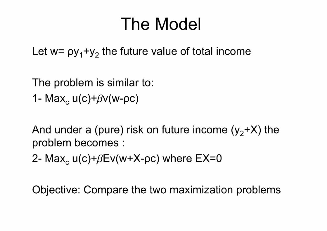
The ModelLet w= ρy1+y2 the future value of total income

The problem is similar to: 1- Maxc u(c)+bv(w-ρc)

And under a (pure) risk on future income (y2+X) the problem becomes :2- Maxc u(c)+bEv(w+X-ρc) where EX=0

Objective: Compare the two maximization problems

FOC,SOCCertainty:FOC: u’(c*)-bρv’(w-ρc*)=0SOC: u’’(c)+bρ2v’’(w-ρc)<0

Uncertainty:FOC: u’(c**)-bρEv’(w+X-ρc**)=0SOC: u’’(c) + bρ2Ev’’(w+X-ρc)<0

Precautionary savings= c*-c**= reduction in currentconsumption due to a future income risk(Assume interiority)

Precautionary SavingsAre precautionary savings positive?Intuitively: Yes, under risk-aversion. Wrong!

Formally: True if for all b, ρ, w and Xu’(c*)-bρEv’(w+X-ρc*) ≤ 0 = u’(c*)-bρv’(w-ρc*)

Equivalent to: for all z and X, Ev’(z+X)≥v’(z+EX)

Precautionary SavingsFor all X, Ev’(z+X) ≥v’(z+EX)By Jensen <=> v’ convex, or v’’’≥0

Not risk-aversion, but aversion to downside risk

This condition, v’’’ ≥0, is commonly known as the condition of « prudence » (Kimball, 1990, Etca)

Early literature: Leland (1968, QJE)

IntuitionWhat matters is not how risk « hurts » utility (risk-aversion) … but how risk « hurts » marginal utility of income (« prudence »)

Prudence: one unit of wealth has more value under uncertainty

Aversion to a downside risk : uncertainty has more negative impact when less wealthy

Remark: Multiperiod

Let the indirect utility function:U(w)=Maxc u(c)+bu(w-ρc).

If u risk-averse (resp. prudent) then U is risk-averse (resp. prudent) as well.

This suggests that the results can usually beextended to multiperiod.See Caroll and Kimball (1996, Etca)

Remark: Increase in Risk

Can be extended to any increase in risk in the sense of Rothschild and Stiglitz (1970).

Depends on whether f(x)=u’(c)-bρv’(w+x-ρc) isconcave in x for all the values of the parameters=> prudence

How Large are PrecautionarySavings?

• Controversies

• Dynan (1993, JPE) find little evidence for precautionary savings. Relative prudence - i.e., formally -xv’’’(x)/v’’(x) - is estimated to be equal to #0.3 => very small and inconsistent with CRRA utility function

• In contrast, Guiso et al. (JME) and Caroll and Samwick (1998, REStat) find significant precautionarysavings motive

Capital riskExercise 7 Let Maxc u(c)+bERv(R(y1-c)) where Ris random (capital) risk.

i) Examine the effect of more capital risk on consumption

ii) Compare the NS condition to that of prudence. Discuss.

A Conceptual Caveat- u(c1)+bu(c2) : the curvature of u captures the desire to smooth consumption across time (elasticity of substitution) under certainty

- Eu(C) : the curvature of u captures risk-aversion, i.e. captures the desire to smoothconsumption across states of nature in a staticmodel

=> Not clear why these two different concepts are linked through the same utility function u(.)

Recursive PreferencesPermit to disentangle the two concepts : Kreps and Porteus (1978, Etca), Selden (1978, Etca), Epstein and Zin (1989, Etca)

=> « Recursive preferences »

Built in two different steps:

1) Let f=v-1(Ev(C2)) the certainty equivalent of uncertainperiod 2 consumption C2: atemporal context

2) Let u(c1)+bu(f) the intertemporal preferences w/r to the flow of deterministic consumption: certainty context

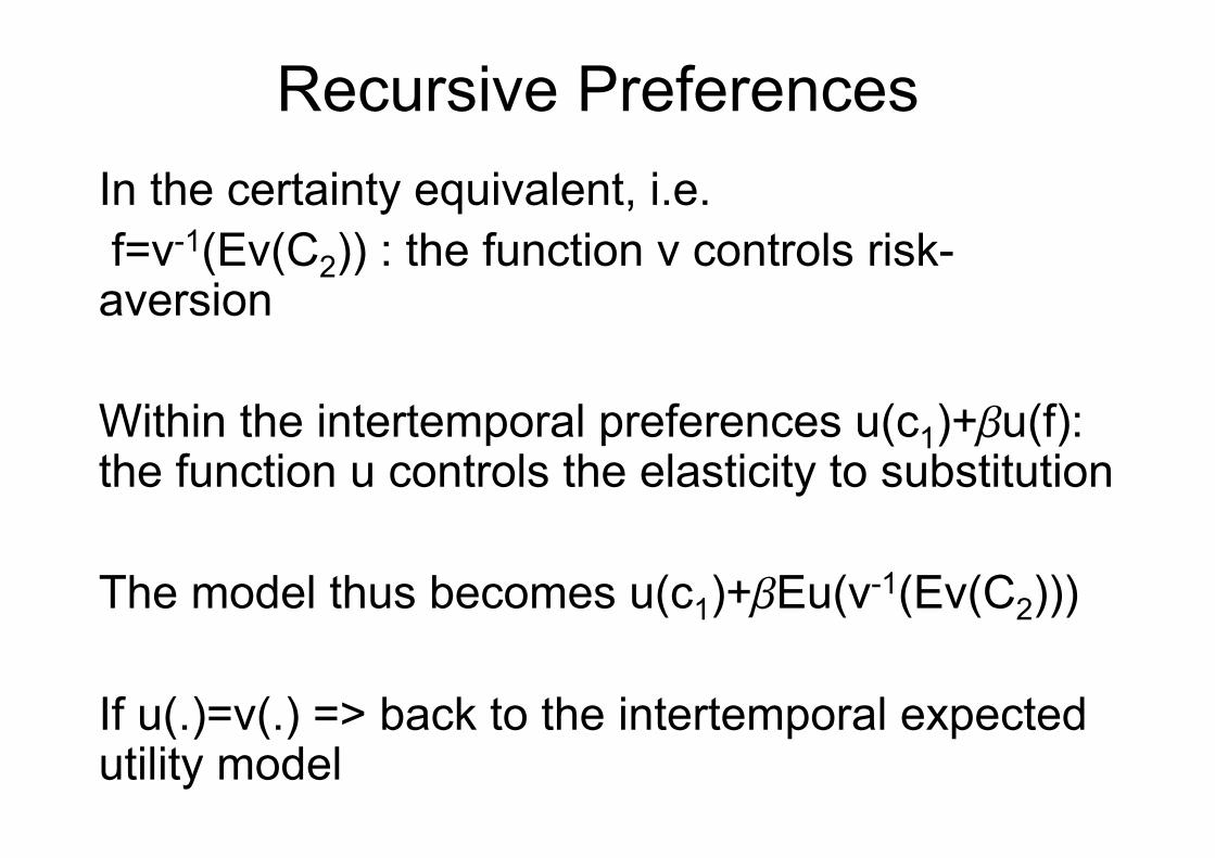
Recursive PreferencesIn the certainty equivalent, i.e.f=v-1(Ev(C2)) : the function v controls risk-aversion

Within the intertemporal preferences u(c1)+bu(f): the function u controls the elasticity to substitution

The model thus becomes u(c1)+bEu(v-1(Ev(C2)))

If u(.)=v(.) => back to the intertemporal expectedutility model

Empirical DataEpstein-Zin (1991, JPE) examine consumption-portfolio choices under recursive preferences withv(z)= (z)1-g/(1-g) and u(z)= (z)1-α/(1- α)

Reject the assumption that g=α ! (i.e., reject EU)

Elasticity of substitution (1/α ): α in range [2.4,4.8]Relative risk-aversion: g in range [0.4,1.4]

Some Other Estimates

0.5-4.5>7Kocherlakota(1996)

0.25#1Chavas and Thomas (1998)

1.2-3.00.4-3.6Normandin, St Amour (1996)

0.4-1.4#1Giovanni, Jorion (1991)

1045Weil (1990)

αgParameters:References:

PreventionOutline:- Self-insurance- Self-protection- State-dependent utility- WTP vs. WTA- Value of statistical life

Self-insurance

• Reduction of the size loss if an accident occurs

• A simple self-insurance decision model :Maxe (1-p)u(w-e) + pu(w-e-L(e)) with– p: probability of loss, e: self-insurance effort– L(e): loss, with L(.)>0, L’(e)<-1, L’’(.)>0– w: initial weath, u(.): vNM utility function, with

u’(.)>0 and u’’(.)≤0

Self-insurance and Risk Aversion• First order condition

g(e) = -(1-p)u’(w-e) + p(-1-L’(e))u’(w-e-L(e)) = 0• Under risk neutrality

-1-pL’(e*) = 0

• Risk aversion increases effort e iff g(e*)≥0g(e*)= (1-p)(u’(w-L(e*)-e*)-u’(w-e*)) ≥0

• Holds true. Risk averse agents thus invest more in self-insurance than risk neutral agents

ee*

RN utility

RA

Self-protection

• Reduction of the probability of the loss• A simple self-protection decision model:

Maxe (1-p(e))u(w-e) + p(e)u(w-L-e) with p(.)∈[0,1], p’(.)<0 and p’’(.)>0

• First order conditiong(e) = -p’(e)(u(w-e)-u(w-L-e)) - (1-p(e))u’(w-e) -p(e)u’(w-L-e) = 0

Self-protection and Prudence

• Risk aversion may decrease, and not increase, self-protection (Dionne and Eeckhoudt 1985 EL)• Eeckhoudt and Gollier (2005 ET) show that a riskaverse, and prudent, agent should invest less, and not more, in prevention than a risk-neutral agent!• Intuition: aversion to a downside risk• Consider two lotteries:

A B3,000

1,000

2,000

0

1/4

3/4

3/4

1/4Same mean and variance

State-Dependent Utility• Until now, we have assumed that the utility was state-independent: No matter the « state of the world », same vNMutility u(.)

• Sometimes irrealistic to assume state-independence

• The utility function may depend on the « state of the world »

• Assume two states: either I will be alive (state 1), or dead(state 2)

• The utility of wealth should probably be allowed to bedifferent depending on the state of world

Some referencesOn state-dependent utility

Fishburn, P., 1970, Utility Theory for Decision-Making, Wiley. New York.

Karni, E., 1985, Decision Making under Uncertainty, Harvard UP.

Keeney R. and H. Raiffa, 1993, Decisions with Multiple Objectives, Cambridge UP.

A Prevention ModelThere are two states of the world, the good state and the bad state

• u(w) is utility of wealth w in the good state• v(w) is utility of wealth w in the bad state (e.g., if sick or dead)

Assume u(w)>v(w) and u’(w)>0, v’(w)≥0 for all w.

A Prevention Model (cont’d)Let 0≤p(e)≤1 the probability that the bad state occurs in which e is the prevention effort (in monetary units) with p’(e)<0 and p’’(e)≥0.

Under (state-dependent) EU, we have:EU=(1-p(e))u(w-e)+p(e)v(w-e)

See, e.g., Weinstein et al. (1980, QJE), Viscusi(1993, JEL)

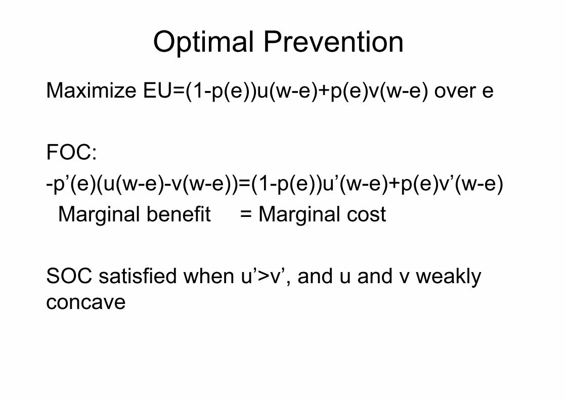
Optimal PreventionMaximize EU=(1-p(e))u(w-e)+p(e)v(w-e) over e

FOC: -p’(e)(u(w-e)-v(w-e))=(1-p(e))u’(w-e)+p(e)v’(w-e)Marginal benefit = Marginal cost

SOC satisfied when u’>v’, and u and v weaklyconcave

What is the Shape of v(.)?Some particular cases:

• v(w)=u(w-L) monetary loss, state-independent, self-protection model

• v(w)=u(w)-k additive separability, strong assumption = samemarginal utility of wealth

• v(w)=ku(w) with 0≤k<1 e.g., if k=0, utility if dead with no bequest motiveViscusi and Evans (1990, AER) estimate k#0.7

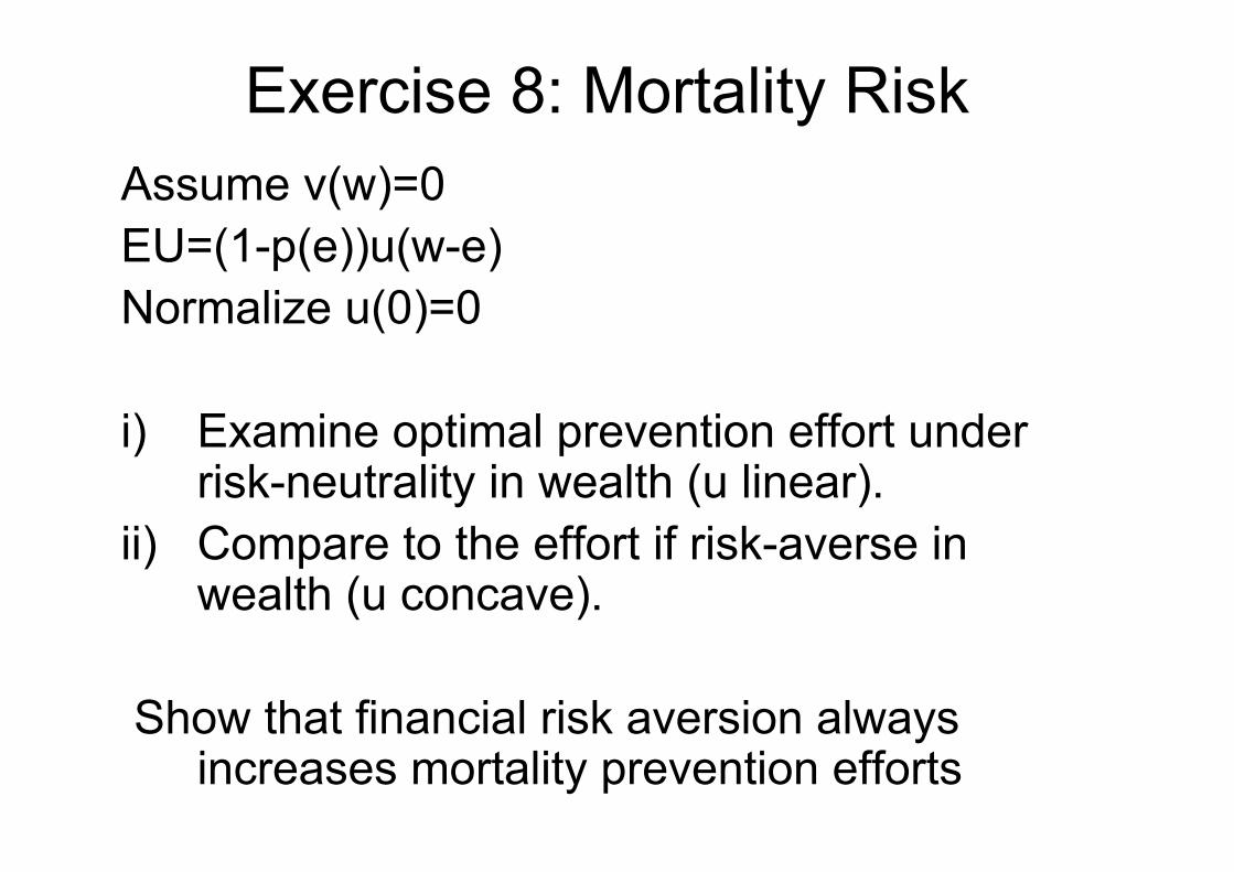
Exercise 8: Mortality RiskAssume v(w)=0EU=(1-p(e))u(w-e)Normalize u(0)=0

i) Examine optimal prevention effort underrisk-neutrality in wealth (u linear).

ii) Compare to the effort if risk-averse in wealth (u concave).

Show that financial risk aversion alwaysincreases mortality prevention efforts

Valuation of Mortality RiskReduction

• Important policy issue• Suppose one wants to implement a

public project that is expected to savelives in the society (e.g., reducepollution)

• What is the social value of this project?• How to compare this benefit to the

monetary cost of the project?

Willingness to Pay

• In our context: maximal amount that an individual is willing to pay for a mortality risk reduction

• Theoretically: The amount that keeps constant the level of expected utility

Russian Roulette • Pure thought experiment!• The gun has 10,000 chambers, and 5 of them are

loaded with bullets• You are given the opportunity to remove one bullet

before shooting. What is your WTP for this removal?

(1-p+e)u(w-WTP) + (p-e)v(w-WTP) = (1-p)u(w) + pv(w)

with p=5/10,000 et e=1/10,000w= initial wealthu(.) utility if alive; v(.) utility if dead

WTP/WTA

• WTA — Willingness to Accept (Russian Roulette: Which amount would

you accept to add one more bullet?)

• WTP is limited by available wealth; WTA not limited

– Usually WTP ≤ WTA– For small amounts, WTP ≈ WTA

WTP/WTA

Indifference curve

Wealth

0 Survival probability ( = 1 - risk) 1

WTP/WTA

Indifference curve

WTP

Wealth

0 Survival probability ( = 1 - risk) 1

Δp

WTP/WTA

Indifference curve

WTA

WTP

Wealth

0 Survival probability ( = 1 - risk) 1

Δp

Δp

Value of Statistical Life (VSL)

• N (= 10,000) identical citizens in a community • A public project may save one statistical life• WTP equals 500 euros for the risk reduction

project (of 1/10,000 per individual)• VSL is thus 5 million euros total within this

community

• ( )_VSL_

WTP N WTP Total WTPp N p E Life saved

⋅= = =

Δ ⋅ Δ

Introduction to the concept:

VSL : Theory

( )d w u (w ) v (w )V S Ld p 1 p u '(w ) p v '(w )

−= =

− +

Let V=(1-p)u(w) + pv(w)VSL: marginal rate of substitution between

money and risk

VSL

• Does not measure what an individual is willing to pay to avoid his/her own death with certainty

• It measures WTP (resp. WTA) for an infinitesimal risk reduction (resp. increase)

VSL :i) Increases with baseline risk p (“dead-anyway

effect”, Pratt and Zeckhauzer, 1997, JPE)ii) Increases with wealth w (the sum of two

effects) under u and v weakly concave

Author Year Implicit VSL Countrymillions US $2000

• WAGE DIFFERENTIAL STUDIES• Thaler-Rosen 1975 $1.0 US• Viscusi 1978-79 $5.3 US• Dillingham 1977 $3.2-$6.8 US• Weiss et al. 1981 $3.9-$4.5 Austria• Marin et al. 1982 $4.2 UK• Moore-Viscusi 1988 $3.2-$6.8 US• Berger-Gabriel 1991 $8.6-$10.9 US• Cousineau et al. 1992 $2.2-$6.8 Canada• Leigh 1995 $8.1-$16.8 US• Baranzini et al. 2001 $6.3-$8.6 Switz.• Kim 1993 $0.8 India• Liu et Hammitt 1997 $0.2-$0.9 Taiwan

• CONSUMER-MARKET STUDIES• Blonquist 1979 $1.0 US• Atkinson-Alvorsen 1990 $5.3 US• Dreyfus-Viscusi 1995 $3.8-$5.4 US

• CONTINGENT VALUATIONS• Johannesson et al. 1996 $5.0 Sweden• Corso et al. 2001 $3.1 US• Ludwig-Cook 2001 $6.0 US

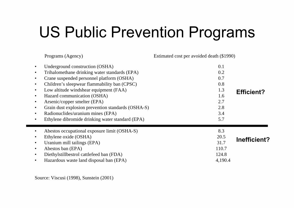
US Public Prevention ProgramsPrograms (Agency) Estimated cost per avoided death ($1990)

• Underground construction (OSHA) 0.1• Trihalomethane drinking water standards (EPA) 0.2• Crane suspended personnel platform (OSHA) 0.7• Children’s sleepwear flammability ban (CPSC) 0.8• Low altitude windshear equipment (FAA) 1.3• Hazard communication (OSHA) 1.6• Arsenic/copper smelter (EPA) 2.7• Grain dust explosion prevention standards (OSHA-S) 2.8• Radionuclides/uranium mines (EPA) 3.4• Ethylene dibromide drinking water standard (EPA) 5.7

• Abestos occupational exposure limit (OSHA-S) 8.3• Ethylene oxide (OSHA) 20.5• Uranium mill tailings (EPA) 31.7• Abestos ban (EPA) 110.7• Diethylstillbestrol cattlefeed ban (FDA) 124.8• Hazardous waste land disposal ban (EPA) 4,190.4

Source: Viscusi (1998), Sunstein (2001)

Efficient?

Inefficient?