ecosystem assessment of mountain ash forest in the … · ecosystem assessment of mountain ash...

Ecosystem assessment of mountain ash forest in theCentral Highlands of Victoria, south-eastern Australia

EMMA L. BURNS,1,2* DAVID B. LINDENMAYER,1,2,3,4 JOHN STEIN,1

WADE BLANCHARD,1 LACHLAN MCBURNEY,1,2 DAVID BLAIR1,2 ANDSAM C. BANKS1

1Fenner School of Environment and Society, The Australian National University, Canberra, ACT 0200,Australia (Email: [email protected]), 3ARC Centre of Excellence for Environmental Decisionsand 4National Environmental Research Program, The Australian National University, and 2Long TermEcological Research Network, Terrestrial Ecosystem Research Network, Canberra, Australian CapitalTerritory, Australia

Abstract We applied an ecosystem risk assessment to the mountain ash forest ecosystem of the CentralHighlands of Victoria (hereafter ‘mountain ash forest’), south-eastern Australia, using the IUCN Red List ofEcosystems criteria. Using this methodology, we quantified: (i) key aspects of the ecosystem’s historical, currentand future decline in spatial distribution; (ii) the extent of occurrence and area of occupancy for the mountain ashecosystem; and (iii) the decline in key abiotic and biotic processes and features for historical, current and futuretime periods. We developed a probabilistic model of tree growth stages to estimate the risk of ecosystem collapsewithin 50 to 100 years in the mountain ash forest.There was uncertainty in our estimates of risk under the variousIUCN criteria, with two sub-criteria being categorized as ‘Data Deficient’. Our overall ranking of risk of collapsefor the ecosystem was Critically Endangered.We are confident that this risk category is appropriate because all 39scenarios modelled indicated a ≥92% chance of ecosystem collapse by 2067. Our findings highlight the importantneed for timely policy reform to facilitate improved management of the mountain ash ecosystem in Victoria. Inparticular, there needs to be greater protection of remaining areas of unburned forest, and restoration activities inparts of the forest estate. Implementation of these strategies will require a significant reduction in logging pressureon the mountain ash ecosystem.

Key words: climate, ecosystem collapse, fire, logging, mountain ash.

INTRODUCTION

The mountain ash forest is a globally iconic ecosystem.Mountain ash is the world’s tallest flowering plant andindividual trees may reach 50 m height within 35 yearsof germination (Ashton 1975). They can eventuallyexceed 90 m after several hundred years with somespectacular trees over 100 m tall having been docu-mented (Beale 2007). The mountain ash forest ishighly valued for its contributions to water and timberproduction (Flint & Fagg 2007; Viggers et al. 2013),its recreational and aesthetic values, and itsunique biodiversity (see for example Mueck 1990;Lindenmayer 2009a). In addition to its unique species,the dynamics of the ecosystem are unusual amongAustralian forests because they can be subject tostand-replacing disturbance regimes such as wildfire(Lindenmayer et al. 2011a).

In this paper, we applied an ecosystem risk assess-ment to the mountain ash forest, using the Interna-tional Union for the Conservation of Nature’s (IUCN)Red List of Ecosystems criteria. The risk assessment

requires an assessment of five criteria, A-E, each(except E) with three sub-criteria. For each criterion,numerical thresholds define ordinal categories ofthreat from Least Concern (LC) through to CriticallyEndangered (CR) (Table 1).The final, overall rankingis determined by the most severe ranking of the fivecriteria (refer to the Methods section for further infor-mation, and Appendix S2 for a full explanation). TheIUCN developed these criteria to support a global RedList of Ecosystems, analogous to criteria that supportthe IUCN Red List of Threatened Species (IUCN2001).The IUCN Council formally endorsed the RedList of Ecosystems criteria in mid-2014, which was thefinal step after resolutions passed at two successiveWorld Conservation Congresses (in 2008 and 2012).The criteria are described by Keith et al. (2013), andan earlier paper by Rodríguez et al. (2011) providesfurther historical context. More recently, Nicholsonet al. (2014) compared the IUCN’s approach to thatused in Australia to assess the threat status ofecosystems/ecological communities within differentjurisdictions. Boitani et al. (2014) critiqued the crite-ria, arguing that species and ecosystems were notanalogues and the criteria were open to ambiguousinterpretations and uncertain outcomes. These are

*Corresponding author.Accepted for publication August 2014.

Austral Ecology (2014) ••, ••–••

bs_bs_banner

© 2014 The Authors doi:10.1111/aec.12200Austral Ecology © 2014 Ecological Society of Australia

mailto:[email protected]

noteworthy concerns, and we expect testing andrefinement will improve the criteria and how they areused. We apply the IUCN Red List of Ecosystemscriteria here to inform this process.

In applying the IUCN criteria to the mountain ashforest, we aimed to: (i) identify the defining features ofthe system and the processes that threatened them, (ii)evaluate trends in key variables relevant to the persis-tence of the ecosystem, and (iii) assess the risk ofecosystem collapse in the 21st century.

Ecosystem description

Characteristic native biota

Many areas of mountain ash forest are generally domi-nated by a single overstorey tree species – Eucalyptusregnans. Mountain ash forest can also contain otheroverstorey tree species like alpine ash (E. delegatensis)and shining gum (E. nitens) at higher elevations(Lindenmayer et al. 1993) or messmate (E. obliqua),mountain grey gum (E. cypellocarpa) and redstringybark (E. macrorhyncha) at lower elevations(Campbell 1984).

Mountain ash forest supports a wide range of plantspecies in the midstorey tree layer and shrub layers(Supporting Information Appendix S1), and a richarray of native mammals (Lumsden et al. 1991).Native mammals include the endangered Leadbeater’spossum (Gymnobelideus leadbeateri) which is virtu-ally confined to the Central Highlands region(Lindenmayer et al. 2014a) and the vulnerable yellow-bellied glider (Petaurus australis) as well as six otherspecies of arboreal marsupials and a diversity of forestbird species (Lindenmayer 2009a). Details of othernative vertebrate species are outlined in Appendix S1.

Classifications

According to the Victorian vegetation classificationsystem, mountain ash forest occurs within one Eco-logical Vegetation Class, ‘EVC 30 Wet Forest’ (http://www.dse.vic.gov.au/__data/assets/pdf_file/0010/98515/HFE_0030.pdf). Nationally, mountain ash forests areassigned to Major Vegetation Group 2, ‘Eucalypt Tall

Open Forests’ (Department of the Environment andWater Resources 2007). Under the IUCN HabitatsClassification Scheme (Version 3.1), mountain ashforests fall within habitat type 1.4, Temperate Forest.

Abiotic environment

Temperature and precipitation are the key abiotic vari-ables in the mountain ash ecosystem and, in general,climatic conditions are the key determinant of itsbroad distribution patterns (Lindenmayer et al. 1996).The climate is typically characterized by mild, humidwinters with occasional periods of snow, generally coolsummers, mean annual temperature varying from 7.2to 14.1°C and mean annual precipitation varying from815 to 1775 mm (long-term mean climate variablesestimated for the 1976 to 2005 period usingANUCLIM, Xu & Hutchinson 2013). Tree growththat is characteristic of the mountain ash forest canonly occur within the ‘wet and cool’ environmentalenvelope defined by the Central Highlands of Victoria(Lindenmayer et al. 1996; Mackey et al. 2002). Thisecosystem is therefore vulnerable to the effects ofclimate change, particularly higher temperatures andreduced rainfall (Nitschke & Hickey 2007; Wood et al.2014).

At finer spatial scales, other environmental factorssuch as soil fertility, topography and natural distur-bance also have an important influence on mountainash forest (Florence 1996; Lindenmayer et al. 1999;Mackey et al. 2002).The ecosystem typically occurs ataltitudes between 85 and 1380 m above sea level inmesic conditions favourable for tree growth (Mackeyet al. 2002).

The deep, well-drained soils typical of mountain ashforest are derived from Ordivician and Devonian sedi-ments, extrusives, granitic soils and alluvium. Some ofthe most fertile soils are deep red earths which overlayigneous felsic intrusive parent material. These have ahigh soil water holding capacity and nutrient availabil-ity compared with most forest soils in Australia(McKenzie et al. 2004).

Distribution

As discussed above, factors at multiple spatial scalesshape the distribution of the mountain ash forest.Thisecosystem occurs in a region approximately 120 kmnorth-east of Melbourne, south-eastern Australia(Fig. 1). Forests dominated by mountain ash alsooccur in north-eastVictoria, south-westernVictoria (inthe Otway Ranges) and throughoutTasmania (where itis also called swamp gum; Boland et al. 2006). Butseveral key aspects differentiate those forests from themountain ash ecosystem, including distinctive verte-brate fauna (Lindenmayer 2009a) and flora (Mueck1990).

Table 1. IUCN Red List ecosystem criterion for themountain ash ecosystem in the Central Highlands ofVictoria

Criterion A B C D E

Sub-criterion 1 LC EN DD CR CR(CR-CR)Sub-criterion 2 LC LC VU (LC-CR) CR (CR-CR)Sub-criterion 3 LC VU DD CR (CR-CR)

Sub-criteria with brackets indicate assessments undertaken using upperand lower bounds. CR, Critically Endangered; DD, Data Deficient; EN,Endangered; LC, Least Concern; VU, Vulnerable.

2 E. L. BURNS ET AL.

© 2014 The Authorsdoi:10.1111/aec.12200Austral Ecology © 2014 Ecological Society of Australia

http://www.dse.vic.gov.au/__data/assets/pdf_file/0010/98515/HFE_0030.pdf



The Central Highlands region supports approxi-mately 157 000 ha of mountain ash forest. Approxi-mately 20% is in closed water catchments, parts ofwhich are also managed as the Yarra Ranges NationalPark (Viggers et al. 2013). The remaining 80% islocated in areas broadly designated for paper pulp andtimber production (Flint & Fagg 2007; Lindenmayer2009a).

Key processes (threatening and natural) andtheir interactions

Fire is the primary form of natural disturbance inthe mountain ash ecosystem (Ashton 1981), andoverstorey trees are often killed in a high-severity con-

flagration (Smith et al. 2013).Young seedlings germi-nate from seed released from the crowns of burnedmature trees to produce a new even-aged regrowthstand. Lower severity fires can result in multi-agedstands when the fire stimulates a regeneration cohortbut is insufficiently intense to kill all overstorey trees(McCarthy & Lindenmayer 1998; Lindenmayer et al.2014b). Following disturbance and stand initiation,young mountain ash trees exhibit rapid rates ofgrowth.

The effects of fire on stand structure are linked tothe age of a forest at the time it is burned. Fire in anold growth forest will produce a cohort of large deadtrees and fire-scarred living old trees that can providenesting habitat for a suite of cavity-dependent species

Fig. 1. The distribution of mountain ash forests in the Central Highlands of Victoria (see Appendix S2 for data sources).

MOUNTAIN ASH ECOSYSTEM ASSESSMENT 3


such as Leadbeater’s possum (Lindenmayer 2009b).Such habitat does not develop in young burned forestbecause small diameter trees do not remain standinglong after they are burned, nor do they have the inter-nal volume of wood capable of supporting suitablysized cavities (Gibbons & Lindenmayer 2002). Whenthe interval between stand-replacing disturbances is<20 years – the period required for trees to reachsexual maturity and begin producing seed (Ashton1981) – stands of mountain ash will be replaced byother species, particularly wattle (Acacia spp.)(Lindenmayer et al. 2011a). Therefore, fires in rapidsuccession have the potential to eliminate populationsof fauna as a result of the direct effect they can have onfloristic composition (Lindenmayer et al. 2013).

Logging is the primary form of human disturbancein the ecosystem, and large areas have been subject totimber and pulpwood harvesting. Historically, moretimber flowed through Port Melbourne than ports likeSeattle in western North America, which have a fargreater area than Melbourne from which to sourcetimber (Dingle & Rasmussen 1991). In the past 40years, the conventional method of logging has beenclearfelling in which all merchantable trees within a15–40 ha area are cut in a single operation. Followingclearfelling, logging debris is burned to create a bed ofashes in which the regeneration of a new stand ofmountain ash takes place, often by artificial reseeding(Flint & Fagg 2007).

There are two kinds of important interactionsbetween natural disturbance (fires) and human distur-bance (logging) in the ecosystem. First, burned forestsare subject to salvage logging in which clearfellingoperations are employed in an attempt to recoversome of the economic value of fire-damaged trees(Lindenmayer et al. 2008). For example, widespreadsalvage logging occurred after wildfires in 1939, 1983and 2009 (Noble 1977; Lindenmayer & Ough 2006;Lindenmayer et al. 2010). Second, artificial standregeneration practices following conventionalclearfelling operations in green forest produce youngstands of dense regrowth forest. Recent quantitativeanalyses indicate that such stands are at risk ofre-burning at high severity (Taylor et al. 2014).

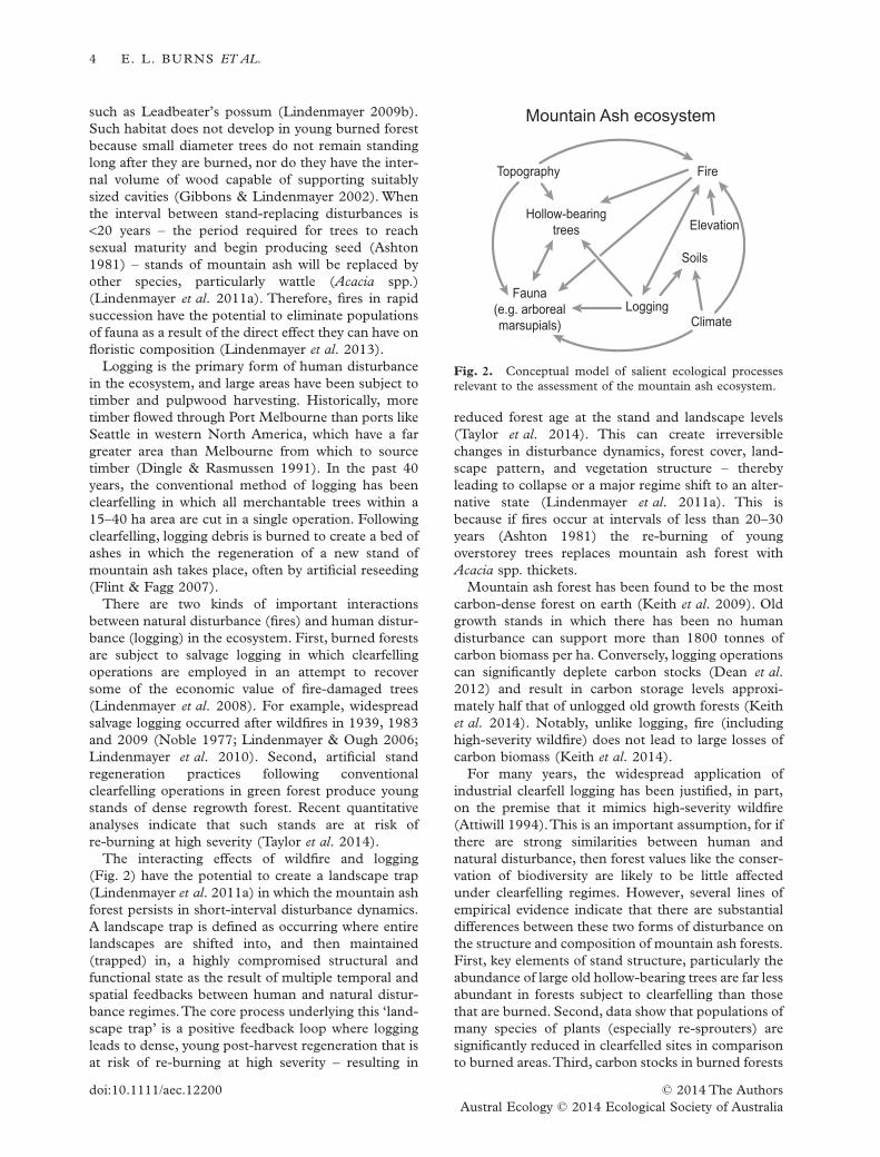
The interacting effects of wildfire and logging(Fig. 2) have the potential to create a landscape trap(Lindenmayer et al. 2011a) in which the mountain ashforest persists in short-interval disturbance dynamics.A landscape trap is defined as occurring where entirelandscapes are shifted into, and then maintained(trapped) in, a highly compromised structural andfunctional state as the result of multiple temporal andspatial feedbacks between human and natural distur-bance regimes.The core process underlying this ‘land-scape trap’ is a positive feedback loop where loggingleads to dense, young post-harvest regeneration that isat risk of re-burning at high severity – resulting in

reduced forest age at the stand and landscape levels(Taylor et al. 2014). This can create irreversiblechanges in disturbance dynamics, forest cover, land-scape pattern, and vegetation structure – therebyleading to collapse or a major regime shift to an alter-native state (Lindenmayer et al. 2011a). This isbecause if fires occur at intervals of less than 20–30years (Ashton 1981) the re-burning of youngoverstorey trees replaces mountain ash forest withAcacia spp. thickets.

Mountain ash forest has been found to be the mostcarbon-dense forest on earth (Keith et al. 2009). Oldgrowth stands in which there has been no humandisturbance can support more than 1800 tonnes ofcarbon biomass per ha. Conversely, logging operationscan significantly deplete carbon stocks (Dean et al.2012) and result in carbon storage levels approxi-mately half that of unlogged old growth forests (Keithet al. 2014). Notably, unlike logging, fire (includinghigh-severity wildfire) does not lead to large losses ofcarbon biomass (Keith et al. 2014).

For many years, the widespread application ofindustrial clearfell logging has been justified, in part,on the premise that it mimics high-severity wildfire(Attiwill 1994).This is an important assumption, for ifthere are strong similarities between human andnatural disturbance, then forest values like the conser-vation of biodiversity are likely to be little affectedunder clearfelling regimes. However, several lines ofempirical evidence indicate that there are substantialdifferences between these two forms of disturbance onthe structure and composition of mountain ash forests.First, key elements of stand structure, particularly theabundance of large old hollow-bearing trees are far lessabundant in forests subject to clearfelling than thosethat are burned. Second, data show that populations ofmany species of plants (especially re-sprouters) aresignificantly reduced in clearfelled sites in comparisonto burned areas.Third, carbon stocks in burned forests

Elevation

Climate

Soils

Topography

Mountain Ash ecosystem

Fire

Fauna(e.g. arborealmarsupials)

Hollow-bearingtrees

Logging

Fig. 2. Conceptual model of salient ecological processesrelevant to the assessment of the mountain ash ecosystem.



are depleted by 8–14% after fire but carbon stockreduction is up to five times greater in clearfelled areas(Keith et al. 2014). There are other major differencesbetween clearfelling and wildfire in mountain ashforests. Perhaps one of the most important is theoverall age structure of the forest. Under a rotation of50–80 years on cut sites, the mean age of the forest issignificantly younger than the overall mean age of aforest estate subject only to wildfire (McCarthy &Burgman 1995). Perhaps most critical now is the reali-zation that mountain ash forests are not subject toeither clearfell logging or fire, but rather both kinds ofdisturbance.That is, large parts of mountain ash foresthave experienced not only fire or clearfelling, but acombination of both in rapid succession (viz. salvagelogging). Some elements of the biota like Leadbeater’spossum are highly sensitive to all three kinds of distur-bance – fire, clearfelling and salvage logging. They arealso sensitive to the substantial changes to landscapesassociated with these disturbances, such as the wide-spread diminution of old growth cover. Finally, there isan increasing realization that human disturbance andnatural disturbance are not necessarily independentprocesses, as logged forests can be more prone to highseverity fire for prolonged (decadal) periods (Tayloret al. 2014).

METHODS

A comprehensive account of our interpretation and applica-tion of the IUCN Red List of Ecosystems criteria is providedat Appendix S2, which also provides details on the datasetsnamed below, and a more thorough explanation of ourapproach. Here we provide a brief overview.

Criterion A (decline in distribution)

This criterion requires an assessment of the amount ofchange in spatial distribution for each of the three timeperiods. (A1) A current decline ≥80% equates to a categoryof Critically Endangered (CR); ≥50% equates to Endangered(EN), and ≥30% equates toVulnerable (VU). If these are notmet, then a category of LC applies. (A2) The same levelsrelate to future decline. (A3) For historic decline ≥90%equates to a category of CR; ≥70% equates to EN and ≥50%equates to VU.

A1. Current decline: the decline in distribution over thepast 50 years (i.e. since 1964)

An assessment of the amount of change in spatial distribu-tion over the past 50 years is required.We first estimated thecurrent distribution (i.e. in 2014) of the mountain ash forestby interrogating three Victorian Government spatial layers:(i) the Statewide Forest Resource Inventory dataset; (ii) theLogging History dataset; and (iii) the Ecological VegetationClasses dataset. We then examined the Victorian Govern-ment’s Forest Management Zone dataset to determine theproportion of the ecosystem which occurred on public land.

We made our determination based on this proportion, and areview of the literature.

A2. Future decline: the predicted decline in spatialdistribution over the next 50 years (i.e. to 2064)

Similar to A1, we predicted future geographic distribution (in2064) based on land tenure. This was a highly conservativeapproach as we did not consider areas planned to be loggedunder the Timber Release Plan (Government of Victoria2011).The was primarily because these areas regenerate afterlogging and are therefore arguably still part of the geographicdistribution, albeit in a modified condition.

A3. Historical decline (sub-criterion 3): the decline inspatial distribution since 1750

Our estimate of decline here needed to differ from A1because the mapped classes employed in A1 were not avail-able from 1750. We therefore used the Australian Govern-ment dataset ‘NVIS Major Vegetation Subgroups’ whichprovided modelled vegetation cover pre-1750.

Criterion B (restricted geographic distribution)

Criterion B addresses (i) extent of occurrence; (ii) area ofoccupancy; and (iii) the number of ‘locations’ occupied rela-tive to the most serious plausible threat (where the number oflocations within an ecosystem is greater than 1, if the impactof threats will affect spatially discrete areas within the eco-system differently).

(i) To quantify the extent of occurrence, we created aminimum convex polygon that encompassed mapped distri-bution of the mountain ash ecosystem. (ii) Area of occupancywas based on 10 km2 grid cells. (iii) The number of locationswas based on wildfire as we consider this to be the mostextensive, unpredictable threat of varying severity. Weobtained information on the time and location of historicalfires from the Victorian Government dataset ‘FIRE100_YEAR’. To check the accuracy, we then overlayed themapping for the most extensive fire with our long-term fieldsites distributed throughout the Central Highlands of Victo-ria (see Lindenmayer et al. 2012).

Assessment for Criterion C, D and E

Three key concepts underpinned assessments for Criteria C,D and E: (i) ecosystem collapse; (ii) environmental degrada-tion; and (iii) relative severity (see Appendix S2 for anexplanation). For Criteria C and D, we evaluated degrada-tion of the abiotic environment and disruption to bioticprocesses and interactions, respectively. We did this by esti-mating the relative extent and severity of declines in therelevant variables.The severity estimates were assumed to bean average across 100% of the extent of the ecosystem.Therefore, only relative extent thresholds were used to dif-ferentiate between the three categories of threat: CR, EN andVU. For Criterion C1, C2, D1 and D2 the thresholds wereCR ≥ 80%, EN ≥ 50% andVU ≥ 30%. For Criterion C3 andD3 they were CR ≥ 90%, EN ≥ 70% andVU ≥ 50%.Variousother comparisons are possible when severity estimates do



not apply to 100% of the extent (see Table 1 of AppendixS2).

Collapse thresholds

Ecosystem collapse was considered to have occurred when:(i) 100% of the area where the ecosystem currently occurs

was no longer bioclimatically suitable (see Criterion Cmethods below). The climatic envelope range limitsdefined by the profile of the current distribution areshown Appendix S2. These thresholds were employedfor Criterion C2 analyses.

Or(ii) The abundance of hollow-bearing trees dropped below

1 per hectare averaged across the entire mountain ashecosystem. This threshold was employed for sub-criterion D2, and Criterion E analyses.

Or(iii) There was less than 1% of old-growth forest remaining

in the ecosystem. This threshold was employed forsub-criterion D1 and D3.

Our three forms of ecosystem collapse were defined asecosystem-wide averages. Therefore our assignment to riskcategories was dependent on the relative severity percentagesonly.

Criterion C

Criterion C entails an assessment of the ecosystem inresponse to the most important abiotic variable over threetime periods – since 1750 (C3), the past 50 years (since1964; C1), and in the future (until 2064; C2). Temperatureand precipitation and other climate-related variables wereused for Criterion C.

Criterion D

Criterion D requires an assessment for the same three timeperiods but in response to hollow-bearing trees, the principalbiotic variable. For Criterion D we drew on long-term fieldsurvey data, fire-history records and mapped old-growthforest. For D2, we investigated 39 scenarios based on varyingharvesting and fire regimes. To investigate the impact ofuncertainty in our definition of collapse, we varied the pointof collapse from 0.5 to 1.5 tree-hollows per ha at 0.1intervals.

Criterion E

Criterion E is an overarching analysis of the impacts of bioticvariables on the probability of ecosystem collapse within50–100 years. We ran simulations to investigate the futureresource of hollow-bearing trees by systematically exploringscenarios that differed in harvesting and fire regime and thedensity level of hollow-bearing trees that defined ecosystemcollapse.

We ran 10 000 stochastic simulations for 39 scenarios (thesame scenarios as used for D2). Each simulation consisted ofa random draw from the appropriate distribution for eachparameter.We then projected the results forward in the samemanner as for criterion D2. That is, we have 10 000 projec-

tions for each of the 39 scenarios which we then used tocalculate the probability of collapse.

Similar to D2, to investigate the sensitivity of the probabil-ity of collapse, we varied the definition of collapse for thenumber of hollow-bearing trees per ha. Additionally, we com-puted several percentiles of the simulations for each of the 39scenarios, which we present graphically and in tabular formin Appendix S4. The 10th, 20th and 50th percentiles of thesimulations gave an estimate of what number of hollowbearing trees per hectare we would have to set as a definitionof collapse, to result in a different endangerment category(i.e. VU vs. EN vs. CR respectively). We present a graphicalsummary of the 2.5th, the 50th and the 97.5th percentiles foreach of the 39 scenarios in Appendix S4.

RESULTS

The mountain ash forest is among one of the beststudied Australian ecosystems. Despite this, two of thesub-criteria were Data Deficient (DD) (Table 1).Overall, our allocated rankings ranged from LC to CRthereby leading to an overall risk category of CRbecause, as per the Keith et al. (2013) protocol, thehighest level of risk determines the final overall rating.

Criterion A – decline in distribution

A1. current decline (sub-criterion 1): the decline indistribution over the past 50 years (i.e. since 1964)

We estimated the current distribution of the mountainash ecosystem to be 156 700 ha, 96.4% of which is onpublic land. We assumed, due to stable land tenure(see below), that there had been virtually no change indistribution since 1964. The status of the mountainash ecosystem is therefore LC.

Approximately 20% of the mountain ash forestoccurs in closed water catchments, parts of which arealso managed as theYarra Ranges National Park. Areasof forest were closed for water supply purposes startingin the 1890s with several closed catchments addedprogressively after that time (Viggers et al. 2013). Theremaining 80% of mountain ash forest is located inareas broadly designated for paper pulp and timberproduction (Flint & Fagg 2007; Lindenmayer 2009a).Agreements regarding logging practices between watercatchment management authorities and the (then)Forests Commission of Victoria for the Central High-lands pre-date 1928 (Viggers et al. 2013).

A2. future decline (sub-criterion 2): the predicted declinein spatial distribution over the next 50 years(i.e. to 2064)

Almost the entire mountain ash forest occurs onpublic land.We therefore assumed that the distribution



would remain largely unchanged from 2014 until2064. The status of the ecosystem is therefore LC.

A3. historical decline (sub-criterion 3): the decline inspatial distribution since 1750

The amount of wet sclerophyll forest dominated bymountain ash has decreased from a modelled pre-1750 area of 183 000 ha to an extant area of180 000 ha, a reduction of approximately 2% (seeFig. 3). The status of the ecosystem is therefore LC.

Criterion B – distribution size: extent ofoccurrence and area of occupancy

B1 – extent of occurrence

The area of the minimum convex polygon enclosing allmapped occurrences (see Fig. 4) was 11 000 km2.However, before making a final determination under

Criterion B1 and B2, we assessed the number of loca-tions within the ecosystem (see Appendix S2). In1939, a single wildfire affected between approximately74% and 96% of the ecosystem. Our ‘best-estimate’ isthat 85% of the distribution of the ecosystem wasburnt (see Methods). This indicates that a singlethreatening event can affect almost the entire distribu-tion of the mountain ash ecosystem. Based on thisevidence, we concluded there are ≤2 locations withinthe ecosystem. The ecosystem is therefore EN. Weacknowledge that this approach does not account forregeneration following disturbances such as wildfire(Smith et al. 2013). However, the simplification of theecosystem through one such event is in itself sufficientto meet the endangered criterion for Criterion B1.

B2 – area of occupancy

We superimposed a 10 km2 grid over the mapped poly-gons of the mountain ash forest (see Fig. 4) and cal-culated that the ecosystem was present within 96 (of140) grid cells. Of these, 23 grid cells contained

Fig. 3. The estimated change in extent of the mountain ash ecosystem in the Central Highlands of Victoria since 1750.



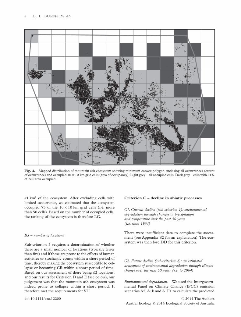
<1 km2 of the ecosystem. After excluding cells withlimited occurrence, we estimated that the ecosystemoccupied 73 of the 10 × 10 km grid cells (i.e. morethan 50 cells). Based on the number of occupied cells,the ranking of the ecosystem is therefore LC.

B3 – number of locations

Sub-criterion 3 requires a determination of whetherthere are a small number of locations (typically fewerthan five) and if these are prone to the effects of humanactivities or stochastic events within a short period oftime, thereby making the ecosystem susceptible to col-lapse or becoming CR within a short period of time.Based on our assessment of there being ≤2 locations,and our results for Criterion D and E (see below), ourjudgement was that the mountain ash ecosystem wasindeed prone to collapse within a short period. Ittherefore met the requirements for VU.

Criterion C – decline in abiotic processes

C1. Current decline (sub-criterion 1): environmentaldegradation through changes in precipitationand temperature over the past 50 years(i.e. since 1964)

There were insufficient data to complete the assess-ment (see Appendix S2 for an explanation). The eco-system was therefore DD for this criterion.

C2. Future decline (sub-criterion 2): an estimatedassessment of environmental degradation through climatechange over the next 50 years (i.e. to 2064)

Environmental degradation. We used the Intergovern-mental Panel on Climate Change (IPCC) emissionscenarios A2, A1b and A1F1 to calculate the predicted

Fig. 4. Mapped distribution of mountain ash ecosystem showing minimum convex polygon enclosing all occurrences (extentof occurrence) and occupied 10 × 10 km grid cells (area of occupancy). Light grey – all occupied cells. Dark grey – cells with ≥1%of cell area occupied.



losses of extent relative to climatic suitability underthese scenarios. From the current distribution of156 700 ha (see Table 2), the predicted losses at the50th percentile were 36 350 ha (23%), 29 900 ha(19%) and 70 500 ha (45%) respectively. Lowerbounds at the 10th percentile were 17%, 14% and47%, while upper bounds at the 90th percentile were97%, 98% and 100% respectively.

Relative severity. The amount of loss needed totrigger collapse is 156 700 ha; that is, the total currentextent of the mountain ash forest. Relative severityranged from 14% to 100%. This ranks the systembetween LC and CR (LC-CR).

Based on the 50th percentile predictions, and giventhat functional collapse will be realized prior to 100%physical loss of the ecosystem, we ranked the ecosys-tem as VU.

C3. Historical decline (sub-criterion 3): an assessment ofenvironmental degradation through changes inprecipitation and temperature since 1750

There were insufficient data to complete the assess-ment (see Methods and Appendix S2).The ecosystemwas therefore DD for this criterion.

Criterion D – decline in biotic processesand interactions

D1. Current decline (sub-criterion 1): environmentaldegradation resulting from the loss of hollow-bearing trees(using old-growth as a surrogate) over the past 50 years(i.e. since 1964)

Environmental degradation. There has been a signifi-cant reduction in the amount of old-growth since 1964(Table 2).We estimated that the area of mountain ashforest that was unlogged and unburnt by wildfire in1964 was 6300 ha (4% of the estate). This had beenreduced by 4600 ha (i.e. the observed decline) to1700 ha (1% of the estate) by 2011. Note that theestimate of 6300 ha was derived using the 1939 fireextent mapping layer which we considered to be anover-estimate by approximately 11%. Because wecannot determine the spatial interaction with loggingwhile accounting for this error, we do not providebounds on our estimate.

Relative severity. To trigger ecosystem collapse, theamount of old growth forest would need to decline to1400 ha (which equals 0.9% of 156 700 ha anapproximation for <1% old-growth forest remaining inthe current ecosystem; see Methods). Therefore, the

Table 2. Summary of mountain ash extent (hectares) logged or burnt by large wildfires

Threat

Last 50 years Since 1750 Next 50 years

All Old-Growth Mature All Old-Growth Mature All Old-Growth Mature

LoggingTotal logging 55 300 1000 42 300 >62 800 >1 000 >49 300 113 600 (unless

capped at83 750)

0 33 000 (unlesscapped at21 700)

Percentage 35% 0.6% 27% >40% >0.6% >32% 73%or 54% ifcapped

21%; or 14%if capped

Salvage logging 7 900 600 4 800 >7 900 >600 >4 800 Depends onfire regime

Depends onfire regime

Depends onfire regime

Percentage 5% 0.4% 3% >5% >0.4% >3%Large wildfires

1939 150 400* >45 100 unknown 80 400 1600 49 500Percentage 96%* >29% 51% 1% 32%

1983 17 250 1100 14 900 17 250 1 100 14 900 9 200 200 5 700Percentage 11% 0.7% 9.5% 11% 0.7% 9.5% 6% 0.1% 4%

2009 53 400 3100 35 350 53 400 3 100 35 350 28 500 600 17 500Percentage 34% 2% 23% 34% 2% 23% 18% 0.4% 11%

Estimated pre-1750 extent <183 000 ha (note this is based on wet sclerophyll forest that is predominantly mountain ash – see Appendix S2);Estimated pre-1964 extent = 156 700 ha; Estimated current extant = 156 700 ha; Old-growth defined as forest with no wildfire or logging sincerecords began (1903 for fire and 1932 for logging); Mature defined as 1939 regrowth; Note. Some areas of forest burnt in the wildfires were subjectto salvage logging (as estimated above) but we do not know how much was salvage logged after the 1939 fire.The estimates of area logged or burntare not necessarily mutually exclusive, but logged and burnt = salvage logging. *This value was derived as per the values shown in this Tablefor the 1983 and 2009 fires. However, see Methods and Appendix S2 for our revised estimate of 85% extent, which is approximately133 200 ha.



loss needed to achieve ecosystem collapse was:approximately 6300 ha (Total predicted area of oldgrowth in the absence of logging in 1964) − 1400(ecosystem collapse level) = 4900 ha, yielding a rela-tive severity of approximately 94% (i.e. 4600/4900 × 100). We concluded that the disruption ofbiotic processes over the past 50 years, based on achange in the number of hollow-bearing trees (usingold-growth as a surrogate), indicated a decline with≥80% relative severity (average across 100% extent;see Appendix S2). The ecosystem is therefore CR. Tochange this ranking would require a relative severityof less than 90%, requiring the 1964 area of oldgrowth to be <4400 ha (an error of 70%) which isimprobable.

D2. Future decline (sub-criterion 2): environmentaldegradation resulting from the projected loss ofhollow-bearing trees over the next 50 years

For projections of future decline in the abundance ofhollow-bearing trees, we utilized empirical researchdata from long-term field sites. We could not do thisfor the other two time periods because data collectionon the condition and abundance of hollow-bearingtrees commenced in 1997. Our projections includedprovision for ongoing clearfell logging underthe Victorian Government’s Timber Release Plan(Government of Victoria 2011) and future fires,both of which can accelerate the loss of large hollow-bearing trees in mountain ash ecosystems (see Appen-dix S2).

Our modelling projected a severe decline in theaverage number of large old hollow-bearing treesacross the mountain ash forest from approximately3.77 ha−1 in 2011 to approximately 0.29–0.82 ha−1 by2067 (Table 3, and Appendix S3 for full data). Thelower bound in the range of values was from the sce-nario based on simulating the occurrence of a firebefore 2067 that was equal in extent to the 1939 fire(1939 + 1983 re-growth harvesting scenario, largefire extent; see Appendix S2 and S3).The highest valuesin the range for the abundance of hollow-bearing treesresult from the scenario with no future fire or logging(Table 3, and Appendix S2). Therefore, our ‘observedestimate of decline’ in the best case scenario was 78%and the worst case scenario was 92% (Table 3).

We defined ecosystem collapse as occurring whenthe average abundance of hollow-bearing treesdeclined to <1 hollow-bearing tree per ha (see Appen-dix S2). Modelling in all 39 scenarios (3 harvestingscenarios by 13 fire regimes) projected a decline of≥78% with ≥100% relative severity (averaged across100% extent of the ecosystem) (see Appendix S3).Theecosystem is therefore CR, with plausible bounds alsowithin this category.

Interrogation of the sensitivity of the relative severityand ecosystem ranking to variation in the definition ofcollapse between 0.5 to 1.5 hollow-bearing trees perha showed that all relative severities remained above90% (see Table 3 and Appendix S3). This means thatthe ecosystem would remain ranked as CR under D2even if the definition of collapse was set at 0.5 hollow-bearing trees per ha (half what we consider to be theappropriate level).

Table 3. Projections of hollow bearing trees per hectare in 2067, change relative to 2011, relative severity and its sensitivity tovarying the definition of collapse (the number of hollow bearing trees per hectare) by fire/harvesting scenario

Harvestingscenario

Fireregime

2067 projected(hbt/ha)

Percentage declinefrom 2011

Relative severity, sensitivity

1.5 htb/ha 1.0 hbt/ha 0.5 hbt/ha

No harvesting No fire 0.82 78.36 130.1 106.7 90.3Small 0.77 79.62 146.3 108.4 91.8Medium 0.67 82.26 132.2 112.0 94.8Large 0.45 88.11 136.6 119.9 101.6

1939 + 1983 No fire 0.58 84.67 140.6 115.2 97.6Small 0.56 85.26 152.1 116.0 98.3Medium 0.48 87.23 141.6 118.7 100.6Large 0.32 91.56 144.9 124.6 105.6

1983 No fire 0.77 79.48 132.0 108.2 91.6Small 0.73 80.71 147.7 109.8 93.0Medium 0.63 83.27 134.0 113.3 96.0

We considered three different harvesting scenarios (no harvesting, 1983 regrowth only, and 1939 & 1983 regrowth), four fireregimes (no fire in the next 56 years and a small, medium and large fire extent).We report results for 2067, the final interval (theadditional intervals are given in the Appendix S3). We calculated the projected number of hollow bearing trees for each of theabove scenarios and computed the percentage decline in 2067 relative to 2011 and the relative severity using 1.5, 1.0 and 0.5hollow bearing tree per hectare as our definitions of collapse to investigate the sensitivity to varying the definition of collapse.Values >100% indicate collapse and replacement by a novel ecosystem with reduced diversity of vertebrate fauna and fewlarge trees.



D3. Historical decline (sub-criterion 3): an assessment ofenvironmental degradation and relative severity througha loss of hollow-bearing trees (using old-growth as asurrogate) since 1750

Environmental degradation. It is not known how muchold-growth forest was present within the mountain ashecosystem in 1750. However, Lindenmayer et al.(2014a) suggest that between 30–60% of the forestwas formerly old-growth. The current extent of themountain ash forest is 156 700 ha, of which aminimum of 47 000 ha (30%) is estimated to havebeen old-growth in 1750 (see Table 2). The currentarea of old-growth forest is 1700 ha. Therefore, ourlower bound ‘observed estimate of decline’ in theamount of old growth is 45 300 ha.

Relative severity. We defined ecosystem collapse forCriterion D as occurring when the area of old growthforest was <1400 ha (see Appendix S2). The level ofloss needed to trigger ecosystem collapse was: 47 000(Total pre-1750 old growth) – 1400 (ecosystem col-lapse level) = 45 600 ha, yielding a relative severity of99% (i.e. 45 300/45 600 * 100). We therefore con-cluded (based on the lower bound of the range in oldgrowth cover) that the disruption to biotic process overthe past 50 years has led to a decline with ≥90%relative severity. The ecosystem is therefore CR, withlower and upper plausible bounds within this ranking.

Criterion E – quantitative assessment of theprobability of ecosystem collapse within100 years

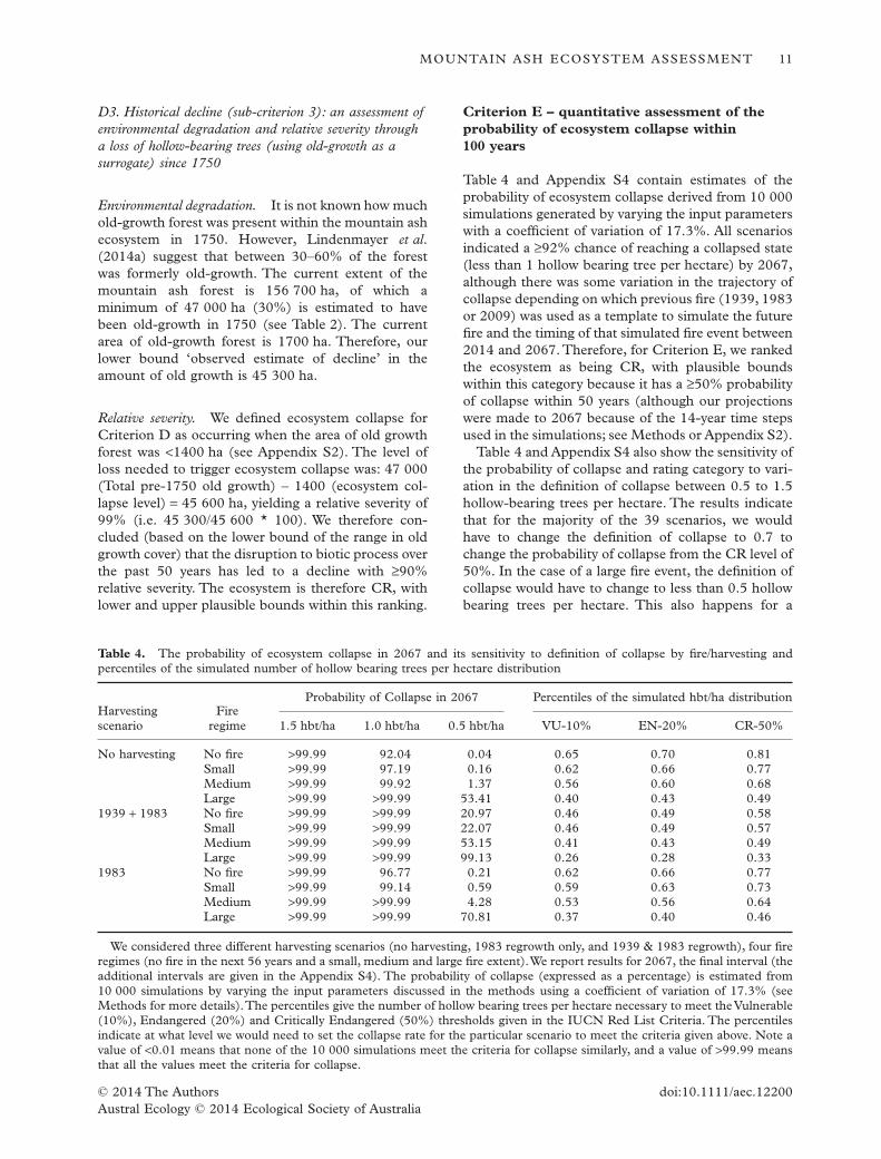
Table 4 and Appendix S4 contain estimates of theprobability of ecosystem collapse derived from 10 000simulations generated by varying the input parameterswith a coefficient of variation of 17.3%. All scenariosindicated a ≥92% chance of reaching a collapsed state(less than 1 hollow bearing tree per hectare) by 2067,although there was some variation in the trajectory ofcollapse depending on which previous fire (1939, 1983or 2009) was used as a template to simulate the futurefire and the timing of that simulated fire event between2014 and 2067.Therefore, for Criterion E, we rankedthe ecosystem as being CR, with plausible boundswithin this category because it has a ≥50% probabilityof collapse within 50 years (although our projectionswere made to 2067 because of the 14-year time stepsused in the simulations; see Methods or Appendix S2).

Table 4 and Appendix S4 also show the sensitivity ofthe probability of collapse and rating category to vari-ation in the definition of collapse between 0.5 to 1.5hollow-bearing trees per hectare. The results indicatethat for the majority of the 39 scenarios, we wouldhave to change the definition of collapse to 0.7 tochange the probability of collapse from the CR level of50%. In the case of a large fire event, the definition ofcollapse would have to change to less than 0.5 hollowbearing trees per hectare. This also happens for a

Table 4. The probability of ecosystem collapse in 2067 and its sensitivity to definition of collapse by fire/harvesting andpercentiles of the simulated number of hollow bearing trees per hectare distribution

Harvestingscenario

Fireregime

Probability of Collapse in 2067 Percentiles of the simulated hbt/ha distribution

1.5 hbt/ha 1.0 hbt/ha 0.5 hbt/ha VU-10% EN-20% CR-50%

No harvesting No fire >99.99 92.04 0.04 0.65 0.70 0.81Small >99.99 97.19 0.16 0.62 0.66 0.77Medium >99.99 99.92 1.37 0.56 0.60 0.68Large >99.99 >99.99 53.41 0.40 0.43 0.49

1939 + 1983 No fire >99.99 >99.99 20.97 0.46 0.49 0.58Small >99.99 >99.99 22.07 0.46 0.49 0.57Medium >99.99 >99.99 53.15 0.41 0.43 0.49Large >99.99 >99.99 99.13 0.26 0.28 0.33

1983 No fire >99.99 96.77 0.21 0.62 0.66 0.77Small >99.99 99.14 0.59 0.59 0.63 0.73Medium >99.99 >99.99 4.28 0.53 0.56 0.64Large >99.99 >99.99 70.81 0.37 0.40 0.46

We considered three different harvesting scenarios (no harvesting, 1983 regrowth only, and 1939 & 1983 regrowth), four fireregimes (no fire in the next 56 years and a small, medium and large fire extent).We report results for 2067, the final interval (theadditional intervals are given in the Appendix S4). The probability of collapse (expressed as a percentage) is estimated from10 000 simulations by varying the input parameters discussed in the methods using a coefficient of variation of 17.3% (seeMethods for more details).The percentiles give the number of hollow bearing trees per hectare necessary to meet theVulnerable(10%), Endangered (20%) and Critically Endangered (50%) thresholds given in the IUCN Red List Criteria. The percentilesindicate at what level we would need to set the collapse rate for the particular scenario to meet the criteria given above. Note avalue of <0.01 means that none of the 10 000 simulations meet the criteria for collapse similarly, and a value of >99.99 meansthat all the values meet the criteria for collapse.



scenario characterized by a fire of medium spatialextent and current logging practice, that is, loggingboth 1939 and 1983 regrowth stands.

DISCUSSION

We have used the protocol developed by Keith et al.(2013) to complete a detailed assessment of the moun-tain ash forest ecosystem. A notable outcome of ourinvestigation was that we identified markedly differentestimates of risk – ranging from LC through to CR –depending on which aspects of the ecosystem wereunder consideration. For example, the distribution ofthe ecosystem (Criterion A) has undergone remark-ably little reduction over the past 50 years and wasclassified as LC. However, examination of the disrup-tion to the biotic process of hollow-bearing trees forCriterion D showed the ecosystem to be CR for alltime periods examined. This is because of a positivefeedback between logging and fire (Lindenmayer et al.2011b; Taylor et al. 2014) which significantly impairsthe recruitment of large old trees and old growth forestin the mountain ash ecosystem (Lindenmayer et al.2012, 2014a). Under Criterion E, interactions such asthese can be explicitly assessed through stochasticmodelling. Ideally, for Criterion E, in our stochasticmodel which predicts the probability of ecosystem col-lapse within 50 to 100 years, we would also haveincorporated the various climate change scenariosconsidered under Criterion C. However, we did nothave sufficient data to compute collapse rates ofhollow-bearing trees under the various climate changeregimes. We therefore utilized only available data onthe decline of hollow-bearing trees (see Criterion D)to complete the assessment. Nevertheless, our model-ling highlighted the risk of collapse of the ecosystemwithin a very short time. The rank of CR under Cri-terion E is a result of the rapidly declining abundanceof large old hollow-bearing trees and the limitedcurrent area of old growth forest in the ecosystem.

Although there were marked differences in the assess-ment outcome,depending on which criterion was beingexamined (seeTable 1),we suggest that this is a strengthand not a weakness of the approach. Indeed, we arguethere is considerable merit in an ecosystem assessmentprocess that is underpinned by a range of criteria.Thisis because a single metric may not provide a detailedpicture of the status of a given ecosystem. This washighlighted in our case study in which current area ofoccupancy had changed little relative to historicalextent, but major changes in biotic variables suggestedthat the ecosystem is at high risk of collapse within thenext 50 years (Table 4).The lack of ranking among thedifferent criteria allows a level of flexibility or pragma-tism within the assessment framework.This is becausedifferent ecosystems will be DD in different respectsand this should not unduly influence the overall rating.

This does, however, raise interesting questions as towhether a minimum set of criteria should be addressedand, if so, which criteria should comprise this minimumset? However, prescribing such an approach mightgenerate perverse outcomes rather than introduceincreased robustness, and we would want to examinemultiple systems and determine the effects of differentcombinations of criteria before advocating any givenapproach that ranks certain criteria over others.

The application of the protocol developed by Keithet al. (2013) provided a platform on which to assemblecurrent knowledge of the status of, and threats to, themountain ash forest. It also helped identify key knowl-edge gaps such as: (i) the paucity of data on pre-1939logging operations and post-fire salvage harvesting,both of which are likely to have had profound impactson the ecosystem (Lindenmayer 2009a); and (ii) thelack of long-term climatic data for the study region,which led to two categories of Criterion C beingranked as DD (see Appendix S2). However, we alsofound that the protocol was difficult to use because themountain ash ecosystem is so well understood as aresult of several decades of intensive research.That is,the availability of data on the ecosystem meant thatthere were difficult choices to be made about whichsub-criteria within particular criterion, and which vari-ables, were the most suitable for the purposes of theassessment (e.g. for Criterion B).The selection of dif-ferent options within sub-criterion B2 may have led todifferent outcomes for categories of threat. We there-fore suggest an important future step will be to com-plete a sensitivity analysis to determine the robustnessof assessment outcomes to the different optionschosen for assessment. In part, we tried to include thisin our approach (see Table 3 and 4) by examining thesensitivity of our informed ‘choice’ of collapse being 1hollow-bearing tree per hectare, and by taking an alter-native perspective and asking:What would the numberof hollow-bearing trees per hectare need to be to alterour risk assessment from CR under Criterion E? Wewould encourage the incorporation of these types ofanalyses in other applications of the criterion in differ-ent ecosystems in the future. Sensitivity analyses arealso common in other kinds of risk assessmentapproaches like Population Viability Analysis (PVA).Like the IUCN Criteria, PVA can be data intensiveand complex in nature. PVA has been used in the pastwithin the mountain ash ecosystem, but primarily toexplore the impacts of fire, logging, managementactions and other drivers on the possible persistence ofpopulations of various individual species of arborealmarsupials (e.g. Lindenmayer & Lacy 1995;Lindenmayer & Possingham 1996; Lindenmayer &McCarthy 2006).We did not use PVA here because wedid not focus on individual populations within theecosystem, but it would be interesting to compare theoutcomes of a series of PVAs of specific populations



within the ecosystem, which are dependent on theprocesses examined here. Similar to Criterion E, PVAsgenerate predictions of the relative risk of extinction interms of a probability of extinction or quasi-extinction(Possingham et al. 2013). But unlike the IUCN Crite-ria, PVAs are not employed at an ecosystem level, andestimates are not bounded within pre-defined timeperiods. Both approaches have their utility but theIUCN Criteria is a single application that can examinemany processes relevant to multiple populationswithin an ecosystem. A focus on key ecosystem pro-cesses can help improve understanding of other envi-ronments where similar kinds of processes may beimportant. As an example, understanding of the com-bined effects of fire and logging in the mountain ashforest has general lessons for other logged tall wetforested ecosystems. Similarly, the disruption of age-classes and how this undermines an ecosystem’s abilityto support hollow-bearing trees has general applicabil-ity to other ecosystems such as temperate eucalyptwoodlands which also support populations of cavity-dependent arboreal marsupials and birds.

We provide discussion on the management implica-tions of our assessment in Appendix S5.

ACKNOWLEDGEMENTS

We thank David Keith for his reviews of the manu-script prior to submission. We also thank two anony-mous reviewers whose comments led to an improvedmanuscript. Our ongoing work in the mountain ashecosystem is part of the Long Term EcologicalResearch Network (LTERN) which is part of the Ter-restrial Ecosystem Research Network (TERN). Othersupport funding for the plot network in Victorianmountain ash forests comes from the AustralianResearch Council, the Victorian Department ofPrimary Industries, Parks Victoria and Fujitsu Labo-ratories Limited. We acknowledge the following mod-elling groups: the Program for Climate ModelDiagnosis and Intercomparison (PCMDI), and theWCRP’s Working Group on Coupled Modelling(WGCM) for their roles in making available theWCRP CMIP3 multi-model dataset. Support of thisdataset is provided by the Office of Science, U.S.Department of Energy.

REFERENCES

Ashton D. H. (1975) The seasonal growth of Eucalyptus regnansF. Muell. Aust. J. Bot. 23, 239–52.

Ashton D. H. (1981) Tall open forests. In: Australian Vegetation(ed. R. H. Groves) pp. 121–51. Cambridge University Press,Cambridge.

Attiwill P. M. (1994) Ecological disturbance and the conserva-tive management of eucalypt forests in Australia. For. Ecol.Manage. 63, 301–46.

Beale R. (2007) If Trees Could Speak. Stories of Australia’s GreatestTrees. Allen and Unwin, Sydney.

Boitani L., Mace G. M. & Rondinini C. (2014) Challenging thescientific foundations for an IUCN Red List of Ecosystems.Conserv. Lett. doi: 10.1111/conl.12111

Boland D. J., Brooker M. I., Chippendale G. M. et al. (2006)Forest Trees of Australia. CSIRO Publishing, Melbourne.

Campbell R. G. (1984) The eucalypt forests. In: Silvicultural andEnvironmental Aspects of Harvesting Some Major CommercialEucalypt Forests inVictoria:A Review (eds R. G. Campbell, E.A. Chesterfield, F. G. Craig et al.) pp. 1–12. Forests Com-mission Victoria, Melbourne.

Dean C., Wardell-Johnson G. W. & Kirkpatrick J. B. (2012) Arethere any circumstances in which logging primary wet-eucalypt forest will not add to the global carbon burden?Agric. For. Meteorol. 161, 156–69.

Department of the Environment and Water Resources (2007)Australia’s NativeVegetation: A Summary of Australia’s MajorVegetation Groups. Australian Government, Canberra.

Dingle T. & Rasmussen C. (1991) Vital Connections: Melbourneand its Board ofWorks. Penguin Books, Melbourne, pp. 1891–991.

Flint A. & Fagg P. (2007) Mountain ash in Victoria’s StateForests. Department of Sustainability and Environment,Melbourne.

Florence R. G. (1996) Ecology and Silviculture of Eucalypt Forests.CSIRO Publishing, Melbourne.

Gibbons P. & Lindenmayer D. B. (2002) Tree Hollows andWildlife Conservation in Australia. CSIRO Publishing,Melbourne.

Government of Victoria (2011) Timber Release Plan 2011–2016.VicForests, Melbourne.

IUCN (2001) IUCN Red List Categories and Criteria:Version 3.1.IUCN Species Survival Commission, Gland.

Keith D. A., Rodríguez J. P., Rodríguez-Clark K. M. et al. (2013)Scientific foundations for an IUCN Red List of Ecosystems.PLoS ONE 8, e62111.

Keith H., Lindenmayer D. B., Mackey B. G. et al. (2014) Man-aging temperate forests for carbon storage: impacts oflogging versus forest protection on carbon stocks. Ecosphere5, Art. 75. Available from URL: http://dx.doi.org/10.1890/ES1814-00051.00051

Keith H., Mackey B. G. & Lindenmayer D. B. (2009)Re-evaluation of forest biomass carbon stocks and lessonsfrom the world’s most carbon-dense forests. Proc. Natl Acad.Sci. USA 106, 11635–40.

Lindenmayer D. B. (2009a) Forest Pattern and Ecological Process:A Synthesis of 25 Years of Research. CSIRO Publishing,Melbourne.

Lindenmayer D. B. (2009b) Old forests, new perspectives:insights from the mountain ash forests of the Central High-lands of Victoria, south-eastern Australia. For. Ecol. Manage.258, 357–65.

Lindenmayer D. B., Blair D., McBurney L. & Banks S. (2010)Forest Phoenix. How a Great Forest Recovers After Wildfire.CSIRO Publishing, Melbourne.

Lindenmayer D. B., Blair D., McBurney L. et al. (2014a) Prin-ciples and practices for biodiversity conservation and resto-ration forestry: a 30 year case study on the Victorianmontane ash forests and the critically endangeredLeadbeater’s Possum. Aust. Zoolog. 36, 441–60.

Lindenmayer D. B., Blanchard W., McBurney L. et al. (2012)Interacting factors driving a major loss of large treeswith cavities in a forest ecosystem. PLoS ONE 7,e41864.



http://dx.doi.org/10.1890/ES1814-00051.00051

http://dx.doi.org/10.1890/ES1814-00051.00051

Lindenmayer D. B., Blanchard W., McBurney L. et al. (2013)Fire severity and landscape context effects on arborealmarsupials. Biol. Conserv. 167, 137–48.

Lindenmayer D. B., Blanchard W., McBurney L. et al. (2014b)Complex responses of birds to landscape-level fire extent,fire severity and environmental drivers. Divers. Distrib. 20,467–77.

Lindenmayer D. B., Burton P. J. & Franklin J. F. (2008) SalvageLogging and Its Ecological Consequences. Island Press, Wash-ington DC.

Lindenmayer D. B., Cunningham R. B., Donnelly C. F., TantonM.T. & Nix H. A. (1993) The abundance and developmentof cavities in Eucalyptus trees: a case-study in the montaneforests ofVictoria, southeastern Australia. For. Ecol. Manage.60, 77–104.

Lindenmayer D. B., Hobbs R. J., Likens G. E., Krebs C. & BanksS. C. (2011a) Newly discovered landscape traps produceregime shifts in wet forests. Proc. Natl Acad. Sci. USA 108,15887–91.

Lindenmayer D. B. & Lacy R. C. (1995) Metapopulationviability of arboreal marsupials in fragmented old-growthforests: comparison among species. Ecol. Appl. 5, 183–99.

Lindenmayer D. B. & McCarthy M. A. (2006) Evaluation ofPVA models of arboreal marsupials: coupling models withlong-term monitoring data. Biodivers. Conserv. 15, 4079–96.

Lindenmayer D. B., Mackey B. G., Mullen I. C. et al. (1999)Factors affecting stand structure in forests – are there cli-matic and topographic determinants? For. Ecol. Manage.123, 55–63.

Lindenmayer D. B., Mackey B. G. & Nix H. A. (1996) Thebioclimatic domains of four species of commercially impor-tant eucalypts from south-eastern Australia. Aust. For. 59,74–89.

Lindenmayer D. B. & Ough K. (2006) Salvage logging in themontane ash eucalypt forests of the Central Highlands ofVictoria and its potential impacts on biodiversity. Conserv.Biol. 20, 1005–15.

Lindenmayer D. B. & Possingham H. P. (1996) Ranking conser-vation and timber management options for Leadbeater’sPossum in southeastern Australia using Population ViabilityAnalysis. Conserv. Biol. 10, 235–51.

Lindenmayer D. B., Wood J., McBurney L. et al. (2011b) Cross-sectional versus longitudinal research: a case study of treeswith hollows and marsupials in Australian forests. Ecol.Monogr. 81, 557–80.

Lumsden L. F., Alexander J. S. A., Hill F. A. R., Krasna S. P. &Silveira C. E. (1991) The Vertebrate Fauna of the Land Con-servation Council Melbourne-2 study area. Arthur Rylah Insti-tute for Environmental Research, Melbourne.

McCarthy M. A. & Burgman M. A. (1995) Coping with uncer-tainty in forest wildlife planning. For. Ecol. Manage. 74,23–36.

McCarthy M. A. & Lindenmayer D. B. (1998) Multi-agedmountain ash forest, wildlife conservation and timberharvesting. For. Ecol. Manage. 104, 43–56.

Mackey B., Lindenmayer D. B., Gill A. M., McCarthy M. A. &Lindesay J. A. (2002) Wildlife, Fire and Future Climate:A Forest Ecosystem Analysis. CSIRO Publishing, Melbourne.

McKenzie N. J., Isbell R. F., Jacquier D. W. & Brown K. L.(2004) Australian Soils and Landscapes: An IllustratedCompendium. CSIRO Publishing, Melbourne.

Mueck S. G. (1990) The floristic composition of mountain ash andAlpine Ash forests in Victoria. Department of Conservationand Environment, Melbourne.

Nicholson E., Regan T. J., Auld T. D. et al. (2014) Towardsconsistency, rigour and compatibility of risk assessments forecosystems and ecological communities. Austral Ecol. doi:10.1111/aec.12148

Nitschke C. & Hickey G. (2007) Assessing the Vulnerabilityof Victoria’s Central Highlands Forests to ClimateChange. Department of Sustainability and Environment,Melbourne.

Noble W. S. (1977) Ordeal by Fire.TheWeek a State Burned Up.Hawthorn Press, Melbourne.

Possingham H. P., Lindenmayer D. B. & McCarthy M. A. (2013)Population viability analysis. In: Encyclopedia of Biodiversity(ed. S. A. Levin) pp. 210–219. Elsevier, Amsterdam.

Rodríguez J. P., Rodríguez-Clark K. M., Baillie J. E. M. et al.(2011) Establishing IUCN Red List Criteria for threatenedecosystems. Conserv. Biol. 25, 21–9.

Smith A. L., Blair D., McBurney L. et al. (2013) Dominantdrivers of seedling establishment in a fire-dependent obli-gate seeder: climate or fire regimes? Ecosystems 17, 258–70.

Taylor C., McCarthy M. A. & Lindenmayer D. B. (2014) Non-linear effects of stand age on fire severity. Conserv. Lett. 7,355–70.

Viggers J. I., Weaver H. J. & Lindenmayer D. B. (2013) Mel-bourne’s Water Catchments: Perspectives on a World Class WaterSupply. CSIRO Publishing, Melbourne.

Wood S., Bowman D., Prior L., Lindenmayer D. B., Wardlaw T.& Robinson R. (2014) Tall eucalypt forests. In: Biodiversityand Environmental Change: Monitoring, Challenges and Direc-tion (eds D. B. Lindenmayer, E. Burns, N. Thurgate & A.Lowe) pp. 519–69. CSIRO Publishing, Melbourne.

Xu T. & Hutchinson M. F. (2013) New developments andapplications in the ANUCLIM spatial climatic and biocli-

matic modelling package. Environ.Model.Softw. 40, 267–79.

SUPPORTING INFORMATION

Additional Supporting Information may be found inthe online version of this article at the publisher’sweb-site:

Appendix S1. Information on flora and fauna in themountain ash ecosystem.Appendix S2. Detailed Methods for the EcosystemAssessment.Appendix S3. Results – Supplementary material forCriterion D2: Projections of hollow bearing trees perhectare in 2067 by fire/harvesting scenario; and Sen-sitivity of relative severity to changing the definition ofcollapse by fire/harvesting scenario.Appendix S4. Results – Supplementary material forCriterion E: Probability of collapse by fire/harvestingscenario, tree hollow/hectare density, and year; andSensitivity of the probability of collapse to varying thedefinition of collapse by fire/harvesting scenario.Appendix S5. Management Implications – Supple-mentary material for the Discussion.



ecosystem assessment of mountain ash forest in the … · ecosystem assessment of mountain ash...

Documents