ecosystem goods and services in production landscapes in

Ecosystem Goods and Services in Production

Landscapes in South-Eastern Australia

By

Himlal Baral

MA, MSc

Submitted in total fulfillment of the requirements of the degree of

Doctor of Philosophy

October 2013

Department of Forest and Ecosystem Science

Melbourne School of Land and Environment

The University of Melbourne

i

ABSTRACT

Ecosystem goods and services (EGS), the benefits that humans obtain from ecosystems, are vital for

human well-being. As human populations increase so do demands for almost all EGS. Managing

changing landscapes for multiple EGS is therefore a key challenge for resource planners and decision

makers. However, in many cases the supply of different types of goods and services can conflict. For

example, the enhancement of provisioning services can lead to declines in regulating and cultural

services, but there are few tools available for analysing these trade-offs in a spatially-explicit way.

This thesis developed approaches and tools for spatially explicit measurement and management of

multiple EGS provided by production landscapes. These were used to assess the impacts of land-use

change and to provide a basis for managing these trade-offs using case studies in two contrasting

production landscapes in south-eastern Australia. Both landscapes have been subject to extensive

clearing of native vegetation, which is now present in remnant patches. One study landscape had a

concentration of commercially-valuable hardwood and softwood plantations, and the other was

dominated by land traditionally focused on agricultural production that is currently being re-

configured to provide for more sustainable farming practices and to increase provision of multiple

ecosystem services.

The study involved five components: (i) development of a novel, qualitative approach for rapid

assessment of EGS in changing landscapes that was used to assess observed and potential changes in

land use and land cover and their impact on the production of different EGS (Chapter 2); (ii)

development and testing of an approach for assessing multiple EGS across space and time using a

case study of six key EGS in a sub-catchment in Lower Glenelg Basin, south-western Victoria that

demonstrated landscape-scale trade-offs between provisioning and many regulating services (Chapter

3); (iii) an economic valuation of EGS using market and non-market techniques to produce spatial

economic value maps (Chapter 4); (iv) spatial assessment of the biodiversity values that underpin

provision of many ecosystem services utilising a variety of readily available data and tools (Chapter

5); and (v) assessment of trade-offs and synergies among multiple EGS under current land use and

realistic future land-use scenarios (Chapter 6).

Results indicate that EGS can be assessed and mapped in a variety of ways depending on the

availability of data, time, and funding as well as level of detail and accuracy required. A qualitative

assessment can be useful for an initial investigation (Chapter 2) while quantitative and monetary

assessments may be required for detailed landscape-scale planning (Chapters 3, 4). In addition, the

provision of EGS by production landscapes can vary considerably depending on land use and land

cover, and management choices. The study demonstrates that landscapes dedicated mostly to

ii

agricultural production have limited capacity to produce the range of ecosystem services required for

human health and well-being, while landscapes with a mosaic of land uses can produce a wide range

of services, although these are often subject to trade-offs between multiple EGS (Chapters 2, 3).

Furthermore, the study demonstrated that spatial assessment and mapping of biodiversity value plays

a vital role in identifying key areas for conservation and establishing conservation priorities to

allocate limited resources (Chapter 5). There is potential for an improved balance of the multiple EGS

required for human health and well-being at the landscape scale, although the economic incentive to

adopt more sustainable land use practices that produce a wide range of services are compromised due

to the lack of economic valuation of public ecosystem services (Chapter 6). High hopes have been

placed by researchers on spatial assessment, mapping and economic valuations of ecosystem goods

and services to influence policy makers for coping with the accelerating degradation of natural capital.

The approaches and tools used in this thesis can potentially enhance our collective choices regarding

the management of landscapes for multiple values and can help policy makers and land managers to

enhance the total benefits that landscapes provide to societies through the provision of an optimal mix

of goods and services.

iii

DECLARATION

This is to certify that:

i. The thesis comprises only my original work.

ii. Due acknowledgement has been made in the text to all other material used.

iii. The thesis is less than 100,000 words in length, exclusive of tables, illustrations, bibliography,

and appendices.

... ... ... ... ... ...

Himlal Baral

1 October 2013

iv

PREFACE

This PhD thesis consists of seven chapters four of which have been published. I conducted the

majority of research work for these publications while the co-authors contributed in the form of

overall supervision from site selection, stakeholder consultation, resource supply and editorial support

on manuscript writing. The citations for the published chapters and those in review are as follows:

Chapter 2

Baral, H., Keenan, R.J., Stork, N.E., Kasel, S., 2013. Measuring and managing ecosystem goods and

services in changing landscapes: a south-east Australian perspective. Journal of Environmental

Planning and Management (in press) http://dx.doi.org/10.1080/09640568.2013.824872

Chapter 3

Baral, H., Keenan, R.J., Fox, J.C., Stork, N.E., Kasel, S., 2013. Spatial assessment of ecosystem

goods and services in complex production landscapes: A case study from south-eastern Australia.

Ecological Complexity 13, 35–45.

Chapter 4

Baral, H., Kasel, S., Keenan, R. J., Fox, J., Stork, N., 2009. GIS-based classification, mapping and

valuation of ecosystem services in production landscapes: A case study of the Green Triangle region

of south-eastern Australia. In: Thistlethwaite, R., Lamb, D., Haines, R. (Eds.), Forestry: a Climate of

Change. Caloundra, pp. 64–71.

Chapter 5

Baral, H., Keenan, R.J., Sharma, S.K., Stork, N.E., Kasel, S., (in press). Spatial assessment and

mapping of biodiversity and conservation priorities in a heavily modified and fragmented production

landscape in north-central Victoria, Australia. Ecological Indicators

http://dx.doi.org/10.1016/j.ecolind.2013.09.022

Chapter 6

Baral, H., Keenan, R.J., Sharma, S.K., Stork, N.E., Kasel, S., (to be submitted). Economic evaluation

of landscape management scenarios in north-central Victoria, Australia. Land Use Policy

Bibliographic style of citations and reference lists within each chapter follow those set by the

publications in which each chapter was published or submitted for publication.

v

ACKNOWLEDGEMENTS

This PhD was supported by a University of Melbourne Research Scholarship and a scholarship from

The Cooperative Research Centre for Forestry.

I would like to express my profound gratitude to my principal supervisor Dr. Sabine Kasel, and co-

supervisor Prof. Rodney J. Keenan for their insights and substantial comments for shaping this work

to completion. I am indebted to them for the generous allocation of time to read my numerous drafts

and constant encouragement. I would like to thank too my other co-supervisors Prof. Nigel E. Stork,

Dr. Sunil K. Sharma and Dr. Julian C. Fox for their valuable suggestions and guidance in this study.

Thanks are also due to:

• CRC for Forestry staff and officials especially Prof. Peter Kanowski and Prof. Brad Potts

• Department of Sustainability and Environment, the South East Resource Information Centre and

numerous forestry companies for supplying spatial and attribute data

• Kilter Pty Ltd for data and support especially Malory Weston and David Heislers

• Glenelg Hopkins and North Central Catchment Management Authority for supplying data

• CSIRO and its officials for providing CaBALA forest growth model with associated parameter

sets and particularly Dr. Michael Battaglia and Ms Jody Bruce

• Department of Climate Change and Energy Efficiency for the CFI reforestation modelling tool

• Private Forestry Tasmania for the Farm Forestry Toolbox and Adrian Goodwin for support

• All academic and administrative staff in the Department of Forest and Ecosystem Science for

their constant support

• Fellow students from the Burnley Campus of the University of Melbourne for their friendship

which has been good support during my study

• My friends and colleagues studying in Australia and overseas for providing comments and

sharing their knowledge and experience

Above all, I am really indebted to my dearest wife Biddya, son Avinab and daughter Alaka for

patiently sharing all my pressure during the course of study and also deeply thankful to my family in

Nepal for their love, care and moral support for pursuing higher study.

vi

TABLE OF CONTENTS

Abstract.................................................................................................................................................................... i

Declaration ............................................................................................................................................................ iii

Preface ................................................................................................................................................................... iv

Acknowledgements ................................................................................................................................................ v

Table of Contents................................................................................................................................................... vi

List of Figures ........................................................................................................................................................ xi

List of Tables ....................................................................................................................................................... xiii

Chapter 1: Introduction ........................................................................................................................................... 1

1.1. Problem statement ....................................................................................................................................... 1

1.2. Research aim and objectives ....................................................................................................................... 2

1.3. Background ................................................................................................................................................. 4

1.4. Motivation for the research ......................................................................................................................... 6

1.5. Thesis overview........................................................................................................................................... 6

1.6. References ................................................................................................................................................... 9

Chapter 2: Measuring and managing ecosystem goods and services in changing landscapes: a south-east

Australian perspective .......................................................................................................................................... 13

2.1. Abstract ..................................................................................................................................................... 13

2.2. Introduction ............................................................................................................................................... 13

2.3 Defining and classifying EGS .................................................................................................................... 15

2.4. Assessing and mapping EGS ..................................................................................................................... 15

2.4.1. Qualitative assessment ....................................................................................................................... 19

2.4.2. Quantitative assessment ..................................................................................................................... 19

2.4.3. Economic valuation ........................................................................................................................... 20

2.4.4. Social and cultural value of EGS ....................................................................................................... 21

2.4.5. Mapping EGS .................................................................................................................................... 22

2.4.6. Tools and techniques to assess multiple EGS .................................................................................... 22

2.5. EGS assessment in changing landscapes: a south-east Australian perspective ......................................... 24

2.5.1. Case I: Lower Glenelg Basin, south-western Victoria ....................................................................... 28

2.5.2. Case II: Reedy Lakes and Winlaton, north-central Victoria .............................................................. 30

vii

2.5.3. Lessons from two cases studies ......................................................................................................... 33

2.6. Key issues associated with EGS in changing landscapes .......................................................................... 34

2.6.1. Trade-offs, and synergies ................................................................................................................... 34

2.6.2. Payments for Ecosystem Services ...................................................................................................... 35

2.7. Concluding comments ............................................................................................................................... 36

2.8. References ................................................................................................................................................. 37

Chapter 3: Spatial assessment of ecosystem goods and services in complex production landscapes: A case study

from south-eastern Australia ................................................................................................................................. 51

3.1. Abstract ..................................................................................................................................................... 51

3.2. Introduction ............................................................................................................................................... 52

3.3. Methods ..................................................................................................................................................... 55

3.3.1. Review – Assessment and mapping of EGS ...................................................................................... 55

3.3.2. Study site ............................................................................................................................................ 58

3.3.3. Approach ............................................................................................................................................ 59

3.3.4. Data .................................................................................................................................................... 67

3.3.5. Analysis ............................................................................................................................................. 67

3.3.6. EGS hotspots ...................................................................................................................................... 68

3.3.7. Land use and land cover change and effect on EGS .......................................................................... 69

3.4 Results ........................................................................................................................................................ 71

3.4.1. Spatial distribution of EGS ................................................................................................................ 71

3.4.2. Assessment of land use and land cover changes and EGS flow ......................................................... 73

3.5 Discussion .................................................................................................................................................. 76

3.6. References ................................................................................................................................................. 79

Chapter 4: GIS-based classification, mapping and valuation of ecosystem services in production landscapes ... 99

4.1. Abstract ..................................................................................................................................................... 99

4.2. Introduction ............................................................................................................................................. 100

4.3. Classification mapping and economic valuation ..................................................................................... 101

4.3.1. GIS as an ecosystem services mapping tool ..................................................................................... 101

4.3.2. Economic valuation of ecosystem services ...................................................................................... 101

4.3.3. Ecosystem valuation techniques ...................................................................................................... 102

viii

4.3.4. Environmental value transfer ........................................................................................................... 102

4.4. Methodology ........................................................................................................................................... 103

4.4.1. Study area ........................................................................................................................................ 103

4.4.2. Methods ........................................................................................................................................... 104

4.4.3. Ecosystem services identified and valuation for this study .............................................................. 107

4.4.4. ESV transfer ..................................................................................................................................... 109

4.5. Results ..................................................................................................................................................... 109

4.6. Discussion ............................................................................................................................................... 114

4.7. Conclusions ............................................................................................................................................. 115

4.8. References ............................................................................................................................................... 116

Chapter 5: Spatial assessment and mapping of biodiversity and conservation priorities in a heavily modified and

fragmented production landscape in north-central Victoria, Australia ............................................................... 119

5.1. Abstract ................................................................................................................................................... 119

5.2. Introduction ............................................................................................................................................. 120

5.3. Methods ................................................................................................................................................... 122

5.3.1. Study site .......................................................................................................................................... 122

5.3.2. GIS data, software and analytical tools ............................................................................................ 124

5.3.3. Land cover ....................................................................................................................................... 125

5.3.4. Conservation priority sites ............................................................................................................... 126

5.3.5. Land-use changes and impact on biodiversity and associated ecosystem services .......................... 128

5.4. Results ..................................................................................................................................................... 131

5.4.1. Spatial characterisation of the landscape – Patch Analyst tool ........................................................ 131

5.4.2. Relative habitat quality across the landscape – InVEST tool........................................................... 132


5.4.4. Land-use change and impact on biodiversity and other ecosystem services .................................... 133

5.5. Discussion ............................................................................................................................................... 139

5.5.1. Spatial characterisation of the landscape – Patch Analyst tool ........................................................ 139

5.5.2. Relative habitat quality across the landscape – InVEST tool........................................................... 140


5.5.4. Land-use changes and provision of biodiversity and ecosystem services ........................................ 142

ix

5.6. ConCLUSIONS ...................................................................................................................................... 143

5.7. References ............................................................................................................................................... 144

Chapter 6: Economic Evaluation of Landscape Management scenarios in north-central victoria, ..................... 157

6.1. Abstract ................................................................................................................................................... 157

6.2. Introduction ............................................................................................................................................. 158

6.3. Methods ................................................................................................................................................... 160

6.3.1 Study area and policy context ........................................................................................................... 160

6.3.2. Study site - Reedy Lakes and Winlaton ........................................................................................... 161

6.3.3. Plausible future scenarios for landscape configuration and associated land use-land cover ............ 164

6.3.4. Scenarios and assumptions for costs and associated revenues ......................................................... 168

6.3.5. Ecosystem goods and services ......................................................................................................... 171

6.3.6. analysis............................................................................................................................................. 174

6.4. Results ..................................................................................................................................................... 175

6.4.1. EGS trade-offs under different land-use scenarios........................................................................... 175

6.4.2. Provision of EGS and profitability under different land-use scenarios ............................................ 175

6.5. Discussion ............................................................................................................................................... 180

6.6. Conclusion............................................................................................................................................... 184

6.7. References ............................................................................................................................................... 186

Chapter 7: Synthesis and conclusions ................................................................................................................. 203

7.1 Introduction .............................................................................................................................................. 203

7.2 Achievements ........................................................................................................................................... 203

7.2.1 Research question 1 .......................................................................................................................... 204





7.3 Main scientific contribution of the thesis ................................................................................................. 209

7.3.1 Framework for spatial assessment and mapping of multiple EGS .................................................... 209

7.3.2 Spatial economic valuation framework ............................................................................................. 210

7.3.3 Methods of identifying future land-use scenarios and EGS assessment ........................................... 210

x

7.3.4 Multiple ways to analyse trade-offs among EGS .............................................................................. 211

7.4 Future research directions ........................................................................................................................ 212

7.4.1 Payment for ECOSYSTEM SERVICES........................................................................................... 212

7.4.2 EGS in a changing climate ................................................................................................................ 213

7.5 Concluding statement ............................................................................................................................... 213

7.6 References ................................................................................................................................................ 215

xi

LIST OF FIGURES

Figure 1-1 Overview of the main conceptual steps involved in this thesis. The foundation shows major land use

/land cover types and key EGS in the study areas. Study progressed from review and synthesis, qualitative and

quantitative assessment, monetary valuation, and evaluation of future land- use scenarios. Ecosystem services

trade-offs are assessed in a spatial, temporal and reversibility framework (Figure inspired by Rodríguez et al.,

2006) ....................................................................................................................................................................... 3

Figure 2-1. Common approaches to assessing ecosystem goods and services, and associated time, data and cost

requirement. The time, cost and data requirement depends on the number of services assessed and the size of the

landscape and is indicative only. An alternative economic valuation approach commonly known as ‘benefit-

transfer’ can be done quickly and cheaply although it is not an economic valuation methodology itself, but

rather a procedure that uses valuation estimates from other ‘study sites’ to a given ‘policy site’(see Jensen and

Bourgeron 2001) ................................................................................................................................................... 18

Figure 2-2. Typical land use transition in the Green triangle region of south-eastern Australia and potential

trade-offs among multiple ecosystem goods and services. Text in the box represents the population in Australia

(and Victoria in brackets) at different points in time (top row) and the approximate proportion of native

vegetation pasture and plantation (bottom row). The provision of ecosystem goods and services are applicable to

particular transitions and are indicative only (figure inspired by Foley et al. 2005). ........................................... 29

Figure 2-3. Possible land-use changes in the study area and associated trade-offs among ecosystem services.

Intensively managed croplands can potentially be converted to four different land uses which produces different

response to various EGS, (i) intensive agriculture relative to recent past intensive pasture will have no effect on

major EGS with this land-use change simply replacing forage production with food production, (ii)

environmental planting with native tree species will have a positive effect on native species richness and carbon

sequestration but reduce water availability, (iii) grazing (extensive) – an extensive form of grazing with

biodiversity consideration will potentially enhance native species richness and some carbon sequestration but

will reduce forage production and have no effect on water availability, and (iv) commercial agroforestry systems

will enhance wood production and carbon sequestration but have negative effects on native species richness and

water availability (figure inspired by Bullock et al. 2011). .................................................................................. 32

Figure 3-1. The methodological approach for spatial assessment and mapping of ecosystem goods and services

employed in this study .......................................................................................................................................... 56

Figure 3-2. Location of the study area in Victoria, Australia with major land use and land cover types in Sub-

catchment G8 of the Lower Glenelg Basin. Native woodlands comprise heathy woodlands, herb-rich woodlands

and lowland forests with at least 15 large trees (dbh >60 cm) ha-1

. Native scrubs comprise riparian scrubs or

swampy scrubs and heathlands up to 6 m tall. Wetlands are seasonal wetlands containing generally treeless

vegetation dominated by sedges. Hardwood plantations are Eucalyptus globulus and softwood plantations are

Pinus radiata. Pastures include both agriculture and pasture. .............................................................................. 60

Figure 3-3. Spatial distribution of ecosystem goods and services in sub-catchment G8 of the lower Glenelg

Basin: (a) timber production (MAI ha-1

), (b) carbon stock (Mg ha-1

), (c) provision of water , (d) water regulation

(e) biodiversity, and (f) forage production (DSE ha-1

). ......................................................................................... 72

Figure 3-4. Changes in land use and impact on ecosystems goods and services in the study area: (a) baseline

condition (pre-1850), (b) conversion of native vegetation to pasture (pre-1950s) and (c) conversion to managed

plantations (post-1970s). ...................................................................................................................................... 74

Figure 4-1. Location of the study area – sub-catchment G8, Lower Glenelg Basin within The Green Triangle

region of south-eastern Australia. Shading represents areas of high to low relief according to a digital terrain

model. ................................................................................................................................................................. 104

xii

Figure 4-2. Conceptual framework for the method of classification, mapping and economic valuation of

ecosystem services used in this study ................................................................................................................. 105

Figure 4-3. Land cover map of sub-catchment G8, Lower Glenelg Basin. ........................................................ 111

Figure 4-4. Site productivity (top) and mean annual increment (bottom) for Pinus radiata (4a, b) and Eucalyptus

globulus (4c, d) used to estimate timber yield ha-1

,(where, MDH = mean dominant height, MDDob = mean

dominant diameter over bark and MAI = mean annual increment.) ................................................................... 112

Figure 4-5. Sum of annual flow of selected Ecosystem services of sub-catchment G8, Lower Glenelg Basin.

Total flow of ESV is generated using equation (i) the large light grey area indicates ESV less than $1350 ha-1

yr-

1 or no data available at this stage. ...................................................................................................................... 113

Figure 5-1. Location of the Reedy Lakes, Winlaton study area and major land use-land cover types in north

central Victoria, Australia. .................................................................................................................................. 123

Figure 5-2. Distribution of native vegetation patches in Reedy Lakes and Winlaton according to patch size.

Areas currently being converted to biodiversity planting as a part of Future Farming Landscapes are highlighted

as are examples of landscape alteration states states (a1) intact, (a2) variegated, (a3) fragmented, and (a4)

relictual (after McIntyre and Hobbs, 1999), (b) extant native vegetation, (c) pre-European (1750) vegetation

distribution (colours represent simplified native vegetation groups, see Table S5-2). ....................................... 134

Figure 5-3. The InVEST model of relative habitat quality. ................................................................................ 135

Figure 5-4. Conservation priority sites based on bioregional conservation status and north-central regional

biodiversity goal and resource condition target, and sites with recorded threatened fauna and flora. ................ 136

Figure 5-5. Typical land-use transition in the Reedy Lakes and Winlaton study area and potential trade-offs

among multiple ecosystem services: (a) pre-1850s, (b) 1850s to current, and (c) future landscape under the

Future Farming Landscapes (FFL) program. The provision of ecosystem services is applicable to particular

transitions and indicative only (figure inspired by Foley et al., 2005). .............................................................. 137

Figure 6-1. Location of the Reedy Lakes / Winlaton study area and major land use-land cover types in north-

central Victoria, Australia. .................................................................................................................................. 162

Figure 6-2. (a) Estimated returns from carbon payments ($ha-1

yr-1

), and (b) carbon payments with additional

incentives from environmental payments (approximately $96 ha-1

yr-1

for 5 years) under conservative, base and

optimistic scenarios and discount rates of 1, 5, 10%. See Table 6-4 for assumptions of costs and associated

revenues. ............................................................................................................................................................. 178

Figure 6-3. Estimated returns from timber plantations ($ha-1

yr-1

) under conservative, base and optimistic

scenarios and discount rates of 1, 5, and 10%. See Table 6-4 for assumptions of costs and associated revenues.

............................................................................................................................................................................ 179

xiii

LIST OF TABLES

Table 2-1. Key reasons for assessing, mapping and valuing ecosystem goods and services (EGS). .................... 17

Table 2-2. Important ecosystem goods and services (EGS) in south-eastern Australia. Letters in brackets

represent MEA ecosystem service categories: provisioning (P), regulating (R), cultural (C) and supporting (S)

services. EGS description and beneficiary types are adapted from Baral et al. (2013) and criteria range and codes

for scale and time lag are adapted from Bennett et al. (2010): ‘O’ on-site (in situ delivery), ‘L’ local (off-site,

100 m – 10 km), ‘R’ regional (10-1000 km), ‘G’ global (>1000 km), time lag ‘I’ immediate (<1 year), ‘F’ fast (1

year to ≤10 years), ‘M’ medium (11 to ≤30 years), ‘S’ slow (31 to ≤50 years), ‘VS’ very slow (>50 years). Unit

of measurement ‘m3’

cubic metre, ‘ML’ mega litre, ‘DSE’ Dry Sheep Equivalent which is equivalent to 0.125

Large Stock Unit, ‘Mg’ mega gram, ‘kg’ kilogram. ............................................................................................. 26

Table 2-3. A summary of recent studies on assessment and mapping of ecosystem goods and services (EGS) in

south-eastern Australia ......................................................................................................................................... 27

Table 3-1. A summary of recent studies on assessment and mapping of ecosystem goods and services (EGS) .. 57

Table 3-2. Key ecosystem goods and services (EGS) identified for sub-catchment G8, Lower Glenelg basin.

Letters in brackets represent MEA ecosystem service categories: provisioning (P), regulating (R), cultural (C)

and supporting (S) services. Criteria range and codes for scale and time lag are adapted from Bennett et al.

(2010): ‘O’ on-site (in situ delivery), ‘L’ local (off-site, 100 m – 10 km), ‘R’ regional (10-1000 km), ‘G’ global

(>1000 km) and time lag ‘I’ immediate (<1 year), ‘F’ fast (1 year to ≤10 years), ‘M’ medium (11 to ≤30 years),

‘S’ slow (31 to ≤50 years), ‘VS’ very slow (>50 years). Only the selected EGS in bold are assessed and mapped

in this study. ‘DSE’ Dry Sheep Equivalent which is equivalent to 0.125 Large Stock Unit (LSU) ..................... 61

Table 3-3. Quantitative and qualitative assessment criteria for ecosystem EGS ranking. .................................... 64

Table 3-4. Relative capacity of classified land cover/use types to produce selected ecosystem goods and services

in the Sub-catchment G8, Lower Glenelg Basin. Assessment scale, N = no capacity L = low relative capacity, M

= medium relative capacity, H = high relative capacity. See Table 3-3 for assessment ratings criteria which are

based on analysis of available data using various tools, and published literature and are indicative. .................. 70

Table 3-5. Extent and proportional overlap of various ecosystems goods and services (EGS) hotspots .............. 71

Table 3-6. Temporal change in the supply and demand in ecosystem goods and services (EGS) in the Lower

Glenelg Basin. Time periods represents key shifts in management state within the study region. Management

state: NV, Intact Native Vegetation; PA, Area under managed pasture for livestock production; PL, Forest

plantation for timber or pulp. EGS supply provision refers to the capacity of the overall landscape to support

specific bundle of EGS within a given time period and potential demand refers the number of EGS users and

perceived value within a given time period: H, High; M, Moderate; L, Low and are indicative only. Table

inspired by Burkhard et al. (2012) and Cohen-Shacham et al. (2011). ................................................................. 75

Table 4-1. Land cover typologies (and proportion of area occupied) for sub-catchment G8, Lower Glenelg basin

Table 5-1. Input data for InVEST biodiversity model ........................................................................................ 127

Table 5-2. Key ecosystem services associated with biodiversity in the Reedy Lakes and Winlaton study area.

Letters in brackets represent Millennium Ecosystem Assessment categories: provisioning (P), Regulating (R),

Cultural (C) and Supporting (S) services. ........................................................................................................... 129

Table 5-3. Summary of native vegetation patch analysis in the Reedy Lakes and Winlaton study area……….130

Table 5-3. Potential effect of land-use change (conversion of irrigated and dryland farming to future land uses

under the Future Farming Landscapes program) on various ecosystem services. Qualitative scale based on that

xiv

used by others (Bullock et al., 2007, 2011; Cao et al., 2009; de Groot and van der Meer, 2010; Dowson and

Smith, 2007; MEA, 2005; Ostle et al., 2009; Shelton et al., 2001): ‘+’ positive, ‘++’ strongly positive, ‘0’

neutral or no change, ‘-’ negative, ‘- -’ strongly negative, ‘?’ not known. Letters in brackets represent

Millennium Ecosystem Assessment categories: provisioning (P), Regulating (R), Cultural (C) and Supporting

(S) services. ........................................................................................................................................................ 138

Table 6-1. Distribution of current land use-land cover in the Reedy Lakes and Winlaton study area in north-

central Victoria, Australia (see also Fig.6-1). Rehabilitated is degraded land undergoing rehabilitation and

substantially modified (BRS, 2006).................................................................................................................... 163

Table 6-2. Estimated areas of different land use-land cover under future land-use scenarios. Descriptions of

scenarios: ‘BAU’ business-as-usual, continuation of current farming and management system; ‘MFS’ mosaic

farming systems, landscape reconfiguration to more ecologically sustainable uses that involve changes to

farming practices and environmental plantings; ‘ECO’ eco-centric, substantial increase in environmental

plantings due to increasing environmental market; ‘AGRO’ agro-centric, increase in agricultural land due to

higher demand of food and livestock production in line with the population growth; ‘ALU’ abandoned land use,

decline in agriculture and land abandonment due to reduced water availability and depopulation in rural areas. In

many cases, ALU may ultimately become some form of native or exotic vegetation in the long run which may

support biodiversity. This land type may also be subject to weed and pest infestations which negatively impact

native biodiversity. ............................................................................................................................................. 165

Table 6-3. Land currently undergoing change in management under the Future Farming Landscapes program

being implemented by Kilter Pty Ltd (Kilter Pty Ltd, 2011). Data for re-configured land is current at December

2011, although this proportion will change over time. ....................................................................................... 168

Table 6-4. Scenarios and associated assumptions for cost and revenue estimation from environmental plantings,

production forestry and agricultural production activities. Descriptions of scenarios: ‘base’ current actual

establishment and management cost and value; ‘optimistic’ reduced management cost and increased value;

‘conservative’ higher management cost and lower value. .................................................................................. 170

Table 6-5. Ecosystem goods and services trend under future land-use scenarios at base pricing and discount rate

of 1, 5, and 10%. Descriptions of scenarios: ‘BAU’ business-as-usual, continuation of current farming and

management system; ‘MFS’ mosaic farming systems, landscape reconfiguration to more ecologically

sustainable uses; ‘ECO’ eco-centric, substantial increase in environmental plantings due to increasing

environmental market; ‘AGRO’ agro-centric, increase in agriculture land; ‘ALU’ abandoned land use, decline in

agriculture and land abandonment. Under MFS, agricultural production will increase by 20% with improved

farming practices and efficient allocation of water. ............................................................................................ 177

1

CHAPTER 1: INTRODUCTION

1.1. PROBLEM STATEMENT

Worldwide, ecosystems are deteriorating with serious consequences for the ability of nature to

provide crucial ecosystem goods and services (EGS) to human society (MEA, 2005). Many EGS are

in decline due to ignorance of their value and inadequate social and economic mechanism to manage

them sustainably (Cork et al., 2007; TEEB, 2012). One of the most persistent impacts of current

global change is the rapid decline in species and habitat diversity (Perrings et al., 2010) and their

replacement with biologically poorer and more homogenous human-dominated landscapes (Western,

2001).

In recent years, the impacts of human alteration on nature and its capacity to produce EGS are

reflected at the local, regional and global scale (Vitousek et al., 1997; Foley et al., 2005). Due to the

increasing human population and associated diverse demands of society, the gaps between the

capacity of ecosystems to provide services and human needs are widening (DeFries et al., 2004; Foley

et al., 2011). The strength of the ecosystem services concept is that by identifying and potentially

quantifying resultant societal benefits and associated economic value, ecosystems are brought into

planning and other decision-making processes (TEEB, 2010, 2012). This thesis focuses on

identifying, assessing, mapping, valuing and analysing trade-offs and synergies among multiple EGS

across production landscapes in south-eastern Australia. It does this by examining four case studies

from two contrasting production landscapes in south-eastern Australia where there has been a

significant and ongoing change in land use-land cover over the past two centuries. These case studies

reflect similar changes in land use-land cover across most of the south-east Australian regional

landscape.

2

1.2. RESEARCH AIM AND OBJECTIVES

This thesis aims to characterise and map EGS in production landscapes, assign associated values to

selected services, and analyse trade-offs and synergies among them. Additional aims include

modelling future land-use scenarios for the production landscape and analysis of the potential impacts

on EGS and associated economic returns. The major research questions addressed are:

1. What are the current approaches for measuring EGS at the landscape scale? How can EGS be

rapidly assessed in production landscapes? (Chapter 2)

2. How can EGS be characterised, assessed and mapped using readily available datasets and

tools? How does the demand and supply of EGS change over time and space? (Chapter 3)

3. How can EGS be quantified, valued and mapped in economic terms? (Chapter 4)

4. How can biodiversity values be spatially assessed and represented? (Chapter 5)

5. What are the impacts of land use-land cover change over time on the provision of EGS? What

are the effects of alternative future land-use scenarios? (Chapter 6)

To achieve these objectives the following conceptual and methodological framework is employed

(Fig. 1-1). The framework combines the review and qualitative assessment from literature as well as

quantitative assessment and monetary valuation of selected EGS. Both qualitative and quantitative

assessments are analysed in this spatial, temporal and reversibility framework (Rodríguez et al.,

2006).

3

Figure 1-1 Overview of the main conceptual steps involved in this thesis. The foundation shows

major land use /land cover types and key EGS in the study areas. Study progressed from review and

synthesis, qualitative and quantitative assessment, monetary valuation, and evaluation of future land-

use scenarios. Ecosystem services trade-offs are assessed in a spatial, temporal and reversibility

framework (Figure inspired by Rodríguez et al., 2006)

4

1.3. BACKGROUND

Ecosystems and human well-being are inextricably linked. Ecosystems and the biological diversity

contained within them provide a wide range of EGS and the continued delivery of these goods and

services is essential to human survival (MEA, 2005; Balvanera et al., 2006) and economic prosperity

(TEEB, 2010). The multitude of definitions and classification systems of EGS are well discussed in

the literature (e. g., Wallace 2007, 2008; Costanza 2008; Fisher et al., 2009; Nahlik et al., 2012). In a

broad sense, ecosystem services refer to the range of conditions and processes through which natural

ecosystems, and the species that they contain, help sustain and fulfill human life (Daily, 1997). These

services regulate the production of ecosystem goods, and the natural products harvested or used by

humans such as timber, forage, natural fibres, game and medicine. More importantly, EGS support

humanity by regulating essential processes, such as purification of air and water, nutrient cycling,

decomposition of wastes, pollination of crops, and generation and renewal of soils, as well as by

moderating environmental conditions by stabilising climate, reducing the risk of extreme weather

events, mitigating droughts and floods, and protecting soils from erosion (MEA, 2005). This thesis

addresses both ecosystem goods and services and utilises the definition of EGS offered by the UN

Millennium Ecosystem Assessment, ‘benefits people obtain from ecosystems’ (MEA, 2005).

Production landscapes are primarily managed for the production of ecosystem goods such as wood

products, pasture, crops, horticulture and combination of these goods and services such as, water

regulation, carbon storage, control of soil erosion and flood mitigation. In many production

landscapes, there is a mosaic of landscape elements which includes areas of vegetation managed for

biodiversity, aesthetic values and carbon storage benefits (Maher and Thackway, 2007). However, the

magnitude and intensity of EGS can vary because EGS are heterogeneous in space and evolve through

time, known as the spatio-temporal dynamic (Fisher et al., 2009).

A genuinely sustainable agro-ecosystem not only provides agricultural commodities but also helps to

protect biodiversity, water and carbon storage benefits. Sustainable agriculture and biodiversity

5

conservation are critically important issues for the balanced supply of ecosystem services from the

Australian production environment (Maher and Thackway, 2007). However, managing production

landscapes for multiple values requires trade-offs, given the realities of limited resources, the

competing demands of modern society, and the intensive nature of modern agriculture and forestry

(Faith and Walker, 2002). Trade-offs take place when there is a reduction in one good or service in

favour of another – for example, reduced water yields for improved crop production in agricultural

landscapes. However, if managed sustainably, production landscapes can provide a wide range of

goods and services with enormous value to human beings (Belair et al., 2010; Power, 2010).

The contribution of production landscapes to biodiversity conservation, the global carbon cycle, soil

conservation, water quality, salinity mitigation, landscape amenity values and other ecosystem

services have not traditionally been valued in the commercial sense, although more recently a variety

of mechanisms have been developed for valuing and trading ecosystem services (Brand, 2002;

Harrison et al., 2003). These services are often overlooked or taken for granted and their economic

value is implicitly set to zero in many environmental policy formulations and decision making

processes (TEEB, 2010). Although climate change and its impact to the global ecosystem are finally

receiving greater attention, the recent economic crisis in 2009 is pushing this most prominent issue to

the background to be dealt with later or even ignored (Ruffo and Kareiva, 2009).

In south-eastern Australia, there has been a long history of changing vegetation cover over the last

180 years with extensive clearing for agriculture (Steffen et al., 2009). Native vegetation is now

highly fragmented and generally degraded compared with the landscape condition that prevailed

before European settlement in Australia (Cork et al., 2008; Pittock et al., 2012). Recently, agricultural

lands have experienced significant land-use change as demonstrated by the rapid conversion of these

lands from traditional farming use, to managed forest plantations, intensive agriculture, agro-forestry

and alternate farming practices which impact on the provision of ecosystem services (Pittock et al.,

2012; Baral et al., 2013). This is resulting in both positive and negative changes to a variety of

ecosystem services at various spatial and temporal scales which need to be quantified in standard units

(Crossman et al., 2009, 2010). Quantification of ecosystem services and dissemination of information

6

to decision makers and relevant stakeholders is critical for the responsible and sustainable

management of production landscapes.

1.4. MOTIVATION FOR THE RESEARCH

With increasing demands on, and growth of production landscapes, and accompanying decline in

extent and quality of natural ecosystems, there is an increasing focus on the role of production

landscapes in conserving biodiversity and ecosystem services (Belair et al., 2010; Power, 2010). Due

to the lack of quantification and valuation, the relative importance of ecosystem services is poorly

understood and analysis of trade-offs and synergies are often subjective (Kareiva et al., 2011). Failure

to deal with necessary trade-offs not only creates uncertainties in resource management planning, but

also create major sources of conflict among stakeholders (Brown, 2005). Clearly, there is an urgent

need to characterise, quantify and map ecosystem services for an improved understanding of the

relative benefits they provide, the assignment of associated values, and the analysis of trade-offs and

synergies. This thesis aims to address this knowledge gap.

1.5. THESIS OVERVIEW

Chapter 2 (published in Journal of Environmental Planning and Management) provides a review on

the measurement and management of ecosystem services in changing landscapes. The review is

mainly focused on the nature and characteristics of ecosystem services in complex production

landscapes where a mosaic of landscape elements such as remnant native vegetation is managed for

biological diversity, and other modified areas are managed for cropping, grazing and the harvesting of

wood products. Approaches and tools for measuring and managing EGS such as qualitative

7

assessment, quantitative assessment, monetary valuation and social cultural valuation methods are

discussed.

Chapter 3 (published in Ecological Complexity) focuses on spatial assessment and mapping of

selected EGS in a sub-catchment in south-eastern Australia. Six key EGS (timber production, carbon

stock, provision of water, water regulation, biodiversity, and forage production) are quantified and

mapped using a wide range of readily available data and tools. This chapter also evaluates the trade-

offs among EGS associated with observed land-use change.

Chapter 4 (peer reviewed paper published in the Biennial Conference of the Institute of Foresters of

Australia, Caloundra, Queensland, 2009) deals with a spatial approach for classification, mapping and

valuation of selected EGS using market and non-market valuation techniques. It first identifies and

compiles a variety of spatial and non-spatial data and develops a land cover typology of the study area

into a GIS environment. Secondly, it estimates the annual flow of economic value of each service

using various economic valuation techniques. Finally, it produces an annual flow of total economic

value of the study area using the spatial economic valuation technique.

Chapter 5 (accepted for publication in Ecological Indicators) explores the application of concepts and

approaches for describing spatial assessment of biodiversity using readily available data and tools in a

heavily modified agricultural landscape in north-central Victoria. The Chapter first assesses the

landscape alteration states and the associated impact on biodiversity. Second, it identifies biodiversity

hotspots and conservation priority sites. Third, it assesses the habitat quality and degradation across

the landscape using readily available spatial data and evaluation tools. Finally, the chapter discusses

the opportunities for reconnecting landscapes that have been cleared, modified and degraded in the

past and that are being reconfigured to meet new landscape management objectives.

Chapter 6 (to be submitted to Land Use Policy ) assess key EGS (carbon sequestration, timber

production, provision of water, biodiversity and agricultural production) for five plausible future land-

use scenarios (business as-usual, mosaic farming system, eco-centric, agro-centric and abandoned

8

land use) in a heavily modified and fragmented production landscape in north-central Victoria,

Australia.

Chapter 7 synthesises the trade-offs, synergies and interaction among multiple EGS within primary

production landscapes. Potential impacts of land use-land cover and climate change on the ability of

ecosystems to supply various EGS are discussed. The thesis concludes with the policy implications

and future directions in the area of EGS mapping and valuation in production landscapes.

9

1.6. REFERENCES

Balvanera, P., Pfisterer, A.B., Buchmann, N., He, J.-S., Nakashizuka, T., Raffaelli, D., Schmid, B.,

2006. Quantifying the evidence for biodiversity effects on ecosystem functioning and services.

Ecology Letters 9, 1146‒1156.

Brand, D., 2002. Investing in Environmental Services of Australian Forests, in: Pagiola, S., Bishop, J.,

Landell-Mills, N. (Eds.), Selling Forest Environmental Services: Market-based Mechanisms for

Conservation and Development. Earthscan, London, pp. 237‒245.

Brown, K., 2005. Trade-Offs in Forest Landscape Restoration Beyond Planting Trees, in:

Mansourian, S., Vallauri, D., Dudley, N. (Eds.), Forest Restoration in Landscapes. Springer New

York, pp. 59‒64.

Butler, C.D., Oluoch-kosura, W., 2006. Linking Future Ecosystem Services and Future Human Well-

being. Ecology and Society 11, 30.

Bélair, C., Ichikawa, K.L., Wong, B.Y., Mulongoy, K.J., 2010. Sustainable use of biological diversity

in socio-ecological production landscapes. Background to the ‘Satoyama Initiative for the

benefit of biodiversity and human well-being, Secretariat of the Convention on Biological

Diversity, Montreal. Technical Series no. 52.

Cork, S., Stoneham , G., Lowe, K., 2007. Ecosystem Services and Australian Natural Resource

Management, Futures. Department of the Environment, Water, Heritage and the Arts, Canberra,

ACT.

Costanza, R. 2008. Ecosystem Services: Multiple Classification Systems Are Needed. Biological

Conservation 141, 350–352.

10

Daily, G., Alexander, S., Ehrlich, P., Goulder, L., Lubchenco, J., Matson, P.A., Mooney, H.A., Postel,

S., Schneider, S.H., Tilman, D., Woodwell, G.M., 1997. Ecosystem services: benefits supplied

to human societies by natural ecosystems. Issues in Ecology 2.

Defries, R.S., Foley, J.A., Asner, G.P., 2004. Land-use choices : balancing human needs and

ecosystem function. Frontiers in Ecology and the Environment 2, 249–257.

Faith, D.P., Walker, P.A., 2002. The role of trade-offs in biodiversity conservation planning: linking

local management, regional planning and global conservation efforts. Journal of Biosciences 27,

393‒407.

Fisher, B., Turner, R., Morling, P., 2009. Defining and classifying ecosystem services for decision

making. Ecological Economics 68, 643‒653.

Foley, J.A., Defries, R., Asner, G.P., Barford, C., Bonan, G., Carpenter, S.R., Chapin, F.S., Coe,

M.T., Daily, G.C., Gibbs, H.K., Helkowski, J.H., Holloway, T., Howard, E. a, Kucharik, C.J.,

Monfreda, C., Patz, J.A., Prentice, I.C., Ramankutty, N., Snyder, P.K., 2005. Global

consequences of land use. Science 309, 570‒574.

Foley, J.A., Ramankutty, N., Brauman, K.A., Cassidy, E.S., Gerber, J.S., Johnston, M., Mueller, N.D.,

O’Connell, C., Ray, D.K., West, P.C., Balzer, C., Bennett, E.M., Carpenter, S.R., Hill, J.,

Monfreda, C., Polasky, S., Rockström, J., Sheehan, J., Siebert, S., Tilman, D., Zaks, D.P.M.,

2011. Solutions for a cultivated planet. Nature 478, 337‒342.

Harrison, S., Killin, D., Herbohn, J., 2003. Commoditisation of ecosystem services and other non-

wood value of small plantations, in: Marketing of Farm-grown Timber in Tropical North

Queensland. pp. 157‒168.

Kareiva, P., Watts, S., McDonald, R., Boucher, T., 2007. Domesticated nature: shaping landscapes

and ecosystems for human welfare. Science 316, 1866‒1869.

11

MEA, 2005. Ecosystem and Human Well-being: Synthesis. Island Press, Washington, D. C.

Maher, C., Thackway, R., 2007. Approaches for Measuring and Accounting for Ecosystem Services

Provided by Vegetation in Australia, Bureau of Rural Sciences, Canberra, ACT.

Nahlik, A.M., Kentula, M.E., Fennessy, M.S., Landers, D.H., 2012. Where is the consensus? A

proposed foundation for moving ecosystem service concepts into practice. Ecological

Economics 77, 27–35.

Perrings, C., Naeem, S., Ahrestani, F., Bunker, D.E., Burkill, P., Canziani, G., Elmqvist, T., Ferrati,

R., Fuhrman, J., Jaksic, F., Kawabata, Z., Kinzig, A., Mace, G.M., Milano, F., 2010. Ecosystem

Services for 2020. Science 330, 323‒324.

Power, A.G., 2010. Ecosystem services and agriculture: trade-offs and synergies. Philosophical

transactions of the Royal Society of London. Series B, Biological sciences 365, 2959‒2971.

Rodríguez, J.P., Beard, T.D., Bennett, E.M., Cumming, G.S., Cork, S.J., Agard, J., Dobson, A.P.,

Peterson, G.D., 2006. Trade-offs across space, time, and ecosystem services. Ecology and

Society 11, 28.

Ruffo, S., Kareiva, P.M., 2009. Using science to assign value to nature. Frontiers in Ecology and the

Environment 7, 3.

TEEB, 2010. The Economics of Ecosystems and Biodiversity: Mainstreaming the Economics of

Nature: A synthesis of the approach, conclusions and recommendations of TEEB, UNEP,

Geneva.

TEEB (2012), The Economics of Ecosystems and Biodiversity in Local and Regional Policy and

Management. Wittmer H & Gundimeda H. (eds). Earthscan; London, UK, & Washington DC,

USA.

12

Vitousek, P.M., Mooney, H.A., Lubchenco, J., Melillo, J.M., 1997. Human Domination of Earth’s s

Ecosystems. Science 277, 494‒499.

Wallace, K. 2007. Classification of Ecosystem Services: Problems and Solutions. Biological

Conservation 139 (3–4), 235–246.

Wallace, K. 2008. Ecosystem Services: Multiple Classifications or Confusion? Biological

Conservation 141 (2), 353–354.

Western, D., 2001. Human-modified ecosystems and future evolution. Proceedings of the National

Academy of Sciences of the United States of America 98, 5458‒5465.

13

CHAPTER 2: MEASURING AND MANAGING ECOSYSTEM GOODS AND

SERVICES IN CHANGING LANDSCAPES: A SOUTH-EAST AUSTRALIAN

PERSPECTIVE

This chapter has been published as follows:

Baral, H., Keenan, R.J., Stork, N.E., Kasel, S., 2013. Measuring and managing ecosystem goods and

services in changing landscapes: a south-east Australian perspective. Journal of Environmental

Planning and Management

2.1. ABSTRACT

This paper reviews approaches to measuring and managing the multiple ecosystem goods and services

(EGS) provided by production landscapes. A synthesis of these approaches was used to analyse

changes in supply of EGS in heavily cleared and fragmented production landscapes in south-east

Australia. This included analysis of spatial and temporal trade-offs and synergies among multiple

EGS. Spatially explicit, up-to-date and reliable information can be used to assess EGS supplied from

different types of land uses and land cover and from different parts of a landscape. This can support

effective management and payment systems for EGS in production landscapes.

2.2. INTRODUCTION

Managing landscapes to fulfil multiple demands of society is becoming a major challenge to policy

makers. Land use-land covers are also changing rapidly in line with increasing population and

changing demands of society (Ramankutty et al. 2002; Acevedo et al. 2010). In many parts of the

world natural vegetation is being cleared to agriculture (Zak et al. 2008) and elsewhere, agricultural

land is being revegetated for wood production, carbon farming or water catchment protection. In

many cases, changes in land use-land cover affect the ability of landscapes to continue providing the

14

quality and quantity of ecosystem goods and services (EGS) required for human health and well-being

(Foley et al. 2005; MEA 2005; Hector and Bagchi 2007). Predicting the effects of such land use-land

cover changes on the provision of EGS has become an extremely active field of research (e.g., Foley

et al. 2005; Zak et al. 2008; Polasky et al. 2011).

In recent years, there is increasing focus on EGS in primary production landscapes (Maynard, James,

and Davidson 2010; Wilson et al. 2010). Production landscapes provide the food, fibre and energy

that people need. Production landscapes also benefit society by providing services that are not

currently bought and sold in the marketplace and support ecosystem function, such as water

regulation, wildlife habitat and associated biodiversity value. These benefits are not always

complementary and we must often choose between competing uses of the environment and a number

of EGS provided by a healthy landscape (Foley et al. 2005; Nelson et al. 2009; Raudsepp-Hearne,

Peterson, and Bennett 2010). EGS, by definition, contain all the conditions and processes through

which natural ecosystems, and the species that make them up, sustain and fulfill human life (Daily

1997). Without efforts to classify, assess, quantify and value all the benefits associated with

production landscapes, policy and managerial decisions will continue to be biased in favour of

environmentally degrading practices. Furthermore, a lack of scientific understanding of the factors

influencing provision of EGS and of their economic benefits limits their incorporation into land use

planning and decision making (Daily et al. 2008; Kareiva et al. 2011).

The aim of this paper is to review approaches to identifying, quantifying, valuing, mapping and trade-

off analysis for EGS. These approaches are considered in the context of two case study areas in

changing landscapes in south-eastern Australia. These areas have been subject to long histories of

land use change and provide potentially valuable insights into the changing patterns in the provision

of EGS with changing land use. This area has been the subject of recent detailed study (Baral et al.

2009, 2013). We provide an analysis of definitions and associated classification systems for EGS, an

overview of techniques used to map and measure EGS, including qualitative, quantitative, economic

valuation and social value approaches and summarise a variety of relatively new tools and techniques

associated with measuring EGS. Trade-offs and synergies among multiple EGS and the role of

15

measuring and mapping EGS to support a market based instruments such as payments for ecosystem

services in production landscapes are discussed.

2.3 DEFINING AND CLASSIFYING EGS

EGS are the aspects of nature that benefit people. Costanza et al. (1997) define EGS as the benefits

human populations derive directly or indirectly from ecosystem functions. The Millennium

Ecosystem Assessment (MEA 2005) categorised EGS into provisioning services, supporting services,

regulating services and cultural services. Others have refined this definition to improve the

applicability of EGS for decision-making, as outputs of ecological functions or processes that directly

or indirectly relate to human well-being (Boyd and Banzhaf 2007; Wallace 2007; Fisher, Turner, and

Morling 2009; TEEB 2009). EGS have been classified in a multitude of different ways (e.g. de Groot,

Wilson, and Boumans 2002; MEA 2005; Wallace 2007; Costanza 2008; Fisher, Turner, and Morling

2009). Definition and classification system of EGS are well discussed in previous papers (e.g.,

Wallace 2007; Costanza 2008; Fisher and Turner 2008; Nahlik et al., 2012). Some influential

definitions that are frequently cited in environmental literature and associated classification systems

are listed in Table S2-1. For the purposes of this paper, we use the definition proposed by the MEA –

the benefits people obtain from ecosystems (MEA 2005).

2.4. ASSESSING AND MAPPING EGS

Since the publication of the Millennium Ecosystem Assessment’s outcomes in 2005 (MEA 2005),

there has been rapid growth in the science of assessing and mapping multiple EGS (Nelson et al.

2009; Braat and de Groot 2012; Crossman, Burkhard, and Nedkov 2012). The key reasons for

assessing mapping and valuing are summarised in Table 2-1. However, scientists have struggled to

16

assess EGS using consistent and comparable approaches (Crossman, Burkhard, and Nedkov 2012;

Martinez-Harms and Balvanera 2012). EGS can be assessed at different spatial and temporal scales, in

relation to their potential supply or production potential, demand and consumption, and using an array

of indicators or metrics which usually involves three approaches, (i) judgement of potential capacity

or qualitative assessment (Cork et al. 2001; Shelton et al. 2001; Burkhard et al. 2012), (ii)

measurement of biophysical outcomes or quantitative assessment (Nelson et al. 2009; Raudsepp-

Hearne, Peterson, and Bennett 2010; Egoh et al. 2011), and (iii) economic valuation of these EGS

(Costanza et al. 1997; TEEB 2010; de Groot et al. 2012) (Fig. 2-1).

These approaches are being applied either separately or in combination. The assessed values are often

transferred into a GIS environment and then displayed into EGS flow maps to produce spatially

explicit results and analyse trade-offs and synergies among multiple EGS (see Nelson et al. 2009;

Raudsepp-Hearne, Peterson, and Bennett 2010; Egoh et al. 2011).

17

Table 2-1. Key reasons for assessing, mapping and valuing ecosystem goods and services (EGS).

Benefits of assessing, mapping and valuing EGS Reference

Helps to make decisions about allocating resources between

competing uses.

Farley (2008)

Raises awareness and conveys the relative importance of EGS to

policy makers.

De Groot et al. (2012)

Improves the efficient use of limited funds by identifying where

protection and restoration is economically most important and can

be provided at lowest cost.

Crossman and Bryan

(2009); Crossman, Bryan,

and King (2011)

Determines the extent to which compensation should be paid for

the loss of EGS in liability regimes.

Payne and Sand (2011)

Provides guidance in understanding user preferences and the

relative value current generations place on ecosystem services.

De Groot et al. (2012)

Improves incentives and generates expenditures needed for the

conservation and sustainable use of EGS.

Farley and Costanza (2010)

18

Figure 2-1. Common approaches to assessing ecosystem goods and services, and associated time,

data and cost requirement. The time, cost and data requirement depends on the number of services

assessed and the size of the landscape and is indicative only. An alternative economic valuation

approach commonly known as ‘benefit-transfer’ can be done quickly and cheaply although it is not an

economic valuation methodology itself, but rather a procedure that uses valuation estimates from

other ‘study sites’ to a given ‘policy site’(see Jensen and Bourgeron 2001)

19

2.4.1. QUALITATIVE ASSESSMENT

Lack of quantitative data has been cited as one of the major barriers in ecosystem management

(Grantham et al. 2009; Burkhard et al. 2012) and ecosystems and their associated EGS will deteriorate

further while we wait for improved data and delayed conservation actions (Grantham et al. 2009).

Qualitative assessment approaches, such as participatory mapping tools, expert view or professional

judgment, questionnaire and surveys can be utilised to assess the condition and trend of EGS (MEA

2005; Burkhard et al. 2012b; Busch et al. 2012; Scolozzi and Geneletti 2012). Numerous authors have

used these approaches using qualitative indicators such as high, moderate or low provision of EGS

and increasing, decreasing or stable trends. Such qualitative assessment or value classes are often

transferred into GIS to produce spatially explicit distribution maps (e.g. Burkhard et al. 2012b;

Haines-Young, Potschin, and Kienast 2012; Vihervaara et al. 2010, 2012). However, these approaches

are still debated among scholars and practitioners (Krueger et al. 2012). The results of such analysis

are often subjective and error prone and the accuracy depend on the knowledge and experience of the

expert or professional for a particular landscape.

2.4.2. QUANTITATIVE ASSESSMENT

Many authors have attempted to quantify the EGS in biophysical units using approaches such as field

sampling and measurements, models, and extraction of regional or global data and reports (Luck,

Chan, and Fay 2009; Nelson et al. 2009; Egoh et al. 2011). The key reasons for quantifying EGS in

biophysical units are, (i) relative ease in assessing temporal changes in EGS (Burkhard et al. 2012a),

(ii) relative ease in converting to monetary value for payment and compensation (Nelson et al. 2009),

(iii) allocation of resources between competing uses (Nelson et al. 2009), (iv) trade-off analysis (Egoh

et al. 2011), and (v) identifying conservation priority sites (Chen et al. 2006; Naidoo et al. 2008).

However, quantitative assessment based on proxies and models has its own challenges including poor

correlation between primary data sources where the proxies are generated and applied (Eigenbrod et

al. 2010).

20

2.4.3. ECONOMIC VALUATION

There are a number of reasons and associated methodologies for economic valuation of EGS. Several

economic valuation methods focusing on utilitarian values are often used to quantify the benefits of

EGS. In the past, many of these EGS have been traditionally viewed as free gifts from nature to

society or ‘public goods’, including landscape amenity, watershed services and carbon storage. For

this reason there was little attention to measuring and valuing such EGS. In addition, due to the lack

of a monetary value and a formal market, these EGS are often overlooked in public and private

resource planning and decision making. Recent developments in valuing EGS provide a basis for

estimating economic benefits (Kareiva et al. 2011). Many EGS can be given monetary value using a

range of economic approaches (Farber et al. 2006). A crucial aspect of monetary analysis is the

discount rates used to assess the present value of future benefits and/or future value of current benefits

(Bullock et al. 2011) because different rates can produce highly contrasting economic outcomes

(Currie, Milton, and Steenkamp 2009). Key ecological and economic reasons for valuing EGS

include: (i) economic incentives for conservation, (ii) improvements in the use and management of

EGS, (iii) justification for allocation of public funding, and (iv) a useful step towards institutional

innovation such as Payment for Ecosystem Services (PES) (Farber 2002; Barbier and Heal 2006;

Turner, Morse-Jones, and Fisher 2010; Salles 2011).

21

2.4.4. SOCIAL AND CULTURAL VALUE OF EGS

Some ecosystem services cannot be monetised, such as the many cultural services that reflect societal

values (Gee and Burkhard 2010), cultural and religious beliefs such as sacred groves (Bhagwat and

Rutti 2006; Of 2008). Although many cultural values are consistently recognised throughout the

world, they are not adequately defined or integrated within the EGS framework (Daniel et al. 2012).

In Australia, many parts of the landscape have important cultural values to Indigenous Australians and

the protection of these values is seen as important to Traditional Owners. In such cases ‘non-

monetising’ approaches have been suggested, which involve analysing the choices and preferences of

stakeholders (Farber et al. 2006). A non-monetised social value of EGS provides a standardised,

quantitative indicator which can express relative value across geographic extents and within survey

subgroups without relying on dollar-value terms (Sherrouse et al. 2011). In many cases, biophysical

and economic values are included in spatial planning for conservation and environmental

management and social values are ignored (Bryan et al. 2010). Psycho-social and cultural research

perspectives suggest that value be considered as a psychological and cultural concept related to

human perception (Nijkamp et al. 2008). The values perceived by society are often inadequately

captured by conventional utilitarian valuation methods, which neglect the value of the psychological

well-being derived from an individual’s relationship with nature (Kumar and Kumar 2008). Sherrouse

et al. (2011) developed a GIS application to calculate and map the relative social values of EGS as

perceived by diverse groups of ecosystem stakeholders that provides and alternative way to assess and

map EGS.

22

2.4.5. MAPPING EGS

Maps are a powerful tool for processing complex spatial and temporal data to support resource and

environmental management as well as landscape planning (Burkhard et al. 2012a, 2012b; Crossman,

Burkhard, and Nedkov 2012). Therefore, identifying key areas for EGS supply and displaying on map

is increasing rapidly in recent years (Martinez-Harms and Balvanera 2012). A wide range of EGS are

mapped using various methods in different geographic scales (Martinez-Harms and Balvanera 2012).

Recently, Martinez-Harms and Balvanera (2012) identified 70 publications that mapped EGS between

1995 to 2011 by searching on the ISI Web of Science, ScienceDirect and Google Scholar. They found

that carbon storage/sequestration, food production, recreation and water quality/provision are most

commonly mapped EGS whereas timber production is least mapped. Most of the reviewed studies

used secondary data and focused on the regional scale (Martinez-Harms and Balvanera 2012).

Depending on the extent and resolution, they provide better understanding of what EGS are provided

by a given piece of land, landscape, region, state, continent and even globally, so that the level of

provision of EGS can be monitored and managed efficiently (Burkhard et al. 2012a; Crossman,

Burkhard, and Nedkov 2012).

2.4.6. TOOLS AND TECHNIQUES TO ASSESS MULTIPLE EGS

A number of tools have been developed for assessing, mapping, and analysing trade-offs among

multiple EGS. Some widely used and influential tools are – Integrated Valuation of Ecosystem

Services and Trade-offs (InVEST; Tallis et al. 2011), the Multi-scale Integrated Models of Ecosystem

Services (MIMES; Boumans and Costanza 2008), and Artificial Intelligence for Ecosystem Services

(ARIES; Villa et al. 2009, 2011).

23

2.4.6.1. INVEST - INTEGRATED VALUATION OF EGS AND TRADE-OFFS

In 2006, three key authors of the Millennium Ecosystem Assessment (MEA) took an initiative to take

the next step forward by forming the Natural Capital Project which is dedicated to bring EGS science

into practice (Kareiva et al. 2011). InVEST is a key outcome of the Natural Capital Project and it is

currently being applied and validated worldwide (Kareiva et al. 2011). The tool and series of

associated models can be used to analyse the effect of different land use and management scenarios

on the provision of biodiversity habitat and a wide range of EGS (Polasky et al. 2011).

2.4.6.2. THE MULTI-SCALE INTEGRATED MODELS OF ECOSYSTEM SERVICES

(MIMES)

MIMES is a suite of models for land-use change and marine spatial planning decision making. The

models quantify the effects of land and sea use change on EGS and can be run at global, regional, and

local levels (Grigg et al. 2009). MIMES use input data from GIS sources and time series to simulate

ecosystem components under different scenarios defined by stakeholder input. These simulations can

help stakeholders evaluate how development, management and land use decisions will affect natural,

human and built capital (Grigg et al. 2009).

2.4.6.3. ARTIFICIAL INTELLIGENCE FOR ECOSYSTEM SERVICES (ARIES)

ARIES is a new methodology and web application designed to assess EGS and illuminate their values

to humans in order to make environmental decisions easier and more effective (Villa et al. 2009).

ARIES and the corresponding rapid assessment software toolkit can currently handle a sizable cross-

section of the EGS problem area; the methods and models are being fine-tuned in case studies in

Madagascar, USA, Mexico, Spain, and elsewhere (Villa et al. 2011).

24

2.5. EGS ASSESSMENT IN CHANGING LANDSCAPES: A SOUTH-

EAST AUSTRALIAN PERSPECTIVE

Since European settlement from 1788, large parts of the south-eastern Australian landscape have been

intensively modified to provide food and fibre (Steffen et al. 2009). There is some debate that most

parts of south-eastern Australia were burnt more or less on an annual basis by the aboriginal people

prior to European settlement (Flannery 1994, 1998; Ryan et al. 1995; Benson and Redpath 1997).

However there is no clear evidence regarding pre-European fire regimes and associated impacts on

vegetation communities and it is commonly believed that the south-east Australian landscape was

covered with intact native vegetation. The effect of large-scale vegetation clearing has commonly

resulted in widespread environmental changes including the degradation of land and water resources

(Walker et al. 2009; Pittock, Cork, and Maynard 2012) and biodiversity (Steffen et al. 2009).

Production of food by growing crops and raising stock enhanced private goods or provisioning

services at the expense of regulating and cultural services such as biodiversity, water quality, gas

regulation and recreation (Cork, Stoneham, and Lowe 2007; Steffen et al. 2009; Pittock, Cork, and

Maynard 2012). Similar land-use changes and trade-offs among EGS has been reported elsewhere

(e.g., Falcucci, Maiorano, and Boitani 2007; Rudel et al. 2009; Acevedo et al. 2010; Vihervaara et al.

2011) although the magnitude of change and associated impact may vary.

The state of Victoria is the most extensively cleared Australian state and has also been subject to the

longest history of land use by European settlers (Pittock, Cork, and Maynard 2012). Victoria

comprises a rich variety of terrestrial ecosystems which result from a diversity of terrain, climate,

geology and soil types (MacEwan et al. 2008). Over recent decades, land use practices have changed

significantly and landscapes have been modified to suit this diversity of climate and soil. While the

value of commodities produced from production landscapes has been recognised since the beginning

of settled agriculture, it is becoming increasingly important to understand the wider uses and benefits

that rapidly changing production landscapes provide society (Dale and Polasky 2007; Bennett et al.

2009; DSE, 2009). Key EGS in the south-eastern Australia area (Cork, Stoneham, and Lowe 2007;

25

Steffen et al. 2009; Baral et al. 2013) are provided in Table 2-2 with further details of some recent

studies on EGS assessment and mapping in south-eastern Australia summarised in Table 2-3.

A rapid qualitative assessment of EGS from two contrasting landscapes in Victoria that are

representative of the range of production landscapes across most of south-eastern Australian provides

an understanding of land use-land cover change and associated impacts on EGS. For both case studies

we used peer reviewed papers, published reports and expert opinion for qualitative assessment and

ranking. In spite of some limitations discussed in Section 2.4.1, we employed a qualitative approach

to demonstrate the observed and potential impact of land use-land cover change on EGS with limited

data, time and resources. In addition, the four authors involved in this study have substantial

experience and prior knowledge of this study landscape and feedback from other stakeholders and

agencies has also been incorporated.

26

Table 2-2. Important ecosystem goods and services (EGS) in south-eastern Australia. Letters in brackets represent MEA ecosystem service categories: provisioning (P),

regulating (R), cultural (C) and supporting (S) services. EGS description and beneficiary types are adapted from Baral et al. (2013) and criteria range and codes for scale and

time lag are adapted from Bennett et al. (2010): ‘O’ on-site (in situ delivery), ‘L’ local (off-site, 100 m – 10 km), ‘R’ regional (10-1000 km), ‘G’ global (>1000 km), time lag

‘I’ immediate (<1 year), ‘F’ fast (1 year to ≤10 years), ‘M’ medium (11 to ≤30 years), ‘S’ slow (31 to ≤50 years), ‘VS’ very slow (>50 years) . Unit of measurement ‘m3’

cubic

metre, ‘ML’ mega litre, ‘DSE’ Dry Sheep Equivalent which is equivalent to 0.125 Large Stock Unit, ‘Mg’ mega gram, ‘kg’ kilogram.

EGS Description Beneficiary/use Scale

Time

lag Unit of measurement

Timber production

(P)

Provision of timber, pulp from managed plantations and native

production forests

Private O M m3 or tons ha

-1

Provision of Water

(P)

Filtering, retention and storage of freshwater available for human

consumption or industrial use

Public O-R F-VS ML ha-1

yr-1

Forage production (P) Production of forage for domestic livestock mainly from pasture

and grazing land

Private O I-F DSE ha-1*

Carbon sequestration

(R)

Capture atmospheric carbon dioxide in trees, shrubs and other

vegetation

Public O-G F-VS Mg ha-1

yr-1

Nutrient regulation

(R)

Internal cycling, processing and acquisition of nutrients by

vegetation and microorganisms

Private O-L I-VS kg ha-1

yr-1

Pollination (R) Pollination of wild plant species and harvested crops Private/Public O-R I-S Number of, or impact of

pollinating species

Carbon stock (R) Stock of carbon in wood, other biomass and soil and keep CO2 out

of the atmosphere

Public/Private O-R F-VS Mg ha-1

Water regulation (R) Role of land cover in regulating hydrological flows by vegetation Public /Private O-R M-VS m3 ha

-1

Salinity water

disposal (R)

Storage of saline water Private/Public O-L I-S

Flood control (R) Control of floods Private/Public O-R M-S Number of prevented flood

events

Aesthetic beauty (C) Attractive landscape features helps enjoyments of scenery Private/Public O-R F-S Presence of landscape features

Recreation (C) Travel to natural ecosystems for eco-tourism, outdoor sport etc Public L-R I-VS N° of visitors yr-1

, $ ha-1

yr-1

Soil protection (S) Promotes agricultural productivity and the integrity of natural

ecosystems

Private/Public O-R F-VS ha yr-1

Biodiversity (S) Landscapes capacity to hold naturally functioning ecosystems

support a diversity of plant and animal life

Public/Private O-R I-VS

27

Table 2-3. A summary of recent studies on assessment and mapping of ecosystem goods and services (EGS) in south-eastern Australia

Study location Method and objectives EGS measured and/or mapped Reference

South Australian

Murray Darling Basin

region

social value of EGS mapped into GIS environment in

order to indentify focal areas for high priority sites for

environmental conservation and management

31 EGS based on MEA categories Bryan et al.

(2011)

Torrumbarry Irrigation

area in northern

Victoria

spatial targeting within a cost-benefit framework to

reconfigure irrigated agricultural landscapes to reduce the

water use and enhance provision of EGS

salinity mitigation, climate regulation, water,

agricultural production, recreation and

amenity

Crossman et al.

(2010)

North-west Victoria use of readily available data on vegetation classes,

conditions and associated characteristics to manipulate the

EGS at landscape scale

climate regulation, water regulation,

disturbance regulation, controlling

contaminants, supply of raw materials, habitat

protection and cultural and amenity values

Yapp, Walker,

and Thackway

(2010)

South-east Queensland ecosystem-based framework and the process that produces

matrices and maps to identify and illustrate the linkages

between EGS and the community well-being

28 EGS under MEA categories Maynard, James,

and Davidson

(2010)

South Australian

Murray Darling Basin

use of mathematical programming to support cost-effective

environmental investment decisions under uncertainty

23 EGS under MEA categories Bryn (2010)

Lower Murray region integration of disparate landscape-scale biophysical and

economic data and models to identify cost-effective

hotspots for restoring EGS and enhancing landscape multi-

functionality

agricultural production, soil conservation,

water, carbon sequestration, biodiversity

benefits

Crossman and

Bryan (2009)

The Goulburn Broken

Catchment, North-

central Victoria

a multi-phase interactive process among various

stakeholders for mutual understanding and participatory

decision making about ecosystem services and

identification of more sustainable land management

options

12 EGS, mainly regulating, and cultural

services ranked based on landowners

preferences

Cork and Proctor

(2005)

The Goulburn Broken

Catchment, North-

central Victoria

use of multi-criteria evaluation to identify key natural

resource management issues and assess various scenarios

for the study region in terms of ecosystem services

wide range of regulating services – such as,

water flow regulation, erosion control,

maintenance of soil health, pest control

Proctor et al.

(2002)

28

2.5.1. CASE I: LOWER GLENELG BASIN, SOUTH-WESTERN VICTORIA

Sub-catchment G8 of the Glenelg Hopkins Catchment is located in the Green Triangle region of

south-western Victoria spanning over 300 km2 (8-198 m asl, 37º 50’ S, 141º 30’ E). This area was

selected because of its concentration of commercially valuable hardwood and softwood plantations

where the focus is on production forestry with the provision of a variety of EGS. Further details about

this study site can be found in Baral et al. (2009).

To assess the impacts of land use-land cover changes we used three temporal reference points, (i) pre-

European condition from modelled vegetation data (it was assumed that the native vegetation of the

study area was intact until European settlement), (ii) pre-1970s or conversion to pasture: a large

proportion of native vegetation was converted to pasture by this time with very limited plantation

establishment or other afforestation activity, and (iii) recent condition or post-1970s: in recent years a

large proportion of pasture and some native vegetation has been converted to managed forestry

plantations. The effects of these land use-land cover changes on potential supply of EGS were

assessed according to the relative capacity of a particular land cover to provide various EGS and

represented using flower diagrams for the different time periods (Fig. 2-2). Similarly, the changes in

the demand and associated value of EGS over time was assessed qualitatively using changes in

population or EGS beneficiaries at the local, state and the national scale (Fig. 2-2).

Total EGS from land with intact native vegetation was significantly reduced after conversion to

pasture. In contrast, more recent conversion of pasture to managed plantation increased the provision

of most EGS. On the other hand the demand for most of the EGS has increased due to the number of

user or beneficiaries of EGS since European settlement in Australia while supply is diminishing.

29

Figure 2-2. Typical land use transition in the Green triangle region of south-eastern Australia and potential trade-offs among multiple ecosystem goods and

services. Text in the box represents the population in Australia (and Victoria in brackets) at different points in time (top row) and the approximate proportion

of native vegetation pasture and plantation (bottom row). The provision of ecosystem goods and services are applicable to particular transitions and are

indicative only (figure inspired by Foley et al. 2005).

30

2.5.2. CASE II: REEDY LAKES AND WINLATON, NORTH-CENTRAL VICTORIA

The study site between Kerang and Lake Boga is located in north-central Victoria, Australia,

approximately 320 km north-west of Melbourne (35.972º S, 143.228º E). The total area spans about

30,000 ha, essentially defined by the boundaries of the Little Murray and Lower Loddon Rivers in the

North, West and South and the Murray Valley Highway in the West. Further details about this study

area can be found in Mansergh (2010). This area has been extensively cleared for agriculture and is

now highly fragmented and often degraded. More recently, Kilter Pty Ltd (an asset management

group servicing the superannuation sector), has been selecting land in this region and managing it

under a long-term program (Future Farming Landscapes, FFL) that aims to restore landscapes to their

most sustainable configurations.

Similar to the Lower Glenelg basin case study, three temporal reference points were used to assess the

impact of land use land cover changes – (i) pre-European condition from modelled historical

vegetation data: it was assumed that the study area remained with intact native vegetation until

European settlement and vegetation modification in the early 1850s, (ii) current or intensive

agricultural focus: a large proportion of native vegetation converted to agriculture since the 1850s,

and (iii) future farming landscape: proposed landscape reconfiguration through the FFL program

which comprises a mixture of irrigated cropping, biodiversity, grazing, perennial horticulture, and

agroforestry, spanning 25% of the study area. The effects of these land use-land cover changes on

EGS were assessed based on their relative capacity using available literature relevant to south-eastern

Australia (Table 2-4, Fig. 2-3).

Results indicated mixed outcomes of land use-land cover changes for the provision of EGS. However

spatially targeted proposed land-use changes in this study landscape could result in an increase in

supply of a number of EGS. This is primarily due to conversion of intensively managed agriculture

and pasture land to environmental plantings, low intensity grazing and agroforestry activities.

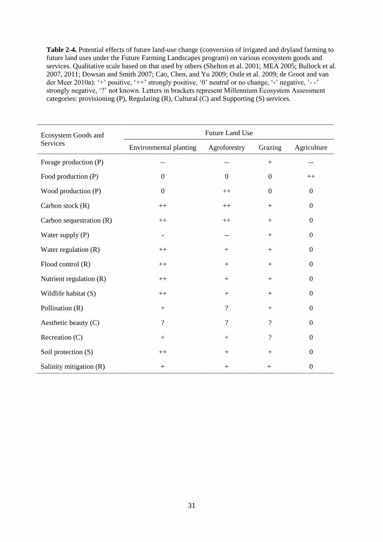
31

Table 2-4. Potential effects of future land-use change (conversion of irrigated and dryland farming to

future land uses under the Future Farming Landscapes program) on various ecosystem goods and

services. Qualitative scale based on that used by others (Shelton et al. 2001; MEA 2005; Bullock et al.

2007, 2011; Dowsan and Smith 2007; Cao, Chen, and Yu 2009; Ostle et al. 2009; de Groot and van

der Meer 2010a): ‘+’ positive, ‘++’ strongly positive, ‘0’ neutral or no change, ‘-’ negative, ‘- -’

strongly negative, ‘?’ not known. Letters in brackets represent Millennium Ecosystem Assessment

categories: provisioning (P), Regulating (R), Cultural (C) and Supporting (S) services.

Ecosystem Goods and

Services

Future Land Use

Environmental planting Agroforestry Grazing Agriculture

Forage production (P) -- -- + --

Food production (P) 0 0 0 ++

Wood production (P) 0 ++ 0 0

Carbon stock (R) ++ ++ + 0

Carbon sequestration (R) ++ ++ + 0

Water supply (P) - -- + 0

Water regulation (R) ++ + + 0

Flood control (R) ++ + + 0

Nutrient regulation (R) ++ + + 0

Wildlife habitat (S) ++ + + 0

Pollination (R) + ? + 0

Aesthetic beauty (C) ? ? ? 0

Recreation (C) + + ? 0

Soil protection (S) ++ + + 0

Salinity mitigation (R) + + + 0

32

Figure 2-3. Possible land-use changes in the study area and associated trade-offs among ecosystem services.

Intensively managed croplands can potentially be converted to four different land uses which produces different

response to various EGS, (i) intensive agriculture relative to recent past intensive pasture will have no effect on

major EGS with this land-use change simply replacing forage production with food production, (ii)

environmental planting with native tree species will have a positive effect on native species richness and carbon

sequestration but reduce water availability, (iii) grazing (extensive) – an extensive form of grazing with

biodiversity consideration will potentially enhance native species richness and some carbon sequestration but

will reduce forage production and have no effect on water availability, and (iv) commercial agroforestry systems

will enhance wood production and carbon sequestration but have negative effects on native species richness and

water availability (figure inspired by Bullock et al. 2011).

33

2.5.3. LESSONS FROM TWO CASES STUDIES

The two examples presented here show that anthropogenic driven land-use change can alter the

ecosystem’s capacity to provide various EGS required for human well-being. In our study clearing of

native vegetation provided important benefits for early settlers, as provided for production of

ecosystem goods (e.g., timber, food production). However, replacement of deep-rooted perennial

woody vegetation for shallow rooted annual crop or modified pasture reduced the supply of many

regulating services, such as water regulation, soil protection and climate regulation (Jones et al. 2007;

Yapp, Walker, and Thackway 2010) and reduced habitat and conservation services. When assessing

EGS consumed by humans we have to delineate between the ends and means (Fisher and Turner

2008). Some EGS are considered to be intermediate services while others generate final benefit or

end. In our case, for example, timber production can provide intermediate benefits for carbon

sequestration/stock which depend on the use of the timber. However, timber itself can be used for

human benefits and becomes a final EGS (see Boyd and Banzhaf 2007; Fisher and Turner 2008).

Results also demonstrated that commercial plantations and restoration efforts can enhance the

provision of different EGS but the results are not always complementary and trade-offs are inevitable

(Bullock et al. 2011). Demands for many EGS are increasing due to the population growth, market

trend, and changes on societal preferences (MEA 2005; FAO 2007; Baral et al. 2013). The value of

different EGS to society also changes over time. As more basic needs for subsistence are met, or as

the knowledge of the importance of different services for longer-term survival increases, societies

have begun to place more value on services such as water quality or carbon sequestration (Baral et al.

2013).

Qualitative assessment of EGS benefits supplied from different types of land uses and land cover from

different parts of a landscape can be useful for initial assessment and scoping study. To this end, our

results presented here are indicative only and more rigorous assessment such as quantitative and

economic valuation are required for final assessment (see Baral et al. 2009; 2013).

34

2.6. KEY ISSUES ASSOCIATED WITH EGS IN CHANGING

LANDSCAPES

2.6.1. TRADE-OFFS, AND SYNERGIES

Trade-offs among EGS occur when an increase in one service leads to a decrease in one or more other

services, and represent important externalities in current approaches to EGS management (Rodriguez

et al. 2006; Bennett et al. 2009). Trade-offs in EGS can be classified along three axes: (a) spatial scale

– location of trade-offs, (b) temporal scale – timing of trade-offs, and (c) reversibility – the possibility

of perturbed EGS returning to an improved state (MEA 2005; Rodriguez et al. 2006). Typically,

trade-offs among EGS arise from management choices and specific management practices made by

human society that can change the nature, magnitude and direction of services provided by

ecosystems (MEA 2005; Rodriguez et al. 2006).

Synergies occur when services either increase or decrease due to simultaneous response to the same

driver or due to true interactions among services (Bennett et al. 2009; Chattere and Agrawal 2009).

For example, a synergistic relationship exists among wildlife habitat and recreation opportunities in

protected areas such as national parks and wildlife reserves. The protected areas provide better habitat

for wildlife and also enhance opportunities for recreation and ecotourism (Lindsey et al. 2007). In

assessing trade-offs and synergies between alternative uses of ecosystems, the total bundle of EGS

provided by different conversion and management states need to be considered (Braat and de Groot

2012).

A number of researchers have studied the trade-off between two products and services provided by

forested ecosystems such as timber production and carbon sequestration (Seidl et al. 2007) and,

multiple EGS (Nelson et al. 2009; Raudsepp-Hearne, Peterson, and Bennett 2010). They found that

trade-offs are inevitable in many cases. Chattere and Agrawal (2009) analysed the relationships

between institutional factors and multiple benefits such as carbon storage and livelihood options using

35

original data for 10 countries across Asia, Africa, and Latin America. They found that larger forest

size and greater rule-making autonomy at the local level are associated with high carbon storage and

livelihood benefits and differences in ownership of forest are associated with trade-offs between

livelihood benefits and carbon storage.

2.6.2. PAYMENTS FOR ECOSYSTEM SERVICES

Payments for private ecosystem goods (e.g., food and timber) have commonly occurred in markets

throughout human history. However public services (e.g., fresh air, recreation) do not receive price

signals in markets and hence there are little financial incentives for landowners to produce them

(Ribaudo et al. 2010). Payments for ecosystem services (PES) are part of a new and more direct

conservation paradigm, explicitly recognising, (i) the need to bridge the interests of landowners and

the broader society, (ii) the costs of providing different ecosystem services, and (iii) that those that

benefit from these services to pay these costs. The underlying idea of PES is that EGS beneficiaries

(which may include individuals elsewhere, firms or broader community through the government)

make direct, contractual and conditional payments to local landholders in return for adopting practices

that provide increased services, for example through ecosystem conservation and restoration. A

number of financial incentives or PES type payment mechanisms are in place and have been practiced

in south-eastern Australia for some time. These have been generally described as market-based

instruments (MBIs) and include approaches such as Eco-Tender (Eigenraam et al. 2006), Bush Tender

(Stoneham et al. 2003) and Bio-banking (Burgin 2008). Such financial incentives can have both

synergies and tensions for land use and management practices which ultimately results in a range of

trade-offs and co-benefits across multiple EGS (see Bryn 2013).

Establishing a baseline and a quantified measure of EGS following the payment or credit transaction

are key requirement for any successful PES or MBIs (Patterson and Coelho 2009).

36

2.7. CONCLUDING COMMENTS

This review and initial analysis for two case study areas indicated that measuring EGS is a vital step

for valuation to guide management and for payments to provide incentives for the maintenance or

enhanced provision of currently unpriced ecosystem services such as water quality, carbon

sequestration or biodiversity conservation. However, multiple and complex definitions and

classification systems for EGS are often confusing for decision and policy makers. This confusion is

likely to be counterproductive in building the case for investment in measures to reduce land or

vegetation degradation and enhance the provision of ecosystem services (Wallace 2008). In addition,

the inconsistency in methods to assess and map EGS is a challenge for their inclusion in national

accounts and broader policy and natural resource management decision making (Crossman, Burkhard,

and Nedkov 2012). Furthermore, ongoing land use-land cover and climate change place further

complexity on future measurement and management of multiple EGS.

The case studies highlight the impact of land-use change on provision of EGS in south-eastern

Australia. Such land-use changes are similar to those occurring elsewhere, particularly in sub-tropical

or temperate developing regions. Our findings therefore have broader relevance, although we

recognise that the impacts of land-use changes on EGS will depend on local circumstances. Assessing

EGS supplied from different types of land uses and land cover from different parts of a landscape, and

identifying who benefits from these services, are critical steps in the development of effective land

use policy and decision-making. Spatially explicit, up-to-date and reliable information about EGS are

required to support this assessment.

37

2.8. REFERENCES

Acevedo, P., M. Á. Farfán, A. L. Márquez, M. Delibes-Mateos, R. Real, and J. M. Vargas. 2010.

“Past, Present and Future of Wild Ungulates in Relation to Changes in Land Use.” Landscape

Ecology 26 (1): 19–31.

Baral, H., R. J. Keenan, J. C. Fox, N. E. Stork, and S. Kasel. 2013. “Spatial Assessment of Ecosystem

Goods and Services in Complex Production Landscapes: A Case Study from South-eastern

Australia.” Ecological Complexity 13 (1): 35–45.

Baral, H., S. Kasel, R. J. Keenan, J. C. Fox, and N. E. Stork. 2009. “GIS-based Classification ,

Mapping and Valuation of Ecosystem Services in Production Landscapes: A Case Study of

the Green Triangle Region of South-eastern Australia.” In Forestry : a Climate of Change, ed.

R. Thistlethwaite, D. Lamb, and R. Haines, Proceedings of the IFA Conference, Caloundra,

Queensland, Australia, 6‒10 September 2009.

Barbier, E. B., and G. M. Heal. 2006. “Valuing Ecosystem Services.” Ed. Earthscan. The Economists

Voice 3 (3): 54–78.

Bennett, L.T., P. M. Mele, S. Annett, and S. Kasel. 2010. “Examining Links Between Soil

Management, Soil Health, and Public Benefits in Agricultural Landscapes: An Australian

Perspective.” Agriculture, Ecosystems and Environment 139 (1‒2): 1–12.

Bennett, E. M., G. D. Peterson, and L. J. Gordon. 2009. “Understanding Relationships Among

Multiple Ecosystem Services.” Ecology Letters 12 (12): 1394–404.

Benson, J. S., and P. A. Redpath. 1997. “The nature of pre-European native vegetation in south-

eastern Australia : a critique of Ryan, D. G., Ryan, J. R. and Starr, B. J. (1995) The Explorers

and Early Settlers.” Cunninghamia 5: 285–328.

Bhagwat, S. A., and C. Rutte. 2006. “Sacred Groves: Potential for Biodiversity Management.”

Frontiers in Ecology and the Environment 4 (10): 519–524.

Boumans, R., and R. Costanza. 2008. “The Multiscale Integrated Earth Systems Model (MIMES):

The Dynamics, Modeling and Valuation of Ecosystem Services.” Ed. C. Van Bers, D. Petry,

and C. Pahl-Wostl. Biological Conservation 141 (2): 1–3.

38

Boyd, J., 2010. Ecosystem Services and Climate Adaptation. Resources for Future, Washington D C.

Braat, L. C., and R. de Groot. 2012. “The Ecosystem Services Agenda: bridging the Worlds of

Natural Science and Economics, Conservation and Development, and Public and Private

Policy.” Ecosystem Services: 1(1): 4–15.

Bryan, B. A., 2010. “Development and Application of a Model for Robust, Cost-effective Investment

in Natural Capital and Ecosystem Services.” Biological Conservation 143 (7): 1737–1750.

Bryan, B. A. 2013. “Incentives, land use, and ecosystem services: Synthesizing complex linkages.”

Environmental Science and Policy 27: 124–134.

Bryan, B. A., C. M. Raymond, N. D. Crossman, and D. H. Macdonald. 2010. “Targeting the

Management of Ecosystem Services Based on Social Values: Where, What, and How?”

Landscape and Urban Planning 97 (2): 111–122.

Bullock, J. M, J. Aronson, A. C Newton, R. F. Pywell, and J. M. Rey-Benayas. 2011. “Restoration of

Ecosystem Services and Biodiversity: Conflicts and Opportunities.” Trends in Ecology &

Evolution 26 (10): 541–549.

Bullock, J. M., R. F. Pywell, and K. J. Walker. 2007. “Long-term Enhancement of Agricultural

Production by Restoration of Biodiversity.” Journal of Applied Ecology 44 (1): 6–12.

Burgin, S. 2008. “BioBanking: An Environmental Scientist’s View of the Role of Biodiversity

Banking Offsets in Conservation.” Biodiversity and Conservation 17 (4): 807–816.

Burkhard, B., F. Kroll, S. Nedkov, and F. Müller. 2012a. “Mapping Ecosystem Service Supply,

Demand and Budgets.” Ecological Indicators 21: 17–29.

Burkhard, B., R. de Groot, R. Costanza, R. Seppelt, S. Erik Jørgensen, and M. Potschin. 2012b.

“Solutions for Sustaining Natural Capital and Ecosystem Services.” Ecological Indicators 21:

1–6.

Busch, M., A. L. Notte, V. Laporte, and M. Erhard. 2012. “Potentials of Quantitative and Qualitative

Approaches to Assessing Ecosystem Services.” Ecological Indicators 21: 89–103.

39

Cao, S., L. Chen, and X. Yu. 2009. “Impact of China’s Grain for Green Project on the Landscape of

Vulnerable Arid and Semi-arid Agricultural Regions: A Case Study in Northern Shaanxi

Province.” Journal of Applied Ecology 46 (3): 536–543.

Chan, K. M. A., M. R. Shaw, D. R. Cameron, E. C. Underwood, and G. C. Daily. 2006.

“Conservation Planning for Ecosystem Services.” PLoS Biology 4 (11): e379.

Chhatre, A., and A. Agrawal. 2009. “Trade-offs and Synergies between Carbon Storage and

Livelihood Benefits from Forest Commons.” Proceedings of the National Academy of

Sciences of the United States of America 106 (42): 17667–70.

Cork, S., D. Shelton, C. Binning, and R. Parry. 2001. “A Framework for Applying the Concept of

Ecosystem Services to Natural Resource Management in Australia.” In Third Australian

Stream Management Conference, Brisbane, Australia, 27‒29 August, 2001.

Cork, S., and W. Proctor. 2005. “Implementing a Process for Integration Research : Ecosystem

Services Project, Australia.” Journal of Research Practice 1 (2): 1–25.

Cork, S., G. Stoneham, and K. Lowe. 2007. Ecosystem Services and Australian Natural Resource

Management (NRM) Futures. Paper to the Natural Resource Policies and Programs

Committee (NRPPC) and the Natural Resource Management Standing Committee (NRMSC).

Australian Government Department of the Environment, Water, Heritage and the Arts,

Canberra.

Costanza, R., R. d’Arge, R. de Groot, S. Farber, M. Grasso, B. Hannon, K. Limburg, et al. 1997. “The

Value of the World’s Ecosystem Services and Natural Capital.” Nature 387 (6630): 253–260.

Costanza, R. 2008. “Ecosystem Services: Multiple Classification Systems Are Needed.” Biological

Conservation 141: 350–352.

Crossman, N. D., B. Burkhard, and S. Nedkov. 2012. “Quantifying and Mapping Ecosystem

Services.” International Journal of Biodiversity Science Ecosystem Services Management 8:

37–41.

40

Crossman, N. D., J. D. Connor, B. A. Bryan, D. M. Summers, and J. Ginnivan. 2010. “Reconfiguring

an Irrigation Landscape to Improve Provision of Ecosystem Services.” Ecological Economics

69 (5): 1031–1042.

Crossman, N. D., and B. A. Bryan. 2009. “Identifying Cost-effective Hotspots for Restoring Natural

Capital and Enhancing Landscape Multifunctionality.” Ecological Economics 68 (3): 654–

668.

Crossman, N. D., B. A. Bryan, and D. King. 2011. “Contribution of Site Assessment Toward

Prioritising Investment in Natural Capital.” Environmental Modelling & Software 26 (1): 30–

37.

Currie, B., S. J. Milton, and J.C. Steenkamp. 2009. “Cost–benefit Analysis of Alien Vegetation

Clearing for Water Yield and Tourism in a Mountain Catchment in the Western Cape of

South Africa.” Ecological Economics 68 (10): 2574–2579.

Daily, G. C., and P. A. Matson. 2008. “Ecosystem Services: From Theory to Implementation.”

Proceedings of the National Academy of Sciences of the United States of America 105 (28):

9455–9456.

Daily, G. C. 1997. Nature’s Services: Societal Dependence on Natural Ecosystems. Island Press:

Washington D. C.

Dale, V.H., and S. Polasky. 2007. “Measures of the Effects of Agricultural Practices on Ecosystem

Services.” Ecological Economics 64 (2): 286–296.

Daniel, T. C., A. Muhar, A. Arnberger, O. Aznar, J. W. Boyd, K. M. A. Chan, R. Costanza, et al.

2012. “Contributions of Cultural Services to the Ecosystem Services Agenda.” Proceedings of

the National Academy of Sciences of the United States of America 109 (23).

doi:10.1073/pnas.1114773109.

Dawson, J. J. C., and P. Smith. 2007. “Carbon Losses from Soil and Its Consequences for Land-use

Management.” Science of the Total Environment 382 (2‒3): 165–190.

41

De Groot, R.S., R. Alkemade, L. Braat, L. Hein, and L. Willemen. 2010. “Challenges in Integrating

the Concept of Ecosystem Services and Values in Landscape Planning, Management and

Decision Making.” Ecological Complexity 7 (3): 260–272.

De Groot, R. S., and P. J. van der Meer. 2010. “Quantifying and Valuing Goods and Services

Provided by Plantation Forests.” In Ecosystem Goods and Services from Plantation Forests,

ed. Jurgen Bauhus, Peter van der Meer, and Markku Kanninen, London: Earthscan.

De Groot, R. S., M. A. Wilson, and R. M. J. Boumans. 2002. “A Typology for the Classification,

Description and Valuation of Ecosystem Functions, Goods and Services.” Ecological

Economics 41 (3): 393–408.

De Groot, R., L. Brander, S. van der Ploeg, R. Costanza, F. Bernard, L. Braat, M. Christie, et al. 2012.

“Global Estimates of the Value of Ecosystems and Their Services in Monetary Units.”

Ecosystem Services 1 (1): 50–61.

Egoh, B. N., B. Reyers, M. Rouget, and D. M. Richardson. 2011. “Identifying Priority Areas for

Ecosystem Service Management in South African Grasslands.” Journal of Environmental

Management 92 (6): 1642–1650.

Eigenbrod, F., P. R. Armsworth, B. J. Anderson, A. Heinemeyer, S. Gillings, D. B. Roy, C. D.

Thomas, and K. J. Gaston. 2010. “The Impact of Proxy-based Methods on Mapping the

Distribution of Ecosystem Services.” Journal of Applied Ecology 47 (2): 377–385.

Eigenraam, M., L. Strappazzon, N. Lansdell, A. Ha, C. Beverly, and J. Todd. 2006. EcoTender:

Auction for Multiple Environmental Outcomes. Department of Primary Industries, Melbourne.

FAO, 2007. Paying Farmers for Environmental Service, Food and Agricultural Organisation, Rome.

Farber, S. 2002. “Economic and Ecological Concepts for Valuing Ecosystem Services.” Ecological

Economics 41 (3): 375–392.

Farber, S., R. Costanza, D. L. Childers, J. Erickson, K. Gross, M. Grove, C. S. Hopkinson, et al. 2006.

“Linking Ecology and Economics for Ecosystem Management.” BioScience 56 (2): 121–133.

Farley, J., and R. Costanza. 2010. “Payments for Ecosystem Services: From Local to Global.”

Ecological Economics 69 (11): 2060–2068.

42

Farley, J. 2008. “The Role of Prices in Conserving Critical Natural Capital.” Conservation Biology 22

(6): 1399–1408.

Fisher, B., R. K.Turner, and P. Morling. 2009. “Defining and Classifying Ecosystem Services for

Decision Making.” Ecological Economics 68 (3): 643–653.

Fisher, B, and R. K Turner. 2008. “Ecosystem Services: Classification for Valuation.” Biological

Conservation 141: 1167–1169.

Flannery, T. 1994. The Future Eaters. Reed Books, Melbourne.

Flannery, T. 1998. “A reply to Benson and Redpath (1997).” Cunninghamia 5: 779–781.

Foley, J., R. Defries, G. P. Asner, C. Barford, G. Bonan, S. R. Carpenter, F. S. Chapin, et al. 2005.

“Global Consequences of Land Use.” Science 309 (5734): 570–574.

Gee, K., and B. Burkhard. 2010. “Cultural Ecosystem Services in the Context of Offshore Wind

Farming: A Case Study from the West Coast of Schleswig-Holstein.” Ecological Complexity

7 (3): 349–358.

Grantham, H. S., K. A. Wilson, A. Moilanen, T. Rebelo, and H. P. Possingham. 2009. “Delaying

Conservation Actions for Improved Knowledge: How Long Should We Wait?” Ecology

Letters 12 (4): 293–301.

Grigg, A., Z. Cullen, J. Foxall, L. Crosbie, L. Jamison, and R. Brito. 2009. The Ecosystem Services

Benchmark. A Guidance Document, Fauna and Flora International, UNEP. Cambridge.

Haines-Young, R., M. Potschin, and F. Kienast. 2012. “Indicators of Ecosystem Service Potential at

European Scales: Mapping Marginal Changes and Trade-offs.” Ecological Indicators 21: 39–

53.

Haines-Young, R., and M. Potschin. 2009. “Methodologies for Defining and Assessing Ecosystem

Services.” Nottingham: University of Nottingham.

Hector, A., and R. Bagchi. 2007. “Biodiversity and Ecosystem Multifunctionality.” Nature 448

(7150): 188–190.

Jones, R. N., P. Dettmann, G. Park, M. Rogers, and T. White. 2007. “The Relationship Between

Adaptation and Mitigation in Managing Climate Change Risks: a Regional Response from

43

North Central Victoria, Australia.” Mitigation and Adaptation Strategies for Global Change

12 (5): 685–712.

Kareiva, P., H. Tallis, T. H. Ricketts, G. C. Daily, and S. Polasky. 2011. Natural Capital: Theory and

Practice of Mapping Ecosystem Services. Oxford University Press, New York.

Krueger, T., T. Page, K. Hubacek, L. Smith, and K. Hiscock. 2012. “The Role of Expert Opinion in

Environmental Modelling.” Environmental Modelling and Software 36: 4–18.

Kumar, M., and P. Kumar. 2008. “Valuation of the Ecosystem Services: A Psycho-cultural

Perspective.” Ecological Economics 64 (4): 808–819.

Lindsey, P. A., R. Alexander, M. G. L. Mills, S, Romanach, and R. Woodroffe. 2007. “Wildlife

Viewing Preferences of Visitors to Protected Areas in South Africa: Implications for the Role

of Ecotourism in Conservation.” Journal of Ecotourism 6 (1): 19–33.

Luck, Ga. W., K. M. A. Chan, and J. P. Fay. 2009. “Protecting Ecosystem Services and Biodiversity

in the World’s Watersheds.” Conservation Letters 2 (4): 179–188.

MacEwan, R., N. Robinson, M. Imhof, D. Rees, and V. Sposito. 2008. “Primary Production

Landscapes of Victoria.” In 14th Agronomy Conference, Adelaide, South Australia, 21–25

September 2008.

Mansergh, I. 2010. “North Central Victoria – Climate Change and Land-use: Potentials for Third

Century in a Timeless Land.” Proceedings of the Royal Society of Victoria 122 (2): 161–183.

Martínez-Harms, M. J., and P. Balvanera. 2012. “Methods for Mapping Ecosystem Service Supply: a

Review.” International Journal of Biodiversity Science, Ecosystem Services & Management 8

(1–2): 17–25.

Maynard, S., D. James, and A. Davidson. 2010. “The Development of an Ecosystem Services

Framework for South East Queensland.” Environmental Management 45 (5): 881–895.

MEA. 2005. Ecosystems and Human Well-being: Synthesis. Washington, D. C.: Island Press.

Nahlik, A.M., M.E. Kentula, M.S. Fennessy, and D.H. Landers. 2012. Where Is the Consensus? A

Proposed Foundation for Moving Ecosystem Service Concepts into Practice. Ecological

Economics 77: 27–35.

44

Naidoo, R., A. Balmford, R. Costanza, B. Fisher, R. E. Green, B. Lehner, T. R. Malcolm, and T. H.

Ricketts. 2008. “Global Mapping of Ecosystem Services and Conservation Priorities.”


9495–9500.

Nelson, E., G. Mendoza, J. Regetz, S. Polasky, H. Tallis, D. R. Cameron, K. M. A. Chan, et al. 2009.

“Modeling Multiple Ecosystem Services, Biodiversity Conservation, Commodity Production,

and Trade-offs at Landscape Scales.” Frontiers in Ecology and the Environment 7 (1): 4–11.

Nijkamp, P., G. Vindigni, and P. A. L. D Nunes. 2008. “Economic Valuation of Biodiversity : A

Comparative Study.” Ecological Economics 67: 217–231.

Of, N. 2008. “The Sacred Groves and their Significance in Conserving Biodiversity: An Overview.”

International Journal of Ecology and Environmental Sciences 34 (3): 277–291.

Ostle, N. J., P. E. Levy, C. D. Evans, and P. Smith. 2009. “UK Land Use and Soil Carbon

Sequestration.” Land Use Policy 26 (Supplement 1): S274–S283.

Patterson, T. M., and D. L. Coelho. 2009. “Ecosystem Services: Foundations, Opportunities, and

Challenges for the Forest Products Sector.” Forest Ecology and Management 257 (8): 1637–

1646.

Payne, C. R., and P. Sand. 2011. Environmental Liability: Gulf War Reparations and the UN

Compensation Commission. Oxford University Press, London and New York.

Pittock, J., S. Cork, and S. Maynard. 2012. “The State of the Application of Ecosystems Services in

Australia.” Ecosystem Services: 1–10. doi:10.1016/j.ecoser.2012.07.010.

Polasky, S., E. Nelson, D. Pennington, and K. A. Johnson. 2011. “The Impact of Land-Use Change on

Ecosystem Services, Biodiversity and Returns to Landowners: A Case Study in the State of

Minnesota.” Environmental and Resource Economics 48 (2): 219–242.

Proctor, W., S. Cork, J. Langridge, A. Langston, N. Abel, M. Howden, M. Anderies, R. Parry, and D.

Shelton. 2002. “Assessing Ecosystem Services in Australia.” In 7th Biennial Conference of

the International Society for Ecological Economics. Sousse, Tunisia.

45

Ramankutty, N., J. A. Foley, J. Norman, and K. McSweeney. 2002. “The Global Distribution of

Cultivable Lands: Current Patterns and Sensitivity to Possible Climate Change.” Global

Ecology and Biogeography 11 (5): 377–392.

Raudsepp-Hearne, C., G. D. Peterson, and E. M. Bennett. 2010. “Ecosystem Service Bundles for

Analyzing Trade-offs in Diverse Landscapes.” Proceedings of the National Academy of

Sciences of the United States of America 107 (11): 5242–5247.

Raymond, C.M., B. A. Bryan, D.H. MacDonald, A. Cast, S. Strathearn, A. Grandgirard, and T.

Kalivas. 2009. Mapping Community Values for Natural Capital and Ecosystem Services.

Ecological Economics 68 (5): 1301–1315.

Ribaudo, M., C. Greene, L. Hansen, and D. Hellerstein. 2010. “Ecosystem services from agriculture:

steps for expanding markets.” Ecological Economics 69: 2085–2092.

Rodríguez, J. P., T. D. Beard, E. M. Bennett, G. S. Cumming, S. J. Cork, J. Agard, A. P. Dobson, and

G. D. Peterson. 2006. “Trade-offs Across Space, Time, and Ecosystem Services.” Ecology

and Society 11 (1): 28.

Rudel, T. K., L. Schneider, M. Uriarte, B. L. Turner, R. DeFries, D. Lawrence, J. Geoghegan, et al.

2009. “Agricultural Intensification and Changes in Cultivated Areas, 1970–2005.”


20675–20680.

Ryan, D. G., J. E. Ryan, B. J. Starr. 1995. The Australian landscape – observations of explorers and

early settlers, Murrumbidgee Catchment Management Committee: Wagga Wagga NSW.

Salles, J., 2011. “Valuing Biodiversity and Ecosystem Services: Why Put Economic Values on

Nature?” Comptes Rendus Biologies 334 (5–6): 469–482.

Scolozzi, R., and D. Geneletti. 2012. “Assessing Habitat Connectivity for Land-use Planning: a

Method Integrating Landscape Graphs and Delphi Survey.” Journal of Environmental

Planning and Management (21): 1–18.

Seidl, R., W. Rammer, D. Jager, W. Currie, and M. Lexer. 2007. “Assessing Trade-offs Between

Carbon Sequestration and Timber Production within a Framework of Multi-purpose Forestry

in Austria.” Forest Ecology and Management 248 (1–2): 64–79.

46

Shelton, D., S. Cork, C. Binning, R. Parry, P. Hairsine, and R. Vertessy. 2001. “Application of an

Ecosystem Services Inventory Approach to the Goulburn Broken Catchment.” In Third

Australian Stream Management Conference, Brisbane, Queensland, 27‒29 August 2001.

Sherrouse, B. C., J. M. Clement, and D. J. Semmens. 2011. “A GIS Application for Assessing,

Mapping, and Quantifying the Social Values of Ecosystem Services.” Applied Geography 31

(2): 748–760.

Steffen, W., A. A. Burbidge, L. Hughes, R. Kitching, W. Lindenmayer, D. Musgrave, M. S. Smith,

and P. A. Werner. 2009. Australia’s Biodiversity and Climate Change. CSIRO Publishing,

Melbourne.

Stoneham, G., V. Chaudhri, A. Ha, and L. Strappazzon. 2003. “Auctions for Conservation Contracts:

An Empirical Examination of Victoria’s Bush Tender Trial.” The Australian Journal of

Agricultural and Resource Economics 47 (4): 477–500.

Tallis, H. T., T. Ricketts, E. Nelson, D. Ennaanay, S. Wolny, N. Olwero, K. Vigerstol, et al. 2011.

InVEST 1.0 Beta User’s Guide. The Natural Capital Project Stanford. The Natural Capital

Project.

TEEB. 2009. “TEEB for National and International Policy Makers. Summary: Responding to the

Value of Nature”. UNEP, Geneva.

TEEB. 2010. The Economics of Ecosystems and Biodiversity: Mainstreaming the Economics of

Nature: A Synthesis of the Approach, Conclusions and Recommendations of TEEB. Geneva.

Turner, R. K., S. Morse-Jones, and B. Fisher. 2010. “Ecosystem Valuation: a Sequential Decision

Support System and Quality Assessment Issues.” Annals of the New York Academy of

Sciences 1185: 79–101.

Vihervaara, P., T. Kumpula, A. Ruokolainen, and A. Tanskanen. 2012. “The Use of Detailed Biotope

Data for Linking Biodiversity with Ecosystem Services in Finland.” International Journal of

Biodiversity Science, Ecosystem Services & Management 8 (1–2): 169–185.

47

Vihervaara, P., A. Marjokorpi, T. Kumpula, M. Walls, and M. Kamppinen. 2011. “Ecosystem

Services of Fast-growing Tree Plantations: A Case Study on Integrating Social Valuations

with Land-use Changes in Uruguay.” Forest Policy and Economics 14 (1): 58–68.

Vihervaara, P., T. Kumpula, A.Tanskanen, and B. Burkhard. 2010. “Ecosystem services–A Tool for

Sustainable Management of Human–environment Systems. Case Study Finnish Forest

Lapland.” Ecological Complexity 7 (3): 410–420.

Villa, F., K. Bagstad, G. Johnson, and B. Voigt. 2011. “Scientific Instruments for Climate Change

Adaptation: Estimating and Optimizing the Efficiency of Ecosystem Service Provision.”

Economía Agrariay Recursos Naturales 11 (1): 83–98.

Villa, F., M. Ceroni, K. Bagstad, G. Johnson, and S. Krivov. 2009. “ARIES (ARtificial Intelligence

for Ecosystem Services): a New Tool for Ecosystem Services Assessment , Planning , and

Valuation.” In Economic Instruments to Enhance the Conservation and Sustainable Use of

Biodiversity, Venice.

Walker, B. H., N. Abel, J. M. Anderies, and P. Ryan. 2009. “Resilience, Adaptability, and

Transformability in the Goulburn–Broken Catchment, Australia.” Ecology and Society 14 (1):

12.

Wallace, K. 2007. “Classification of Ecosystem Services: Problems and Solutions.” Biological

Conservation 139 (3–4): 235–246.

Wallace, K. 2008. “Ecosystem Services: Multiple Classifications or Confusion?” Biological

Conservation 141 (2): 353–354.

Wilson, K. A., E. Meijaard, S. Drummond, H. S. Grantham, L. Boitani, G. Catullo, L. Christie, et al.

2010. “Conserving Biodiversity in Production Landscapes.” Ecological Applications 20 (6):

1721–1732.

Yapp, G., J. Walker, and R. Thackway. 2010. “Linking Vegetation Type and Condition to Ecosystem

Goods and Services.” Ecological Complexity 7 (3): 292–301.

48

Zak, M. R., M. Cabido, D. Cáceres, and S. Díaz. 2008. “What Drives Accelerated Land Cover Change

in Central Argentina? Synergistic Consequences of Climatic, Socioeconomic, and

Technological Factors.” Environmental Management 42 (2): 181–189.

49

Table S2-1. Major classification systems of ecosystem goods and services.

Costanza et al. (1997) Daily (1997) Cork et al. (2001) MEA (2005) Wallace (2007) TEEB (2009) de Groot et al. (2010b)

Definition

the benefits human

populations derive,

directly or indirectly,

from ecosystem

functions

the conditions and

processes through

which natural

ecosystems, and the

species that make

them up, sustain and

fulfill human life

use Daily (1997) the benefits

people obtain

from ecosystems

use MEA (2005) the direct and

indirect

contributions of

ecosystems to

human well-being

use MEA (2005)

Classification system

food production (e.g.

fish, game, fruit)

food pollination food food food food

raw materials durable materials

(natural fibre, timber)

life-fulfilling

services

fibre oxygen raw materials fibre, fuel other raw

materials

water supply energy (biomass

fuels)

regulation of

climate

fuel water water biochemical products

and medicinal

resources

gas regulation industrial products pest control genetic resources energy genetic resources ornamental species

and/or resources

waste treatment pharmaceuticals genetic resources biochemicals,

natural medicines

dispersal aids medicinal resources genetic materials

erosion control and

sediment retention

genetic resources maintenance and

regeneration of

habitat

ornamental

resources

protection from

predators

ornamental

resources

water

pollination genetic resources provision of shade

and shelter

freshwater protection from

disease and parasites

air quality

regulation

air quality regulation

disturbance

regulation

cycling and filtration

processes

filtration and

erosion control

air quality

regulation

temperature climate regulation water regulation

climate regulation translocation

processes (dispersal

of seeds, pollination)

maintenance of

soil health

climate regulation moisture moderation of

extreme events

waste treatment

biological control regulation of

hydrological cycle

regulation of river

flows and

groundwater

levels

water regulation chemical waste treatment erosion protection

50

nutrient cycling river channel stability waste absorption

and breakdown

erosion regulation spiritual and

philosophical

contentment

erosion prevention pollination

soil formation moderation of

weather extremes

water purification

and waste

removal

benign social group maintenance of soil

fertility

natural hazard

mitigation

refugia partial stabilization of

climate

disease regulation recreation/leisure pollination climate regulation

recreation control of pest

species

pest regulation meaningful

occupation

biological control biological regulation

cultural aesthetic beauty pollination aesthetics maintenance of life

cycles of migratory

species

soil formation and

regeneration

cultural, intellectual

and spiritual

inspiration

natural hazard

regulation

opportunity values maintenance of

genetic diversity

genepol protection

scientific discovery cultural diversity aesthetic

information

nursery habitat

serenity spiritual and

religious values

opportunities for

recreation &

tourism

recreation and tourism

existence value knowledge

systems

inspiration for

culture, art and

design

cultural heritage and

identity

maintenance of the

ecological

components and

systems needed for

future supply

educational values spiritual experience aesthetic

inspiration information for

cognitive

development

inspiration for culture

art and design

aesthetic values spiritual and religious

inspiration

social relations education and science

51

CHAPTER 3: SPATIAL ASSESSMENT OF ECOSYSTEM GOODS AND

SERVICES IN COMPLEX PRODUCTION LANDSCAPES: A CASE STUDY FROM

SOUTH-EASTERN AUSTRALIA

This chapter has been published as follows:

Baral, H., Keenan, R.J., Fox, J.C., Stork, N.E., Kasel, S., 2013. Spatial assessment of ecosystem goods and

services in complex production landscapes: A case study from south-eastern Australia. Ecological Complexity

13, 35–45.

3.1. ABSTRACT

Many production landscapes are complex human-environment systems operating at various spatio-

temporal scales and provide a variety of ecosystem goods and services (EGS) vital to human well-

being. EGS change over space and time as a result of changing patterns of land use or changes in the

composition and structure of different vegetation types. Spatio-temporal assessment of EGS can

provide valuable information on the consequences of changing land use and land cover for EGS and

helps to deal with this complexity. We carried out a quantitative and qualitative appraisal of selected

EGS (timber production, carbon stock, provision of water, water regulation, biodiversity, and forage

production) to understand how these have altered in a complex mosaic of landscape that has

undergone significant change over the past 200 years.

Land use and land cover types and their associated EGS were assessed and mapped using a wide

range of readily available data and tools. We also evaluated the trade-offs among services associated

with observed land use change. In contrast to work elsewhere, we found the recent changes in land

use and land cover have an overall positive impact on various EGS due mainly to the conversion of

pasture to managed plantations which are connected to the larger areas of remnant vegetation. Results

also indicate that there was a high level of variation in the distribution of the EGS across the

landscape. Relatively intact native vegetation provide mainly regulating services whereas the

modified landscapes provides provisioning services such as timber and forage production at the cost

52

of regulating services. Rapidly changing demand and supply of certain goods and services (e.g.,

timber, pulp or carbon) may also have positive and negative impact on other services. For example,

increasing plantation rotation has positive impacts for biodiversity and carbon stock but reduces

stream flow and water yield.

3.2. INTRODUCTION

In recent years, understanding the value of ecosystem goods and services (EGS), through their

description and quantification, particularly in rapidly changing landscapes, has become widely

recognised as important areas of study (Fisher et al., 2009). The Millennium Ecosystem Assessment

(MEA) strongly linked ecosystem health with human welfare and identified that at the global scale 15

out of 24 recognised EGS are in a state of decline (MEA, 2005). The MEA looked at four possible

future scenarios on how EGS (under four categories: provisioning, regulating, cultural and supporting

services) might change in the future and their implications for human well-being (Burkhard et al.,

2010; Carpenter et al., 2006; MEA, 2005). Elsewhere, other modelled scenarios consistently indicate

that EGS will continue to decline in the 21st century with likely negative impacts on human welfare

(Pereira et al., 2010). However, most such analyses have focused on intact natural vegetation and

there has been less attention to the assessment of EGS in the more complex production landscapes

that support dynamic mosaics of agriculture, pastures, managed plantations and native remnant

vegetation.

If planned and managed appropriately, production landscapes can support not only the production of

food and fibre but also a wide variety of non-market services such as biodiversity conservation, water

regulation, and landscape amenity (Eigenbrod et al., 2009; Lovell and Johnston, 2009a, 2009b; Power,

2010; Verburg et al., 2009). Quantification, mapping and valuation of multiple EGS in production

landscapes are therefore of considerable interest for environmental policy and land management as

different configurations of landscapes and mixtures of production versus conservation may be more

53

productive than others (Bennett and Balvanera, 2007; Cork et al., 2007; O’Farrell et al., 2010;

Petrosillo et al., 2009). Assessment and mapping of EGS are considered essential prerequisites to

subsequent quantification and valuation (Burkhard et al., 2010, 2012; de Groot et al., 2010; Kareiva et

al., 2011). Importantly, spatially explicit assessment of EGS can be helpful in analysing trade-offs and

synergies among EGS in a particular landscape (Naidoo et al., 2008; Nelson et al., 2009; Raudsepp-

Hearne et al., 2010).

Production landscapes are characterised by complex inter-relations between biophysical, socio-

economic, and culturally heterogeneous components that interact at several spatio-temporal scales

(Cadenasso et al., 2006; Petrosillo et al., 2010). Moreover, they are subject to regular human

intervention as well as natural disturbances (Bennett and Balvanera, 2007; Burkhard et al., 2012;

Carpenter et al., 2006) and present different challenges to assessing EGS than intact natural systems.

Over the past 200 years large parts of the Australian landscapes have been intensively modified to

provide food and fibre (Steffen et al., 2009). The effect of this modification and large-scale clearing

has commonly resulted in the degradation of land and water resources (de Groot, 2006) which has

affected other EGS such as biodiversity, water quality and gas regulation (Steffen et al., 2009).

Victoria is the most extensively cleared Australian state and has also been subject to the longest

history of human use (Beeton et al., 2006). Victoria comprises a rich variety of terrestrial ecosystems

which result from a diversity of terrain, climate, geology and soil types (MacEwan et al., 2008). Over

recent decades, land use practices have changed significantly and have been modified to suit this

diversity of climate and soil. While the value of commodities produced from production landscapes

has been recognised since the beginning of settled agriculture, it is becoming increasingly important

to understand the wider uses and benefits that production landscapes provide society (Bennett et al.,

2009; Dale and Polasky, 2007).

The value of EGS is determined by the beneficiaries of the particular EGS (Bennett et al., 2010;

Fisher et al., 2009). These can vary from local land owners and communities to purchasers or users of

EGS in other parts of a catchment, or in national or global markets. The nature of the benefit also

54

varies. Those purchasing goods are generally receiving a private benefit resulting from their personal

use of these goods. For services such as water regulation, carbon stock or biodiversity, there are

shared or public benefits associated with the potentially wide access to these benefits from a range of

different beneficiaries. Beneficiaries may also extend to future generations. In some cases there are

market-based processes developing to facilitate investment in the provision of services such as

increased carbon sequestration or improved water quality (DPI, 2005). The value that the local and

global communities place on different types of EGS also changes over time (Costanza, 2008; Daily et

al., 2009; Fisher et al., 2009). As more basic needs for subsistence are met, or as the knowledge of the

importance of different services for longer-term survival increases, societies have begun to place more

value on services such as water quality or carbon sequestration.

This study aimed to characterise EGS produced from various land use/cover types within a production

landscape and to assess the change in supply of these over time as a result of land use change. We

carried out a quantitative and qualitative appraisal for selected EGS (timber production, carbon stock,

provision of water, water regulation, biodiversity, and forage production) and developed a quantitative

framework to evaluate the effects of land use and land cover change in the past 200 years on these

EGS. We chose a study area subject to a relatively high rate of change in land use and land cover,

primarily in recent years through conversion of agricultural land to intensively-managed forest

plantations. These changes can have both positive and negative impacts on different types of EGS at

local and regional scales over time (Brockerhoff et al., 2008). This ‘spatio-temporal dynamic’

presents a further challenge in understanding and classifying EGS produced from complex landscapes

(Cadenasso et al., 2006; Fisher et al., 2009).

55

3.3. METHODS

3.3.1. REVIEW – ASSESSMENT AND MAPPING OF EGS

Methodologies used for identifying, assessing and mapping EGS are diverse and often inconsistent.

Similarly the spatial representation, objective of mapping, and number of EGS assessed and mapped

varied widely. Some recent examples of EGS assessment and mapping are summarised in Table 3-1.

Assessing and mapping the distribution of multiple EGS is difficult due to lack of data (Naidoo et al.,

2008; Seppelt et al., 2011) and two possible solutions identified from a number of recent studies are to

either; (i) use expert opinion to rank the relative capacity of EGS (e.g. Burkhard et al., 2009, 2012;

Nedkov and Burkhard, 2012; Vihervaara et al., 2010; Yapp et al., 2010) or (ii) estimate values using

proxies (e.g., Luck et al., 2009; Turner et al., 2007). In this study, we assess and map six important

EGS provided by a production landscape using a mixed approach (Fig. 1-1).

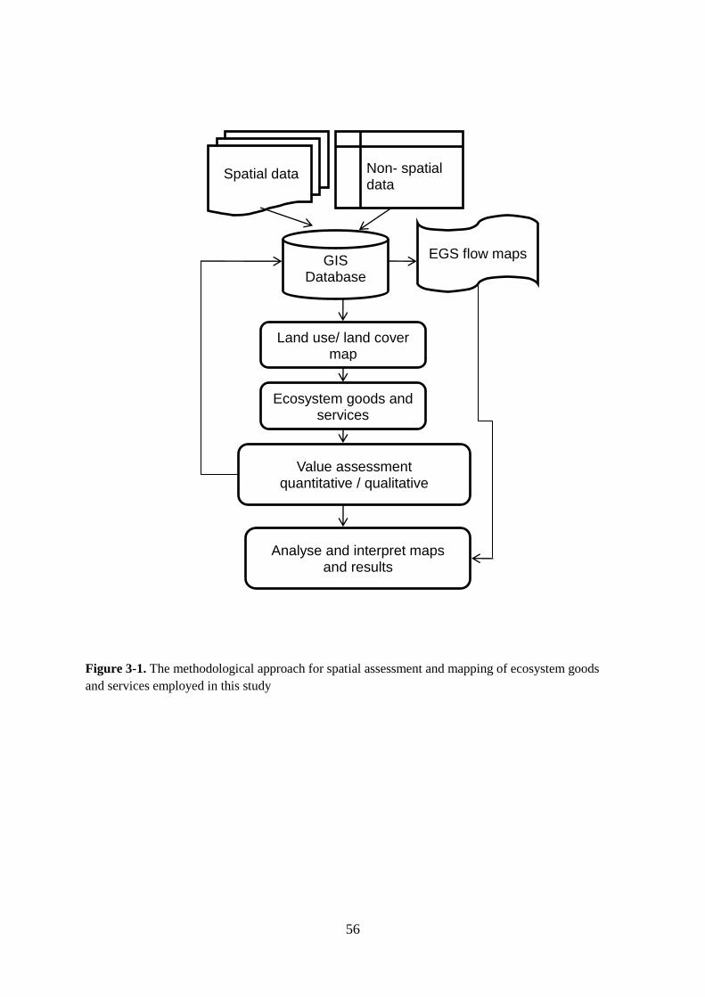
56

Figure 3-1. The methodological approach for spatial assessment and mapping of ecosystem goods

and services employed in this study

Ecosystem goods and services

Spatial data Non- spatial data

GIS Database

Land use/ land cover map

Value assessment quantitative / qualitative

Analyse and interpret maps and results

EGS flow maps

57

Table 3-1. A summary of recent studies on assessment and mapping of ecosystem goods and services (EGS)

Location Method and objectives EGS assessed and mapped Reference

Leipzig-Halle,

Germany

easy-to-apply concept based on a matrix linking spatially

explicit biophysical landscape to EGS for appropriate

quantification and spatial visualisation of EGS

22 EGS based on MEA categories Burkhard et al.

(2012)

Central Coast

ecoregion, California,

USA

use of spatially explicit conservation planning

framework to explore the trade-offs and opportunities for

aligning conservation goal for biodiversity and EGS

carbon stock, flood control, forage production,

outdoor recreation, crop pollination, water

provision

Chan et al.

(2006)

South Africa use of statistical distribution of proxy indicators to

quantify the amount an distribution of EGS across the

landscape and spatial congruence

water supply, water flow regulation, soil

accumulation, soil retention, carbon stock

Egoh et al.

(2008)

Ewaso Ngiro

Catchment, Kenya

mapping bundles of EGS at the land use scale for land

use planning and management in data-poor regions

carbon, wildlife species, timber, livestock, crops,

freshwater, flood regulation, cultural value

Erickson et al.

(2012)

Global watersheds spatial distribution of multiple ecosystem services for

reconciling conservation and human development goals

water provision, flood mitigation, carbon storage,

biodiversity priorities

Luck et al.

(2009)

Willamette Basin,

Oregon, USA

combination of land use and land cover classification

with a suite of models to map EGS

water quality, soil conservation, storm peak

management, carbon sequestration, biodiversity

conservation, commodity production

Nelson et al.

(2009)

Quebec, Canada mapped spatial distribution of proxy indicators for

selected EGS and identified bundles using spatial

location

crops, pork, drinking water, maple syrup, deer

hunting, nature appreciation, carbon

sequestration, soil retention, soil organic matter

Raudsepp-

Hearne et al.

(2010)

Little Karoo Region,

South Africa

use of land cover data as the basis for identifying EGS

and mapped the overlap in provision of EGS

forage production, carbon stock, erosion control,

tourism, water regulation

Reyers et al.

(2009)

Finish Forest Lapland,

Finland

effect of various land uses on provision of EGS using

GIS techniques

27 EGS based on MEA categories Vihervaara et al.

(2010)

58

3.3.2. STUDY SITE

The study area was the 300 km2 sub-catchment G8 of the Lower Glenelg Basin, in the Green Triangle

region of south-western Victoria (8-198 m asl, 37º 50’ S, 141º 30’ E; Fig. 3-2). It was selected

because of its concentration of commercially valuable hardwood (Eucalyptus globulus) and softwood

(Pinus radiata) plantations (37% cover) within a mix of other land cover and land use types including

native vegetation (44%) and pasture (17%). Most of the softwood plantations have been established

since 1970s for sawlog production with a rotation of about 30 to 40 years. A large proportion of the

softwood plantation (67%) is matured or semi-matured (>20 years) and remaining is either mid-

rotation (16%; 5-20 years) or young (17%; <5 years). Hardwood plantations were established since

1990 and are nearly all Eucalyptus globulus grown for pulpwood on a rotation of 10 to 12 years.

Similar to softwood, large proportion of hardwood plantations (70%) is matured or semi-matured (8-

12 years), 28% is mid-rotation (4-8 years) and small proportion (2%) is young (<4 years). Other land

uses such as residential development, roads and mining comprise a small proportion of the landscape

and were not assessed in this study. The study area has a mean annual rainfall of approximately 700

mm and mean annual temperature of 8 ºC (min) to 19 ºC (max).

Since European settlement in the early 1850s, 50% (15,800 ha) of native vegetation in the study area

has been cleared. The proportion of remnant native vegetation is slightly higher than for Victoria as a

whole (46.2%) of the original extent (VEAC, 2010). Most remnant native vegetation is on public land,

including State Forests or other protected areas. The majority of remaining native vegetation

(classification follows DSE, 2011) and proportion of the area occupied within the study area are –

heathy woodlands (27%), plain woodlands (19%), herb-rich woodlands (9%), lowland forests(4%),

riparian or swampy scrubs (2%), heathlands (2%), riverine grassy woodlands (<1%) and wetlands

(<1%). The vegetation types that had the largest areas cleared are mainly eucalypt woodlands, and

eucalypt tall open forests. In contrast, large proportions of heathlands, riparian scrubs or swampy

scrubs remain (Fig. 3-2).

59

According to the Victorian Department of Sustainability and Environment’s (DSE) threatened flora

and fauna databases, 15 species of threatened flora and 26 different species of threatened fauna are

recorded for the study area, including 15 birds, five mammals, three amphibians and one reptile.

Seven species are classified as endangered, 11 as vulnerable and nine species are classified as near

threatened. Almost all threatened species are confined to the native vegetation except for one plant

species (Theymitra mucida), three faunal species recorded in managed plantation, and four faunal

species (two species of arboreal mammals and two species of waterbirds) recorded in pastures.

3.3.3. APPROACH

A general list of EGS applicable to the study area was derived based on those identified by Cork et al.

(2007), Costanza (2008), de Groot et al. (2002, 2010), and MEA (2005), (Table 3-2). For this study

we focused on selected EGS which are considered to be most important to this region but that are also

of wider national and international significance – timber production, carbon stock, provision of water,

water regulation, biodiversity, and forage production (Carpenter et al., 2009; Naidoo et al., 2008).

Rationales and a brief description of each EGS are provided below with further details on quantitative

and qualitative assessment criteria, beneficiary and associated spatial and temporal scales summarised

in Table 3-2 (see also Appendix 3-1 for further details).

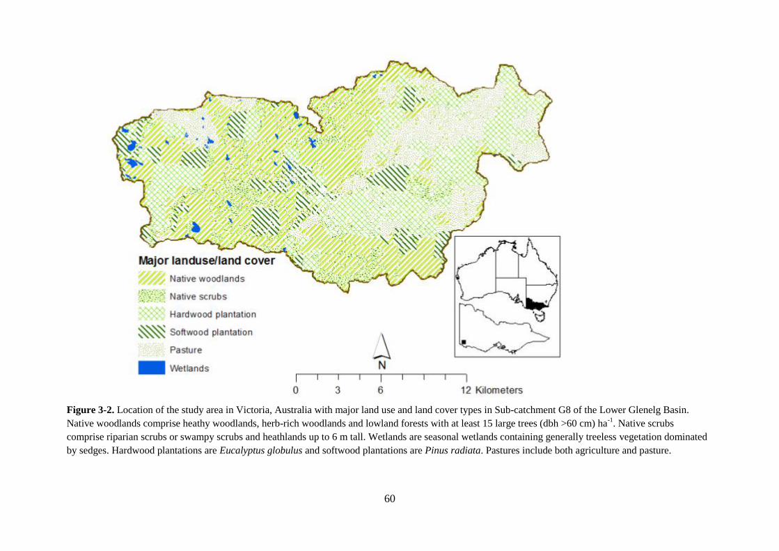
60

Figure 3-2. Location of the study area in Victoria, Australia with major land use and land cover types in Sub-catchment G8 of the Lower Glenelg Basin.

Native woodlands comprise heathy woodlands, herb-rich woodlands and lowland forests with at least 15 large trees (dbh >60 cm) ha-1

. Native scrubs

comprise riparian scrubs or swampy scrubs and heathlands up to 6 m tall. Wetlands are seasonal wetlands containing generally treeless vegetation dominated

by sedges. Hardwood plantations are Eucalyptus globulus and softwood plantations are Pinus radiata. Pastures include both agriculture and pasture.

61

Table 3-2. Key ecosystem goods and services (EGS) identified for sub-catchment G8, Lower Glenelg basin. Letters in brackets represent MEA ecosystem service categories:

provisioning (P), regulating (R), cultural (C) and supporting (S) services. Criteria range and codes for scale and time lag are adapted from Bennett et al. (2010): ‘O’ on-site

(in situ delivery), ‘L’ local (off-site, 100 m – 10 km), ‘R’ regional (10-1000 km), ‘G’ global (>1000 km) and time lag ‘I’ immediate (<1 year), ‘F’ fast (1 year to ≤10 years),

‘M’ medium (11 to ≤30 years), ‘S’ slow (31 to ≤50 years), ‘VS’ very slow (>50 years). Only the selected EGS in bold are assessed and mapped in this study. ‘DSE’ Dry

Sheep Equivalent which is equivalent to 0.125 Large Stock Unit (LSU)

EGS Description Beneficiary/use Scale Time lag Unit of measurement

Timber production

(P)

Provision of timber, pulp from managed plantations and native

production forests

Private O M m3 or tons ha

-1

Carbon stock (R) Stock of carbon in wood, other biomass and soil and keep CO2

out of the atmosphere

Public/Private O-R F-VS Mg ha-1

Provision of Water

(P)

Filtering, retention and storage of freshwater available for

human consumption or industrial use

Public O-R F-VS ML ha-1

yr-1

Water regulation (R) Role of land cover in regulating hydrological flows by

vegetation

Public /Private O-R M-VS m3 ha

-1

Biodiversity (S) Landscapes capacity to hold naturally functioning ecosystems

support a diversity of plant and animal life

Public/Private O-R I-VS

Forage production (P) Production of forage for domestic livestock mainly from pasture

and grazing land

Private O I-F DSE ha-1*

Carbon sequestration

(R)

Capture atmospheric carbon dioxide in trees, shrubs and other

vegetation

Public O-G F-VS Mg ha-1

yr-1

Nutrient regulation (R) Internal cycling, processing and acquisition of nutrients by

vegetation and microorganisms

Private O-L I-VS kg ha-1

yr-1

Pollination (R) Pollination of wild plant species and harvested crops Private/Public O-R I-S Number of, or impact of

pollinating species

Aesthetic beauty (C) Attractive landscape features helps enjoyments of scenery Private/Public O-R F-S Presence of landscape

features

Recreation (C) Travel to natural ecosystems for eco-tourism, outdoor sport etc Public L-R I-VS N° of visitors yr-1

, $ ha-1

yr-1

Soil protection (S) Promotes agricultural productivity and the integrity of natural

ecosystems

Private/Public O-R F-VS ha yr-1

62

3.3.3.1. TIMBER PRODUCTION

Timber and other wood fibre are commercial products provided by forest plantations (Tallis et al.,

2010) that generate a significant revenue and employment to this region (ABARES, 2011). The value

of timber is realised at the time of commercial thinning or final clear fell but we used mean annual

increment (MAI) as an estimate of capacity to supply timber or wood fibre for hardwood and

softwood plantations. MAI was estimated using CABALA (Bhattaglia et al., 2004) and Farm Forestry

Toolbox (FFT) (Version 5.0, Private Forests Tasmania, 2009) with associated data/parameter sets

calibrated to the study region, and then classified this into three classes of timber production (see

Table 3-3). For native woodlands we used the average increment for these forest types derived from

the Victorian Forest Resource Inventory (Hamilton et al., 1999).

3.3.3.2. CARBON STOCK

Forest and grassland ecosystems store carbon in living vegetation, dead organic material and soils and

are an important part of the global carbon cycle (Tallis et al., 2010). Conversion of woody vegetation

to other forms of land cover results in carbon emissions to the atmosphere and increasing carbon

stocks in woody vegetation can reduce net emissions and contribute to climate change mitigation

objectives (DCC, 2008). Therefore carbon storage and sequestration are important ecosystem services

in Australia and globally (Carpenter et al., 2009). Following a number of previous studies (e.g.,

Chan et al., 2006; Egoh et al., 2008, 2010; Reyers et al., 2009; Kareiva et al., 2011) this study

mapped carbon storage a service because maintaining vegetation in a natural state provides a

service to society. This has been recognised in recent legislation in Australia for the Carbon Farming

Initiative and the Clean Energy Future package that provides the framework for a trading scheme to

reduce greenhouse gas emissions (DCCEE, 2011a). In this study, carbon stock was estimated and

mapped as Mg ha-1

for each land use/cover type. For managed plantations we used CABALA

(Battaglia et al., 2004) and the Carbon Farming Initiative (CFI) reforestation tool (DCCEE, 2011b)

63

using GIS data available from forestry companies. For native vegetation and pastures we derived

proxy values from relevant studies (Grierson et al., 1992; IPCC, 2006; Norris et al., 2010; Paul et al.,

2008, 2013).

3.3.3.3. PROVISION OF WATER

Provision of clean water is a vital service provided by healthy streams and landscapes in south-eastern

Australia. However, estimating accurate water use by forest plantations and various vegetation types

is a difficult undertaking. It is generally agreed that for a given rainfall, a forest uses more water than

pasture and agricultural land (Keenan et al., 2006, Zhang et al., 1999, 2001). The deeper roots of trees

give them greater access to water and also with the lower albedo and greater height and roughness,

trees tend to absorb more energy than pastures and other land uses (Benyon et al., 2007; van Dijk and

Keenan, 2007).

Woody vegetation can remove nutrient pollutants applied to agricultural systems from runoff and

reduce salinity input to streams where salts are stored in the landscape. However, woody vegetation

also uses a large proportion of rainfall compared to other land uses and reduce inflow to streams and

rivers compared with other forms of land cover (Zhang et al., 1999, 2001). In this study we assessed

only potential water supply as defined by de Groot et al. (2002) filtering, retention and storage of

freshwater (e.g. in aquifers) in each land use and land cover type. Water yield from different forms of

land cover was assessed based on the potential ground water recharge (mm yr-1

) for given rainfall

conditions from the studies within this study area (Benyon et al., 2007, 2009). The estimated values

(Table S3-1) were transferred to land use and land cover types into GIS environment and then

assigned to three classes (see Table 3-3).

64

Table 3-3. Quantitative and qualitative assessment criteria for ecosystem EGS ranking.

EGS Value

classes

Description Data source/Tools Confidence

level**

Timber

production

High High mean annual increment potential, >10 ha-1

yr-1

CABALA (Battaglia et al., 2004), Farm Forestry

Toolbox, existing data/reports

High

Medium Moderate mean annual increment, 2-10 ha-1

yr-1

Low Low mean annual increment, <2 ha-1

yr-1

Carbon stock High High carbon stock potential, >250 Mg ha-1

CABALA (Battaglia et al., 2004), IPCC 2006;

DCC 2008; URS Forestry 2008; CFI reforestation

tool (DCCEE, 2011b), Grierson et al. (1992)

High

Medium Moderate carbon stock potential, 50–250 Mg ha-1

Low Low carbon stock potential, <50 Mg ha-1

Provision of

water

High Low level of water use and high recharge potential, >30

% of annual precipitation

Benyon et al.(2007), Zhang (1999, 2001)

Moderate

Medium Moderate water use and moderate recharge potential,

10-30% of annual precipitation

Low High level of water use and low recharge potential,

<10% of annual precipitation

Water

regulation

High Potential high water regulation potential due to

established vegetation

Land use and land cover maps; Zhang et al.

(1999, 2001); Keenan et al. (2006)

Low

Medium Moderate level of vegetation cover and water regulation

potential

Low Low level of vegetation cover, e.g., agriculture/pasture

Biodiversity* High Relatively intact areas of native vegetation with rare,

threatened and endangered species and areas supporting

vulnerable habitat type, score>10

Spatial analysis of GIS data mainly EVC layers

from DSE (DSE, 2011) and plantation data,

review of Threatened Fauna and Flora

Low

Medium Native vegetation with relatively smaller patch sizes,

score 5-10

Low Other areas with highly fragmented native vegetation,

planted forest, and pastures, score <5

Forage

production

High Area allocated for forage production, i.e., managed

pastures, >10 DSE ha-1

Saul et al.(2009, 2011), Blackwood et al.(2006) Moderate

Medium Potential sites with medium forage production

potential, 2–10 DSE ha-1

Low Native vegetation with potential to be grazed, e.g.,

native scrubs, <2 DSE ha-1

*Biodiversity score was calculated using Tables S3-2 and S3-3, Appendix 3-1, ** Confidence levels follow Reyers et al. (2009)

65

3.3.3.4. WATER REGULATION

Water regulation is an important ecosystem service provided by natural vegetation in the study area

which provides the potential benefits of regulating runoff and flood mitigation to downstream water

users. The important role of upstream vegetation cover in ensuring the delivery of high-quality water

in downstream has been well recognised (Calder et al., 2007). However, due to lack of quantitative

data, this service was assessed qualitatively by reviewing relevant literature to the study region

(Brown et al., 2007; Keenan et al., 2006; Whirehead and Beadle, 2004; Zhang, 1999, 2001) into three

classes – high, moderate and low capacity of each land use and land cover types (Table 3-3).

3.3.3.5. BIODIVERSITY

Biodiversity can be valued by society for its intrinsic worth or for its contribution to the provision of

various additional EGS in the study area. Both natural and manmade ecosystems support certain

levels of biodiversity and recently a number of methods and tools have been made available for

biodiversity habitat condition assessment (Eyre et al., 2011; Parkes et al., 2003). Managed plantations

can support a greater abundance of native fauna and flora than agricultural land but are not

comparable to native vegetation (Brockerhoff et al., 2008; Felton et al., 2010; Kasel et al., 2008;

Kavanagh et al., 2005, 2007; Loyn et al., 2007; Munro et al., 2009). However, establishing plantations

on agricultural land may negatively affect species that prefer grasslands or open habitats, and the

edges of woodland (Davies et al., 2001, Grimbacher, 2011; Law and Chidel, 2006). These studies

support the notion that the biodiversity value for managed plantations can be higher or lower than

agriculture depending on local context and the particular taxonomic unit under consideration.

Therefore, in this study the heavily modified landscape such as pastures that are intensively used for

grazing purpose and managed plantations for timber production were regarded as lower value for

native flora and fauna relative to native vegetation.

66

To assess the potential biodiversity value we used the relative capacity of each land use/cover type to

support habitat of flora and fauna based on the presence of threatened species, patch size (Rempel et

al., 1999) and connectivity. Categories and associated scoring systems for patch size (Table S3-2) and

connectivity (Table S3-3) were based on the vegetation condition assessment tool ‘Habitat Hectares’

that is widely used throughout Victoria (DSE 2004; Parkes et al., 2003) with similar systems used in

other states within Australia (see Eyre et al., 2011; Gibbons et al., 2008). Scores for these components

were summed and biodiversity assigned to three categories based on these scores (Table 3-3).

3.3.3.6. FORAGE PRODUCTION

Forage production is the production of forage for grazing rangeland livestock animals from pasture

land which is an important economic land use and employer in the south-eastern Australia. In

Australia, the Dry Sheep Equivalent (DSE) is a standard unit frequently used to assess the carrying

capacity and potential productivity of a given farm or area of grazing land. This is usually estimated

as the hectares of land required to maintain the body weight of a two year old 45 kg Merino sheep

(DSE ha-1

) for each habitat type which is equivalent to 0.125 Large Stock Units (LSU). For this study

we used estimated DSE ha-1

available from literature (Table S3-4) from the studies in this region and

south-eastern Australia (Blackwood et al., 2006; Saul et al., 2009, 2011).

67

3.3.4. DATA

Key data sources used in the study included: (i) current land use based on Australian Land Use and

Management (ALUM) classification (BRS, 2006), (ii) native vegetation/Ecological vegetation classes

(EVC) (DSE, 2011), (iii) threatened flora and fauna, (iv) plantation data, (v) recent aerial photography

(scale 1:10,000), (vi) climate data, and (vii) various topographical data such as roads, contours and

watercourses. Further details on associated spatial layers, including spatial resolution is provided in

Table S3-5. Data were accessed from a variety of sources including government agencies such as

DSE, Glenelg Hopkins Catchment Management Authority (GHCMA), Bureau of Meteorology (BoM)

and Geosciences Australia (GA) and also a number of private forest companies. These data were

collated and analysed using a GIS (ESRI ArcGIS 10.0) as outlined in Fig. 3-1.

3.3.5. ANALYSIS

Several authors have assessed the relative capacity of land use/parcel as a service providing unit and

ranked their potential to provide EGS (e.g. ‘low’, ‘medium’, ‘high’; or ‘poor’, ‘moderate’, ‘better’)

based on expert opinion or interviews (Burkhard et al., 2009, 2012; Cork et al., 2007; Lovell et al.,

2010; Vihervaara et al., 2010). Such approaches provide an understanding of the relative supply of

different EGS from different land cover types at a given point in time (Burkhard et al., 2012; Busch et

al., 2012). These types of rankings can be subjective and depend on the knowledge, experience and

objectivity of the experts involved (Burkhard et al., 2012) and are often difficult to generalise for

other landscapes. On the other hand, field assessment and estimation of all EGS can be very costly

and time consuming (Grantham et al., 2008) especially for the study of multiple EGS (Wallace, 2007)

which may delay conservation action (Grantham et al., 2009). We developed an alternative approach

that used readily available information providing a good level of confidence for users and that could

be repeated for other landscapes.

68

First, we estimated the range of absolute values for these landscapes using those tools (Table 3-3) and

then classified these into three clearly defined categories (‘low’, ‘medium’, ‘high’; Table 3-4). The

estimated quantity and associated value class information was transferred into GIS for spatial

representation and mapping. The software tools and underpinning information were robust, widely

used, supported by scientific knowledge and had been applied and tested in to the study region

(Battaglia et al., 2004; Benyon et al., 2007, 2009; DCCEE 2011a, 2011b). For example we used the

Carbon Farming Initiative (CFI) reforestation tool (DCCEE, 2011b) to estimate carbon stock. This

tool allows users to define project areas and estimate emissions and removals from the proposed

reforestation project using the FullCAM model (DCCEE, 2011b). Assessment criteria for selected

EGS, ranking and associated confidence level are summarised in Table 3-3.

3.3.6. EGS HOTSPOTS

The areas in the landscape which provides a large component of particular service are classified as

EGS hotspots (Egoh et al., 2008; Gimona and van der Horst, 2007). Here the areas with high relative

capacity are delineated as EGS hotspots. The hotspots are further analysed by evaluating proportional

overlap with one EGS to another (Reyers et al., 2009). Overlap analysis between multiple EGS was

done in GIS environment by using the map calculator function (Table 3-5).

69

3.3.7. LAND USE AND LAND COVER CHANGE AND EFFECT ON EGS

To assess the impacts of land use and land cover changes we used three temporal reference points –

(i) pre-European condition from modelled vegetation data: it was assumed that the study area

remained with intact native vegetation until European settlement and vegetation modification in early

1850s, (ii) pre-1970s or conversion to pasture: the large proportion of native vegetation converted to

pasture by this time and very limited or no plantation establishment or other afforestation activity, (iii)

recent condition or post-1970s: in recent years large proportion of pasture and some native vegetation

converted to managed forestry plantations. The effects of these land use and land cover changes on

potential supply of EGS were assessed based on their relative capacity and represented using spider

diagrams for the different time period. The changes in the demand and associated value of EGS over

time was analysed qualitatively using historical population trend and changes in native vegetation in

the study region, state and the country scale.

70

Table 3-4. Relative capacity of classified land cover/use types to produce selected ecosystem goods and services in the Sub-catchment G8, Lower Glenelg

Basin. Assessment scale, N = no capacity L = low relative capacity, M = medium relative capacity, H = high relative capacity. See Table 3-3 for assessment

ratings criteria which are based on analysis of available data using various tools, and published literature and are indicative.

Land cover types

Timber

production

Carbon

stock

Provision of

Water

Water

regulation Biodiversity

Forage

production

Native vegetation

Native woodlands or forests L H L H H N

Native scrubs and heathlands N M M H H L

Wetlands N L H H L N

Softwood plantation (Pinus radiata)

Matured/semi-matured (age >20 yrs) H H N M L N

Mid-rotation (age 5-20 yrs) M M N M L N

Young (age <5 yrs) L L M L L N

Hardwood plantation (Eucalyptus globlus)

Matured/semi-matured (age >8 yrs) H M N M L N

Mid-rotation (age 4-8 yrs) M L L L L N

Young (age <4 yrs) L L M L L N

Pasture N L H L L H

71

3.4 RESULTS

3.4.1. SPATIAL DISTRIBUTION OF EGS

The spatial distribution of current EGS is heterogeneous across the landscape with little spatial

overlap between different types of EGS (Fig. 3-3, Table 3-4). Mature plantations have the greatest

carbon stocks, standing timber volume and potential for timber production. Relatively intact and

healthy natural forest vegetation has both high carbon stocks and biodiversity.

EGS ‘hotspots’ are limited to a small proportion of the landscape (Table 3-5). Timber production has

the lowest proportion of hotspots (6%) followed by forage production (18%). Water regulation and

carbon stock have higher hotspots (Table 3-5). Moreover, there is a limited congruence between

service hotspots – the lowest hotspots overlap was between timber production and carbon stock (6%).

Carbon stock and water regulation share 35% of their service hotspots.

Table 3-5. Extent and proportional overlap of various ecosystems goods and services (EGS) hotspots

EGS

Proportional overlap between EGS hotspots

(% of study area) Hot spot (% of

study area) Carbon

stock

Provision of

water

Water

regulation Biodiversity

Forage

production

Timber production 6

6

Carbon stock

35 34

41

Provision of water

34

18 21

Water regulation

48

Biodiversity

34

34

Forage production 18

18

72

Figure 3-3. Spatial distribution of ecosystem goods and services in sub-catchment G8 of the lower

Glenelg Basin: (a) timber production (MAI ha-1

), (b) carbon stock (Mg ha-1

), (c) provision of water ,

(d) water regulation (e) biodiversity, and (f) forage production (DSE ha-1

).

73

3.4.2. ASSESSMENT OF LAND USE AND LAND COVER CHANGES AND EGS

FLOW

The major changes in land use and land cover between 1970s and 2006 were conversion of

agriculture/pasture land to managed forest plantations and a small reduction of native vegetation.

Over 6,800 ha (28% of sub-catchment) was converted to managed plantations. The majority (68%) of

new plantations were established on pastures, 8% on sites with native vegetation (mainly grassland)

and 1% were second rotation plantings. Previous land uses of some early established plantation (26%)

were not recorded.

Spider diagrams (Fig. 3-4) show the change in the relative provision of EGS due to changes in land

use and management practices. Total EGS from land with intact native vegetation was significantly

reduced after conversion to pasture. In contrast, recent changes of pasture to managed plantation

increased the provision of most of EGS. However, if we compare this with the pre-European

condition there has been a significant loss in total provision of EGS. In contrast, the demand for most

of the EGS has increased due to the number of user or beneficiaries of EGS since European settlement

in Australia (Table 3-6).

74

Figure 3-4. Changes in land use and impact on ecosystems goods and services in the study area: (a) baseline condition (pre-1850), (b) conversion of native

vegetation to pasture (pre-1950s) and (c) conversion to managed plantations (post-1970s).

75

Table 3-6. Temporal change in the supply and demand in ecosystem goods and services (EGS) in the Lower Glenelg Basin. Time periods represents key

shifts in management state within the study region. Management state: NV, Intact Native Vegetation; PA, Area under managed pasture for livestock

production; PL, Forest plantation for timber or pulp. EGS supply provision refers to the capacity of the overall landscape to support specific bundle of EGS

within a given time period and potential demand refers the number of EGS users and perceived value within a given time period: H, High; M, Moderate; L,

Low and are indicative only. Table inspired by Burkhard et al. (2012) and Cohen-Shacham et al. (2011).

Time Period/Management State Pre 1850s, NV Pre 1970s, PA Post 1970s, PL

Demographics

Proportion (NV:PA:PL) 100:0:0 50:46:2 44:17:37

Population (Australia) <400,000 ~12,500,000 ~22,000,000

Population (Victoria) ~75,000 ~3,500,000 5,500,000

Population (Lower Glenelg Basin) ~1,000 ~20,000 21,000

Ecosystem Goods and Services Supply Demand Supply Demand Supply Demand

Carbon Stock H L L M H H

Timber Production H L L M H H

Provision of Water M L H M L H

Water Regulation H L L M L H

Biodiversity H L L M L H

Forage Production L L H H L H

76

3.5 DISCUSSION

Assessments of the contributions of different land uses in supplying EGS to human welfare have

varying degrees of rigour and with varying assumptions and approaches (Cork and Shelton, 2000;

Reyers et al., 2009). In most cases, EGS assessments have focussed on the magnitude and value of

EGS delivered from natural ecosystems under current or past land management regimes (Lovell et al.,

2010; Power, 2010).

Our study offered a relatively simple methodology for assessment and mapping of EGS in production

landscape where GIS and other attribute data are readily available. In the Australian context for

example, the Australian Government’s Bureau of Agriculture and Resource Economics and Sciences

regularly compile spatial data for the whole country (e.g. ALUM classification; BRS, 2006). If used

as in this study, it can be provide a basis for assessing current supply and patterns of change in EGS

for different spatial and temporal patterns of land use and land cover across the country.

Our appraisal and associated value maps are comparable to studies elsewhere (Burkhard et al., 2009,

2012; Cork et al., 2007; Lovell et al., 2010; Reyers et al., 2009; Vihervaara et al., 2010). They

demonstrate that less modified landscapes and intact native vegetation have the capacity to supply a

higher variety and overall greater level of the assessed EGS than highly modified ecosystems and

landscapes. This is not surprising, since the goal in converting to modified systems is to focus energy

and resources on the production of specific goods (MEA, 2005). This is true for conversion of native

vegetation to pasture in this study. However, conversion of pasture to plantation enhanced most EGS

while producing new ecosystem goods (such as timber). This can provide a greater diversity of

industry and income sources at farm and regional scales. This changing pattern also indicates of how

the beneficiaries value EGS and their change in demand over time from pasture to timber, carbon, and

water more recently. The values of EGS are recognised by the beneficiaries and differ over time,

space (Hein et al., 2006), and management state (Cohen-Shacham et al., 2011). A temporal change of

77

EGS due to different management regime in this study are comparable to work by Cohen-Shacham et

al. (2011). In their study landscape in Israel, many EGS declined following drainage of wetlands

while agricultural production was enhanced but the services further declined over time scales similar

to this study.

Size, spatial configuration, rotations and management of plantation are also important in determining

the provision of EGS such as biodiversity habitat. Larger plantations adjoining remnant native

vegetation, or those managed on longer rotations, can enhance landscape connectivity for wildlife

habitat or pollination (Archibald et al., 2011) while isolated patches of plantations generally are of

limited biodiversity value (Brockerhoff et al., 2008; Cawsey and Freudenberger, 2008). Intensively

managed, short rotation plantations also have limited biodiversity value, unless habitat features or

native vegetation are specifically integrated into the layout and management of the plantation

(Hartley, 2002; Loyn et al., 2007). In our study area, hardwood plantations are managed on short

rotation for pulp production and the flow of EGS may vary according to rotation regimes and level of

intensity. The carbon stock in the study area is comparable to previous studies (Grierson et al., 1992;

Walsh et al., 2008) and the sites with the high carbon stock potential (>250 Mg ha-1

) are higher than

the Victorian State-wide average (157 Mg ha-1

; Norris et al., 2010).

Elsewhere in the world natural systems are also being heavily modified because of the increased

human demands for goods and yet modern societies now demand a wider diversity and productivity of

EGS from these landscapes. This is an emerging challenge for natural resource managers (Raudsepp-

Hearne et al., 2010). While there are some opportunities for synergies between EGS, trade-offs will be

required as some EGS are enhanced at the expense of others (Bai et al., 2011; Gimona and van der

Horst, 2007; MEA, 2005; Rodriguez et al., 2006). As we have shown, this is not only for production

versus conservation services, but could also apply to trade-offs between carbon sequestration and

water supply (Jackson et al., 2005).

The trade-offs between EGS provided by production landscapes, such as timber production and

carbon sequestration (Seidl et al., 2007), timber and biodiversity (Holland et al., 1994; Kant, 2002)

78

and biodiversity and carbon (Caparros and Jacquemont, 2003) are well documented. However, there

are many objectives that need to be considered in forest management, with one possibly affecting

some or all of the others. As a result, assessment of multiple EGS and trade-off analysis is important

in resource planning and decision making processes (Bennett et al., 2009; Raudsepp-Hearne et al.,

2010). For example, Seidl et al. (2007) assessed the trade-offs between timber production and carbon

sequestration using three different management strategies and found that carbon sequestration is

sensitive to forest management with the highest amount of carbon stored in unmanaged forests.

Similarly, Holland et al. (1994) and Kant (2002) using either an optimization or goal programming

model found that increased biological diversity can be attained only at significant costs in terms of

forgone timber harvest and financial returns. Therefore, trade-offs are inevitable while managing

multiple EGS (Bai et al., 2011; Chan et al., 2011; Polasky et al., 2011).

Trade-offs are managed either through regulation of different land uses or through the market place.

This study did not deal with the economic valuation. However, identifying land use and EGS changes,

representing them in graphical form and displaying in maps can help planners and managers

understand the complexity and associated trade-offs and synergies among EGS and can provide a

framework for applying economic analysis. The study had some limitations, for example the spatial

and thematic resolutions of GIS data were relatively coarse and the uncertainty associated with

estimates of EGS was not assessed. Many finer scale landscape features and qualities were not

represented.

Understanding trade-offs, synergies and interaction among multiple EGS can help managers make

better informed decisions (Bennett et al., 2009) and facilitate forest restoration goals in creating new

landscape mosaics that balance conservation with production and promote ecological, social and

economic resilience (Lamb, 2011; Maginnis and Jackson, 2007). We developed a simple methodology

based on readily available data that can be used to assess the relative capacity of different parts of the

landscape to supply EGS and to integrate this information at a landscape scale.

79

3.6. REFERENCES

ABARES, 2011. Potential effects of climate change on forests and forestry: summary for Green

Triangle, Australian Bureau of Agricultural and Resource Economics and Sciences, Canberra.

Archibald, R.D., Craig, M.D., Bialkowski, K., Howe, C., Burgess, T.I., Hardy, G. E. St. J., 2011.

Managing small remnants of native forest to increase biodiversity within plantation landscapes

in the south west of Western Australia. For. Ecol. Manag. 261, 1254‒1264.

Bai, Y., Zhuang, C., Ouyang, Z., Zheng, H., Jiang, B., 2011. Spatial characteristics between

biodiversity and ecosystem services in a human-dominated watershed. Ecol. Complex.8,

177‒183.

Battaglia, M., Sands, P.J., White, D., Mummery, D., 2004. CABALA: a linked carbon, water and

nitrogen model of forest growth for silvicultural decision support. For. Ecol. Manag. 193,

251‒282.

Beeton, R.J.S., Buckley, K.I., Jones, G.J., Morgan, D., Reichelt, R.E., Trewin, D., 2006. Australia

State of the Environment 2006, Independent report to the Australian Government Minister for

the Environment and Heritage. Department of the Environment and Heritage, Canberra.

Bennett, E.M., Balvenerra, P., 2007. The future of production systems in a globalized world. Front.

Ecol. Environ. 5, 191‒194.

Bennett, E.M., Paterson, G.D., Gordon, L.J., 2009. Understanding relationships among multiple

ecosystem services. Ecol. Lett. 12, 1‒11.

Bennett, L.T., Mele, P.M., Annett, S., Kasel, S., 2010. Examining links between soil management,

soil health, and public benefits in agricultural landscapes: An Australian perspective. Agric.

Ecosyst. Environ.139, 1–12.

Benyon, R., Doody, T.M., Theiveyanathan, S., Koul, V., 2009. Plantation Forest Water Use in

Southwest Victoria. Forest and Wood Products Australia Limited, Melbourne.

Benyon, R., England, J., Eastham, J., Polglase, P., White, D., 2007. Tree water use in forestry

compared to other dry-land agricultural crops in the Victorian context: report prepared for the

80

Department of Primary Industries Victoria to promote scientific knowledge in this area. Ensis

Technical Report 159.Victorian Department of Primary Industries, Melbourne.

Blackwood, I., Briggs, G., Christie, J., Davies, L., Griffiths, N., 2006. Beef stocking rates and farm

size – Hunter Region, NSW Department of Primary Industries, Orange, NSW.

Brockerhoff, E., Jactel, H., Parrotta, J., Quine, C., Sayer, J., 2008. Plantation forests and biodiversity:

oxymoron or opportunity? Biodiv. Conserv. 17, 925–951.

Brown, A.E., Podger, G.M., Davidson, A.J., Dowling, T.I., Zhang, L., 2007. Predicting the impact of

plantation forestry on water users at local and regional scales: an example for the

Murrumbidgee River Basin, Australia. For. Ecol. Manag. 251, 82–93.

BRS, 2006. Guidelines for land use mapping in Australia: principles, procedures and definitions A

technical handbook supporting the Australian Collaborative Land Use Mapping Programme.

Edition 3, Bureau of Regional Science, Canberra.

Burkhard, B., Petrosillo, I., Costanza, R., 2010. Ecosystem services – Bridging ecology, economy and

social sciences. Ecol. Complex. 7, 257‒259.

Burkhard, B., Kroll, F., Nedkov, S., Müller, F., 2012. Mapping ecosystem service supply, demand and

budgets. Ecol. Indic. 21, 17‒29.

Burkhard, B., Kroll, F., Müller, F., Windhorst, W., 2009. Landscapes’ Capacities to Provide

Ecosystem Services - a Concept for Land-Cover Based Assessments. Landsc. Online 15, 1‒22.

Busch, M., La Notte, A., Laporte, V., Erhard, M., 2012. Potentials of quantitative and qualitative

approaches to assessing ecosystem services. Ecol. Indic. 21, 89–103

Cadenasso, M.L., Pickett, S.T.A., Grove, J.M., 2006. Dimensions of ecosystem complexity:

heterogeneity, connectivity, and history. Ecol. Complex. 3, 1–12.

Caparrós, A., Jacquemont, F., 2003. Conflicts between biodiversity and carbon sequestration

programs: economic and legal implications. Ecol. Econ. 46, 143–157.

Calder, I., Hofer, T., Vermont, S., Warren, P., 2007. Towards a new understanding of forests and

water , Unasylva 229, 58, 2007.

81

Carpenter, S.R., Bennett, E.M., Peterson, G.D., 2006. Scenarios for ecosystem services: an overview.

Ecol. Soc. 11, 29‒32.

Carpenter, S.R., Mooney, H.A., Agard, J., Capistrano, D., DeFries, R.S., Diaz, S., Dietz, T.,

Duraiappah, A.K., Oteng-Yeboah, A., Pereira, H.M., Perrings, C., Reid, W.V., Sarukhan, J.,

Scholes, R.J., Whyte, A., 2009. Science for managing ecosystem services: beyond the

millennium ecosystem assessment. Proc. Natl. Acad. Sci. U.S.A. 106, 1305–1312.

Cawsey, E.M., Freudenberger, D., 2008. Assessing the biodiversity benefits of plantations: The

Plantation Biodiversity Benefits Score. Ecol. Manag. Rest. 9, 42‒52.

Chan, K.M.A., Shaw, M., Cameron, D.R., Underwood, E., Daily, G., 2006. Conservation Planning for

Ecosystem Services. PLoS Biol. 4, 2138‒2152.

Chan, K.M. A, Hoshizaki, L., Klinkenberg, B., 2011. Ecosystem services in conservation planning:

targeted benefits vs. co-benefits or costs? PloS One 6, e24378.

Cohen-Shacham, E., Dayan, T., Feitelson, E., de Groot, R.S., 2011. Ecosystem service trade-offs in

wetland management: drainage and rehabilitation of the Hula, Israel. Hydro. Sci. J. 56, 1582–

1601.

Cork, S.J., Shelton, D., 2000. The Nature and Value of Australia’s Ecosystem Services: A Framework

for Sustainable Environmental Solutions, In: Sustainable Environmental Solutions for Industry

and Government, The Institute of Engineers, Australia, Canberra.

Cork, S.J., Stoneham, G., Lowe, K., 2007. Ecosystem services and Australian natural resource

management (NRM) futures: Paper to the Natural Resource Policies and Programs Committee

(NRPPC) and the Natural Resource Management Standing Committee (NRMSC). Australian

Government Department of the Environment, Water, Heritage and the Arts, Canberra.

Costanza, R., 2008. Ecosystem services: Multiple classification systems are needed. Biol. Conserv.

141, 350‒352.

Daily, G.C., Polasky, S., Goldstein, J., Kareiva, P.M., Mooney, H. a, Pejchar, L., Ricketts, T.H.,

Salzman, J., Shallenberger, R., 2009. Ecosystem services in decision making: time to deliver.

Front. Ecol. Environ. 7, 21‒28.

82

Dale, V.H., Polasky, S., 2007. Measures of the effects of agricultural practices on ecosystem services.

Ecol. Econ. 64, 286–296.

Davies, K.F., Melbourne, B.A., Margules, C.R., 2001. Effects of within and between-patch processes

on community dynamics in a fragmentation experiment. Ecology, 82, 1830‒1846.

DCC, 2008. National Greenhouse and Energy Reporting System. Regulations Policy Paper.

Department of Climate Change, Commonwealth of Australia, Canberra.

DCCEE, 2011a. Securing a clean energy future: The Australian government’s climate change plan,

Department of Climate Change and Energy Efficiency, Canberra.

DCCEE, 2011b. Reforestation Mapping Tool (RFT), Department of Climate Change and Energy

Efficiency, Canberra. http://ncat.climatechange.gov.au/cfirefor/ (accessed on 05.07.2011).

de Groot, R.S., 2006. Function-analysis and valuation as a tool to assess land use conflicts in planning

for sustainable, multi-functional landscapes. Landsc. Urban Plan.75, 175‒186.

de Groot, R.S., Alkemade, R., Braat, L., Hein, L., Willemen, L., 2010. Challenges in integrating the

concept of ecosystem services and values in landscape planning, management and decision

making. Ecol. Complex. 7, 260–272.

de Groot, R., Wilson, M.A., Boumans, R.M., 2002. A typology for the classification, description and

valuation of ecosystem functions, goods and services. Ecol. Econ. 41, 393–408.DPI, 2005.

Plantation incentives strategy: direction statement. Victorian Department of Primary Industries,

Melbourne.

DSE, 2004. Vegetation quality assessment manual – guidelines for applying the habitat hectares

scoring method. Version 1.3. Victorian Government Department of Sustainability and

Environment, East Melbourne.

DSE, 2009. Securing our natural future: A white paper for land and biodiversity at a time of climate

change. Victorian Department of Sustainability and Environment, East Melbourne, 146p.

DSE, 2011. Simplified Native Vegetation Groups. Victorian Department of Sustainability and


http://ncat.climatechange.gov.au/cfirefor/

83

Eigenbrod, F., Anderson, B.J., Armsworth, P.R., Heinemeyer, A., Jackson, S.F., Parnell, M., Thomas,

C.D., Gaston, K.J., 2009. Ecosystem service benefits of contrasting conservation strategies in a

human-dominated region. Proc. R. Soc. London Ser. B 276, 2903‒2911.

Egoh, B., Reyers, B., Rouget, M., Richardson, D.M., Le-Maitre, D.C., van Jaarsveld, A.S., 2008.

Mapping ecosystem services for planning and management. Agric. Ecosyst. Environ.127,

135‒140.

Egoh, B.N., Reyers, B., Carwardine, J., Bode, M., O’Farrell, P.J., Wilson, K. a, Possingham, H.P.,

Rouget, M., de Lange, W., Richardson, D.M., Cowling, R.M., 2010. Safeguarding biodiversity

and ecosystem services in the Little Karoo, South Africa. Conserv. Biol. 24, 1021–30.

Ericksen, P., Leeuw, J.D., Said, M., Silvestri, S., Zaibet, L., 2012. International Journal of

Biodiversity Science , Ecosystem Services & Management Mapping ecosystem services in the

Ewaso Ng’iro catchment. Intl. J. Biodiv. Sci. Ecosyst Serv Manag. 8, 122–34.

Eyre, T.J., Kelly, A.L., Neldner, V.J., 2011. Method for the Establishment and Survey of Reference

Sites for BioCondition Version 2.0. Department of Environment and Resource Management

(DERM), Biodiversity and Ecological Sciences Unit, Brisbane.

Felton, A., Knight, E., Wood, J., Zammit, C., Lindenmayer, D., 2010. A meta-analysis of fauna and

flora species richness and abundance in plantations and pasture lands. Biol. Conserv. 143,

545‒554.

Fisher, B., Turner, R.K., Morling, P., 2009. Defining and classifying ecosystem services for decision

making. Ecol. Econ. 68, 643‒653.

Gibbons, P., Ayers, D., Seddon, J., Doyle, S., Briggs, S., 2008. Biometric, Version 2.0. A terrestrial

biodiversity assessment tool for the NSW property vegetation plan developer: Operational

manual. NSW Department of Environment and Climate Change, Canberra.

Gimona, A., van der Horst, D., 2007. Mapping hotspots of multiple landscape functions: a case study

on farmland afforestation in Scotland. Landsc. Ecol. 22, 1255‒1264.

84

Grantham, H.S., Moilanen, A., Wilson, K.A., Pressey, R.L., Rebelo, T.G., Possingham, H.P., 2008.

Diminishing return on investment for biodiversity data in conservation planning. Conserv. Lett.

1, 190‒198.

Grantham, H.S., Wilson, K. A, Moilanen, A., Rebelo, T., Possingham, H.P., 2009. Delaying

conservation actions for improved knowledge: how long should we wait? Ecol. Lett. 12,

293‒301.

Grierson, P.F., Adams, M.A., Attiwill, P.M., 1992. Estimates of carbon storage in aboveground

biomass of Victoria’s forests. Aust. J. Bot. 40, 631‒640.

Grimbacher, P., 2011. Biodiversity outcomes from eucalypt plantation expansion into agricultural

landscapes of southern Australia: A review. Cooperative Research Centre for Forestry, Hobart.

Hamilton, F.C., Penny, R., Black, P., Cumming, F., Irvine, M., 1999. Victoria's Statewide Forest

Resource Inventory – an outline of methods. Aust. For. 62, 353‒359.

Hartley, M.J., 2002. Rationale and methods for conserving biodiversity in plantation forests. For.

Ecol. Manag. 155, 81–95.

Hein, L., Vankoppen, K., Degroot, R., Vanierland, E., 2006. Spatial scales, stakeholders and the

valuation of ecosystem services. Ecol. Econ. 57, 209–228.

Holland, D.N., Lilieholm, R.J., Roberts, D.W., Gilles, J.K., 1994. Economic trade-offs of managing

forests for timber production and vegetative diversity. Can. J. For. Res. 24, 1260‒265.

IPCC, 2006. 2006 IPCC Guidelines for National Greenhouse Gas Inventories, Prepared by the

National Greenhouse Gas Inventories Programme, Eggleston H.S., Buendia L., Miwa K., Ngara

T. and Tanabe K. (Eds). IGES, Japan.

Jackson, R.B., Jobbagy, E.S., Avissar, R., Roy, S.B., Parrett, D.J., Cook C.W., Farley, K.A., le

Maitre, D.C., McCarl, B.A., Murry B.C., 2005. Trading water for carbon with biological

sequestration. Science 310, 1944–1947.

Kant, S., 2002. The marginal cost of structural diversity of mixed uneven-aged hard maple forests.

Can. J. For. Res. 32, 616‒628.

85

Kareiva, P., Tallis, H., Ricketts, T. H., Daily, G.C., Polasky, S., 2011. Natural Capital: Theory &

Practice of Mapping Ecosystem Services. Oxford University Press, Oxford, UK.

Kasel, S., Bennett, L.T., Tibbits, J., 2008. Land use influences soil fungal community composition

across central Victoria, south-eastern Australia. Soil Biol. Biochem. 40, 1724‒1732.

Keenan, R.J., Gerrand, A., Nambiar, S., Parsons, M., 2006. Plantations and Water: Plantation Impacts

on Stream Flow. Science for Decision Makers, Revised edition. Department of Agriculture,

Fisheries and Forestry, Canberra, 8 p.

Lamb, D., 2011. Regreening the Bare Hills: Tropical Forest Restoration in the Asia-Pacific Region.

World Forests Volume VIII. Springer, Heidelberg, London, New York.

Law, B.S. Chidel, M., 2006. Eucalypt plantings on farms: Use by insectivorous bats in Southeastern

Australia. Biol. Conserv. 133, 236‒249

Lovell, S.T., DeSantis, S., Nathan, C.A ., Oslon, M.B., Mendez, V.E., Kominami, H.C., Erickson,

D.L., Morris, K.S., Morris, W.B., 2010. Integrating agroecology and landscape

multifunctionality in Vermont: An evolving framework to evaluate the design of

agroecosystems. Agric. Syst.103, 327‒341.

Lovell, S.T., Johnston, D.M., 2009a. Creating multifunctional landscapes: how can the field of

ecology inform the design of the landscape? Front. Ecol. Environ. 7, 212–220.

Lovell, S.T., Johnston, D.M., 2009b. Designing landscapes for performance based on emerging

principles in landscape ecology. Ecol. Soc. 14, 44.

Loyn, R.H., McNabb, E.G., Macak, P., Noble, P., 2007. Eucalypt plantations as habitat for birds on

previously cleared farmland in south-eastern Australia. Biol. Conserv. 137, 533‒548.

Luck, G.W., Chan, K.M.A., Fay, J.P., 2009. Protecting ecosystem services and biodiversity in the

world’s watersheds. Conserv. Lett. 2, 179‒188.

Maginnis, S., Jackson, W., 2007. What is FLR and how does it differ from current approaches? In:

Rietbergen-McCracken, J., Maginnis, S., and Sarre, A., (Eds.) The forest landscape restoration

handbook. Earthscan, London.

86

MacEwan, R., Robinson, N., Imhof, M., Rees, D., Sposito, V., Elsley, M., 2008. Primary Production

Landscapes of Victoria, in: Unkovich, M. (Eds.), Global Issues Paddock Action, Proceedings of

14th Agronomy Conference, 21‒25 September 2008, Adelaide.

MEA 2005. Millennium Ecosystem Assessment Synthesis Report. Island Press, Washington, DC.

Naidoo, R., Balmford, A., Costanza, R., Fisher, B., Green, R.E., Lehner. B., Malcolm, T.R., Ricketts,

T.H., 2008. Global mapping of ecosystem services and conservation priorities. Proc. Natl.

Acad. Sci. U.S.A. 105, 9495‒9500.

Nedkov, S., Burkhard, B., 2012. Flood regulating ecosystem services – mapping supply and demand

in the Etropole Municipality. Bulgaria. Ecol. Indic. 21, 67–79.

Nelson, E., Mendoza, G., Regetz, J., Polasky, S., Tallis, H., Cameron, D.R., Chan, K.M.A., Daily,

G.C., Goldstein, J., Kareiva, P.M., Lonsdorf, E., Naidoo, R., Ricketts, T.H., Shaw, M., 2009.

Modeling multiple ecosystem services, biodiversity conservation, commodity production, and

trade-offs at landscape scales. Front. Ecol. Environ.7, 4–11.

Norris, J., Arnold, S., Fairman, T., 2010. An indicative estimate of carbon stocks on Victoria’s

publicly managed land using the FullCAM carbon accounting model, Aust. For. 73, 209‒219.

O’Farrell, P.J., Reyers, B., LeMaitre, D.C., Milton, S.J., Egoh, B., Maherry, A., Colvin, C., Atkinson,

D., De Lange, W., Blignaut, J.N., Cowling, R.M., 2010. Multi-functional landscapes in semi

arid environments: implications for biodiversity and ecosystem services. Landsc. Ecol. 25,

1231‒1246.

Paul, K.I., Jacobsen, K., Koul, V., Leppert, P., Smith, J., 2008. Predicting growth and sequestration of

carbon by plantations growing in regions of low-rainfall in southern Australia. For. Ecol.

Manage. 254, 205‒216.

Paul, K.I., Reeson, a., Polglase, P., Crossman, N., Freudenberger, D., Hawkins, C., 2013. Economic

and employment implications of a carbon market for integrated farm forestry and biodiverse

environmental plantings. Land Use Policy 30, 496‒506.

Parkes, D., Newell, G., and Cheal, D., 2003. Assessing the quality of native vegetation: The ‘habitat

hectares’ approach. Ecol. Manage. Restor. 4, 29–38.

87

Pereira H.M., Leadley, P.W., Proença, V., Alkemade, R., Scharlemann, J.P.W., Fernandez-Manjarrés,

J.F., Araújo, M.B., Balvanera, P., Biggs, R., Cheung, W.W.L., Chini, L., Cooper, H.D.,

Gilman, E.L., Guénette, S., Hurtt, G.C., Huntington, H.P., Mace, G.M., Oberdorff, T., Revenga,

C., Rodrigues, P., Scholes, R.J., Sumaila, U.R., Walpole, M., 2010. Scenarios for Global

Biodiversity in the 21st Century. Science 330, 1496‒1501.

Petrosillo, I., Zaccarelli, N., Zurlini, G., 2010. Multi-scale vulnerability of natural capital in a

panarchy of social–ecological landscapes. Ecol. Complex. 7, 359‒367.

Petrosillo, I., Zaccarelli, N., Semeraro, T., Zurlini, G., 2009. The effectiveness of different

conservation policies on the security of natural capital. Landsc. Urban Plan. 89, 49‒56.

Polasky, S., Nelson, E., Pennington, D., Johnson, K. A., 2011. The Impact of Land-Use Change on

Ecosystem Services, Biodiversity and Returns to Landowners: A Case Study in the State of

Minnesota. Environ. Resour. Econ. 48, 219‒242.

Power, A.G., 2010. Ecosystem services and agriculture: trade-offs and synergies. Philos. Trans. R.

Soc. London, Ser. B 365, 2959‒2971.

Private Forests Tasmania, 2009. Farm Forestry Toolbox (FFT) Version 5.0. Private Forest Tasmania,

Hobart.

Raudsepp-Hearne, C., Peterson, G.D., Bennett, E.M., 2010. Ecosystem service bundles for analyzing

trade-offs in diverse landscapes. Proc. Natl. Acad. Sci. U.S.A. 107, 5242‒5247.

Rempel, R.S., Carr, A., Elkie, P., 1999. Patch analyst and patch analyst (grid) function reference.

Centre for Northern Forest Ecosystem Research, Ontario Ministry of Natural Resources,

Lakehead University, Thunder Bay, Ontario.

Reyers, B., O’Farrell, P.J., Cowling, R.M., Egoh, B.N., LeMaitre, D.C., Vlok, J.H.J., 2009.

Ecosystem services, land-cover change, and stakeholders: finding a sustainable foothold for a

semiarid biodiversity hotspot. Ecol. Soc.14, 38.

Rodríguez, J.P., Beard, T., Bennett, E., Cumming, G., Cork, S.J., Agard, J., Dobson, A.P., Peterson,

G.D., 2006. Trade-offs across space, time and ecosystem services. Ecol. Soc.11, 28.

88

Saul, G., Kearney, G., Borg, D., 2009. Pasture systems to improve productivity of sheep nutritive

value and persistence of resown pastures. Anim. Prod. Sci. 49, 654‒667.

Saul, G., Kearney, G., Borg, D., 2011. Pasture systems to improve productivity of sheep in south-

western Victoria 2. Animal production from ewes and lambs. Anim. Prod. Sci. 51, 982‒989.

Seidl, R., Rammer, W., Jager, D., Currie, W.S., Lexer, M.J., 2007. Assessing trade-offs between

carbon sequestration and timber production within a framework of multi-purpose forestry in

Australia. For. Ecol. Manag. 248, 64‒79.

Steffen, W., Burbidge, A.A., Hughes, L., Kitching, R., Lindenmayer, D., Musgrave, W., Stafford

Smith, M., Werner, P.A., 2009. Australia’s biodiversity and climate change: a strategic

assessment of the vulnerability of Australia’s biodiversity to climate change, A report to the

Natural Resource Management Ministerial Council commissioned by the Australian

Government, CSIRO Publishing, Victoria.

Seppelt, R., Dormann, C.F., Eppink, F.V., Lautenbach, S., Schmidt, S., 2011. A quantitative review of

ecosystem service studies: approaches, shortcomings and the road ahead. J App. Ecol. 48,

630‒636.

Tallis, H.T., Ricketts, T., Nelson, E., Ennaanay, D., Wolny, S., Olwero, N., Vigerstol, K., Pennington,

D., Mendoza, G., Aukema, J., Foster, J., Forrest, J., Cameron, D., Lonsdorf, E., Kennedy, C.,

2010. InVEST 1.005 beta User’s Guide. The Natural Capital Project, Stanford.

Turner, W.R., Brandon, K., Brooks, T.M., Costanza, R., da Fonseca, G.A.B., Portela, R., 2007. Global

conservation of biodiversity and ecosystem services. BioScience, 57, 868–873.

URS Forestry, 2008. Market Opportunities for Victoria's Forestry and Forest Products Sector from

Emissions Trading. Prepared for the Department of Primary Industries Victoria. Melbourne.

van Dijk, A.I.J.M., Keenan, R.J., 2007. Planted forests and water in perspective. For. Ecol. Manag.

251, 1–9.

VEAC, 2010. Remnant Native Vegetation Investigation Discussion Paper. Victorian Environmental

Assessment Council, East Melbourne.

89

Verburg, P.H., van de Steeg, J., Veldkamp, A., Willemen, L., 2009. From land cover change to land

function dynamics: a major challenge to improve land characterization. J. Environ. Manag. 90,

1327‒1335.

Vihervaara, P., Kumpula, T., Tanskanen, A., Burkhard, B., 2010. Ecosystem services – A tool for

sustainable management of human-environment systems. Case study Finnish Forest Lapland.

Ecol. Complex. 7, 410‒420.

Wallace, K., 2007. Classification of ecosystem services: Problems and solutions. Biol. Conserv.139,

235‒246.

Walsh, P.G., Barton, C.V.M, Haywood, A., 2008. Growth and carbon sequestration rates at age ten

years of some eucalypt species in the low-to medium rainfall areas of New South Wales,

Australia. Aust. For. 71, 70‒77.

Whirehead, D., Beadle, C.L., 2004. Potential regulation of productivity and water use in Eucalyptus: a

review. For. Ecol. Manag. 193, 113–140.

Yapp, G., Walker, J., Thackway, R., 2010. Linking vegetation type and condition to ecosystem goods

and services. Ecol. Complex. 7, 292–301.

Zhang, L., Dawes, W.R., Walker, G.R., 1999. Predicting the effect of vegetation changes on

catchment average water balance. Report 99/12, Cooperative Research Centre for Catchment

Hydrology, Melbourne.

Zhang, L., Dawes, W.R., Walker, G.R., 2001. Response of mean annual evapotranspiration to

vegetation changes at catchment scale. Water Resour. Res. 37, 701‒708.

90

Appendix 3-1

Description of ecosystem goods and services (EGS), and methodology used to assess and map

selected EGS.

Timber production

Plantation GIS data made available from forestry companies were used to identify and map the areas

for timber production. The Mean Annual Increment (MAI) was estimated using CABALA (Bhattallia

et al., 2004) and Farm Forestry Toolbox (FFT) (Version 5.0, Private Forests Tasmania, 2009). The

accuracy of growth and yield estimation from CABALA and FFT tools was not validated with actual

growth and yield data due to the confidential nature of the inventory data. However the results were

compared with recent publication such as Forest Resource Inventory and other regional proxy data

(Bush et al., 1998; DSE, 2009). Declining access to native forests resulted continuous decline in

timber production from native woodlands (URS, 2007). However, some of the native woodlands can

also produce timber and in such cases the nationally available MAI information was used to assess

relevant capacity for timber production. Mature plantations were assigned the highest value, while a

low value was assigned to native woodlands. Mid-rotation plantations were assigned medium value

and young plantations were assigned low value as the timber is only usable at the time of maturity.

Carbon stock

Carbon stock refers to the number of tons of carbon locked on a land parcel which largely depends on

the sizes of four carbon ‘pools’: aboveground biomass, belowground biomass, soil, and dead organic

matter (Tallis et al., 2010). Managing production landscapes for carbon stock requires information

about how much and where carbon is stored, or lost over time, and how shifts in land use affect the

amount of carbon stored over time.

In assessing and mapping this service we estimated the total carbon ‘pool’. For managed plantations

we used CABALA (Battaglia et al., 2004) using the plantation GIS data available from forestry

companies and climatic data available from the Bureau of Meteorology. For native remnant

91

vegetation we used carbon stock values from relevant studies in south-eastern Australia (Grierson et

al., 1993; Norris et al., 2010). Results are also compared with the relevant studies from south-eastern

Australia (Guo et al., 2008; Paul et al., 2008, 2013). For other land uses such as, agriculture and

pasture we used readily available proxy values for such land use land cover type (IPCC, 2006).

Native woodlands and mature plantations were assigned higher carbon stock values based on higher

predicted biomass per hectare. Similarly young plantation and native scrubs/grassland were assigned

moderate values and agriculture and pastures are low relative carbon stock value. We are highly

confident with regard to the carbon stock values of the managed hardwood and softwood plantations,

with a lower certainty for the value assigned to native woodlands as they are sourced from other

studies.

Forage production

In Australia, the Dry Sheep Equivalent (DSE) is a standard unit frequently used to compare the feed

requirements of different classes of stock or to assess the carrying capacity and potential productivity

of a given farm or area of grazing land. The rate of stocking in a pasture will depend partly on the

quantity of forage produced and partly on the quality of forage available to the livestock to enable it to

produce economically satisfactory results.

It was difficult to assess this service without the information regarding the actual area utilised for

forage production, species, and quality and quantity of forage produced. However it was important to

assess this service as a significant proportion of the landscape is under the category of pasture and this

land use has mostly changed in the past four decades.

To assess and map this service we used average values of DSE per hectare (Table S3-4) used in

Southern Australia (Saul et al., 2009, 2011; Blackwood et al., 2006). Relatively high value (> 10 DSE

ha-1

) was assigned to managed pasture land and a low forage production value (<5 DSE ha-1

) to the

native scrubs due the potential for grazing. All other land uses were assigned 0 values as they have no

forage production potential.

92

Table S3-1. Average water use (mm year-1

) and potential ground water recharge (provided in

brackets, mm year-1

) across the studied land-use/cover types in south-eastern Australia. Values are

provided for three levels of rainfall and indicative only. Management options and site factors

influences the magnitude (Source: Benyon et al., 2007).

Mean annual rainfall (mm year-1

)

Land use/cover-type 500 700 900

Forest generic average 480 (20) 640 (60) 780 (120)

Plantations (~30 year rotations) e.g. Pinus radiata 470 (30) 620 (80) 760 (140)

Plantations (~12 years rotations) e.g. Eucalyptus globulus 460 (40) 610 (90) 740 (160)

Grasslands, Crop/pasture 410 (90) 520 (180) 600 (300)

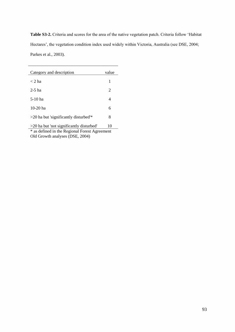
93

Table S3-2. Criteria and scores for the area of the native vegetation patch. Criteria follow ‘Habitat

Hectares’, the vegetation condition index used widely within Victoria, Australia (see DSE, 2004;

Parkes et al., 2003).

Category and description value

< 2 ha 1

2-5 ha 2

5-10 ha 4

10-20 ha 6

>20 ha but 'significantly disturbed'* 8

>20 ha but 'not significantly disturbed' 10

* as defined in the Regional Forest Agreement

Old Growth analyses (DSE, 2004)

94

Table S3-3. Criteria and scores relating to the distance to core area Criteria follow ‘Habitat Hectares’,

the vegetation condition index used widely within Victoria, Australia (see DSE, 2004; Parkes et al.,

2003). Core area is defined as an area >50 ha.

Distance Core Area not Core Area

significantly disturbed significantly disturbed

>5 km 0 0

1-5 km 2 1

<1 km 4 3

contiguous 5 4

95

Table S3-4. Estimated carrying capacities for various pasture types in south-eastern Australia (source

Blackwood et al., 2006; NSW-DPI, 2012; Saul et al., 2009, 2011)

DSE, Dry Sheep Equivalent

Pasture types Estimated range of DSE ha-1

Low quality native pasture (without management) 0.5 – 2.0

Good quality native pasture (some management

input)

1.5 – 3.0

Improved native pasture (seed and fertiliser applied) 2.0 – 5.0

Managed pasture (seed + fertiliser but not irrigated) 6.0 – 10.0

Managed irrigated pasture 10.0 – 16.0

Degraded pasture 0.25 – 0.5

96

Table S3-5. Summary of the main GIS data layers used in the analysis.

Layer name Description Data type Resolution Data source

ALUM land use

and land cover

The Australian Land Use and Management (ALUM) Classification system provides a nationally

consistent method to collect and present land use information that provides valuable information

about the reasons for change in the condition of natural resources and associated ecosystem

goods and services.

Vector N/A Australian Bureau of

Rural Sciences

Ecological

vegetation

classes (EVC)

EVCs are a type of native vegetation classification described through a combination of floristic,

life forms and ecological characteristics, and through an inferred fidelity to particular

environmental attributes.

Vector N/A Victorian Department of

Sustainability and

Environment

Plantation

database

Plantation database provides various useful details regarding managed plantations, such as, year

of planting, area, species types, previous land use which are utilised to classify age classes, patch

size and landscape context.

Vector N/A Various forestry

companies

Threatened Flora Data layer contains only Threatened flora as defined in the DSE Threatened Flora Advisory List.

This dataset is intended to be used for the determination of the distribution of threatened flora

species.

Vector N/A Victorian Department of

Sustainability and

Environment

Threatened

Fauna

Layer contains records of threatened species of wildlife from the Atlas of Victorian Wildlife. Vector N/A Victorian Department of

Sustainability and

Environment

Aerial

photographs

A high resolution and fully ortho-rectified aerial photographs of the study area used to

differentiate/correct some land use and land cover types

Raster 1:10,000 Victorian Department of

Sustainability and

Environment

Climate data Mean annual precipitation, temperature etc Table N/A Australian Bureau of

Meteorology

N/A – spatial resolution not applicable

97

References for Appendix and supporting Tables

Battaglia, M., Sands P.J., White, D., Mummery, D., 2004. CABALA: a linked carbon, water and

nitrogen model of forest growth for silvicultural decision support. For. Ecol. Manag. 193,

251‒282.

Benyon, R.G., England, J., Eastham, J., Polglase, P., White, D., 2007. Tree Water Use In Forestry

Compared To Other Dry-Land Agricultural Crops In The Victorian Context: Report prepared

for the Department of Primary Industries Victoria to promote scientific knowledge in this area;

Ensis, 2007. Technical report no. 159. Victorian Department of Primary Industries, Melbourne.

Blackwood, I., Briggs, G., Christie, J., Davies, L., Griffiths, N., 2006. Beef stocking rates and farm

size – Hunter Region, NSW Department of Primary Industries, Orange, NSW.




Bush, D., Lamb, K., Tickle, P., and Pritchard, A., 1998. Central Highlands (Victoria) plantation

potential analysis: methodology and results. Bureau of Resource Sciences, Canberra.

DPI-NSW 2012. Department of Primary Industries, New South Wales, Retrieved from

http://www.dpi.nsw.gov.au/agriculture/farm-

business/budgets/livestock/sheep/background/dse#Table2

DSE, 2004. Vegetation Quality Assessment Manual–Guidelines for applying the habitat hectares

scoring method. Version 1.3. Victorian Government Department of Sustainability and

Environment, Melbourne.

DSE, 2009. Victoria’s State of the Forest Report 2008, Victorian Government Department of

Sustainability and Environment, Melbourne.



Grierson, P.F., Adams, M.A., Attiwill, P.M., 1993. Estimates of carbon storage in the above-ground

biomass of Victoria’s forests. Aust. J. Bot. 40, 631‒640.

http://www.dpi.nsw.gov.au/agriculture/farm-business/budgets/livestock/sheep/background/dse#Table2

http://www.dpi.nsw.gov.au/agriculture/farm-business/budgets/livestock/sheep/background/dse#Table2

98

Guo, L.B., Cowie, A.L., Montagu, K.D., Gifford, R.M., 2008. Carbon and nitrogen stocks in a native

pasture and an adjacent 16-year-old Pinus radiata D. Don. plantation in Australia. Agric.

Ecosyst. Environ. 124, 205‒218.

IPCC, 2006. 2006 IPCC Guidelines for National Greenhouse Gas Inventories, Prepared by the

National Greenhouse Gas Inventories Programme, Eggleston H.S., Buendia L., Miwa K., Ngara

T. and Tanabe K. (Eds). IGES, Japan.

Norris, J., Arnold, S., Fairman, T., 2010. An indicative estimate of carbon stocks on Victoria’s

publicly managed land using the FullCAM carbon accounting model, Aust. For. 73, 209‒219

Paul, K.I., Jacobsen, K., Koul, V., Leppert, P., Smith, J., 2008. Predicting growth and sequestration of

carbon by plantations growing in regions of low-rainfall in southern Australia. For. Ecol.

Manage. 254, 205‒216.

Paul, K.I., Reeson, a., Polglase, P., Crossman, N., Freudenberger, D., Hawkins, C., 2013. Economic

and employment implications of a carbon market for integrated farm forestry and biodiverse

environmental plantings. Land Use Policy 30, 496‒506.

Parkes, D., Newell, G., Cheal, D., 2003. Assessing the quality of native vegetation: The ‘habitat

hectares’ approach. Ecol. Manage. Restor. 4, 29‒38.


Hobart.

Saul, G., Kearney, G., Borg, D., 2009. Pasture systems to improve productivity of sheep nutritive

value and persistence of resown pastures. Anim. Prod. Sci. 49, 654‒667.

Saul, G., Kearney, G., Borg, D., 2011. Pasture systems to improve productivity of sheep in south-

western Victoria 2. Animal production from ewes and lambs. Anim. Prod. Sci. 51, 982‒989.

Tallis, H.T., Ricketts T., Nelson, E., Ennaanay, D., Wolny, S., Olwero, N., Vigerstol, K., Pennington,

D., Mendoza, G., Aukema, J., Foster, J., Forrest, J., Cameron, D., Lonsdorf, E., Kennedy, C.,


URS, 2007. Australia’s Forest Industry in the Year 2020, Department of Agriculture, Fisheries and

Forestry, Canberra.

99

CHAPTER 4: GIS-BASED CLASSIFICATION, MAPPING AND VALUATION OF

ECOSYSTEM SERVICES IN PRODUCTION LANDSCAPES

This chapter has been published in a peer-reviewed conference proceedings as follows:

Baral, H., Kasel, S., Keenan, R. J., Fox, J., Stork, N., 2009. GIS-based classification, mapping and

valuation of ecosystem services in production landscapes: A case study of the Green Triangle region

of south-eastern Australia. In: Thistlethwaite, R., Lamb, D., Haines, R. (Eds.), Forestry: a Climate of

Change. Caloundra, pp. 64–71.

4.1. ABSTRACT

This paper presents a GIS-based approach for classification, mapping and valuation of selected

ecosystem services using market and non-market valuation techniques. First, we identified and

compiled a variety of spatial and non-spatial data and developed a land cover typology of the study

area into a GIS environment. Second, we estimate the annual flow of economic value of each service

using various economic valuation techniques. We found that the economic value of market ecosystem

services such as timber and carbon was relatively straightforward. However the quantification and

valuation of non-market services such as biodiversity was complicated. Finally, we produced an

annual flow of total economic value of sub-catchment G8 of the Lower Glenelg Basin, south-eastern

Australia using the spatial economic valuation technique. We expect that this work will highlight

research avenues to advance the ecosystem services framework as an operational basis in plantation

dominant production landscapes in Australia and elsewhere.

100

4.2. INTRODUCTION

Production landscapes provide a variety of benefits for human beings – such as food, fibre, flood

protection, clean water, and clean air. The benefits human populations derive, directly or indirectly,

from ecosystem functions are labelled as ecosystem services (Costanza et al. 1998). According to this

definition the goods and services are derived from the ‘functions’ and are utilised by ‘people’. The

goods and services produced by the ecosystem are not always complementary, because the production

of certain goods and services often results in the depletion or degradation of other goods and services.

For example, timber extraction can affect visual quality, water quality and recreation. However, with

proper management, there is a potential to integrate a variety of goods and services in production

landscapes. The nature and typology of ecosystem services has been extensively elaborated elsewhere

(de Groot et al. 2002; Boyd & Banzhaf 2007; Fisher & Kerry 2008; Wallace 2008; Fisher et al. 2009).

The process of identifying, classifying, quantifying and mapping ecosystem services at the landscape

level is increasingly recognised as an essential prerequisite for the efficient allocation of natural

resources (Heal et al. 2005). Estimating the economic value of ecosystem services can play an

important role in conservation planning and ecosystem-based management (Plummer 2009; Stenger et

al. 2009). Conversely, a lack of economic valuation can potentially conceal the importance of such

resources. However, economic valuation of ecosystem services requires up-to-date and reliable

information and considerably better understanding of the landscapes that provide such services (Troy

& Wilson 2006).

We present a framework for classifying and mapping ecosystem services for a production landscape

and assess the value of both market and non-market goods and services in a Geographic Information

System (GIS). This provides a baseline estimate of the ecosystem services value (ESV) of selected

ecosystem services, such as timber, carbon, water regulation and biodiversity.

101

4.3. CLASSIFICATION MAPPING AND ECONOMIC VALUATION

4.3.1. GIS AS AN ECOSYSTEM SERVICES MAPPING TOOL

Ecosystem services are not homogenous across the landscape and their supply changes through time

(Fisher et al. 2009). For this reason, ecosystem services are best expressed and most easily studied at

particular spatial and temporal scales (MEA 2003). GIS provides land managers with a tool for

quantifying and mapping the values of multiple ecosystem services across landscapes for improved

resource planning and decision planning. Moreover, the valuation of ecosystem services, and

understanding of how these resources interact, also provides an indication of trade offs and synergies.

This paper will demonstrate how GIS can be used to analyse disparate data to generate spatially

explicit results within a production landscape.

4.3.2. ECONOMIC VALUATION OF ECOSYSTEM SERVICES

The knowledge and recognition of the importance of ecosystem services in providing benefits to

society, and as the basis for the sustainable functioning of natural systems, have grown in recent

years. Despite their importance, ecosystem services are yet to be incorporated into decision making

(Chan et al. 2006). Many of these goods and services are not valued on markets and there is a gap

between market valuation and the economic value of many ecosystem services (Stenger et al. 2009).

Ecosystem goods and services can be divided into two broad categories: (i) the provision of direct

market goods or services such as timber, pulp and carbon; and (ii) the provision of non-market goods

or services, which include biodiversity and habitat for plant and animal life (Wilson & Hoehn 2006;

Mertz et al. 2007). Economic valuation of the former is straightforward while the latter is more

complicated and controversial (Wilson & Hoehn 2006; Stenger et al. 2009). However, resource

managers and policy analysts involved in protecting and managing natural resources must make

decisions which involve multiple trade-offs in allocating resources. These are mainly economic

102

decisions and based either explicitly or implicitly on the value society places on services. To this end,

economic valuation provides a useful tool for justifying set priorities and programs, policies, or

actions that protect or restore ecosystem and associated services.

4.3.3. ECOSYSTEM VALUATION TECHNIQUES

Market price method: This method estimates the economic value of ecosystem goods or services that

are bought and sold in commercial markets. This method can be used to value changes in either the

quantity or quality of a good or service (Wilson & Hoehn 2006). In this study, this method was used

to estimate the economic values of timber/pulp and carbon sequestration.

Non-market valuation methods: Values for many ecosystem goods and services are not readily

captured in market transactions, and thus require non-market valuation methods, such as travel cost

method, hedonic approach, and contingent valuation (Wilson & Hoehn 2006; Stenger et al. 2009).

4.3.4. ENVIRONMENTAL VALUE TRANSFER

Value transfer is an accepted economic methodology which obtains an estimate for the economic

value of non-market goods or services through work conducted at another site or group of sites (Troy

& Wilson 2006). The ‘transfer’ itself refers to the application of economic values and other

information from the original ‘study site’ to a ‘policy site’. This technique was used in this study to

estimate the economic value of biodiversity and associated services.

103

4.4. METHODOLOGY

4.4.1. STUDY AREA

The study location lies within the Green Triangle region of southern Australia, some 300 km west of

Melbourne, Victoria, and covers approximately 305 km2 (Fig. 4-1). The area is known as sub-

catchment G8 of the Glenelg Hopkins Catchment. This area was selected because of its concentration

of commercially valuable hardwood and softwood plantations where the focus is on production

forestry with the provision of a variety of environmental services.

The area has a variable annual rainfall of approximately 800 mm and mean annual temperature of 8

ºC (min) to 19 ºC (max). The altitudinal gradient ranges from 8–198 m above sea level. The major

land use in G8 is production forestry including both hardwood (Eucalyptus globulus) and softwood

(Pinus radiata) plantations (Refer Fig. 4-3). There are also some large areas of uncleared crown land

(reserved forest) and limited grazing of sheep and cattle. Few social networks and services are

available in sub-catchment G8 with Digby the only township, with a population of about 50 people.

Community based groups include Rifle Downs Landcare, Miakite-Grassdale Tree Group, and the

Smokey River Land Management Group.

104

Figure 4-1. Location of the study area – sub-catchment G8, Lower Glenelg Basin within The Green

Triangle region of south-eastern Australia. Shading represents areas of high to low relief according to

a digital terrain model.

4.4.2. METHODS

The approach is based on a combination of market-based and non-market valuation techniques and

has six key steps: (i) define the study area, identify the data requirement and compile data; (ii)

develop land cover typology; (iii) select ecosystem services for economic valuation; (iv) map land

cover and associated ecosystem services; (v) quantify goods and services and calculate economic

value; and (vi) assign economic value in GIS and calculate total ecosystem service value (Fig. 4-2).

105

Figure 4-2. Conceptual framework for the method of classification, mapping and economic valuation

of ecosystem services used in this study

The first step was to identify both spatial and attribute data requirements, and then compile the data

from a variety of sources. Datasets included: (i) plantation GIS data, which includes location, plant

year, species, previous land use; (ii) ecological vegetation class (EVC); (iii) location of threatened

flora and fauna; (iv) a digital terrain model; and (v) topographic data such as contours, roads and

watercourses. EVCs are systems of classifying native vegetation types based on differences in broad

landscape features and environmental regimes (DNRE, 1997). EVC and plantation statistics provide

an important overview of land cover types of the study area as vegetation is a highly visual

component of the landscape and is an important part of timber resources as well as flora and fauna

habitats. This study used the EVC dataset developed by the Victorian Department of Sustainability

and Environment, and plantation GIS data available from the forestry companies represented in the

study area (ITC, Timbercorp, Hancock Victorian Plantations, Wollybutt, Midway Afforestation, Great

Southern Plantations, Green Triangle Plantation Forests, and Auspine).

106

The second step entails development of land cover typology for the study area and starts with a

preliminary analysis of available GIS data and EVCs. Land cover types from EVC and plantation data

present in the study area are listed, a range of ecosystem services produced from each land cover type

are identified and possible means of quantification and economic valuation techniques are reviewed.

Ecosystem services identified in step two are screened in the third step in order to determine which

are most relevant to the planning and decision making, and to set priorities for further assessment and

valuation. Given the limited time and resources, it was not possible to assess in detail all the

ecosystem services and assign economic value.

In the fourth step, a land cover map is created using analysis tools in GIS which combine input layers

from the diverse data sources to produce the final land cover map. Although significant variation

within each land cover type may exist due to various factors, such as slope, aspect, and soil type, this

level of detail was not measured in this preliminary study. Once each land cover type is finalised, then

goods and services provided by each land cover type is quantified and economic value is assigned

(Step 5). The economic value of ecosystem services was summed and cross-tabulated by each good

and service and land cover type. Finally, a total spatial economic value map was produced (Step 6) by

transferring ecosystem services value calculated in Step 5 using an ArcGIS 9.2 (from ESRI Inc.). The

equation below illustrates the calculation of total ecosystem services value (ESV) in GIS environment

(Troy and Wilson 2006).

1

( ) ( )· ( )n

i i ki

k

V ES A LU V ES

……(i)

Where A(LUi) = area of land use/cover type (i), and V(ESki) = annual value per unit area of ecosystem

service type (k) generated by each land cover type (i)

107

4.4.3. ECOSYSTEM SERVICES IDENTIFIED AND VALUATION FOR THIS STUDY

Although there are large numbers of ecosystem services produced by the sub-catchment G8 (timber or

fibre, carbon sequestration and climate regulation, water regulation, biodiversity and associated

services, erosion control, salinity mitigation, tourism, recreation and cultural value), this study only

focused on four goods and services – timber, carbon, water, and biodiversity and associated services.

4.4.3.1 TIMBER

Plantation GIS data available from various forestry companies were used to identify and map the

areas for timber production. Timber yield per hectare was calculated using a generic growth model

(Fig. 4-4) available from Farm Forestry Toolbox (FFT) (Version 5.0, Private Forests Tasmania).

Current timber value per unit area was estimated by multiplying the current stumpage price for

hardwood and softwood logs and for pulpwood. Current market prices (2009 as a base year) were

reviewed from Product Disclosure Statements (PDS) issued by various Managed Forestry Investment

Scheme (MIS) forestry projects. The accuracy of growth and yield calculated from FFT was not

validated with actual growth and yield data due to high level of confidentiality of inventory data.

4.4.3.2 CARBON

A generic Carbon Sequestration Predictor (Version 3.1, New South Wales Department of Primary

Industries) was used to estimate average carbon sequestration per hectare per year. Plantation GIS

data were used to classify sites and determine the area and age of plantation. The average market

value of current CO2 trading in Australian and international markets was used to calculate carbon

value.

108


Classifying, measuring and valuing biodiversity was a challenging issue for a number of reasons – (i)

it was complicated by the wide spectrum of biotic scales at which biodiversity operates, ranging from

the molecular specific to the ecosystem level; (ii) even for a given level of diversity, e.g., presence of

certain threatened flora or fauna, there is no well established and agreed means for defining,

measuring and valuing biodiversity; and (iii) a number of different indicators have been proposed

which neither provide consistent nor comparable results on which to base general interpretations

(Bene & Doyen 2008).

As detailed mapping and valuation of biodiversity was not within the scope of this study, we were left

with two alternatives – (i) transfer biodiversity values from other studies; or (ii) use an approximate

dollar value employed by the Australian and various State government initiatives to conserve native

vegetation on private land, such as ‘bush tender’ and ‘habitat hectare’ in Victoria, ‘biodiversity

banking’ in New South Wales, ‘NatureAssist’ in Queensland, and ‘levy/biodiversity offset package’

in South Australia. The second option was used due to lack of comparable studies to transfer

appropriate values for this site. The estimated value was transferred to each land cover type of native

remnant vegetation.

4.4.3.4. WATER

Estimating accurate water use by plantations and various vegetation types is also a difficult issue. It is

generally agreed that forest plantations use such a large quantity of water that downstream flow may

be affected. Following harvest, water quantity increases but the quality may decrease where sediment

discharge in the overland flow reaches stream channels. 3-PG, a simple, process-based forest growth

model, developed by Landsberg and Waring (1997), was used estimate annual plantation water use

per unit area. The average water harvesting charge per megalitre available from the Independent

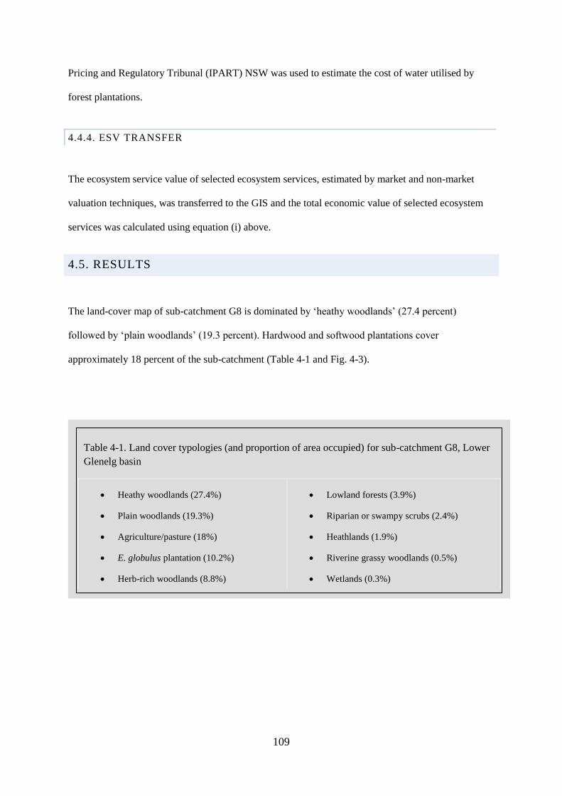
109

Pricing and Regulatory Tribunal (IPART) NSW was used to estimate the cost of water utilised by

forest plantations.

4.4.4. ESV TRANSFER

The ecosystem service value of selected ecosystem services, estimated by market and non-market

valuation techniques, was transferred to the GIS and the total economic value of selected ecosystem

services was calculated using equation (i) above.

4.5. RESULTS

The land-cover map of sub-catchment G8 is dominated by ‘heathy woodlands’ (27.4 percent)

followed by ‘plain woodlands’ (19.3 percent). Hardwood and softwood plantations cover

approximately 18 percent of the sub-catchment (Table 4-1 and Fig. 4-3).

Table 4-1. Land cover typologies (and proportion of area occupied) for sub-catchment G8, Lower

Glenelg basin

Heathy woodlands (27.4%)

Plain woodlands (19.3%)

Agriculture/pasture (18%)

E. globulus plantation (10.2%)

Herb-rich woodlands (8.8%)

P. radiata plantation (7.3%)

Lowland forests (3.9%)

Riparian or swampy scrubs (2.4%)

Heathlands (1.9%)

Riverine grassy woodlands (0.5%)

Wetlands (0.3%)

110

The values of the selected ecosystem services – timber, carbon, biodiversity and water – have

distinctly different spatial distributions, although some areas are of high value for multiple services

while others are low value (Fig. 4-5). For example, the preliminary assessment and economic

valuation of these ecosystem services indicate plantations represent the highest economic value per

unit area. This is mainly due to the relatively detailed valuation of consumptive services available

from commercial plantation areas. The areas with higher timber yields also produce more carbon

which further increases the economic value per unit area.

The value of native vegetation is relatively low due to our use of the conservation value based on

various government initiatives to conserve native vegetation in private land. This does not reflect the

true value of all native vegetation and the value of a number of other services such as erosion control

and water regulation are not assessed in this study.

The land cover map (Fig. 4-3) was based on the most recent, updated plantation and native vegetation

datasets. However, improved estimates for growth and yield, together with improved conservation

values, will permit further refinement of our valuation of ecosystem services for sub-catchment G8.

111

Figure 4-3. Land cover map of sub-catchment G8, Lower Glenelg Basin.

112

Figure 4-4. Site productivity (top) and mean annual increment (bottom) for Pinus radiata (4a, b) and Eucalyptus globulus (4c, d) used to estimate timber

yield ha-1

,(where, MDH = mean dominant height, MDDob = mean dominant diameter over bark and MAI = mean annual increment.)

113

Figure 4-5. Sum of annual flow of selected Ecosystem services of sub-catchment G8, Lower Glenelg Basin. Total flow of ESV is generated using equation (i)

the large light grey area indicates ESV less than $1350 ha-1

yr-1

or no data available at this stage.

114

4.6. DISCUSSION

The quantification and valuation of timber and carbon were relatively straightforward due to readily

available datasets. Similarly, the accuracy level is relatively high because prices are well-defined, and

real data and accepted economic techniques were used. However, some issues, such as the true

economic value of goods or services, may not be fully reflected in market transactions which are

subject to market imperfections, seasonal variations and unforeseen impacts on markets.

Other services which are not readily bought and sold in the market place, such as biodiversity and

water quantity and quality, are difficult to quantify and value. The complexity and uncertainty

underlying the functioning of biodiversity contribute to the difficulty in assessing such services (Bene

& Doyen 2008). Although it is difficult to put an accurate price tag on such services, it is important to

estimate the value of these ecosystem services because of the growing environmental market.

While the current global financial downturn threatens markets for timber resources, eco-products are

gaining in market popularity due to perceived environmental challenges, such as drought, declining

supplies of drinking water, and loss of biodiversity (Metz et al. 2007). The economic valuation of

ecosystem services provides better understanding of these forms of natural capital which is critical to

our ability to plan and manage it over long term.

The critical underlying assumption of the value transfer approach is that the economic value of

ecosystem goods or services at the study site can be inferred with sufficient accuracy from the

analysis of existing valuation studies. Clearly, as the level of information increases within the source

literature, the accuracy of the value transfer improves. For this reason we are currently compiling

recent forest ecosystem valuation studies in Australia as most existing datasets are outdated.

We are also in the process of accessing CABALA (CArbon BALAnce), a more advanced model for

predicting forest growth and carbon sequestration in plantations and managed forests developed by

CSIRO, and anticipate that tree growth and carbon estimation will improve as a result.

115

4.7. CONCLUSIONS

This study presented a simple GIS-based process of classification, mapping and valuation of

ecosystem goods and services at the landscape scale. Rather than a single methodological approach,

this study used a number of tools to estimate ESV using market and non-market based valuation

approaches in a spatially explicit manner. Although the study is still in its early stages and does not

account for all non-market ecosystem services, it demonstrates an important contribution of such

services at a landscape level. The approach and methodology can be used for more precise future

mapping for all ecosystem goods and services, including agriculture, pasture and other forest goods

and services.

116

4.8. REFERENCES

Bene, C & Doyen, L 2008, ‘Contribution values of biodiversity to ecosystem performances: A

viability perspective’, Ecological Economics, 68 (1‒2), 14‒23.

Boyd, J & Banzhaf, S 2007, ‘What are ecosystem services? The need for standardized environmental

accounting units’, Ecological Economics, 63 (2‒3), 616‒626.

Chan, KMA, Shaw, M, Cameron, DR, Underwood, E & Daily, G 2006, ‘Conservation Planning for

Ecosystem Services’, Plos Biology, 4 (11), e379.

Costanza, R, d’Arge, R, de Groot, R, Farber, S, Grasso, M, Hannon, B, Limburg, K, Naeem, S,

O’Neill, RV, Paruelo, J, Raskin, RG, Sutton, P & van den Belt, M 1998, ‘The value of

ecosystem services: putting the issues in perspective’, Ecological Economics, 25 (1), 67‒72.

de Groot, RS, Wilson, MA & Boumans, RMJ 2002, ‘A typology for the classification, description and

valuation of ecosystem functions, goods and services’, Ecological Economics, 41 (3), 393‒408.

DNRE 1997, Victoria’s Biodiversity: Directions in Management, Department of Natural Resources

and Environment, East Melbourne.

Fisher, B & Kerry, T 2008, ‘Ecosystem services: Classification for valuation’, Biological

Conservation, 141 (5), 1167‒1169.

Fisher, B, Turner, RK & Morling, P 2009, ‘Defining and classifying ecosystem services for decision

making’, Ecological Economics, 68 (3), 643‒653.

Heal, GM, Barbier, EB & Boyle, KJ 2005, Valuing Ecosystem Services: Toward Better

Environmental Decision-Making, Washington, DC.

MEA 2003, Ecosystems and Human Well-being: A framework for Assessment, Island Press,

Washington DC.

Mertz, O, Ravnborg, HM, Lovei, G, Nielsen, I & Konijendijk, CC 2007, ‘Ecosystem services and

biodiversity in developing countries’, Biodiversity and Conservation, 16 (10), 2729‒2737.

Metz, B, Davidson, O, Bosch, P, Dave, R, and Meyer, L 2007, Climate Change 2007: Mitigation of

Climate Change, Cambridge University Press, London.

117

Plummer, ML 2009, ‘Assessing benefit transfer for the valuation of ecosystem services’, Frontiers in

Ecology and the Environment, 7 (1), 38‒45.

Stenger, A, Harou, P & Navrud, S 2009, ‘Valuing environmental goods and services derived from the

forests’, Journal of Forest Economics, 15 (1), 1‒14.

Troy, A & Wilson, MA 2006, ‘Mapping ecosystem services: Practical challenges and opportunities in

linking GIS and value transfer’, Ecological Economics, 60 (2), 435‒449.

Wallace, K 2008, ‘Ecosystem services: Multiple classifications or confusion?’, Biological

Conservation, 141 (2), 353‒354.

Wilson, MA & Hoehn, JP 2006, ‘Valuing environmental goods and services using benefit transfer:

The state-of-the art and science’, Ecological Economics, 60 (2), 335‒342.

119

CHAPTER 5: SPATIAL ASSESSMENT AND MAPPING OF BIODIVERSITY AND

CONSERVATION PRIORITIES IN A HEAVILY MODIFIED AND FRAGMENTED

PRODUCTION LANDSCAPE IN NORTH-CENTRAL VICTORIA, AUSTRALIA

This chapter has been accepted for publication as follows:

Baral, H., Keenan, R.J., Sharma, S.K., Stork, N.E., Kasel, S., (accepted for publication 18 Sep. 2013).

Spatial assessment and mapping of biodiversity and conservation priorities in a heavily modified and

fragmented production landscape in north-central Victoria, Australia. Ecological Indicators.

5.1. ABSTRACT

Human impacts on the natural environment have resulted in a steady decline in biodiversity and

associated ecosystem services. A major policy and management challenge is to efficiently allocate

limited resources for nature conservation to maximize biodiversity benefits. Spatial assessment and

mapping of biodiversity value plays a vital role in identifying key areas for conservation and

establishing conservation priorities. This study measured biodiversity value using readily available

data and tools in order to identify conservation priority sites in a heavily modified and fragmented

production landscape. The study also assessed trade-offs among biodiversity and other ecosystem

services. We used spatial tools for assessing and mapping biodiversity such as Patch Analyst in

ArcGIS 10.2 to assess landscape alteration states, and the Integrated Valuation of Ecosystem Services

and Trade-offs to identify habitat quality. Results indicated that areas of high biodiversity

conservation value were concentrated in less modified land-cover types. Substantially modified land-

cover types (generally associated with agriculture and irrigated pastures) had lower habitat quality and

biodiversity value. The analysis revealed that assessments based solely on habitat condition may not

be the most suitable basis for conservation planning because this does not include associated adjacent

land uses, roads or other threats to biodiversity. Spatially targeted environmental plantings and less

intensive agroforestry that reconnect native remnants in heavily fragmented landscapes can provide

significant potential conservation outcomes. Planned landscape reconfiguration based on readily

120

available spatial data can yield net positive benefits to biodiversity by halting degradation of remnant

native vegetation and increasing total habitat area.

5.2. INTRODUCTION

In recent years, the importance of biodiversity to global economies, human welfare and survival has

been well documented and widely recognised (Butchart et al., 2010; Duffy, 2009; Rands et al., 2010;

Steffen et al., 2009; TEEB, 2009). In Australia, biodiversity continues to decline in spite of Federal

and state government efforts to manage threats (Bennett, 2003; DSE, 2010; NRMC, 2010; OECD,

2008; SoE, 2011; Steffen et al., 2009) with similar trends globally (Butchart et al., 2010; CBD, 2010;

MEA, 2005; Steffen et al., 2009). Moreover, Australia has suffered the largest documented extinction

of species of any continent over the last 200 years (DSEWPC, 2011). The main identified threats to

biodiversity in Australia include loss, fragmentation and degradation of habitat or natural ecosystems,

spread of invasive species, unsustainable use of natural resources, inappropriate fire regimes, and

climate change (Bennett, 2003; NRMC, 2010; Steffen et al., 2009).

With significant expansion in production landscapes for agricultural activity around the world and a

resultant ongoing decline of natural systems (FAO, 2005; World Bank, 2010), there is an increasing

focus on the role of production landscapes in conserving biodiversity and providing a variety of

ecosystem services (Bélair et al., 2010; Kandziora et al., 2013; Wilson et al., 2010). Securing

biodiversity in the production landscape can enhance agricultural productivity through pollination and

pest regulation, water quality and nutrient regulation, soil stabilisation, and carbon sequestration

(Hopper et al., 2005; Kasel et al., 2011; Scherr and McNeely, 2008; Tscharntke et al., 2005). While

there is ongoing debate about the relative merits of integrated versus partitioned conservation activity

(Phalan et al., 2011; Tscharntke et al., 2012), conservation policy makers and land managers are

giving strong support to conserving biodiversity in highly modified production landscapes (Wilson et

al., 2010). Spatial assessment and mapping of conditions suitable for biodiversity conservation or

restoration are also essential for the establishment of baseline biological data that will aid successful

121

conservation planning and management in highly modified landscapes (Eigenbrod et al., 2009; Jones-

Walters, 2008) and help identify priority sites for allocating limited resources (Brooks et al., 2006;

Higgins, 2006).

Extent and quality of habitat conditions are often used as proxies of biodiversity ( Nelson et al., 2011;

Tallis et al., 2010) and remote sensing based techniques are being increasingly employed to generate

biodiversity and ecosystem services indicators (García-Gómez and Maestre 2011; Lück-Vogel et al.,

2013; Nagendra et al., 2013; Spanhove et al., 2012). Recent research has focused on linking current

land use and vegetation types to biodiversity and associated ecosystem services (Burkhard et al.,

2012; Falcucci et al., 2007; Foley et al., 2005; Hector and Bachi, 2007; Kandziora et al., 2013; Yapp

et al., 2010 ). A variety of approaches have been used to identify conservation priority sites within

production landscapes, each focused on a different aspect of biodiversity (e.g., Kandziora et al., 2013;

Schneiders et al., 2012; Tallis et al., 2010) from global (Brooks et al., 2006; Jongman, 2013) to local

scale (Higgins, 2006; Jongman, 2013). Given the imperative for expeditious implementation of

conservation solutions (Watts and Handley, 2010), rapid assessment approaches that use readily

available data and tools are highly desirable (Baral et al., 2013; Burkhard et al., 2012; Grantham et al.,

2008, 2009).

The aim of this study is to spatially characterise a heavily modified and fragmented production

landscape and assess biodiversity value using readily available data and tools in order to identify

conservation priority sites. An additional aim is to assess the effect of land-use change on the

provision of biodiversity and associated ecosystem services. To achieve these objectives we used

spatial approaches and tools for biodiversity assessment and mapping such as Integrated Valuation of

Ecosystem Services and Trade-offs (InVEST) biodiversity models (Tallis et al., 2010) and patch

analyst tool (Rempel et al., 1999, 2012). The resulting data and maps and subsequent analyses are

used to consider the opportunities for re-configuring natural vegetation in cleared, modified and

degraded landscapes to meet new sustainable landscape management objectives. Furthermore, we

comment on the suitability of InVEST tools for habitat quality assessment and conservation planning.

122

5.3. METHODS

5.3.1. STUDY SITE

The study site is located in north-central Victoria, Australia between Kerang and Lake Boga,

approximately 320 km north-west of Melbourne (35.972º S, 143.228º E, Fig. 5-1). The total area

spans about 30,000 ha, essentially defined by the boundaries of the Little Murray and Lower Loddon

Rivers in the North, West and South and the Murray Valley Highway in the West. Within the study

area lies the Winlaton and Reedy Lakes Future Farming Landscapes (FFL) projects managed by

Kilter Pty Ltd. The terrain is generally flat and low-lying (70-80 m above sea level) despite being a

considerable distance from the coast. Mean annual rainfall of 50 years average is approximately 370

mm and mean annual temperature ranges from a minimum of 9 ºC to a maximum of 23 ºC.

Land and water use in the study area are dynamic. Irrigation water entitlements are being bought and

sold, and there are ongoing changes in where and how farming takes place, and with people moving

from rural properties to regional town centres (NCCMA, 2007). More recently, Kilter Pty Ltd (an

asset management group servicing the superannuation sector), has been selecting land in north-central

Victoria and managing it under Future Farming Landscapes (FFL), a long-term program that aims to

restore landscapes to their most sustainable configurations. Through this program 25% or 7552 ha of

the Reedy Lakes and Winlaton study area is currently being reconfigured and managed for both

traditional and new income streams including agriculture, forestry, green energy, and water. This

potential for future land-use change presented an ideal opportunity to assess the current status of

biodiversity and associated ecosystem services provided by each land use-land cover type as a

baseline for assessing the implications of future land management options.

123

Figure 5-1. Location of the Reedy Lakes, Winlaton study area and major land use-land cover types in

north central Victoria, Australia.

124

The area has been subject to extensive vegetation clearing for agriculture and pastoral production,

with native vegetation now highly fragmented and often degraded (NCCMA, 2005). Since European

settlement in the mid 1800s, an estimated 70% of native vegetation (18,300 ha) has been cleared.

Associated effects of this clearing include widespread declines in biodiversity, increased soil and

stream salinity and soil erosion (NCCMA, 2011). Each of these land management problems is of

national importance (Steffen et al., 2009) and for this reason this study area is reflective of the

challenges affecting many parts of the region. Major land use-land cover types and the proportion of

the area occupied by each land use in Reedy Lakes and Winlaton include: (i) irrigated farming, 28%;

(ii) dryland cropping, 26%; (iii) native vegetation, 23%; (iv) degraded land undergoing rehabilitation,

10%; (v) water, 10%; and (vi) other, 3%.

Reedy Lakes and Winlaton covers less than 0.2 % of Victoria’s land mass; however, it supports a

relatively large number of threatened flora (50 species, 2.5% of the total threatened flora for Victoria)

and fauna (81 species, 45% of the total threatened species) (DSE, 2008a, b). The high levels of

biodiversity, along with the pressures on it, have resulted in Reedy Lakes and Winlaton being

identified as an important site for conservation by the Victorian Government (DSE, 2010). Wetlands

within the study area support a high diversity and abundance of waterfowl species (Lugg et al., 1989)

and some are of international significance, including the ‘Kerang Wetlands Ramsar Site’ (Fig. 5-1).

5.3.2. GIS DATA, SOFTWARE AND ANALYTICAL TOOLS

A number of datasets were compiled for the study site from a variety of sources and stored in

Geographic Information System (GIS) database. Key datasets included: (i) a recent land use map

based on the Australian Land Use and Management (ALUM) classification (BRS, 2006) (ii) native

vegetation/Ecological Vegetation Classes (EVC) (DSE, 2011), (iii) threatened flora and fauna (DSE

2008a, b), (iv) Land Management Unit (LMU) data (Kilter Pty Ltd, 2011), (v) climate data, and (vi)

topographical data such as roads, contours and watercourses. GIS raster datasets, with a land use-land

cover code for each cell were produced by collating these datasets into ArcGIS 10.2 from ESRI Inc.

125

All datasets were projected into UTM54 South using a GDA1994 geographic coordinate system with

the raster datasets additionally re-sampled to a common spatial resolution of a 50 m grid.

5.3.2.1. PATCH ANALYST TOOL

For this study, size and distribution of landscape patches were assessed for native vegetation including

grasslands using the Patch Analyst extension for ArcGIS 10.2 (Rempel et al., 1999, 2012) and the

output used to classify the landscape into alteration classes. The distribution of remnant native

vegetation in Reedy Lakes and Winlaton was quantified using spatial metrics such as patch size and

connectivity. Remnant native vegetation was categorised into three patch sizes based on area

(Michaels et al. 2008): small patches (<10 ha), medium patches (10-50 ha) and large patches (>50 ha).

We analysed core area (Rempel et al., 1999) with application of different buffers of 25 m, 50 m, and

100 m following Michaels et al. (2008) and evaluated the number of patches in each of three patch

area categories relative to the initial patch analysis.

5.3.2.2. INVEST TOOL

The biodiversity model in InVEST tools generates two key sets of information useful in making an

initial assessment of conservation needs: the relative extent and habitat quality in a region and its

changes across time (Tallis et al., 2010). This tool assumes that large areas with a high habitat quality

would support more flora and fauna species and individuals, and the areas that decrease in habitat

extent and quality over time would contain reduced levels of biodiversity. More detailed description

of input data for InVEST are outlined in Table 5-1 and a more detailed description of calculating a

parcel’s habitat-quality and rarity score is outlined by Bai et al. (2011), Leh et al. (2013), Nelson et al.

(2011), Polasky et al. (2011), and Tallis et al. (2010).

5.3.3. LAND COVER

126

For this study we used current land use-land cover types for the InVEST analysis (Tallis et al. 2010;

Table 5-1) and a possible future land use based on proposed land use reconfiguration by the Future

Farming Landscapes program to assess the impact of land-use change on biodiversity and various

ecosystem services. The planned future land use reconfiguration covers 25% of the study area and

includes: (i) irrigated cropping, 37%; (ii) biodiversity and environmental planting, 26%; (iii) grazing,

20%; (iv) perennial horticulture, 9%; and (v) agroforestry, 5%. A large number of native tree species

are included under the environmental planting programme including Mallee Eucalypt (Eucalyptus

dumosa), Black Box (Eucalyptus largiflorens), Red Gum (Eucalyptus camaldulensis) and a variety of

Acacia species (Kilter Pty Ltd, 2011).

5.3.4. CONSERVATION PRIORITY SITES

Conservation priority sites were identified according to a number of criteria including: (i) extant

vegetation types and their bioregional conservation status within the region, (ii) biodiversity goals and

resource condition targets of the study region, and (iii) and relative abundance of threatened fauna and

flora (Table S5-1).

127

Table 5-1. Input data for InVEST biodiversity model

*LULC, Land use-land cover

Data Description

Current LULC map A GIS raster dataset with a numeric LULC code for each cell, 1 Native

vegetation, 2 Agriculture, 3 Pasture, 4 Water bodies, 5 Built up areas.

Threat data and sources A table of threats considered for this analysis e.g., agriculture, built up areas

and sealed and unsealed roads and GIS raster file of the distribution and

intensity of each threat. GIS shape files of polygons with data on the

relative degree of proximity to potential threats (roads, built-up areas and

agriculture) were used to assess the impact on biodiversity.

Accessibility to sources of

degradation

A GIS polygon shape file containing data on the relative protection which

provides barriers against threats. Formal conservation areas and protected

lands were considered sites with minimum accessibility and were assigned a

threat level of 0, while polygons with maximum accessibility (e.g. poorly

enforced ownership, extractive reserves) were assigned 1. Polygons under

intermediate levels of protection were assigned values between 0 and 1 (

Polasky et al., 2011; Tallis et al., 2010;).

Sensitivity of habitat types

to each threats

A table of LULC types whether or not they are considered habit and for

LULC types that are habitat, their specific sensitivity to each threat.

Sensitivity values range from 0 to 1 where 0 represents no sensitivity to a

threat and 1 represents the greatest sensitivity (Polasky et al., 2011).

Sensitivity scores are determined from the literature and expert knowledge

(Bai et al., 2010; Polasky et al., 2011; Tallis et al., 2010).

Half-saturation constant The numeric value indicating the half saturation constant. InVEST model

uses a half-saturation curve is used to convert habitat degradation scores to

habitat quality scores (Tallis et al., 2010). An inverse relationship between

the degradation score and its habitat quality score is determined by this half-

saturation constant. The half-saturation constant used was equal to the grid

cell degradation score that returns a pixel habitat quality score of 0.5. That

is, if the half-saturation constant is 10 then any pixel with a degradation

score of 10 will have a habitat quality score of 0.5 (Tallis et al., 2010).

128

5.3.5. LAND-USE CHANGES AND IMPACT ON BIODIVERSITY AND

ASSOCIATED ECOSYSTEM SERVICES

Key ecosystem services associated with biodiversity in the study area are listed in Table 5-2 (DSE

2004, 2010; Parks Victoria, 2000; Steffen et al., 2009). A rapid qualitative assessment of ecosystem

services provides an understanding of land use-land cover change and associated impacts on various

ecosystem services. For this study we used peer reviewed papers, published reports and expert

opinion for qualitative assessment and ranking (Baral et al., in press, Bullock et al., 2007, 2011; Cao

et al., 2009; Dowson and Smith, 2007; de Groot and van der Meer, 2010; MEA, 2005; Ostle et al.,

2009; Shelton et al., 2001; ). In addition, feedback from other stakeholders and agencies has also been

incorporated.

To assess the impacts of land use-land cover changes we used three temporal reference points – (i)

pre-European condition from modelled historical vegetation data: it was assumed that the study area

was intact native vegetation until European settlement and vegetation modification in the early 1850s,

(ii) current or intensive agricultural focus: the large proportion of native vegetation converted to

agriculture since the 1850s, and (iii) future farming landscape: proposed landscape reconfiguration

through the FFL program.

129

Table 5-2. Key ecosystem services associated with biodiversity in the Reedy Lakes and Winlaton study area. Letters in brackets represent Millennium

Ecosystem Assessment categories: provisioning (P), Regulating (R), Cultural (C) and Supporting (S) services.

Ecosystem services Description

Forage production (P) Production of forage for domestic livestock mainly from pasture and grazing land

Water supply (P) Provision of water for consumptive use, includes both quality and quantity

Carbon stock (R) Storage of carbon in wood, other biomass and soil

Carbon sequestration (R) Capture atmospheric carbon dioxide in trees, shrubs and other vegetation

Water regulation (R) Regulation of hydrological flows by vegetation and microorganisms

Salinity water disposal (R) Storage of saline water

Flood control (R) Control of floods

Nutrient regulation (R) Internal cycling, processing and acquisition of nutrients by vegetation and microorganisms

Pollination (R) Pollination of wild plant species and harvested crops

Aesthetic beauty (C) Attractive landscape features helps enjoyments of scenery

Recreation (C) Travel to natural ecosystems for eco-tourism, outdoor sport etc

Soil protection (S) Promotes agricultural productivity and the integrity of natural ecosystems

Wildlife habitat (S) Landscapes capacity to hold naturally functioning ecosystems support a diversity of plants and animal life

130

Table 5-3. Summary of native vegetation patch analysis in the Reedy Lakes and Winlaton study area.

Metric Value

Patch Density and Size Metrics

Number of Patches 4098

Mean Patch Size (ha) 1.8

Median Patch Size (ha) 0.06

Patch Size Coefficient of Variance 2036.4

Patch Size Standard deviation 35.6

Edge Metrics

Total Edge (km) 1931

Edge Density 269.4

Mean Patch Edge (m) 471.2

Shape Metrics

Mean Shape Index 1.4

Area Weighted Mean Shape Index 9.4

Mean Perimeter-Area Ratio 3008.2

Mean Patch Fractional Dimension 1.5

Area Weighted Mean Patch Fractal Dimension 1.4

Diversity and Interspersion Metrics

Shannon’s Diversity Index 4.0

Shannon’s Evenness Index 0.5

131

5.4. RESULTS

5.4.1. SPATIAL CHARACTERISATION OF THE LANDSCAPE – PATCH ANALYST

TOOL

Twenty two percent of the study area (6,800 ha) supported native vegetation. This vegetation was

highly fragmented, in more than 4,000 irregularly shaped patches. Of these patches 98.5% were small

sized patches (<10 ha), 1.2% were medium sized (10-50 ha) and only 0.3% were large sized (>50 ha).

Although there was one large block of approximately 1,800 ha intact native vegetation (Fig. 5-2), the

small sized patches of native vegetation dominated the landscape with mean patch size of 1.8 ha and

median patch size of 0.06 ha. Small sized patches of native vegetation were distributed predominantly

(82%) on privately owned land subject to agricultural and pastoral land uses. However, 40% of

medium and larger patches were located on public land, often within conservation and habitat

protection areas. Other metrics associated with native vegetation patch analysis such as, edge, shape

and diversity and interspersion metrics are presented in Table 5-3.

The extent to which patches are at risk of depletion is dependent on the size of patches and the area of

edge. This was assessed by measurement of various sized buffers (25 m, 50 m, and 100 m) around the

patch. Increasing buffer size substantially decreased the number of patches of remnant vegetation. For

example using a 25 m buffer reduced the number of vegetation patches by more than 50% (4,098 to

1,804) and a 100 m buffer, reduced the number of isolated patches by over 95%.

132

5.4.2. RELATIVE HABITAT QUALITY ACROSS THE LANDSCAPE – INVEST

TOOL

The InVEST tool indicated that a very small proportion of the landscape currently provides high

habitat quality and associated biodiversity values. Larger vegetation patches usually support greater

habitat quality (Fig. 5-3), although this depended on surrounding land use-land cover and their

associated threats. Two wildlife reserves and part of a large water body i.e., Lake Boga are classified

as relatively high quality habitats. Interestingly the eastern study area boundary along the Little

Murray River shows a higher habitat quality which is due to reduced intensity of threats and larger

areas of extant native vegetation.


Based on the North Central CMA’s regional biodiversity goals and resource condition target and the

bioregional conservation status of remnant native vegetation, the study area is classified into three

categories of remnant native vegetation patches – high (44%), moderate (49%) and low (7%). The

most cleared and underrepresented EVCs in the study bioregion, and therefore the high priority for

conservation or restoration, are Plains Savannah, Plains Woodland, Chenopod Grassland and Semi-

arid Chenopod Woodland. Moderate priority sites are represented by various EVCs such as, Lignum

Swamp, Lignum Swampy Woodland, and Woorinen Mallee. Other EVCs such as Riverine Chenopod

Woodland, Grassy Riverine Swamp and Lake Bed Herbland are reasonably well represented and

classified under low priority sites. The sites with recorded threatened fauna and threatened flora are

further classified as very high priority conservation sites (Fig. 5-4).

133

5.4.4. LAND-USE CHANGE AND IMPACT ON BIODIVERSITY AND OTHER

ECOSYSTEM SERVICES

A qualitative assessment of past and future land-use changes and their impact on biodiversity and

various ecosystem services (Fig. 5-5), indicates that prior to the 1850s the study area was covered

with intact native vegetation that supported biodiversity and supplied a wide range of ecosystem

services except agricultural commodities (Fig. 5-5a). After European settlement the majority of the

landscape was cleared (over 70%), resulting in increased agriculture production at the expense of

other ecosystem services (Fig. 5-5b). Under the FFL program the reconfigured landscape includes a

combination of biodiversity, agriculture, and grazing (Fig. 5-5c). The main land-use changes from

FFL’s planned reconfiguration and associated impacts on a number of ecosystem services (Table 5-2)

is summarised in Table 5-4 which indicates an overall positive impact on a number of ecosystem

services for environmental planting, agroforestry and extensive grazing. However, there is strong

trade-off between forage and food production in the case of conversion to agriculture.

134

Figure 5-2. Distribution of native vegetation patches in Reedy Lakes and Winlaton according to patch size. Areas currently being converted to biodiversity

planting as a part of Future Farming Landscapes are highlighted as are examples of landscape alteration states states (a1) intact, (a2) variegated, (a3)

fragmented, and (a4) relictual (after McIntyre and Hobbs, 1999), (b) extant native vegetation, (c) pre-European (1750) vegetation distribution (colours

represent simplified native vegetation groups, see Table S5-2).

135

Figure 5-3. The InVEST model of relative habitat quality.

136

Figure 5-4. Conservation priority sites based on bioregional conservation status and north-central

regional biodiversity goal and resource condition target, and sites with recorded threatened fauna and

flora.

137

Figure 5-5. Typical land-use transition in the Reedy Lakes and Winlaton study area and potential trade-offs among multiple ecosystem services: (a) pre-

1850s, (b) 1850s to current, and (c) future landscape under the Future Farming Landscapes (FFL) program. The provision of ecosystem services is applicable

to particular transitions and indicative only (figure inspired by Foley et al., 2005).

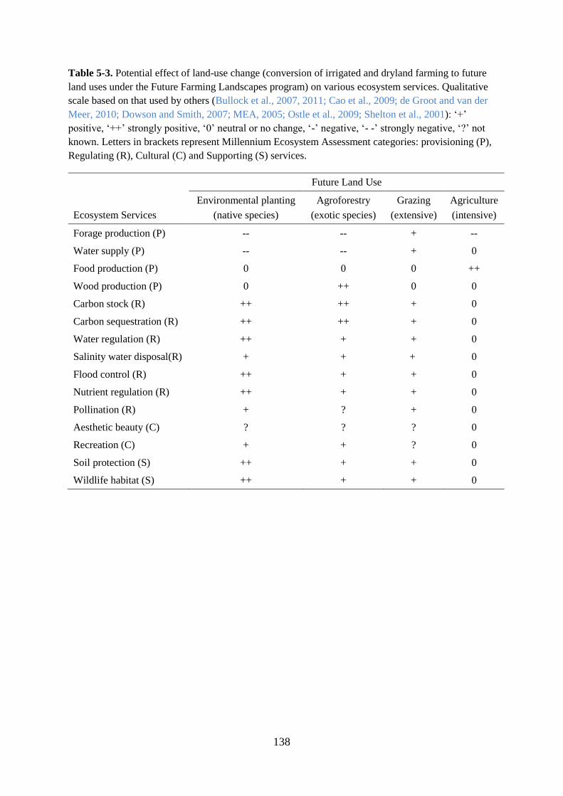
138

Table 5-3. Potential effect of land-use change (conversion of irrigated and dryland farming to future

land uses under the Future Farming Landscapes program) on various ecosystem services. Qualitative

scale based on that used by others (Bullock et al., 2007, 2011; Cao et al., 2009; de Groot and van der

Meer, 2010; Dowson and Smith, 2007; MEA, 2005; Ostle et al., 2009; Shelton et al., 2001): ‘+’

positive, ‘++’ strongly positive, ‘0’ neutral or no change, ‘-’ negative, ‘- -’ strongly negative, ‘?’ not

known. Letters in brackets represent Millennium Ecosystem Assessment categories: provisioning (P),

Regulating (R), Cultural (C) and Supporting (S) services.

Future Land Use

Ecosystem Services

Environmental planting

(native species)

Agroforestry

(exotic species)

Grazing

(extensive)

Agriculture

(intensive)

Forage production (P) -- -- + --

Water supply (P) -- -- + 0

Food production (P) 0 0 0 ++

Wood production (P) 0 ++ 0 0

Carbon stock (R) ++ ++ + 0

Carbon sequestration (R) ++ ++ + 0

Water regulation (R) ++ + + 0

Salinity water disposal(R) + + + 0

Flood control (R) ++ + + 0

Nutrient regulation (R) ++ + + 0

Pollination (R) + ? + 0

Aesthetic beauty (C) ? ? ? 0

Recreation (C) + + ? 0

Soil protection (S) ++ + + 0

Wildlife habitat (S) ++ + + 0

139

5.5. DISCUSSION

This study demonstrates that readily available spatial datasets and tools can be used to assess habitat

quality and biodiversity values in human-dominated landscapes and can be useful for initial

assessment and conservation planning. Our analysis also indicates that there is a high potential for

protecting and enlarging small remnant patches for reducing fragmentation and increasing

connectivity and associated biodiversity at the landscape scale.

5.5.1. SPATIAL CHARACTERISATION OF THE LANDSCAPE – PATCH ANALYST

TOOL

Results from native vegetation patch analysis provided a wide range of indices relevant to landscape

alteration state and opportunities for reconnecting landscapes for biodiversity enhancement in the

study area. Michaels et al. (2008) assessed the level of landscape modification in north-west Tasmania

based on the extent and distribution of remnant native vegetation. Similar to this study, their results

suggest that conserving small remnants patches and revegetating around them can enhance landscape

connectivity by reducing fragmentation at the landscape scale. However, parts of the study area were

in a relictual state with limited capacity to be restored (McIntyre and Hobbs, 1999). In many cases,

fragmented remnant vegetation may contribute some biodiversity value, including their role as

stepping stones for biodiversity to move to larger patches and as dispersal sources (Lindenmayer and

Fischer, 2006; Michaels et al., 2008; Rubio and Saura, 2012). Hilty et al. (2006) proposed planting

corridors of native vegetation as a solution to habitat fragmentation allowing species to move between

isolated fragments. Others have suggested that such appropriately located biodiversity corridors may

be important in allowing plant and animal species to migrate due to climate change (Baranyi et al.,

2011). Such corridor plantings need to start with the protection and connection of relatively high

value biodiversity patches (CEF, 2012). If remnant native vegetation is to be managed sustainably on

heavily modified agricultural land, its role in providing other ecosystem services, such as carbon

140

storage or water quality, needs to be assessed, and in turn can support, and provide funding for

conservation (CEF, 2012; Crossman et al., 2011; Foley et al., 2005).

5.5.2. RELATIVE HABITAT QUALITY ACROSS THE LANDSCAPE – INVEST

TOOL

Vegetation condition assessment and mapping has become a major priority for Australian agencies

and organizations responsible for natural resource management (Pert et al., 2012). However current

approaches used in various Australian states , the ‘habitat hectares approach’ in Victoria (Parkes et al.,

2003), ‘biometric approach’ in New South Wales (Gibbons et al., 2008), and ‘bio-condition mapping’

in Queensland (Eyre et al., 2011) focus mainly on vegetation condition with limited consideration of

surrounding landscape and potential threats, and may not lead to the best biodiversity conservation

decisions. The results of the InVEST tool differ to those of the Victorian government Department of

Sustainability of Environment for the same area (Newell et al., 2006), and indicates that a focus solely

on vegetation condition without considering surrounding landscape context and potential threats may

not lead to the best biodiversity conservation decisions. Patterns in biodiversity habitat quality are

inherently spatial and should be analysed in conjunction with the surrounding threats (Paukert et al.,

2011) and their relative impact, the sensitivity of habitat to each threat, and distances between the

habitats and sources of threats (Pert et al., 2012; Tallis et al., 2010).

Our results indicate that different assessment approaches might yield quite different results, impacting

on conservation and restoration investment choices. However, there is a positive relationship between

the size of native vegetation patch and habitat quality – that was consistent with many other studies

(Fischer et al., 2006; Munro et al., 2007; Newell et al., 2006). This is especially true in fragmented

production landscapes where a number of threatening processes surround remnant native vegetation

and where smaller patches are more susceptible than larger patches (Munro et al., 2007). To this end,

conservation measures should focus on consolidating smaller vegetation patches in to larger blocks.

Landscape scale biodiversity assessments need to include the whole mosaic of land cover and land

141

uses, including small fragments or individuals in areas used for pastoral production or agriculture

outside patches of native vegetation.


In recent years, there has been some progress towards biodiversity conservation, with an additional

2,000 ha of habitat improved for biodiversity conservation and the risk of extinction reduced for

threatened flora and fauna at priority sites (NCCMA, 2011). However the study area still has a low

cover of native vegetation (<30% of pre-European) and is therefore a high priority for protection of

remaining EVCs based on the regional biodiversity goal and resource condition targets (NCCMA,

2003, Table S1). The location of biodiversity and associated threats are distributed unevenly therefore

it is essential to prioritise the area for conservation to minimise the loss (Brooks et al., 2006; Higgins,

2006). Conservation priority maps generated in this study (Fig. 5-4) provide an indicative guide to

natural resource managers and investors of where to allocate the limited resources available for nature

conservation in order to maximize biodiversity benefits (Higgins, 2006). However, distribution of

records of threatened fauna and flora are concentrated near water-bodies and accessible sites. This is

mainly due to issues surrounding accessibility and the use of water bodies for recreational purposes by

those people reporting species occurrences. Consequently, they may present a biased picture of habitat

requirements, particularly for fauna.

In areas of high priority sites, conservation organisations can partner with other stakeholders

interested in a variety of services to effect outcomes, effectively increasing the resources available for

conservation (Goldman et al., 2008) and maximise the return on conservation investment (Underwood

et al., 2008).

142

5.5.4. LAND-USE CHANGES AND PROVISION OF BIODIVERSITY AND

ECOSYSTEM SERVICES

The relationship between biodiversity values and the provision of ecosystem services has been

extensively discussed (Hectar and Bagchi, 2007; Kandziora et al., 2013; Kareiva et al., 2011; Leadely

et al., 2010; Turner et al., 2007). Ecosystems functions affected by loss of biodiversity include

pollination, seed dispersal, climate regulation, carbon sequestration, and agricultural pest and disease

control (MEA, 2005). This is particularly important in this study area, where ecosystem services such

as water quality, soil conservation and pollination are economically important. Provision of ecosystem

services further justifies conservation and restoration of native vegetation (CEF, 2012; Nelson et al.,

2008). Conservation purely for the sake of biodiversity is difficult to justify without first

demonstrating direct benefits to human beings (Chen et al., 2010).

Land management has a major impact on biodiversity and the provision of ecosystem services. In

many parts of the world, land-use change has altered most of the landscape and resulted in substantial

ecological consequences such as decline in biodiversity and ecosystem services (Zhao et al., 2006).

Our study landscape has undergone considerable habitat loss and fragmentation in a relatively short

history of European occupation. We found that the proposed land-use changes in this study landscape

could result in a net positive gain to biodiversity, mainly due to conversion of intensively-managed

agriculture and pasture land to environmental plantings, low intensity grazing and agroforestry

activities. The InVEST results inferred that smaller, fragmented patches that are exposed to threats are

generally of low conservation value. Smaller patches may sustain smaller populations which increases

the probability of extinction resulting from environmental and demographic pressures (Fischer and

Lindenmayer, 2007). Therefore biodiversity plantings and other revegetation work will be more

effective if they are consolidated to existing remnant vegetation patches in order to create larger

habitat patches that have a higher probability of being randomly occupied by a given individual or

species than smaller patches (Connor and McCoy, 1979). This confirms the view of McIntyre and

Hobbs (1999) that relictual landscapes are of lower priority for conservation investments. The data

143

from this study provides a basis for reconfiguring and consolidating the current biodiversity

investment program for greater conservation benefits.

Limitations of applying geo-spatial and remote sensing techniques including InVEST tools for

biodiversity assessments include the lack of assessment of small-scale characteristics and finer details

(Spanhove et al., 2012) and field verification is required in many cases (Hernández-Stefanoni et al.,

2011; Lück-Vogel et al. 2013). Furthermore, the value of a patch of habitat for species or ecosystem

will depend on size, quality, functional condition, surrounding land uses and suitability for rare or

threatened species. While the basic biodiversity model of the InVEST tool takes surrounding land

uses into consideration, the habitat value of a patch is limited to its size.

5.6. CONCLUSIONS

Conservation of biodiversity and associated ecosystem services in highly modified and fragmented

production landscapes is a crucial natural resource management issue in Australia and elsewhere.

Availability of data and appropriate tools are often identified as issues in assessment of biodiversity

and ecosystem services. Here we successfully demonstrate spatial approaches to classifying the

landscape for habitat quality, based on the size, density, distribution and condition of native remnant

vegetation in the landscape scale. Our findings indicate that simple and readily available spatial data,

tools and models can be useful for conservation assessment, planning and management and, as

observed by Polasky et al. (2008), higher levels of both biodiversity conservation and the provision of

ecosystem services can be achieved by appropriate spatial patterns of restoration activities.

Conservation organisations, or catchment management bodies, businesses and individual landowners

can use these tools to align their strategies and locate their restoration activities on priority sites to

maximize the outcomes of their conservation investment (Kareiva, 2010; Underwood et al., 2008).

144

5.7. REFERENCES

Baral, H., Keenan, R.J., Fox, J.C., Stork, N.E., Kasel, S., 2013. Spatial assessment of ecosystem

goods and services in complex production landscapes: A case study from south-eastern

Australia. Ecological Complexity 13, 35–45.

Baral, H., Keenan, R.J., Stork, N.E., Kasel, S., in press. Measuring and managing ecosystem goods

and services in changing landscapes: a south-east Australian perspective. J. Environ. Plann.

Manage. DOI: 10.1080/09640568.2013.824872

Bai, Y., Zhuang, C., Ouyang, Z., Zheng, H., Jiang, B., 2011. Spatial characteristics between

biodiversity and ecosystem services in a human-dominated watershed. Ecol. Complex. 8, 177–

183.

Baranyi, G., Saura, S., Podani, J., Jordán, F., 2011. Contribution of habitat patches to network

connectivity: Redundancy and uniqueness of topological indices. Ecol. Indic. 11, 1301–1310.

Bélair, C., Ichikawa, K.L., Wong, B.Y., Mulongoy, K.J., 2010. Sustainable use of biological diversity

in socio-ecological production landscapes. Background to the ‘Satoyama Initiative for the

benefit of biodiversity and human well-being, Secretariat of the Convention on Biological

Diversity, Montreal.

Bennett, J., 2003. The economic value of biodiversity: a scoping paper. Paper presented to the

national workshop The Economic Value of Biodiversity, 22–23 October 2003.

Brooks, T.M., Mittermeier, R.A., Da Fonseca, G.A.B., Gerlach, J., Hoffmann, M., Lamoreux, J.F.,

Mittermeier, C.G., Pilgrim, J.D., Rodrigues, A.S.L., 2006. Global Biodiversity Conservation

Priorities. Science 313, 58–61.

145




Bullock, J.M., Aronson, J., Newton, A.C., Pywell, R.F., Rey-Benayas, J.M., 2011. Restoration of

ecosystem services and biodiversity: conflicts and opportunities. Trends Ecol. Evol. 26, 541–

549.

Bullock, J.M., Pywell, R.F.,Walker, K.J., 2007. Long-term enhancement of agricultural production by

restoration of biodiversity. J. Appl. Ecol. 44, 6–12


budgets. Ecol. Indic. 21, 17–29.

Butchart, S.H., Walpole, M., Collen, B., van Strien, A., Scharlemann, J.P., Almond, R.E., Baillie J.E.,

Bomhard, B., Brown, C., Bruno, J., Carpenter, K.E., Carr, G.M., Chanson, J, Chenery, A.M.,

Csirke, J., Davidson, N.C., Dentener, F., Foster, M., Galli, A., Galloway, J.N., Genovesi, P.,

Gregory, R.D., Hockings, M., Kapos, V., Lamarque, J.F., Leverington, F., Loh, J., McGeoch,

M. A., McRae, L., Minasyan, A., Hernández, Morcillo, M., Oldfield, T.E., Pauly, D., Quader,

S., Revenga, C., Sauer J.R., Skolnik, B., Spear, D., Stanwell-Smith, D., Stuart, S.N., Symes, A.,

Tierney, M., Tyrrell, T.D., Vié, J.C., Watson, R., 2010. Global biodiversity: indicators of recent

declines. Science 328(5982), 1164–1168.

Cao, S., Chen, L., Yu, X., 2009. Impact of China’s Grain for Green Project on the landscape of

vulnerable arid and semi-arid agricultural regions: A case study in northern Shaanxi Province. J

Appl. Ecol. 46, 536–543.

CBD, 2010. Global biodiversity outlook 3: executive summary. Secretariat of the Convention on

Biological Diversity, Montréal.

CEF, 2012. Biodiversity fund fact sheet. Clean Energy Future, Australian Government, Canberra.

146

Chen, X., Lupi, F., Viña, A., He, G., Liu, J., 2010. Using cost-effective targeting to enhance the

efficiency of conservation investments in payments for ecosystem services. Conserv. Biol. 24,

1469–1178.

Connor, E. F., McCoy, E. D., 1979. The statistics and biology of the species-area relationship. Am.

Nat. 113:791–833.

Crossman, N.D., Bryan, B. A, Summers, D.M., 2011. Carbon payments and low-cost conservation.

Conserv. Biol. 25, 835–45.

de Groot, R.S., van der Meer, P.J., 2010. Quantifying and valuing goods and services provided by

plantation forests. In: Bauhus, J., Meer, P. van der, Kanninen, M. (Eds.), Ecosystem Goods and

Services from Plantation Forests. Earthscan, London, pp. 16–42.

Dawson, J.J.C, Smith, P., 2007. Carbon losses from soil and its consequences for land-use

management. Sci. Total Environ. 382, 165–190.

DSE, 2004. Kerang Lakes Ramsar Site Strategic Management Plan, Department of Sustainability and

Environment, East Melbourne, Victoria.

DSE, 2008a. Threatened fauna 100 (GIS databases), biodiversity policy and programs, Department of

Sustainability and Environment, East Melbourne, Victoria.

DSE, 2008b. Threatened flora 100 (GIS databases), biodiversity policy and programs, Department of


DSE, 2010. Kerang Wetlands Ramsar site ecological character description, Department of




147

DSEWPC, 2011. Biodiversity Conservation. Department of Sustainability, Environment, Water,

Populations and Community. Canberra, ACT.

Duffy, J.E., 2009. Why biodiversity is important to the functioning of real-world ecosystems. Front.

Ecol. Environ. 7, 437–444.

Eigenbrod, F., Anderson, B.J., Armsworth, P.R., Heinemeyer, A., Jackson, S.F., Parnell, M., Thomas,

C.D., Gaston, K.J., 2009. Ecosystem service benefits of contrasting conservation strategies in a

human-dominated region. Proc. R. Soc. Biol. Sci. 276 (1669), 2903–2911.

Eyre, T.J., Kelly, A.L., Neldner, V.J., 2011. Method for the Establishment and Survey of Reference

Sites for BioCondition Version 2.0. Department of Environment and Resource Management

(DERM), Biodiversity and Ecological Sciences Unit, Brisbane.

Falcucci, A., Maiorano, L., Boitani, L., 2007. Changes in land-use/land-cover patterns in Italy and

their implications for biodiversity conservation. Landsc. Ecol. 22, 617–631.

FAO, 2005. Global Forest Resource Assessment, FAO Forestry Paper 147, Rome.

Fischer, J., Lindenmayer, D. B., 2007. Landscape modification and habitat fragmentation: a synthesis.

Global Ecol. Biogeogr. 16:265–280.

Fischer, J., Lindenmayer, D.B., Manning, A.D., 2006. Biodiversity, ecosystem function, and

resilience: ten guiding principles for commodity production landscapes. Front. Ecol. Environ. 4,

80–86.

Foley, J.A., DeFries, R., Asner, G.P., Barford, C., Bonan, G., Carpenter, S.R., Chapin, F.S., Coe,

M.T., Daily, G.C., Gibbs, H.K., Helkowski, J.H., Holloway, T., Howard, E.A., Kucharik, C.J.,

Monfreda, C., Patz, J.A., Prentice, I.C., Ramankutty, N., Snyder, P.K., 2005. Global

consequences of land use. Science 309, 570–574.

García-Gómez, M., Maestre, F.T., 2011. Remote sensing data predict indicators of soil functioning in

semi-arid steppes, central Spain. Ecol. Indic. 11, 1476–1481.

148

Gibbons, P., Ayers, D., Seddon, J., Doyle, S., Briggs, S., 2008. Biometric, Version 2.0. A Terrestrial

Biodiversity Assessment Tool for the NSW Property Vegetation Plan Developer – Operational

Manual. NSW Department of Environment and Climate Change, Sydney.

Goldman, R.L., Tallis, H., Kareiva, P. Daily, G.C., 2008. Field evidence that ecosystem service

projects support biodiversity and diversify options. Proc. Natl. Acad. Sci. U.S.A. 105, 9445–

9448.



1, 190–198.

Grantham, H.S., Wilson, K. A., Moilanen, A., Rebelo, T., Possingham, H.P., 2009. Delaying

conservation actions for improved knowledge: how long should we wait? Ecol. Lett. 12, 293–

301.

Hector, A., Bachi, R., 2007. Biodiversity and ecosystem multifunctionality, Nature 448: 188–190.

Hernández-Stefanoni, J.L., Alberto Gallardo-Cruz, J., Meave, J. A., Dupuy, J.M., 2011. Combining

geostatistical models and remotely sensed data to improve tropical tree richness mapping. Ecol.

Indic. 11, 1046–1056.

Higgins, I., 2006. Vegetation condition mapping and catchment management: The North Central

Victorian experience. Ecol. Manage. Restor. 7, S68–S71.

Hilty J.A., Lidicker Jr. W.Z., Merenlender, A.M., 2006. Corridor Ecology: The Science and Practice

of Linking Landscapes for Biodiversity Conservation. Island Press, Washington, DC.

Hooper, D.U, Chapin, F.S., Ewel, J.J., Hector, A., Inchausti, P., Lavorel, S., Lawton, J.H., Lodge,

D.M., Loreau, M., Naeem, S., Schmid, B., Setälä, H., Symstad, A.J., Vandermeer, J., Wardle,

D.A., 2005. Effects of biodiversity on ecosystem functioning: a consensus of current

knowledge. Ecol. Monogr. 75, 3–35.

149

Jones-Walters, L., 2008. Biodiversity in Multifunctional landscapes, J. Nat. Conserv. 16, 117–119.

Jongman, R.H.G., 2013. Biodiversity observation from local to global. Ecol. Indic. 33, 1–4.

Kandziora, M., Burkhard, B., Müller, F., 2013. Interactions of ecosystem properties, ecosystem

integrity and ecosystem service indicators—A theoretical matrix exercise. Ecol. Indic. 28, 54–

78.

Kareiva, P., 2010. Conservation science: Trade-in to trade-up. Nature 466, 322–323.

Kareiva, P., Tallis, H., Ricketts, T.H., Daily, G.C., Polasky, S., 2011. Natural capital: theory and

practice of mapping ecosystem services. Oxford University Press, Oxford.

Kasel, S., Singh, S., Sanders, G.J., Bennett, L.T., 2011. Species-specific effects of native trees on soil

organic carbon in biodiverse plantings across north-central Victoria, Australia. Geoderma 161,

95–106.

Kilter Pty Ltd 2011. Land Management Unit (LMU) databases, Google Earth file and associated

spreadsheets. Kilter Pty Ltd., Bendigo, Victoria.

Leadley, P., Pereira, H.M., Alkemade, R., Fernandez-Manjarrés, J.F., Proença, V., Scharlemann, J.

P.W., Walpole, M., 2010, Biodiversity Scenarios: Projections of 21st century change in

biodiversity and associated ecosystem services. 132 pp. Global Biodiversity, Secretariat of the

Convention on Biological Diversity, Montreal.

Leh, M.D.K., Matlock, M.D., Cummings, E.C., Nalley, L.L., 2013. Quantifying and mapping multiple

ecosystem services change in West Africa. Agric. Ecosyst. Environ. 165, 6–18.

Lindenmayer, D.B., Fischer, J., 2006. Habitat Fragmentation and Landscape Change: An Ecological

and Conservation Synthesis. CSIRO Publishing, Melbourne, Victoria.

Lück-Vogel, M., O’Farrell, P.J., Roberts, W., 2013. Remote sensing based ecosystem state assessment

in the Sandveld Region, South Africa. Ecol. Indic. 33, 60–70.

150

Lugg, A., Heron, S., Fleming, G., O’Donnell, T., 1989. Conservation Value of Wetlands in the

Kerang Lakes Area. Report to the Kerang Lakes Area Working Group. Report No. 1

Department of Forests, Conservation and Lands, Bendigo.

McIntyre, S., Hobbs, R., 1999. A Framework for Conceptualizing Human Effects on Research

Models. Conserv.Biol.13, 1282–1292.

Michaels, K., Lacey, M., Norton, T., Jann, W., 2008. Vegetation Futures for Tasmania. In: Vegetation

Futures. Australia’s national vegetation conference, 20–22 Oct 2008, Toowoomba.

MEA, 2005. Ecosystems and human well-being: Synthesis. Millennium Ecosystem Assessment.

Island Press, Washington, DC.

Munro, N.T., Lindenmayer, D.B., Fischer, J., 2007. Faunal response to revegetation in agricultural

areas of Australia: A review. Ecol. Manage. Restor. 8, 199–207.

Nagendra, H., Lucas, R., Honrado, J.P., Jongman, R.H.G., Tarantino, C., Adamo, M., Mairota, P.,

2013. Remote sensing for conservation monitoring: Assessing protected areas, habitat extent,

habitat condition, species diversity, and threats. Ecol. Indic. 33, 45–59.

NRMC, 2010. Australia’s Biodiversity Conservation Strategy 2010–2030. Natural Resource

Management Ministerial Council, Australian Government, Department of Sustainability,

Environment, Water, Population and Communities, Canberra.

NCCMA, 2003. North Central Regional Catchment Strategy 2003–2007. North Central Catchment

Management Authority, Huntly, Victoria.

NCCMA, 2005. North Central native vegetation plan, North Central Catchment Management

Authority, Huntly, Victoria.

NCCMA, 2007. Loddon Campaspe Irrigation Region Land and Water Management Plan Summary,

North Central Catchment Management Authority, Huntly, Victoria.

151

NCCMA, 2011. Annual Report 2010–11, North Central Catchment Management Authority, Huntly,

Victoria.

Nelson, E., Cameron, D.R., Regetz, J., Polasky, S., Daily, G., 2011. Terrestrial biodiversity. In:

Natural Capital. Theory and Practice of Mapping Ecosystem Services, (Eds.) Karieva, P.,

Tallis, H., Ricketts, T.H., Daily, G.C., Polasky, S. Oxford University Press, Oxford, pp 34–50.

Nelson, E., Polasky, S., Lewis, D.J., Plantinga, A.J., Lonsdorf, A., White, D., Bael, D., Lawler, J.J.,

2008. Efficiency of incentives to jointly increase carbon sequestration and species conservation

on a landscape. Proc. Natl. Acad. Sci. U.S.A. 105, 9471–9476.

Newell, G.R., White, M.D., Griffioen, P., Conroy, M., 2006. Vegetation condition mapping at a

landscape-scale across Victoria. Ecol. Manage. Restor. 7, S65–S68.

Ostle, N.J., Levy, P.E., Evans, C.D., Smith, P., 2009. UK land use and soil carbon sequestration. Land

Use Policy 26, S274–S283.

OECD, 2008. OECD Environmental Outlook to 2030. Organization for Economic Co-operation and

Development, Paris.

Parks Victoria, 2000. Strategic Directions Statement for Victoria’s Ramsar Sites. Parks Victoria,

Melbourne.

Parkes, D., Newell, G., Cheal, D., 2003. Assessing the quality of native vegetation: The ‘habitat

hectares’approach Ecol. Manage. Resto. 4, 29–38.

Paukert, C.P., Pitts, K.L., Whittier, J.B., Olden, J.D., 2011. Development and assessment of a

landscape-scale ecological threat index for the Lower Colorado River Basin. Ecol. Indic. 11,

304–310.

Pert, P.L., Butler, J.R.A., Bruce, C., Metcalfe, D., 2012. A composite threat indicator approach to

monitor vegetation condition in the Wet Tropics, Queensland, Australia. Ecol. Indic. 18, 191–

199.

152

Phalan, B., Onial, M., Balmford, A., Green, R.E., 2011. Reconciling food production and biodiversity

conservation: land sharing and land sparing compared. Science 333, 1289–1291.

Polasky, S., Calderone, G., Duarte, T., Goldstein, J., Hannahs, N., Ricketts, T., Tallis, H., 2011.

Putting ecosystem service models to work: conservation, management, and trade-offs, in:

Kareiva, P., Tallis, H., Ricketts, T.H., Daily, G.C., Polasky, S. (Eds.), Natural Capital : Theory

and Practice of Mapping Ecosystem Services. Oxford University Press, Oxford.

Polasky, S., Nelson, E., Camm, J., Csuti, B., Fackler, P., Lonsdorf, E., Montgomery, C., White, D.,

Arthur, J., Garberyonts, B., 2008. Where to put things? Spatial land management to sustain

biodiversity and economic returns. Biol. Conserv. 141, 1505–1524.

Rands, M.R.W., Adams, W.M., Bennun, L., Butchart, S.H.M., Clements, A., Coomes, D., Entwistle,

A., Hodge, I., Kapos, V., Scharlemann, J.P.W., Sutherland, W.J., Vira, B., 2010. Biodiversity

Conservation: Challenges Beyond 2010. Science 329, 1298–1303.

Rempel, R.S., Carr, A., Elkie, P., 1999. Patch Analyst and Patch Analyst (grid) function reference.

Centre for Northern Forest Ecosystem Research, Ontario Ministry of Natural Resources,

Lakehead University, Thunder Bay, Ontario.

Rempel, R.S., D. Kaukinen., D., Carr, A.P., 2012. Patch Analyst and Patch Grid. Ontario Ministry of

Natural Resources. Centre for Northern Forest Ecosystem Research, Thunder Bay, Ontario.

Rubio, L., Saura, S., 2012. Assessing the importance of individual habitat patches as irreplaceable

connecting elements: An analysis of simulated and real landscape data. Ecol. Complex. 11, 28–

37.

Scherr, S.J., McNeely, J.A., 2008. Biodiversity conservation and agricultural sustainability: towards a

new paradigm of “ecoagriculture” landscapes. Philos. Trans. R. Soc. Lond. B Biol. Sci. 363,

477–494.

153

Schneiders, A., Van Daele, T., Van Landuyt, W., Van Reeth, W., 2012. Biodiversity and ecosystem

services: Complementary approaches for ecosystem management? Ecol. Indic. 21, 123–133.

Shelton, D., Cork, S., Binning, C., Parry, R., Hairsine, P., Vertessy, R., 2001. Application of an

ecosystem services inventory approach to the Goulburn Broken Catchment. In: Third

Australian Stream Management Conference. pp. 157–162, Brisbane.

SoE, 2011. Australia state of the environment 2011. Independent report to the Australian Government

Minister for sustainability, environment, water, population and communities. Canberra.

Spanhove, T., Vanden Borre, J., Delalieux, S., Haest, B., Paelinckx, D., 2012. Can remote sensing

estimate fine-scale quality indicators of natural habitats? Ecol. Indic. 18, 403–412.

Steffen, W., Burbidge, A.A., Hughes, L., Kitching, R., Lindenmayer, D., Musgrave, W., Smith, M.S.,

Werner, P.A., 2009. Australia’s Biodiversity and Climate Change. CSIRO Publishing,

Melbourne.

Tallis, H.T., Ricketts, T., Nelson, E., Ennaanay, D., Wolny, S., Olwero, N., Vigerstol, K., Pennington,

D., Mendoza, G., Aukema, J., Foster, J., Forrest, J., Cameron, D., Lonsdorf, E., Kennedy, C.


TEEB, 2009. TEEB for National and International Policy Makers. Summary: Responding to the

Value of Nature. United Nations Environment Programme, Geneva.

Tscharntke, T., Klein, A.M., Kruess, A., Steffan-Dewenter, I., Thies, C., 2005. Landscape

perspectives on agricultural intensification and biodiversity – ecosystem service management.

Ecol. Lett. 8, 857–874.

Tscharntke, T., Clough, Y., Wanger, T.C., Jackson, L., Motzke, I., Perfecto, I., Vandermeer, J.,

Whitbread, A., 2012. Global food security, biodiversity conservation and the future of

agricultural intensification. Biol. Conserv. 151, 53–59.

154

Turner, W.R., Brandon, K., Brooks, T.M., Costanza, R., da Fonseca, G.A.B., Portela, R., 2007. Global

Conservation of Biodiversity and Ecosystem Services. BioScience, 57, 868–873.

Underwood, E.C., Shaw, M.R., Wilson, K.A., Kareiva, P., Klausmeyer, K.R., McBride, M.F., Bode,

M., Morrison, S.A., Hoekstra, J.M., Possingham, H.P., 2008. Protecting biodiversity when

money matters: maximizing return on investment. PLoS ONE 3, 7.

Watts, K., Handley, P., 2010. Developing a functional connectivity indicator to detect change in

fragmented landscapes. Ecol. Indic. 10, 552–557.

Wilson, K.A., Meijaard, E., Drummond, S., Grantham, H.S., Boitani, L., Catullo, G., Christie, L.,

Dennis, R., Dutton, I., Falcucci, A., Maiorano, L., Possingham, H.P., Rondinini, C., Turner,

W.R., Venter, O., Watts, M., 2010. Conserving biodiversity in production landscapes, Ecol.

Appl. 206, 1721–1732.

Windle, J., Rolfe, J., McCosker, J., Lingard, A., 2009. A conservation auction for landscape linkage in

the southern Desert Uplands, Queensland. Rangeland J. 31, 127–135.

World Bank, 2010. Rising Global Interest in Farmland, World Bank Report, Washington D.C.

Yapp, G., Walker, J., Thackway, R. 2010. Linking vegetation type and condition to ecosystem goods

and services. Ecol. Complex. 7, 292–301.

Zhao, S., Peng, C., Jiang, H., Tian, D., Lei, X., Zhou, X., 2006. Land use change in Asia and the

ecological consequences. Ecol. Res. 21, 890–896.

155

Table S5-1. Biodiversity goals and resource condition targets of the study region (NCCMA, 2003).

Goal Resource condition targets

The ecological function of indigenous vegetation

communities will be maintained and, where

possible native plant and animal species will be

restored to viable levels

Target 1: Improve the quality and coverage of

all vulnerable or endangered Ecological

Vegetation Classes and any others with less than

15% (as measured by habitat hectares, Parkes et

al., 2003) by 2013

Threatened vegetation communities will increase

in extent and improve in quality to achieve net

gain by:

increasing the native vegetation cover of

the region to 30%

increasing the cover of all Ecological

Vegetation Classes to at least 15% of

their pre-1750 distribution

Target 2: Increase native vegetation coverage to

20% of the region by 2030

Target 3: Maintain and improve existing viable

population of significant threatened species from

2003

Target 4: No further bioregional extinctions

from 2003

156

Table S5-2. Original and recent (2006) extent of Ecological Vegetation Classes in the Reedy Lakes

and Winlaton study area and their bioregional conservation status (DSE, 2011).

Ecological Vegetation Class

Pre-1750

(ha)

Present 2006

(ha)

%

Remaining

Bioregional

Conservation

Status

Riverine Grassy Woodland 41 32 77 Vulnerable

Lake Bed Herbland 185 121 65 Depleted

Lignum Swamp 340 202 60 Vulnerable

Grassy Riverine Forest 9 5 56 Depleted

Lignum Swampy Woodland 5457 2387 44 Vulnerable

Grassy Riverine/Swamp

Complex 1111 460 41 Depleted

Riverine Chenopod Woodland 11323 3279 29 Depleted

Woorinen Mallee 34 9 26 Vulnerable

Chenopod Grassland 4567 787 17 Endangered

Plains Savannah 27 4 15 Endangered

Semi-arid Woodland 358 37 10 Endangered

Semi-arid Chenopod

Woodland 3547 348 10 Endangered

Plains Woodland 1 0 14 Endangered

Ridged Plains Mallee 6 0 7 Endangered

Total 27005 7671 34

157

CHAPTER 6: ECONOMIC EVALUATION OF LANDSCAPE MANAGEMENT

SCENARIOS IN NORTH-CENTRAL VICTORIA,

This chapter is being submitted to Land Use Policy:

Baral, H., Keenan, R.J., Sharma, S.K., Stork, N.E., Kasel, S., (in revision). Economic evaluation of

landscape management scenarios in north-central Victoria, Australia. Land Use Policy

6.1. ABSTRACT

Human-induced changes in the natural environment are affecting the provision of ecosystem goods

and services (EGS). The overall impact on human welfare is difficult to assess because many EGS are

not captured in economic analyses, and the distribution of economic impacts of the reduced supply of

services is not well understood. Land use plans rarely include the value of public ecosystem goods

such as climate regulation and biodiversity due to difficulties in valuing these services. In this study,

we assessed total economic value (expressed as Net Present Value, NPV, over a 30 year period) for

two types of products (agricultural commodities and timber) and three ecosystem services (carbon,

water and biodiversity) under five future land-use scenarios using varying levels of costs, prices and

discount rates. Results indicated that at higher discount rates normally applied to commercial

activities, and assuming the current prices for goods and services, NPV was highest for landscape

management scenarios aimed at maximising agricultural production. Potential income from services

such as carbon and biodiversity does not offset projected income from agriculture. At higher discount

rates, NPV was negative for the two scenarios aimed at enhancing the longer term ecological

sustainability of the landscape. These results indicate that income from carbon sequestration and

biodiversity conservation would need to be considerably higher than current levels in order to justify

focusing management of this landscape on ecological outcomes. At lower discount rates (at levels

normally associated with public investments), the more ecologically appropriate ‘mosaic farming

system’ had the highest NPV, indicating that this type of system might be attractive for investors

158

interested in longer term return horizons or wider public benefits. Higher income from carbon or

biodiversity, or increased return from timber by using higher value tree species, could potentially

make more ecologically appropriate systems profitable at higher discount rates.

This study showed that an EGS framework can be used to assess and value different land-use options

and demonstrated the potential to manage landscapes to produce a mix of EGS. This can provide a

useful input for land use policy and land management decisions.

6.2. INTRODUCTION

Human life depends on a wide variety of ecosystem goods and services (EGS) provided by healthy

ecosystems. As described in the Millennium Ecosystem Assessment (MEA), these include the

provisioning of resources such as food, fibre, and raw materials; regulating services such as water

filtration, storm buffering, and climate stabilisation; supporting services such as soil formation,

photosynthesis, and pollination; and cultural services that are spiritual, aesthetic, and recreational

services (MEA, 2005). Many human activities impede ecosystem functions, thereby reducing or

increasing flows of these EGS. While the supply of some goods is increasing, the MEA estimates

60% of the ecosystem services have declined globally in the past 50 years (MEA, 2005). However,

the critical ways in which ecosystems support and enable human well-being are rarely captured in

cost-benefit analysis for policy formulation and land use decision-making (Daily et al., 2009; Laurans

et al., 2013; Nelson et al., 2008). Recent studies highlight the need to assess trade-offs among EGS

under a variety of future land-use scenarios (Butler et al., in press; Carpenter et al., 2009; Sanon et al.,

2012; Willeman et al., 2012).

Prioritising landscapes for the production or harvest of a single ecosystem commodity, such as food or

fibre, can diminish other services such as water quality, erosion prevention or soil formation (Bennett

et al., 2010; Bryan and Crossman, 2008; Raudsepp-Hearne et al., 2010; Stoate et al., 2009), as well as

159

undermining overall ecosystem resilience (MEA, 2005). This is certainly the case for south-eastern

Australia where such trade-offs have been observed over the past two hundred years (Bryan et al.,

2010, 2011; Crossman et al., 2009, 2010; Sandhu et al., 2012). Several authors explore the spatial

patterns of provision of multiple EGS in production landscapes, focusing on the win-win

opportunities for conservation and production of multiple EGS (Bennett et al., 2009; Egoh et al.,

2008; Naidoo et al., 2008; Nelson et al., 2009; Tallis and Polasky, 2009). However only a few deal

with the economic valuation of future landscape management scenarios and associated impact on

provision of EGS.

Changes in land use and land cover are ongoing due to changes in environmental conditions, patterns

of human settlement, modes of production, and demands of society (Verburg et al., 2009). Large areas

of native vegetation in Australia have been converted to agricultural production (SOE, 2011) resulting

in unforeseen economic impacts such as the costs associated with reduced flood control, the provision

of potable water, or increased salinity and soil erosion (i.e., ecosystem services) (SOE, 2011) that are

not captured in standard analysis of farming systems. EGS research is relatively new and

quantification and valuation of services remain highly uncertain (Hou et al., in press; Johnson et al.,

2012). There are additional uncertainties with the future provision of services due to continuing land-

use change and climate change. Therefore, a gross estimate of EGS at a point in time without

considering future land-use scenarios will have limited value for decision makers (Fürst et al., in

press; Swetnam et al., 2011).

Identifying such potential changes in land cover, and measuring and managing multiple EGS under

future land-use scenarios is a key challenge for policy makers. In the state of Victoria, Australia,

efforts are underway to address these challenges. One such initiative is the Future Farming

Landscapes (FFL) program, a long-term (~ 30 years) program that aims to reconfigure landscapes to

their most sustainable use. Here, we attempt to identify and assess provision of various EGS under a

range of plausible landscape configurations, including one FFL-type scenario in this landscape.

160

Our specific aims were to (i) identify and define plausible land-use scenarios for the study area, (ii)

estimate the value of key EGS: carbon sequestration, agricultural production, water, biodiversity and

timber production under these land-use scenarios, and (iii) analyse the potential trade-offs and

synergies among multiple EGS under these land-use scenarios.

6.3. METHODS

6.3.1 STUDY AREA AND POLICY CONTEXT

The study area is located in north-central Victoria (Fig. 6-1), a region spanning over three million

hectares and encompassing three bioregions (Murray Fans, Victorian Riverina, Murray Mallee; DSE,

2004). These bioregions support over 2,000 native plant species, including 130 state-wide threatened

species with 52 of these considered to be nationally threatened (NCCMA, 2011). They also support

more than 400 native vertebrate fauna species including 101 threatened species of which 13 are

nationally threatened (NCCMA, 2011). The region has been heavily modified since European

settlement with native vegetation cleared originally for pastoral development (1860s to 1950s) and

then for cropping from the 1950s onwards (Ransom, 2011). Conversion of deep rooted perennial

vegetation to annual crops has resulted in a suite of environmental impacts including dryland salinity,

habitat and biodiversity loss, and soil degradation (Jones et al., 2007; Pittock et al., 2012). Moreover,

this region is situated within the Murray-Darling Basin – the largest river catchment area in Australia,

and clearing for crops and over-use of irrigation in this catchment has resulted in extensive

environmental impacts (CSIRO, 2012). In recent years, the Australian and state governments,

business and landowners have employed a number of strategies, including market-based instruments

for conservation, aimed at reversing this decline in environmental condition (Burgin, 2008;

Eigenraam et al., 2006).

161

6.3.2. STUDY SITE - REEDY LAKES AND WINLATON

The study site lies between Kerang and Lake Boga in north-central Victoria, Australia, approximately

320 km north-west of Melbourne (35.972º S, 143.228º E, Fig. 6-1). The total area is approximately

30,000 ha, bounded by the Little Murray and Lower Loddon Rivers in the North, West and South and

the Murray Valley Highway to the West. Within the study area lie the Reedy Lakes and Winlaton

Future Farming Landscapes (FFL) projects managed by Kilter Pty Ltd (an asset management group

servicing the superannuation sector). The terrain is generally flat and low-lying (70‒80 m above sea

level). Average annual rainfall is approximately 370 mm (mean, 1962–2012), and mean annual

temperature ranges from a minimum of 9 ºC to a maximum of 23 ºC.

Reedy Lakes and Winlaton is a typical north-central Victorian landscape that has been subject to

extensive vegetation clearing for agriculture and pastoral production and native vegetation is now

highly fragmented and often degraded (NCCMA, 2005). Since European settlement in the mid-1800s,

an estimated 70% of native vegetation (18,300 ha) has been cleared. This has resulted in widespread

declines in biodiversity, increased soil and stream salinity and soil erosion (NCCMA, 2011).

Nationally, natural resource management programs have focused on reduction in salinity, improving

water quality and environmental flows, and protecting biodiversity (Hajkowicz, 2009). Major land

use-land cover types include irrigated farming, dryland cropping, native vegetation, degraded land

undergoing rehabilitation, and water bodies (Table 6-1).

The study area covers less than 0.2 % of Victoria’s land mass. However, it supports a relatively large

number of threatened flora species (50 species, 2.5% of threatened plants in Victoria) and fauna

species (81 species, 45% of the threatened Victoria). The high levels of biodiversity, and the pressures

on this biodiversity, have resulted in the area being identified as an important site for conservation by

the Victorian Government (Wetlands Scientific Committee, 1993). Wetlands within the study area

support high richness and abundance of waterfowl species (Lugg et al., 1989) and some sites are of

international significance, including the ‘Kerang Wetlands Ramsar Site’ (DSE, 2004).

162

Figure 6-1. Location of the Reedy Lakes / Winlaton study area and major land use-land cover types

in north-central Victoria, Australia.

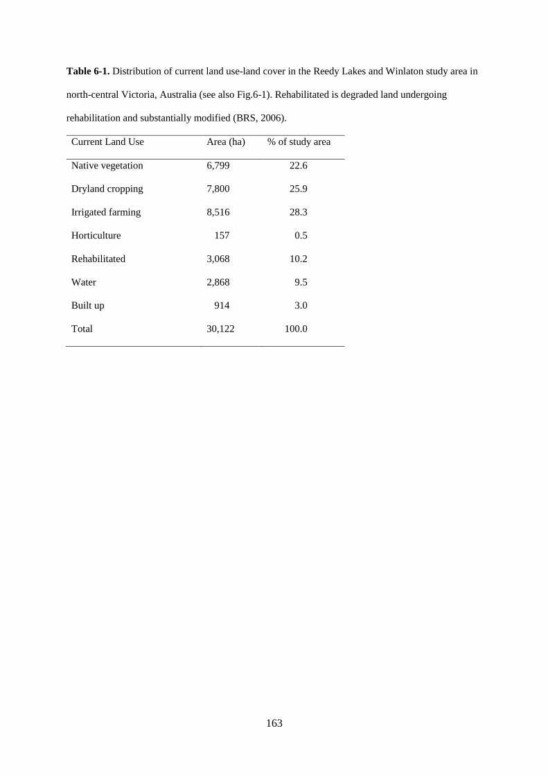
163

Table 6-1. Distribution of current land use-land cover in the Reedy Lakes and Winlaton study area in

north-central Victoria, Australia (see also Fig.6-1). Rehabilitated is degraded land undergoing

rehabilitation and substantially modified (BRS, 2006).

Current Land Use Area (ha) % of study area

Native vegetation 6,799 22.6

Dryland cropping 7,800 25.9

Irrigated farming 8,516 28.3

Horticulture 157 0.5

Rehabilitated 3,068 10.2

Water 2,868 9.5

Built up 914 3.0

Total 30,122 100.0

164

6.3.3. PLAUSIBLE FUTURE SCENARIOS FOR LANDSCAPE CONFIGURATION

AND ASSOCIATED LAND USE-LAND COVER

We developed five plausible future land-use scenarios for the study area (Table 6-2). This was based

on a review of recent land use-land cover change patterns in south-eastern Australia and undertaken in

consultation with stakeholders.

6.3.3.1. SCENARIO 1: BUSINESS-AS-USUAL (BAU)

This scenario assumed continuation of current farming and management systems with no further

broad-scale clearing of remnant native vegetation. Gradual loss of remnant vegetation and

opportunistic agricultural expansion will potentially occur at the farm scale but this was not included

in the scenario. The BAU scenario was considered plausible as the current prices of agricultural

commodities, while variable, are likely to be maintained or increased (Ransom, 2011). To this end,

farms were likely to continue operating for the foreseeable future. Under this scenario we assumed

approximately 0.14% loss of native vegetation per annum which is similar to current native vegetation

clearance rate in Victoria (DSE, 2012).

165

Table 6-2. Estimated areas of different land use-land cover under future land-use scenarios.

Descriptions of scenarios: ‘BAU’ business-as-usual, continuation of current farming and management

system; ‘MFS’ mosaic farming systems, landscape reconfiguration to more ecologically sustainable

uses that involve changes to farming practices and environmental plantings; ‘ECO’ eco-centric,

substantial increase in environmental plantings due to increasing environmental market; ‘AGRO’

agro-centric, increase in agricultural land due to higher demand of food and livestock production in

line with the population growth; ‘ALU’ abandoned land use, decline in agriculture and land

abandonment due to reduced water availability and depopulation in rural areas. In many cases, ALU

may ultimately become some form of native or exotic vegetation in the long run which may support

biodiversity. This land type may also be subject to weed and pest infestations which negatively impact

native biodiversity.

Estimated area (ha) under each scenario

Current BAU MFS ECO AGRO ALU

Native vegetation 6,799 6,519 6,799 6,799 2,297 6,799

Dryland cropping 7,800 8,079 3,900 0 10,951 0

rrigated farming 8,516 8,516 7,664 8,516 9,866 0

Horticulture 157 157 1,009 157 157 0

Freshwater lakes 2,573 2,573 2,573 2,573 2,573 2,573

Saline lakes and treatment 1,530 1,530 1,530 1,530 1,530 1,530

Channel/aqueduct 293 293 293 293 293 0

Rehabilitation 1,541 1,541 1,541 1,541 1,541 1,541

Built up 914 914 914 914 914 914

Environmental plantings 0 0 2,730 5,460 0 0

Forestry (production) 0 0 1,170 2,340 0 0

Abandoned land 0 0 0 0 0 16,765

Total 30,122 30,122 30,122 30,122 30,122 30,122

166

6.3.3.2. SCENARIO 2: MOSAIC FARMING SYSTEMS (MFS)

This scenario assumed that the landscape will be transformed to more ecologically sustainable uses

involving changes to farming practices, low rainfall forestry and environmental plantings. This

scenario is based on the FFL model and uses a similar land-use reconfiguration, with the goal of

developing an estate that includes environmental plantings and extensive grazing (~51%), irrigated

farming (horticulture, agriculture ~33%), perennial horticulture (~7%), commercial agroforestry

(~4%) and other land uses (~5%) (Kilter Pty Ltd, 2011). The MFS scenario is considered plausible

given that Kilter’s initiatives were already underway on approximately 25% of the study area (Table

3). Under this scenario we assumed that approximately 50% of dryland farming was primarily

converted to environmental planting (60% of converted land) due to the potential demand for carbon

credits, and production forestry (30% of converted land). A small proportion (10%) of irrigated

farming was assumed to be converted to perennial horticulture.

6.3.3.3. SCENARIO 3: ECO-CENTRIC OR ENVIRONMENTAL PLANTINGS (ECO)

This scenario assumed that there will be substantial increase in environmental plantings due to

growing environmental concerns and growth of new commodities based on environmental values

such as carbon and biodiversity credits (Bekessy and Wintle, 2008; Burgin, 2008). The Australian

Government and Victorian State Governments have designed economic instruments that provide

financial incentives to landowners for undertaking eligible carbon sequestration activity such as

revegetation of fragmented landscape via various mechanisms such as Carbon Farming Initiative

(DCCEE, 2011a) and the Land and Biodiversity Fund (Caripis et al., 2012; Keenan et al., 2012).

Under this scenario it was assumed that all dryland faming would be converted to mixed species

environmental planting (70%) due to potentially higher demands for carbon credits, and to a lesser

extent commercial tree farming (30%) due to low profitability.

167

6.3.3.4. SCENARIO 4: AGRO-CENTRIC OR PRODUCTION ORIENTED (AGRO)

This scenario assumed that higher demand for food and livestock production due to continued

population growth in Australia and globally (Godfray et al., 2010). Global food demand is expected to

more than double by 2050 to meet this growing demand (Green et al., 2005). Relatively cheaper land

prices, and improved farming and irrigation practices may reduce the production cost and make

agricultural production a more profitable venture. The scenario assumed the current areas of

agricultural production would increase through clearance of remnant native vegetation and conversion

to agricultural production. Under this scenario it was assumed that all available native vegetation on

private land (4,502 ha) would be cleared for dryland farming (70% of converted land) and irrigated

cropping (30% of converted land).

6.3.3.5. SCENARIO 5: ABANDONED LAND USE (ALU)

This scenario assumed that higher labour prices and a strong currency may prevent Australian

products competing effectively in international markets and reduced water availability due to water

trading and climate change, resulting in a decline in agricultural terms of trade, and agricultural land

abandonment (Garnaut, 2008; Race et al., 2010).. Under this scenario, all irrigated and dryland

farming areas would be abandoned and either revert to native vegetation or become weed infested or a

combination of both.

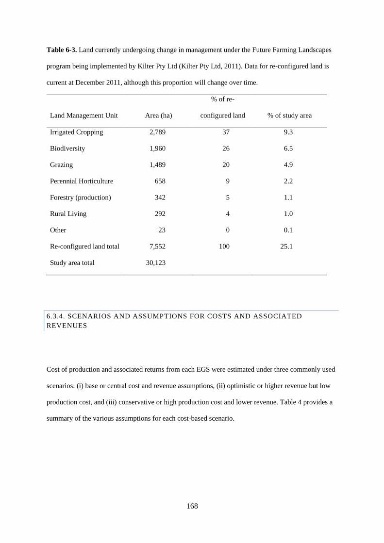
168

Table 6-3. Land currently undergoing change in management under the Future Farming Landscapes

program being implemented by Kilter Pty Ltd (Kilter Pty Ltd, 2011). Data for re-configured land is

current at December 2011, although this proportion will change over time.

Land Management Unit Area (ha)

% of re-

configured land % of study area

Irrigated Cropping 2,789 37 9.3

Biodiversity 1,960 26 6.5

Grazing 1,489 20 4.9

Perennial Horticulture 658 9 2.2

Forestry (production) 342 5 1.1

Rural Living 292 4 1.0

Other 23 0 0.1

Re-configured land total 7,552 100 25.1

Study area total 30,123

6.3.4. SCENARIOS AND ASSUMPTIONS FOR COSTS AND ASSOCIATED

REVENUES

Cost of production and associated returns from each EGS were estimated under three commonly used

scenarios: (i) base or central cost and revenue assumptions, (ii) optimistic or higher revenue but low

production cost, and (iii) conservative or high production cost and lower revenue. Table 4 provides a

summary of the various assumptions for each cost-based scenario.

169

6.3.4.1. BASE OR CENTRAL SCENARIO

This scenario used the actual establishment and management cost provided by Kilter Pty Ltd and a

carbon price of $20 Mg-1

CO2e. This price was based on the current price under the Australian

Government’s Carbon Pricing Mechanism (Clean Energy Future, 2012) less the estimated cost for

assessment and verification, which was assumed to be approximately 15% of total value. Similarly it

assumed moderate stumpage value of timber and average gross revenue from agricultural production.

6.3.4.2. OPTIMISTIC SCENARIO

This scenario used reduced establishment and annual management costs (to 50%) and a higher carbon

price $30 Mg-1

CO2e. Similarly it assumed higher stumpage value of timber and higher gross revenue

from agricultural production.

6.3.4.3. CONSERVATIVE SCENARIO

This scenario used a higher planting and annual management cost but a lower carbon price of $10 Mg-

1 CO2

e. This was an average price in the voluntary carbon market used in a number of analyses

(Crossman et al., 2011; Polglase et al., 2011). The price of agricultural commodities and livestock

would be reduced due to globalisation and increased production capacity through technological

advancements. Similarly, this conservative scenario assumed there would be a lower stumpage price

of timber and lower gross revenue from agricultural production.

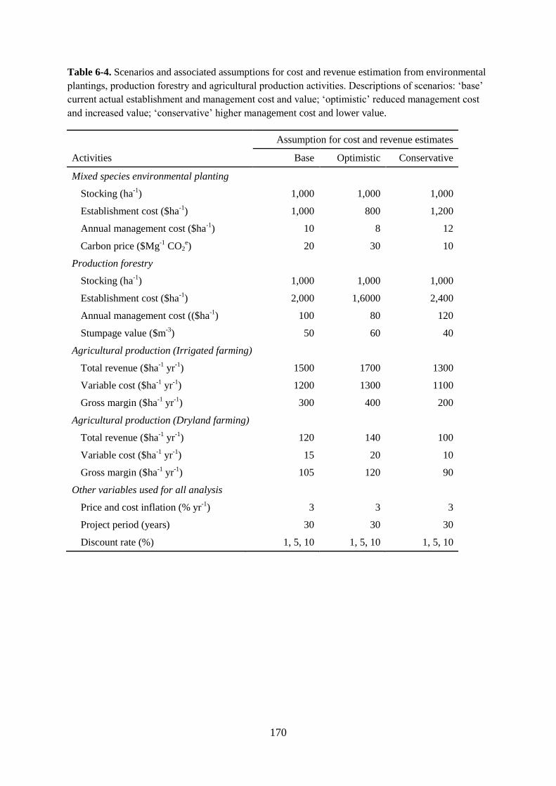
170

Table 6-4. Scenarios and associated assumptions for cost and revenue estimation from environmental

plantings, production forestry and agricultural production activities. Descriptions of scenarios: ‘base’

current actual establishment and management cost and value; ‘optimistic’ reduced management cost

and increased value; ‘conservative’ higher management cost and lower value.

Activities

Assumption for cost and revenue estimates

Base Optimistic Conservative

Mixed species environmental planting

Stocking (ha-1

) 1,000 1,000 1,000

Establishment cost ($ha-1

) 1,000 800 1,200

Annual management cost ($ha-1

) 10 8 12

Carbon price ($Mg-1

CO2e) 20 30 10

Production forestry

Stocking (ha-1

) 1,000 1,000 1,000

Establishment cost ($ha-1

) 2,000 1,6000 2,400

Annual management cost (($ha-1

) 100 80 120

Stumpage value ($m-3

) 50 60 40

Agricultural production (Irrigated farming)

Total revenue ($ha-1

yr-1

) 1500 1700 1300

Variable cost ($ha-1

yr-1

) 1200 1300 1100

Gross margin ($ha-1

yr-1

) 300 400 200

Agricultural production (Dryland farming)

Total revenue ($ha-1

yr-1

) 120 140 100

Variable cost ($ha-1

yr-1

) 15 20 10

Gross margin ($ha-1

yr-1

) 105 120 90

Other variables used for all analysis

Price and cost inflation (% yr-1

) 3 3 3

Project period (years) 30 30 30

Discount rate (%) 1, 5, 10 1, 5, 10 1, 5, 10

171

6.3.5. ECOSYSTEM GOODS AND SERVICES

We assessed and valued five important EGS provided by production landscapes using a mixed

approach of quantitative assessment and economic valuation (Butler et al., in press; Crossman et al.,

2009) for the various future land-use scenarios (Table 6-2). There are other valuable services

generated in the Reedy Lakes and Winlaton region such as, salinity mitigation, water regulation,

nutrient regulation, and recreation, but these were not considered in the analysis.

EGS values for carbon, timber, water, agricultural production and additional values from biodiversity

were estimated as net present value (NPV) per hectare over a time horizon of 30 years (t = 30) at

discount rates (r) of 1, 5, and 10%. These estimated values were compared with the estimated annual

values of agricultural production per hectare available from Kilter Pty Ltd.

6.3.5.1. CARBON SEQUESTRATION

Carbon sequestration in environmental plantings was estimated as Mg ha-1

using the Carbon Farming

Initiative (CFI) reforestation tool (DCCEE, 2011c). Monetary values were obtained firstly by

transforming Mg of C (carbon) ha-1

into Mg of CO2 ha-1

and secondly by multiplying the resulting Mg

by the assumed carbon price. Similar to Crossman et al. (2010), NPV (ha-1

) from carbon is estimated

by the following formula:

Where P is the price of carbon, Qt is the quantity of CO2e sequestrated in year t, ECc is the

establishment cost, MC is the annual management cost, and r is the discount rate.

Different carbon prices were used for base, optimistic and conservative scenarios (Table 4). For the

base scenario we used the 2012 carbon price of $23 Mg-1

of CO2 which was introduced by the

Australian Government on 1 July 2012.

172

6.3.5.2. PROVISION OF WATER

Woody vegetation usually uses a large proportion of rainfall compared to other land uses such as

agriculture and pasture and can reduce the supply of this resource in streams and rivers (Zhang et al.,

1999, 2001). Water yield from different forms of land cover was assessed based on the potential

groundwater recharge (in mm yr-1

) under given rainfall conditions (Benyon et al., 2007, 2009). Run-

off is typically estimated as the balance of water available after rain-based deep drainage and

evapotranspiration are subtracted from precipitation (Barratt et al., 2007), that is: R = P – E – D.

Here, R is run-off, P is precipitation, E is total evapotranspiration, and D is deep drainage/recharge.

However, the net change in catchment water storage over a long period of time is zero (Bradford et

al., 2001) and hence there is negligible change in deep drainage. To this end we used a simple water

balance equation following Chan et al. (2006): R = P – E.

The amount of run-off reduction from revegetation was multiplied by the cost of water per ML ha-1

to

identify the plantation water use cost for environmental planting and timber production. In the case of

irrigation, the irrigation requirement for water ML ha-1

was multiplied by the prevailing water cost in

$ ML-1

. Further details regarding water use and costs are outlined in Appendix A.


Biodiversity can be valued by society for its intrinsic worth or for its contribution to the provision of

various EGS in the study area. Both natural and modified ecosystems support certain levels of

biodiversity and a number of recent studies have focused on measuring and valuing biodiversity

(Atkinson et al., 2012; Butler et al., in press; Christie et al., 2006; Gracia et al., 2011; Salles, 2011).

However, measuring and valuing biodiversity is a challenging issue for a number of reasons: (i) it is

complicated by the wide spectrum of spatial scales at which biodiversity operates, ranging from the

molecular, to gene, species, ecosystem and landscape levels; (ii) even for a given level of biodiversity,

173

there is no well-established and agreed means for defining, measuring and valuing biodiversity; and

(iii) a number of different indicators have been proposed which neither provide consistent nor

comparable results on which to base general interpretations (Atkinson et al., 2012; Bene and Doyen,

2008; von Haaren et al., 2012).

Detailed assessment and valuation of biodiversity was not possible in this study. Rather we chose to

use an approximate dollar value for biodiversity conservation resulting from market-based approaches

used by the Australian and various State governments to conserve native vegetation on private land,

such as ‘bush tender’ in Victoria (Stoneham et al., 2003), and ‘biodiversity banking’ in New South

Wales (DECCW, 2009). This option was used because there were no comparable studies to transfer

appropriate values for the study site. The assumption was that governments would be the primary

purchasers of biodiversity conservation services from private landowners in the near future and the

recent payments for establishment of mixed species environmental plantings that increase total habitat

area and buffer existing remnant vegetation were used in the study (approximately $450 ha-1

over the

first 5 years).

6.3.5.4. TIMBER PRODUCTION

Commercial timber and wood fibre production is an ecosystem good provided by native vegetation

and managed plantations. In contrast to the declining trends for most EGS, timber production capacity

is enhanced in many parts of the world (MEA, 2005) due to increasing establishment of managed

plantations (FAO, 2010). Although the actual value of timber is realised at the time of maturity, we

converted future value in terms of net present value using various discount rates. In this study we used

the tree-stand growth model 3-PG (physiological principles predicting growth; Landsberg and

Waring, 1997) available from Farm Forestry Toolbox (Private Forest Tasmania, 2011) to estimate

timber production. The 3-PG model uses climatic data, site factors, initial tree density, and

management practices such as thinning and fertilizer application. We simulated the annual growth of

Oil Mallee (Eucalyptus kochii, a low rainfall species native to Western Australia and suitable for our

174

study site) as a monoculture plantation. Estimated mean annual increment is then multiplied with the

rotation age and various stumpage prices (S. Dawkins, Oil Mallee Australia pers. comm.) and

discount rate to calculate the net present value from timber production.

6.3.5.5. AGRICULTURAL PRODUCTION

Dryland cropping (barley, wheat, canola, oats), intensively irrigated cropping (legumes, corn,

lucerne), annual horticulture (tomatoes, melons), and perennial horticulture (olives, almonds, stone

fruits) are the dominant land use and primary economic activity in the study area (Kilter Pty Ltd,

2011). Agriculture is generally a profitable endeavour generating private returns to landowners.

However, agricultural returns are highly variable, and subject to both unpredictable weather patterns

and fluctuations in commodity markets (Ransom, 2011). The production value of agricultural land can

be quantified by (i) spatially modelling agricultural profitability according to land and water use

(Crossman et al., 2010), or (ii) obtaining estimated returns from secondary sources such as data from

Australian Bureau of Statistics or landowners and stakeholders from the particular study area. Here

we obtained present gross value of agricultural production $ha-1

yr-1

from Kilter Pty Ltd as this is

more accurate rather than extracting other sources or profitability models.

Agricultural production also contributes substantially to Australia’s total greenhouse gas emission

profile (DCCEE, 2012) but these emissions were not considered in this analysis. However, the

emissions from inputs into agricultural enterprises have to be deducted from agricultural profitability.

Here we used total estimated greenhouse gas emission values available from Maraseni et al. (2007).

6.3.6. ANALYSIS

We compared the value of production of EGS under the different land-use scenarios in Australian

dollars per hectare (Table 2).

175

6.4. RESULTS

6.4.1. EGS TRADE-OFFS UNDER DIFFERENT LAND-USE SCENARIOS

Two plausible land-use scenarios (mosaic farming systems and eco-centric) realised substantial gains

in carbon sequestration, biodiversity conservation and timber production. Conversion of dryland and

irrigated farming landscape to perennial vegetation types store more carbon in soils and biomass,

which substantially increased carbon sequestration. However, the eco-centric scenario considerably

reduced the value of agricultural production due to conversion of agricultural land to biodiversity

plantings. Business-as-usual and abandoned land-use scenarios produced mainly negative or neutral

outcomes for the assessed EGS (Table 6-5).

6.4.2. PROVISION OF EGS AND PROFITABILITY UNDER DIFFERENT LAND-USE

SCENARIOS

Assuming base pricing and a ‘public’ discount rate (5%) and all values priced, mosaic farming

systems produced the highest total NPV, followed by the business-as-usual, the agro-centric, the eco-

centric and the abandoned land-use scenarios (Table 6-5). For the business-as-usual and agro-centric

scenarios there were no additional gains resulting from timber production, carbon sequestration or

reduced emissions due to clearing of native vegetation. The eco-centric scenario resulted in negative

NPV due to the low productivity of the study area for timber production.

When using a commercial-level discount rate (10%), relative NPVs for the different scenarios

changed considerably. The business-as-usual scenario produced the highest NPV followed by the

agro-centric, mosaic farming systems and eco-centric and abandoned land-use scenarios. At the

176

higher discount rate, returns from carbon and timber were negative, which affected the total NPV of

the two more ‘environmentally sustainable’ scenarios: the eco-centric and mosaic farming system

scenarios. This situation was reversed with a lower ‘social’ discount rate (1%). Overall, the NPVs

from each scenario were in the same order, with mosaic farming producing the highest NPV and land

abandonment the least. However, the NPV for the eco-centric scenario almost doubled due to

increased benefits from timber and carbon. The land abandonment scenario produced the least

benefits under all scenarios.

Returns from carbon sequestration produced positive NPV under the most optimistic and base level

price assumptions. However, carbon farming resulted in negative benefits under the conservative

scenario except at a very low discount rate of 1% (Fig. 6-2a). With additional payments similar to the

BushTender payment mechanism (approximately $450 ha-1

over the first 5 years), the NPV was

positive, except when a high discount rate was used (Fig. 6-2b). However the economic benefits from

this source are was considerably below those from agricultural production. Under the base pricing

levels with a 5% discount rate and higher carbon price ($32 Mg-1

CO2e), the NPV from dryland

farming is positive for carbon farming. To compete with the NPV from irrigated farming, the carbon

price would need to be considerably higher i.e., $66 Mg-1

CO2e.

Returns from planting trees for timber production resulted mainly in negative NPV under conservative

and base return scenarios (Fig. 6-3). Positive NPV could only be realised with lower discount rates of

1 and 5% and optimistic price and cost assumptions.

177

Table 6-5. Ecosystem goods and services trend under future land-use scenarios at base pricing and discount rate of 1, 5, and 10%. Descriptions of scenarios:

‘BAU’ business-as-usual, continuation of current farming and management system; ‘MFS’ mosaic farming systems, landscape reconfiguration to more

ecologically sustainable uses; ‘ECO’ eco-centric, substantial increase in environmental plantings due to increasing environmental market; ‘AGRO’ agro-

centric, increase in agriculture land; ‘ALU’ abandoned land use, decline in agriculture and land abandonment. Under MFS, agricultural production will

increase by 20% with improved farming practices and efficient allocation of water.

a Negative value of water enhances the value of agriculture or timber production and therefore treated as ecosystem services

Future land-use

scenarios

Estimated total value of ecosystem goods and services under each scenario (in thousands)

Carbon

Agricultural

production Watera Biodiversity Timber Total

Base pricing and 1% discount rate

BAU $0 $133,901 $0 $16,148 $0 $150,048

MFS $6,541 $139,810 -$901 $16,841 $1,021 $163,312

ECO $13,082 $100,269 -$1,802 $16,841 $2,043 $130,433

AGRO $0 $142,324 $0 $5,690 $0 $148,013

ALU $0 $0 $0 $16,841 $0 $16,841


BAU $0 $71,351 $0 $9,746 $0 $81,097

MFS $2,782 $74,198 -$1,061 $10,165 -$560 $85,524

ECO $5,564 $52,940 -$2,122 $10,165 -$1,121 $65,426

AGRO $0 $75,866 $0 $3,434 $0 $79,300

ALU $0 $0 $0 $10,165 $0 $10,165


BAU $0 $40,029 $0 $5,893 $0 $45,922

MFS -$975 $41,632 -$2,059 $6,146 -$2,099 $42,645

ECO -$1,949 $29,705 -$4,118 $6,146 -$4,198 $25,586

AGRO $0 $42,566 $0 $2,076 $0 $44,642

ALU $0 $0 $0 $6,146 $0 $6,146

178

(a)

(b)

Figure 6-2. (a) Estimated returns from carbon payments ($ha-1

yr-1

), and (b) carbon payments with

additional incentives from environmental payments (approximately $96 ha-1

yr-1

for 5 years) under

conservative, base and optimistic scenarios and discount rates of 1, 5, 10%. See Table 6-4 for assumptions

of costs and associated revenues.

-50 0 50 100 150 200 250

1

5

10

Net Present Value ($)

Dis

co

un

t ra

te (

%)

Conservative Base Optimistic

-50 0 50 100 150 200 250

1

5

10


Dis

co

un

t ra

te (

%)


179

Figure 6-3. Estimated returns from timber plantations ($ha-1

yr-1

) under conservative, base and optimistic

scenarios and discount rates of 1, 5, and 10%. See Table 6-4 for assumptions of costs and associated

revenues.

-200 -100 0 100 200 300 400

1

5

10


Dis

co

un

t ra

te (

%)


180

6.5. DISCUSSION

This study set out to identify and assess provision of EGS under a range of plausible future land-use

scenarios to satisfy the changing demand of society for EGS. This study supports the concept of

addressing conservation from the perspective of investment in EGS (Pagiola et al., 2010) such as

payments for carbon sequestration (Crossman et al., 2011) or wetland and biodiversity banking (Carroll et

al., 2008). However, those investing in these services will need to make considerable higher payments to

produce a positive NPV at normal commercial discount rates, or accept lower returns.

Results from this study indicated that the economic value from the provision of various EGS varied

considerably under each land-use scenario. While the provision of many desired EGS can increase or

decrease according to land use and management practices under each land-use scenario, NPV depends on

the productivity per unit area, the market value of the commodity or service and discount rate. Under the

base scenario of cost and revenue with a 5% discount rate, both the mosaic farming system model, and

business-as-usual practices had a positive NPV. However, with a commercial discount rate of 10%,

landscape management regimes focused on agricultural production (the business-as-usual and agro-

centric scenarios) had the highest NPV, despite management not producing other goods, such as timber,

or services such as carbon.

Biodiversity value declined under both agriculturally-focused scenarios but levels of payment assumed in

this study were not sufficient to offset the income benefits from farming. This supports the modelling

from elsewhere that a focus on agricultural production can impact negatively on other services

biodiversity, carbon and water (Crossman et al., 2009; Egoh et al., 2011; MEA, 2005). Although some

studies suggest that the careful design of agricultural production can maintain or increase agricultural

income, while also increasing value from other EGS (Batary et al., 2010; Pretty et al., 2006), in the case

181

of biodiversity conservation there is ongoing debate about the relative merits of integrated versus

partitioned conservation activity (Phalan et al., 2011; Tscharntke et al., 2012). Continuing profitability of

agricultural production is also uncertain due to declining rural populations and labour availability, volatile

commodity markets and climate variability (Steffen et al., 2009) and there are potential risk management

benefits in maintaining options for multiple income sources.

At a 5% discount rate, the eco-centric scenario produced a lower NPV under the base assumptions for

costs and revenues. This indicates that planting trees for carbon or timber alone is not commercially

attractive in the study area due to relatively low productivity in these low rainfall conditions. This poses

significant challenges to the Australian Government’s Carbon Farming Initiative to increase carbon stocks

in rural landscapes. Much of the land that might be used for this Initiative is in lower rainfall zones, with

the land becoming available because water rights for irrigation associated with the land have been traded

to other locations. Additional payments or incentives being implemented through the Biodiversity Fund

or market-based instruments such as BushTender might makes some scenarios attractive but the

combination of carbon and biodiversity payments did not come close to current expected returns from

agricultural production at higher discount rates.

To compete with returns from dryland farming and irrigated farming, the eco-centric scenario requires

either: (i) higher payments through well-designed economic instruments that provide incentives for

landowners to sequester carbon and conserve biodiversity (our analysis indicated that the carbon price had

to be substantially higher than current levels: $32 Mg-1

CO2e and $66 Mg

-1 CO2

erespectively) or (ii)

investors need to base their returns on longer terms benefits through applying a low discount rate. The

latter situation might apply to non-profit organisations or government funded programs that aim to

produce public services.

Separate payment mechanisms for both carbon and biodiversity credits could provide increased incentives

for the revegetation of degraded landscapes resulting in positive environmental outcomes (Bekessy and

182

Wintle, 2008; Crossman et al., 2011; Fox and Nino-Murcia, 2005). Because of the long time span

between investment to establish plantations and income from timber, NPV from timber was also positive

at the low discount rate. Similarly, at a carbon price of $25 Mg-1

CO2e, returns from carbon can be as

profitable as dryland farming. However, even at a 1% discount rate, the carbon price had to be much

higher, i.e., $54 Mg-1

CO2e to produce similar returns to irrigated farming.

The abandoned land-use scenario was neither commercially attractive nor socially or environmentally

desirable due to the decline of many EGS that are important for human survival and well-being. However,

under certain conditions ‘abandoned’ land could produce better environmental outcomes, if it is managed

in a light-handed way to support native vegetation and associated biodiversity (Lasanta-Marinez et al.,

2005; Luck, 2010). In other cases, abandoned land could be purchased by environmental and conservation

organisations such as Australian Wildlife Conservancy and Birds Australia and managed through

conservation covenants (Luck, 2010). However, in many cases abandoned land becomes weed and pest

infested resulting in ecosystem dis-services (Dunn, 2010; O’Farrell et al., 2007). In addition, such land

may be prone to bushfires and may be difficult to monitor due to limited road access. Similarly, lack of

pest management could increase invasive species such as the red fox and feral cat which would have

devastating consequences for native fauna (Luck, 2010).

Although planting trees produces many public EGS such as enhanced biodiversity (Brockerhoff et al.,

2008; Munro et al., 2009), carbon sequestration (Bottcher and Linder, 2010), reduced dryland salinity

(Crossman et al., 2010), soil protection (de Groot and van der Meer, 2010), and water regulation (Keenan

and van Dijk, 2010), planting trees for timber or wood fibre alone in many locations in Australia is not

profitable due to low rainfall and low productivity. Two possible alternatives can overcome this situation.

1. Planting high value timber such as Australian sandalwood (Santalum spicatum). This species is

climatically suited to the study site and can potentially generate significantly higher NPV per ha than

other tree species (Brand et al. 2003; Jones, 2002).

183

2. Enhancing income from plantations through integrating multiple uses involving additional income

such as grazing and carbon sequestration (Maraseni et al., 2012). A recent study by Maraseni et al.

(2012) demonstrated an approximate 30% additional return potential from integrating grazing and

carbon sequestration in timber production systems in medium rainfall study sites in south-east

Queensland.

While this study demonstrated that higher economic values can be potentially be achieved through

adopting management systems that integrate multiple goods and services, under the current policy there

are very few payments or incentive mechanisms for producing a range of EGS (House et al., 2008). For

example, timber plantations sequester significant amounts of carbon during their growth and carbon can

be stored for long periods of time in a range of timber products but planting trees for timber production

did not qualify for carbon credits under current Carbon Farming Initiative guidelines (DCCEE, 2011a).

There has been some softening of this position recently and the Australian Government is considering a

methodology that allows farmers to claim credits for farm forestry plantings

(http://www.climatechange.gov.au/reducing-carbon/carbon-farming-

initiative/methodologies/methodology-proposals).

Analysis revealed trade-offs and synergies in the production of goods and services under different land-

use scenarios. For example, the eco-centric and mosaic farming systems scenarios involved deriving

income from carbon and timber production at the cost of agricultural production. While there was synergy

between carbon sequestration and biodiversity, trade-offs were observed between timber production and

biodiversity. Similarly, in the business-as-usual and agro-centric scenarios, the focus on production of

agricultural goods has an impact on the supply of carbon, timber production and biodiversity benefits.

There was potential to reduce these trade-offs at landscape scale without compromising overall

profitability (Onaindia et al. 2013) but , in many cases, these trade-offs are inevitable at the site or

property scale (MEA, 2005; Rodríguez et al., 2006).

184

6.6. CONCLUSION

Land-use decisions are typically determined by a combination of government policies and the choices of

private landowners (Nelson et al., 2008). Information about the effects of different choices on the

provision of different types of EGS can provide the basis for more informed policy decisions (House et

al., 2008), particularly for regions undergoing considerable change in management due to changing water

use demographics and commodity prices. In this study, we assessed total economic value (expressed as

Net Present Value, NPV, over a 30 year period) for two types of products (agricultural commodities and

timber) and three ecosystem services (carbon, water and biodiversity) under five future land-use scenarios

using varying levels of costs, prices and discount rates. Results indicated that at higher discount rates

normally applied to commercial activities, and assuming the current prices for goods and services, NPV

was highest for landscape management scenarios aimed at maximising agricultural production. Potential

income from services such as carbon and biodiversity does not offset projected income from agriculture.

At higher discount rates, NPV was negative for the two scenarios aimed at enhancing the longer term

ecological sustainability of the landscape. These results indicate that income from carbon sequestration

and biodiversity conservation would need to be considerably higher than current levels in order to justify

focusing management of this landscape ecological outcomes. At lower discount rates (at levels normally

associated with public investments), the more ecologically appropriate ‘mosaic farming system’ had the

highest NPV, indicating that this type of system might be attractive for investors interested in longer term

return horizons or wider public benefits. Higher income from carbon or biodiversity, or increased return

from timber by using higher value tree species, could potentially make more ecologically appropriate

systems profitable at higher discount rates.

185

The abandoned land-use scenario produced negative NPV under all assumptions. Land abandonment

potentially threatens native biodiversity and produces ecosystem dis-services due to potential growth of

weeds and pest animals. This study showed that an EGS framework can be used to assess and value

different land-use options and demonstrated the potential to manage landscapes to produce a mix of EGS.

This can provide a useful input for land use policy and land management decisions.

186

6.7. REFERENCES

ABS, 2007. Australia’s Environment: Issues and Trends. Australian Bureau of Statistics, Canberra.

Atkinson, G., Bateman, I., Mourato, S., 2012. Recent advances in the valuation of ecosystem services and

biodiversity. Oxf. Rev. Econ. Pol. 28, 22–47.

Barratt, D., Parsons, M., Welsh, W., Nation, E., 2007. Investigating land use-change-scenario impacts:

potential effects of reforestation on water yield in the upper Murray River Basin. Bureau of Rural

Sciences, Canberra.

Batáry, P., Báldi, A., Kleijn, D., Tscharntke, T., 2010. Landscape-moderated biodiversity effects of agri-

environmental management: a meta-analysis. Proc. R. Soc. Lond. Ser. B Biol. Sci. 278, 1894–1902.

Bekessy, S.A., Wintle, B.A., 2008. Using carbon investment to grow the biodiversity bank. Conserv.

Biol. 22, 510–513.

Béné, C., Doyen, L., 2008. Contribution values of biodiversity to ecosystem performances: A viability

perspective. Ecol. Econ. 68, 14–23.

Bennett, E.M., Peterson, G.D., Gordon, L.J., 2009. Understanding relationships among multiple

ecosystem services. Ecol. Lett. 12, 1394–1404.

Bennett, L.T., Mele, P.M., Annett, S., Kasel, S., 2010. Examining links between soil management, soil

health, and public benefits in agricultural landscapes: An Australian perspective. Agric. Ecosyst.

Environ. 139, 1–12.

Benyon, R., Doody, T.M., Theiveyanathan, S., Koul, V., 2009. Plantation Forest Water Use in Southwest

Victoria. Forest and Wood Products Australia Limited, Melbourne.

187

Benyon, R.G., England, J., Eastham, J., Polglase, P., White, D., 2007. Tree water use in forestry

compared to other dry-land agricultural crops in the Victorian context. Report prepared for the

Department of Primary Industries Victoria to promote scientific knowledge in this area; Ensis.

Technical report no. 159. Victorian Department of Primary Industries, Melbourne.

Bottcher, H., Linder, M., 2010. Managing forest plantations for carbon sequestrations today and in the

future, in: Bauhus, J., van der Meer, P.J., Kanninen, M. (Eds.), Ecosystem Goods and Services

from Plantation Forests. Earthscan, London and New York, pp. 43–76.

Bradford, A., Zhang, L., Hairsine, P., 2001. Implementation of a mean annual water balance model within

a GIS framework and application to the Murray–Darling Basin. Bureau of Rural Sciences,

Canberra.

Brand, J.E., Robinson, N., Archibald, R.D., 2003. Establishment and growth of sandalwood (Santalum

spicatum) in south-western Australia : Acacia host trials. Aust. Forestry 66, 294–299.

Brockerhoff, E., Jactel, H., Parrotta, J., Quine, C., Sayer, J., 2008. Plantation forests and biodiversity:

oxymoron or opportunity? Biodiv. Conserv. 17, 925–951.



Edition 3. Bureau of Regional Science, Canberra.

Bryan, B. A., Raymond, C.M., Crossman, N.D., Macdonald, D.H., 2010. Targeting the management of

ecosystem services based on social values: Where, what, and how? Landsc. Urban Plann. 97, 111–

122.

Bryan, B.A, Crossman, N.D., 2008. Systematic regional planning for multiple objective natural resource

management. J. Environ. Manag. 88, 1175–89.

188

Bryan, B.A., Raymond, C.M., Crossman, N.D., King, D., 2011. Comparing spatially explicit ecological

and social values for natural areas to identify effective conservation strategies. Cons. Biol. 25, 172–

181.

Burgin, S., 2008. BioBanking: an environmental scientist’s view of the role of biodiversity banking

offsets in conservation. Biodiv. Conserv. 17, 807–816.

Burns, K., Hug, B., Lawson, K., Ahammad, H., Zhang, K., 2011. Abatement potential from reforestation

under selected carbon price scenarios. Australian Bureau of Agricultural and Resource Economics

and Sciences Special Report, Canberra.

Butler, J., Grieken, M.E. Van, Lawson, T., Bruce, C., Kroon, F.J., Brodie, J.E., in press. An analysis of

trade-offs between multiple ecosystem services and stakeholders linked to land use and water

quality management in the Great Barrier Reef, Australia. Agric. Ecosyst. Environ.

(2011),http://dx.doi.org/10.1016/j.agee.2011.08.017.

Caripis, L., Peel, J., Godden, L., Keenan, R.J., 2011. Australia’s Carbon Pricing Mechanism’. Clim. Law

2, 583‒603.

Carpenter, S.R., Mooney, H.A., Agard, J., Capistrano, D., DeFries, R.S., Diaz, S., Dietz, T., Duraiappah,

A.K., Oteng-Yeboah, A., Pereira, H.M., Perrings, C., Reid, W.V., Sarukhan, J., Scholes, R.J.,

Whyte, A., 2009. Science for managing ecosystem services: beyond the millennium ecosystem

assessment. Proc. Natl. Acad. Sci. U.S.A. 106, 1305–1312.

Carroll, N., Fox, J., Bayon, R., 2008. Conservation and biodiversity banking. A guide to setting up and

running biodiversity credit trading systems. Earthscan, London.

Chan, K.M.A., Shaw, M., Cameron, D.R., Underwood, E., Daily, G., 2006. Conservation planning for

ecosystem services. PLoS Biol. 4, 2138–2152.

http://dx.doi.org/10.1016/j.agee.2011.08.017

189

Christie, M., Hanley, N., Warren, J., Murphy, K., Wright, R., Hyde, T., 2006. Valuing the diversity of

biodiversity. Ecol. Econ. 58, 304–317.

Clean Energy Future, 2012. An overview of the Clean Energy Legislative Package, Australian

Government, Canberra.

Crossman, N., Bryan, B., 2009. Identifying cost-effective hotspots for restoring natural capital and

enhancing landscape multifunctionality. Ecol. Econ. 68, 654–668.

Crossman, N.D., Bryan, B.A., King, D., 2011. Contribution of site assessment toward prioritising

investment in natural capital. Environ. Modell. Softw. 26, 30–37.

Crossman, N.D., Connor, J.D., Bryan, B.A., Summers, D.M., Ginnivan, J., 2010. Reconfiguring an

irrigation landscape to improve provision of ecosystem services. Ecol. Econ. 69, 1031–1042.

CSIRO, 2012. Assessment of the ecological and economic benefits of environmental water in the

Murray–Darling Basin. CSIRO Water for a Healthy Country National Research Flagship,

Australia.

Daily, G.C., Polasky, S., Goldstein, J., Kareiva, P.M., Mooney, H.A., Pejchar, L., Ricketts, T.H.,

Salzman, J., Shallenberger, R., 2009. Ecosystem services in decision making: time to deliver.

Front. Ecol. Environ. 7, 21–28.

DCCEE, 2011a. Draft methodology for quantifying carbon sequestration by permanent tree plantings on

marginal agricultural land using sampling techniques. Department of Climate Change and Energy

Efficiency, Canberra.

DCCEE, 2011b. Securing a clean energy future: The Australian Government’s climate change plan.

Department of Climate Change and Energy Efficiency, Canberra.

190

DCCEE, 2011c. Reforestation Mapping Tool (RFT), Department of Climate Change and Energy

Efficiency, Canberra.

de Groot, R.S., van der Meer, P.J., 2010. Quantifying and valuing goods and services provided by

plantation forests, in: Bauhus, J., Meer, P. van der, Kanninen, M. (Eds.), Ecosystem Goods and

Services from Plantation Forests. Earthscan, London, pp. 16–42.

DECCW, 2009. BioBanking, Biodiversity Banking and Offset Scheme: The science behind BioBanking.

Department of Environment, Climate Change and Water, Sydney.

DSE, 2004. Kerang Lakes Ramsar Site Strategic Management Plan. Department of Sustainability and


DSE, 2009. Victoria’s State of the Forest Report 2008. Victorian Government Department of

Sustainability and Environment, East Melbourne.

DSE, 2012. Future directions for native vegetation in Victoria – Review of Victoria’s native vegetation

permitted clearing regulations Consultation paper. Department of Sustainability and Environment,

East Melbourne.

Dunn, R.R., 2010. Global mapping of ecosystem disservices: the unspoken reality that nature sometimes

kills us. Biotropica 42, 555–557.

Egoh, B.N., Reyers, B., Rouget, M., Richardson, D.M., 2011. Identifying priority areas for ecosystem

service management in South African grasslands. J. Environ. Manag. 92, 1642–1650.

Egoh, B.N., Reyers, B., Rouget, M., Richardson, D.M., Le-Maitre, D.C., van Jaarsveld, A.S., 2008.

Mapping ecosystem services for planning and management. Agric. Ecosyst. Environ. 127, 135–

140.

191

Eigenraam, M., Strappazzon, L., Lansdell, N., Ha, A., Beverly, C., Todd, J., 2006. EcoTender : Auction

for multiple environmental outcomes. Department of Primary Industries, East Melbourne.

FAO and JRC, 2012. Global forest land-use change 1990–2005. FAO Forestry Paper No. 169. Food and

Agriculture Organization of the United Nations and European Commission Joint Research Centre.

Rome.

Fox, J., Nino-Murcia, A., 2005. Status of Species Conservation Banking in the United States. Conserv.

Biol. 19, 996–1007.

Fürst, C., Frank, S., Witt, A., Koschke, L., Makeschin, F., in press. Assessment of the effects of forest

land use strategies on the provision of ecosystem services at regional scale. J. Environ. Manag.

(2013) http://dx.doi.org/10.1016/j.jenvman.2012.12.015

Garcia, S., Harou, P., Montagné, C., Stenger, A., 2011. Valuing forest biodiversity through a national

survey in France : a dichotomous choice contingent valuation. Intl. J. Biodiv. Sci. Ecosyst. Ser.

Manage. 7, 37–41.

Garnaut, R., 2008. The Garnaut Climate Change Review. Cambridge University Press, Melbourne.

Godfray, H.C.J., Beddington, J.R., Crute, J.I., Haddad, L., Lawrence, D., Muir, J.F., Pretty, J., Robinson,

S., Thomas, S., Toulmin, C., 2010. Food security: the challenge of feeding 9 billion people. Science

327, 812–818.

Green, R.E., Cornell, S.J., Scharlemann, J.P.W., Balmford, A., 2005. Farming and the fate of wild nature.

Science, 307, 550–555.

Hajkowicz, S., 2009. The evolution of Australia’s natural resource management programs: Towards

improved targeting and evaluation of investments. Land Use Policy 26, 471–478.

http://dx.doi.org/10.1016/j.jenvman.2012.12.015

192

Hou, Y., Burkhard, B., Müller, F., in press. Uncertainties in landscape analysis and ecosystem service

assessment. J. Environ. Manag. (2012). http://dx.doi.org/10.1016/j.jenvman.2012.12.002

House, A.P.N.P.N., MacLeod, N.D.D., Cullen, B., Whitbread, A.M.M., Brown, S.D.D., Mcivor, J.G.G.,

2008. Integrating production and natural resource management on mixed farms in eastern

Australia : The cost of conservation in agricultural landscapes. Agric. Ecosyst. Environ. 127, 153–

165.

Johnson, K. A., Polasky, S., Nelson, E., Pennington, D., 2012. Uncertainty in ecosystem services

valuation and implications for assessing land use tradeoffs: An agricultural case study in the

Minnesota River Basin. Ecol. Econ. 79, 71–79.

Jones, P., 2002. Estimating returns on plantation grown sandalwood (Santalum spicatum). Sandalwood

Information Sheet Issue 3. Forest Products Commission. Perth.

Keenan R J, Van Dijk, A., 2010. Planted forests and water, in: Bauhus, J., van der Meer, P., Kanninen, M.

(Eds.), Ecosystem Goods and Services from Plantation Forests. Earthscan, London and New York,

pp. 77 – 95.

Keenan, R.J., Caripis, L., Foerster, A., Godden, L., Peel, J., 2012. Science and the governance of

Australia’s climate regime. Nature Clim. Change 2, 477–478.

Kilter Pty Ltd 2011. Land Management Unit (LMU) databases, Google Earth file and associated

spreadsheets. Kilter Pty Ltd., Bendigo, Victoria.

Landsberg, J.J., Waring, R.H., 1997. A generalized model of forest productivity using simplified concepts

radiation use efficiency, carbon balance and partitioning. Forest Ecol. Manag. 95, 209–228.

http://dx.doi.org/10.1016/j.jenvman.2012.12.002

193

Lasanta-Marinez, T., Vicente-Serrano, S.M., Cuadrat-Prats, J.M., 2005. Mountain Mediterranean

landscape evolution caused by the abandonment of traditional primary activities: a study of the

Spanish Central Pyrenees. Appl. Geogr. 25, 47–65.

Laurans, Y., Rankovic, A., Billé, R., Pirard, R., Mermet, L., 2013. Use of ecosystem services economic

valuation for decision making: Questioning a literature blindspot. J. Environ. Manag. 119, 208–

219.

Luck, G., 2010. Demographic change and rural nature, in: Luck, G., Race, D., Black, R. (Eds.),

Demographic Change in Australia’s Rural Landscapes: Implications for Society and the

Environment. Springer and CSIRO Publishing, Melbourne, pp. 101 –124.

Lugg, A., Heron, S., Fleming, G., O’Donnell, T., 1989. Report to the Kerang Lakes Area Working Group.

Report No. 1. Conservation Value of Wetlands in the Kerang Lakes Area. Bendigo.

Maraseni, T.N., Cockfield, G., Apan, A. 2007. A comparison of greenhouse gas emissions from inputs

into farm enterprises in southeast Queensland, Australia. J. Environ. Sci. Health, Part A 42, 11–19.

Maraseni, T.N., Cockfield, G., Cadman, T., Chen, G., Qu, J., 2012. Enhancing the value of multiple use

plantations: a case study from southeast Queensland, Australia. Agroforest. Syst. 86, 451–462.

MEA, 2005. Millennium Ecosystem Assessment Synthesis Report. Island Press, Washington, DC.


T.H., 2008. Global mapping of ecosystem services and conservation priorities. Proc. Natl. Acad.

Sci. U.S.A. 105, 9495–9500.

NCCMA, 2005. North Central native vegetation plan. North Central Catchment Management Authority,

Huntly, Victoria.

194

NCCMA, 2011. Annual Report 2010-11. North Central Catchment Management Authority, Huntly,

Victoria.

Nelson, E., Mendoza, G., Regetz, J., Polasky, S., Tallis, H., Cameron, D.R., Chan, K.M.A., Daily, G.C.,

Goldstein, J., Kareiva, P.M., Lonsdorf, E., Naidoo, R., Ricketts, T.H., Shaw, M., 2009. Modeling

multiple ecosystem services, biodiversity conservation, commodity production, and tradeoffs at

landscape scales. Front. Ecol. Environ.7, 4–11.

Nelson, E., Polasky, S., Lewis, D.J., Plantinga, A.J., Lonsdorf, E., White, D., Bael, D., Lawler, J.J., 2008.

Efficiency of incentives to jointly increase carbon sequestration and species conservation on a

landscape. Proc. Natl. Acad. Sci. U.S.A. 105, 9471–9476.

O’Farrell, P.J., Donaldson, J.S., Hoffman, M.T., 2007. The influence of ecosystem goods and services on

livestock management practices on the Bokkeveld plateau, South Africa. Agric. Ecosyst. Environ.

122, 312–324.

Onaindia, M., Fernández de Manuel, B., Madariaga, I., Rodríguez-Loinaz, G., 2013. Co-benefits and

trade-offs between biodiversity, carbon storage and water flow regulation. Forest Ecol. Manage.

289, 1–9.

Pagiola, S., Zhang, W., Colom, A., 2010. Can payments for watershed services help finance biodiversity

conservation? A spatial analysis of highland Guatemala. J. Nat. Res. Policy Res. 2, 7–24.

Phalan, B., Onial, M., Balmford, A., Green, R.E., 2011. Reconciling food production and biodiversity

conservation: land sharing and land sparing compared. Science 333, 1289–1291.

Pittock, J., Cork, S., Maynard, S., 2012. The state of the application of ecosystems services in Australia.

Ecosys. Services 1, 111–120.

195

Polglase, P., Reeson, A., Hawkins, C., Paul, K., Siggins, A., Turner, J., Crawford, D., Jovanovic, T.,

Hobbs, T., Opie, K., Carwardine, J., Almeida, A., 2011. Opportunities for carbon forestry in

Australia: economic assessment and constraints to implementation. CSIRO, Canberra.

Pretty, J.N., Noble, A.D., Bossio, D., Dixon, J., Hine, R.E., Penning, F.W.T., Varies, D.E., Morison,

J.I.L., 2006. Policy Analysis Resource-Conserving Agriculture Increases Yields in Developing

Countries. Environ. Sci. Technol. 40, 1114–1119.


Hobart.

Race, D., Luck, G., Black, R., 2010. Patterns, drivers and implications of demographic change in rural

landscapes, in: Luck, G., Race, D., Black, R. (Eds.), Demographic Change in Australia’s Rural

Landscapes: Implications for Society and the Environment. Springer and CSIRO Publishing,

Melbourne. pp. 1–22.

Ransom, K., 2011. Farming System Development in North Central Victoria Australia, in: Tow, P.,

Cooper, I., Partridge, I., Birch, C. (Eds.), Rainfed Farming Systems. Springer Netherlands,

Dordrecht, pp. 1123–1134.

Raudsepp-Hearne, C., Peterson, G.D., Bennett, E.M., 2010. Ecosystem service bundles for analyzing

tradeoffs in diverse landscapes. Proc. Natl. Acad. Sci. U.S.A. 107, 5242–5247.

Rodríguez, J.P., Beard, T.D., Bennett, E.M., Cumming, G.S., Cork, S.J., Agard, J., Dobson, A.P.,

Peterson, G.D., 2006. Trade-offs across space, time, and ecosystem services. Ecol. Soc. 11, 28.

Salles, J.M., 2011. Valuing biodiversity and ecosystem services: Why put economic values on Nature?

Comptes rendus biologies 334, 469–482.

196

Sandhu, H.S., Crossman, N.D., Smith, F.P., 2012. Ecosystem services and Australian agricultural

enterprises. Ecol. Econ. 74, 19–26.

Sanon, S., Hein, T., Douven, W., Winkler, P., 2012. Quantifying ecosystem service trade-offs: the case of

an urban floodplain in Vienna, Austria. J. Environ. Manag. 111, 159–72.

SOE, 2011. State of the Environment of Australia. Department of Sustainability, Environment, Water,

Population and Communities, Canberra.

Steffen, W., Burbidge, A.A., Hughes, L., Kitching, R., Lindenmayer, D., Musgrave, W., Smith, M.S.,

Werner, P.A., 2009. Australia’s biodiversity and climate change: a strategic assessment of the

vulnerability of Australia’s biodiversity to climate change. A report to the Natural Resource

Management Ministerial Council commissioned by the Australian Government. CSIRO Publishing,

Melbourne.

Stoate, C., Báldi, A, Beja, P., Boatman, N.D., Herzon, I., Van Doorn, A, De Snoo, G.R., Rakosy, L.,

Ramwell, C., 2009. Ecological impacts of early 21st century agricultural change in Europe ‒ a

review. J. Environ. Manag. 91, 22–46.

Stoneham, G., Chaudhri, V., Ha, A., Strappazzon, L., 2003. Auctions for conservation contracts: An

empirical examination of Victoria’s bush tender trial. Aust. J. Agric. Res. Econ. 47, 477–500.

Swetnam, R.D., Fisher, B., Mbilinyi, B.P., Munishi, P.K.T., Willcock, S., Ricketts, T., Mwakalila, S.,

Balmford, A, Burgess, N.D., Marshall, A.R., Lewis, S.L., 2011. Mapping socio-economic scenarios

of land cover change: a GIS method to enable ecosystem service modelling. J. Environ. Manag. 92,

563–74.

Tallis, H., Polasky, S., 2009. Mapping and valuing ecosystem services as an approach for conservation

and natural-resource management. Ann. NY Acad. Sci. 1162, 265–283.

197

Tscharntke, T., Clough, Y., Wanger, T.C., Jackson, L., Motzke, I., Perfecto, I., Vandermeer, J.,

Whitbread, A., 2012. Global food security, biodiversity conservation and the future of agricultural

intensification. Biol. Conserv. 151, 53–59.

Verburg, P.H., Van De Steeg, J., Veldkamp, A., Willemen, L., 2009. From land cover change to land

function dynamics: a major challenge to improve land characterization. J. Environ. Manag. 90,

1327–1335.

von Haaren, C., Kempa, D., Vogel, K., Rüter, S., 2012. Assessing biodiversity on the farm scale as basis

for ecosystem service payments. J. Environ. Manag.113, 40–50.

Wetlands Scientific Committee, 1993. Victoria’s High Value Wetlands. Department of Natural Resources

and Environment, East Melbourne.

Willemen, L., Veldkamp, A, Verburg, P.H., Hein, L., Leemans, R., 2012. A multi-scale modelling

approach for analysing landscape service dynamics. J. Environ. Manag. 100, 86–95.

Zhang, L, Dawes, W.R., Walker, G.R., 2001. Response of mean annual evapotranspiration to vegetation

changes at catchment scale. Water Resour. Res. 37, 701–708.

Zhang, L., Dawes, W.R., Walker, G.R., 1999. Predicting the effect of vegetation changes on catchment

average water balance. Report 99/12. Cooperative Research Centre for Catchment Hydrology,

Melbourne.

198

Appendix 6-1: Estimation of water use by various land-use types and associated costs

Tree plantings typically have positive environmental effects by lowering saline water tables and also

supporting biodiversity, but some communities have become concerned that they can reduce available

water for other uses, such as irrigated agriculture and the environment (DOE, 2009). A number of recent

studies have investigated the effects of plantations, their location within the landscape, species and

management practices on water quality and quantity (Zhang et al., 2003; Benyon et al., 2006, 2007,

2009). Key findings relevant to the study area are outlined below:

Tree planting decreases available water from streams and groundwater;

Forests use more water than pasture or agriculture;

Each tree planting is unique and effects on available water levels vary. Generally, the higher the

rainfall, the bigger the effect; and

Many other factors influence how tree plantations reduce stream flow and groundwater level such

as, tree density, management regimes, soil type, and availability of groundwater.

Zhang et al. (2001) examined the reasons for differences in water use between forests and herbaceous

vegetation such as pasture or agriculture and concluded that: (i) forests generally absorb more of the

incoming solar radiation, resulting in higher evapotranspiration; (ii) forests usually have higher canopy

interception due to higher or more persistent leaf area and greater canopy roughness; and (iii) forests often

have much deeper root systems than pastures and many agricultural crops, enabling trees to access water

from deep in the soil profile, or from groundwater and thus maintain higher water use rates during drier

periods of the year. The Reedy Lakes / Winlaton study area has a relatively low mean annual rainfall of

approximately 370 mm and to this end, new tree plantings will not have a sizeable effect on available

water and stream flow (Zhang et al., 2003; Benyon et al., 2007, 2009).

The potential runoff reduction in the study area after conversion from agriculture to environmental

planting or production forestry was estimated to be approximately 25 mm yr-1

which is equivalent to 0.25

199

ML ha-1

(Fig. S1 and Table S1) which is negligible given tree planting is a small component in the

landscape. Using a current water price of approximately $20 ML-1

(David Heislers, Kilter Pty Ltd, pers.

comm.), the net economic cost of available water due to conversion of herbaceous vegetation such as

grassland or pasture to environmental planting is estimated to be approximately $5 ha-1

yr-1

. In addition,

new plantings will require irrigation for the first five years after planting at a rate of 2 ML ha-1

yr-1

which

is equivalent to $40 ha-1

yr-1

(Table S2). This does not include the cost of a water license which is

approximately $2,000 ML-1

for permanent high security entitlements (NWC, 2010).

200

Table S1 Average water use (mm year-1

) according to mean annual rainfall for various land uses in south-

eastern Australia (Benyon et al., 2007, 2009).

Mean annual rainfall (mm year-1

)

Land use/ potential ground water recharge 500 700 900

Forest generic average 480 640 780

Potential ground water recharge 20 60 120

Plantations (long rotations ~30yrs) e.g., Pinus radiata 470 620 760


Plantations (short rotations ~12yrs) e.g., Eucalyptus globulus 460 610 740


Environmental planting 460 605 n/a

Potential ground water recharge 40 95 n/a

Crop/pasture 410 520 600


201

Table S2 Estimated irrigation water requirement for various farming practices in the Reedy Lakes and

Winlaton study area (David Heislers, Kilter Pty Ltd, pers. comm.). Estimated cost is based on $20

ML-1

which is subject to change depending on demand and supply. For environmental planting,

irrigation is inconsequential and not included in the analysis.

Land use Quantity

ML ha-1

yr-1

Estimated Cost

$ ha-1

yr-1

Environmental planting and production

forestry (~1000 stems ha-1

)

(for the first 5 years after establishment) 2 40

Irrigated annual cropping, annual horticulture

and pasture 10 200

202

References

Benyon, R., Theiveyanathan, S., Doody, T., 2006. Impacts of tree plantations on groundwater in

Southeastern Australia. Aust. J. Bot. 54, 181–192.

Benyon, R.G., England, J., Eastham, J., Polglase, P., White, D., 2007. Tree water use in forestry

compared to other dry-land agricultural crops in the Victorian context. Report prepared for the

Department of Primary Industries Victoria to promote scientific knowledge in this area; Ensis.

Technical report no. 159. Victorian Department of Primary Industries, Melbourne.

Benyon, R., Doody, T.M., Theiveyanathan, S., Koul, V., 2009. Plantation Forest Water Use in

Southwest Victoria. Forest and Wood Products Australia Limited, Melbourne

DOE, 2009. Plantation forestry and water management guideline. West Australian Department of

Water, Perth.

NWC, 2010. Annual report 2009-10. National Water Commission, Australian Government, Canberra.

Zhang, L, Dawes, W.R., Walker, G.R., 2001. Response of mean annual evapotranspiration to

vegetation changes at catchment scale. Water Resour. Res. 37, 701–708.

Zhang, L., Dowling, T., Hocking, M., Morris, J., Adams, G., Hickel, K., Best, A., Vertessy, R., 2003.

Predicting the effects of large-scale afforestation on annual flow regime and water allocation.

Technical Report no. 03/5. CRC for Catchment Hydrology, Melbourne.

203

CHAPTER 7: SYNTHESIS AND CONCLUSIONS

7.1 INTRODUCTION

The impacts of human alteration on nature and its capacity to produce EGS that are required for

human health and well-being is being questioned at the local to global scale. Many EGS are in decline

due to lack of appropriate means to measure and ignorance of their value and inadequate social and

economic mechanisms to manage them sustainably. This thesis aims to fill the gap in measuring and

managing EGS by identifying ‘easy to apply’ approaches for EGS assessment, mapping and trade-offs

analysis. It contributes to the emerging science of EGS by developing concepts and methods for

measuring and managing multiple EGS in primary production landscapes using readily available

spatial and non-spatial data and tools. This thesis also provides an understanding of future land-use

scenarios and associated impacts on multiple EGS with special reference to south-east Australian

production landscapes. The in-depth review and empirical studies of selected EGS within the study

region contributes to an improved understanding of complex human-environment interactions and

associated outcomes. Chapter 2 sets the scene of the thesis and Chapters 3 – 6 provide an

understanding and interaction of multiple EGS across two contrasting landscapes. Methodological

framework and tools and approaches used here can be replicated and employed in diverse production

landscapes in other parts of Australia and elsewhere.

7.2 ACHIEVEMENTS

The overarching goal of the thesis was to characterise and map EGS in production landscapes, assign

associated values to selected services, and analyse trade-offs and synergies among them. Additional

aims included modeling future land-use scenarios and analysing the potential impacts on EGS and

associated economic returns as an aid for the sustainable management of production landscapes for

future generations. This was achieved in a step-by-step approach and key research findings during

204

each step are discussed under the headings below and are related to the five research objectives

(Chapter 1).

7.2.1 RESEARCH QUESTION 1

What are current approaches for measuring EGS at the landscape scale? How can EGS be rapidly

assessed in production landscapes?

In Chapter 2, I reviewed the role of production landscapes in providing and maintaining multiple EGS

with reference to south-east Australian production landscapes. In addition, I explored various

approaches such as, qualitative, quantitative, monetary and social valuation to measuring and

managing the multiple EGS provided by production landscapes. I found that the provision of EGS by

production landscape can vary considerably depending on land use and land cover and management

choices. Landscapes solely dedicated to agricultural production can be limited to single ecosystem

goods while landscapes with a mosaic of various land use and land cover can produce a wide range of

services. Measuring EGS in a spatially-explicit way is a vital step for valuation and for payment to

landowners or managers for production of currently unpriced services. However, inconsistency in

methods to assess and map EGS presents challenges for robust valuation of EGS for inclusion in

national accounts and broader policy and natural resource management decision making. Furthermore,

future changes in land use or land cover and climate change present additional challenges for

measuring and managing multiple EGS. To this end, availability of up-to-date data and robust tools

and approaches to measure and map the production of different EGS, and to analyse trade-offs can

support land managers and policy decision makers in determining the appropriate mix of land uses at

a landscape scale.

205


How can EGS be characterised, assessed and mapped using readily available datasets and tools?

How does the demand and supply of EGS change over time and space?

In Chapter 3, I developed a framework for classifying, assessing and mapping EGS into a GIS

environment. I carried out a quantitative and qualitative appraisal of selected EGS (timber production,

carbon stock, provision of water, water regulation, biodiversity, and forage production) to understand

how these have altered in a complex landscape mosaic that has undergone significant change over the

past 200 years. I choose readily available datasets and tools to assess the EGS so that the method can

be replicated elsewhere. Results indicate that there was a high level of variation in the production of

different EGS across the landscape. Relatively intact native vegetation provides mainly regulating

services whereas modified landscapes provide mostly provisioning services such as timber and forage

production at the cost of regulating services.

Aside from providing the empirical demonstration of spatial assessment of six important EGS,

Chapter 3 also provided an understanding of EGS change over space and time as a result of changing

patterns of land use and land-cover. To assess the impacts of changes in land use and land cover, I

used three temporal reference points: (i) pre-European condition from modelled vegetation data (ii)

pre-1970s or conversion to pasture and, (iii) recent condition or post-1970s. The changes in the

relative provision of EGS are presented in tabular form and spider diagrams which for ease to

understand by planner and decision makers. In contrast to work elsewhere, I found the recent changes

in land use and land cover have an overall positive impact on EGS due mainly to the conversion of

pasture to managed plantations which are connected to the larger areas of remnant vegetation.

This chapter contributes the emerging science of EGS by adding a novel approach to assessing and

mapping of EGS using readily available data and can also be a useful tool for policymakers in

206

identifying trade-offs and synergies associated with land-use change and management objectives. This

manuscript has been published in Ecological Complexity.


How can EGS be quantified, valued and mapped in economic terms?

In Chapter 4, I presented a spatial economic valuation framework that integrated a wide variety of

data and tools to quantify, assign economic value, and produce EGS flow maps into GIS environment.

While the value of EGS has been widely recognised, some of them have price tags and are traded in

markets (e.g., timber, agricultural commodities) although many others are not given a price in markets

and are rarely incorporated into planning and decision making (e.g., biodiversity, water regulation

services). To this end, I produced a spatially explicit economic valuation that can be used to analyse

trade-offs in EGS for policy and decision making. For this analysis I used both market and non-

market valuation techniques to estimate the value of selected EGS. Determining the economic value

of EGS that are readily bought and sold in the market place (e.g. timber and carbon) was relatively

straightforward. However the quantification and valuation of non-market services such as biodiversity

was complicated. Although this study did not value all EGS produced by the study landscapes, it

provided a methodological framework that can be applicable in other multifunctional production

landscapes in Australia and elsewhere. This chapter contributed to the EGS valuation framework as

one of the early attempts to assess and value multiple EGS in south-eastern Australia.

This manuscript has been peer reviewed and published in the Biennial Conference of the Institute of

Foresters of Australia, Caloundra, Queensland, 2009.

207


How can biodiversity values be spatially assessed and represented?

In Chapter 5, I assessed biodiversity value in a heavily modified and fragmented production

landscape, identified the conservation priority sites to efficiently allocate limited resources for nature

conservation in order to maximise biodiversity benefits. For this analysis I used readily available

spatial information and tools, such as native vegetation Patch Analyst and Integrated Valuation of

Ecosystem Services and Trade-offs (InVEST), to assess landscape alteration states, habitat quality and

associated biodiversity values and to investigate potential benefits of revegetation activities across the

landscape. Through the empirical analysis, I demonstrated that spatial assessment and mapping of

biodiversity value plays a vital role in determining key areas for conservation and establishing

conservation priorities.

Most importantly this work was carried out interactively with the landowners who are currently

reconfiguring land use for improved environmental outcomes. I found that the assessments based

solely on habitat condition may not be the most suitable basis for conservation planning because this

does not include the potential effects of adjacent land uses, roads or other threats to biodiversity.

Spatially targeted environmental plantings and less intensive agroforestry that reconnect native

remnants in heavily fragmented landscapes can provide significant potential conservation outcomes.

Planned landscape reconfiguration based on readily available spatial data can yield net positive

benefits to biodiversity by halting degradation of remnant native vegetation and increasing total

habitat area.

This manuscript has been accepted for publication in Ecological Indicators.

208


What are the impacts of land use-land cover change over time on the provision of EGS? What are

the effects of alternative future land-use scenarios?

In Chapter 6, I identified and defined five plausible future land-use scenarios (business-as-usual,

mosaic farming systems, eco-centric, agro-centric and abandoned land-use) and assessed the

economic value of five important EGS (carbon sequestration, timber production, provision of water,

biodiversity and agricultural production) under each scenario. Land-use decisions are typically

determined by a combination of government policies and the choices of private landowners. The

changing land use–land cover and associated impact on human welfare is difficult to assess because

the impacts on many EGS are not captured in economic analyses, and the distribution of economic

impacts of the reduced supply of services is not well understood. Land use plans rarely include the

value of public ecosystem goods such as climate regulation and biodiversity due to difficulties in

valuing these services.

Assessment of five EGS indicate that the land-use reconfiguration for multiple outcomes such as

mosaic farming systems can supply multiple EGS while business-as-usual and agro-centric are

focused on the supply of single ecosystem goods. The assumed discount rate is an important factor.

Using higher discount rate, the business-as-usual scenario produces higher overall economic benefit

and the value of mosaic farming systems is lower. With a low discount rate the economic benefit is

highest with mosaic farming systems. This study demonstrated that there is potential to balance

multiple EGS at the landscape scale. The economic incentive to adopt more sustainable land use

practices that produce a wider range of services is compromised due to the lack of economic valuation

of services generated by activities such tree planting and the mechanisms for society to pay for these

services.

209

This study shows that using an EGS framework to assess and value different land use options can

provide a useful basis for land policy and land-use decisions. This manuscript is to be submitted to

Land Use Policy.

7.3 MAIN SCIENTIFIC CONTRIBUTION OF THE THESIS

7.3.1 FRAMEWORK FOR SPATIAL ASSESSMENT AND MAPPING OF MULTIPLE

EGS

In this thesis, I present a novel framework (Fig. 3-1) to integrate a wide range of spatial and non-

spatial data into a GIS environment for qualitative and quantitative assessment of multiple EGS. A

number of previous studies suggested that spatial assessment of EGS would be useful for improving

the management of production landscape for multiple EGS (Costanza, 2008; Bennett et al., 2009).

Some of these highlight the urgent need for conservation actions based on available information rather

than waiting for improved data and tools (Grantham et al., 2008, 2009) and others highlight the need

for easy to apply methods (Burkhard et al., 2012). I use both biophysical and socio-economic data and

successfully demonstrated that multiple EGS can be assessed with a mixed approach (qualitative and

quantitative) involving readily available data and tools. This approach can potentially be rapidly

applied elsewhere using available data. Mapping EGS flow is meaningful to policy makers for several

reasons; (i) it helps identify which part of a landscape should be given priority due to their high

supply of EGS (Balvanera et al., 2001); (ii) it helps to distinguish between supply and demand of EGS

as a good basis for maintaining the balance (Burkhard et al., 2012; Crossman et al., 2013); and (iii) it

is a useful tool for assessing spatial trade-offs and synergies among multiple EGS (see Egoh et al.,

2008; Naidoo et al., 2009; Nelson et al., 2009; Raudsepp-Hearne et al., 2010).

210

7.3.2 SPATIAL ECONOMIC VALUATION FRAMEWORK

Previous studies have demonstrated the importance of spatially explicit valuation of ecosystem

services (Costanza et al., 1997; Troy and Wilson, 2006). However, associated values have been

primarily derived from the ‘benefit transfer approach’. In this thesis, I extended the work of Troy and

Wilson (2006) by integrating both market and non-market valuation approaches into a GIS

environment. This combined approach adds a new dimension to spatial economic valuation and the

methodological framework presented in this thesis (Fig 4-1) can be easily replicated into new areas

where multiple EGS need to be evaluated at the landscape scale.

7.3.3 METHODS OF IDENTIFYING FUTURE LAND-USE SCENARIOS AND EGS

ASSESSMENT

Modeling future land-use scenarios and associated impacts on multiple EGS has been highlighted as

an important area of investigation (House et al., 2008; Nelson et al., 2009). However, the majority of

earlier studies examining the spatial pattern of the provision of multiple EGS were based on current

land use (e.g., Chan et al., 2006; Egoh et al., 2008; Naidoo et al., 2008). Some studies have examined

future land-use scenarios (House et al., 2008; Lindborg et al., 2009; Butler et al., in press). In this

thesis, I demonstrated a method to identify a number of plausible future land-use scenarios and

assessed associated EGS under each scenario. Different land-use patterns generate different bundles

of services and associated economic profitability. This can be really important where land use and

land cover is continually changing in accord with the changing demands of society.

211

7.3.4 MULTIPLE WAYS TO ANALYSE TRADE-OFFS AMONG EGS

Identifying trade-offs among EGS is important area of investigation (MEA, 2005; Rodriguez et al.,

2006). Many earlier studies examined trade-offs among two EGS such as, timber and carbon (Seidl et

al., 2007), carbon and water (Jackson et al., 2005), timber and biodiversity (Kant, 2002), and

biodiversity and carbon (Caparros and Jacquemont, 2003). However recent studies recent studies

focused on trade-offs among multiple EGS (Tallis and Polasky, 2009; Bryan et al., 2010; Hall et al.,

2012; Onaindia et al., 2013). In this thesis, I demonstrated various ways of analysing landscape scale

trade-offs among multiple EGS, associated with changes in land use and land cover, management

choices and future land-use scenarios. Understanding multiple trade-offs helps policy makers in

making informed decisions on land use and land cover change for current and future generations.

Chapter 2 assessed EGS qualitatively and demonstrated trade-offs among multiple EGS based on

observed land-use changes over the past 200 years and planned land-use changes for the near future.

Trade-offs among various EGS was inevitable in both cases (Figs. 2-2, 2-3; Table 2-5). This approach

demonstrated how sensible conclusions can be drawn using a relatively simple conceptual approach

and readily available data.

Chapter 3 advanced the trade-offs analysis by using a spatial approach of assessment of multiple EGS

in a complex landscape. I collated readily available data and tools in a GIS framework (Fig. 3-1) and

assessed EGS quantitatively and qualitatively. Finally I assessed the land use and land cover changes

and flow of EGS using spider diagrams for three points in time (Fig. 3-4). Interestingly, in contrast to

many other studies, changes in land use and land cover enhanced many EGS in the study area (Fig. 3-

4). Trade-offs demonstrated by this analysis included reduced provision of water while timber

production was increased due to commercial plantations. This provides an improved understanding to

policy makers for allocation of land for different goods and services at the landscape scale.

212

Chapter 6 assessed EGS under various future land-use scenarios and also in monetary terms. As

observed in previous chapters, the changing land use has positive and negative impact on provision of

various EGS. Furthermore, the future land use depends on the decision of land owner whose

anticipated rate of return depends on the market value of various goods and services. For example,

while planting trees produces various positive environmental outcomes and public benefits to the

society, the land owner may not be interested unless planting trees is profitable (see Fig 6-2). This

demonstrates that the production of EGS is dependent on market value and associated economic

returns. Appropriate policy intervention, such as payment for ecosystem services can motivate

landowners to produce public EGS. Therefore trade-offs among EGS depends on multiple factors and

understanding this complex reality is vital for land-use planning and decision making.

7.4 FUTURE RESEARCH DIRECTIONS

7.4.1 PAYMENT FOR ECOSYSTEM SERVICES

Payments for ecosystem goods have commonly occurred in markets throughout human history.

However, payments for ecosystem services (PES) are part of a new and more direct conservation

paradigm and an important area of investigation (Kosoy et al., 2008; Kemkes et al., 2009; Farley and

Costanza, 2010; Cranford and Mourato, 2011). In this thesis, I identified and pointed to the

requirement of PES or similar mechanisms such as market-based instruments which has been

practiced in south-eastern Australia for some time. The underlying idea of PES is that EGS

beneficiaries (which may include individuals elsewhere, firms or broader community through the

government) make direct, contractual and conditional payments to local landholders in return for

adopting practices that provide increased services, for example through ecosystem conservation and

restoration. Therefore, better understanding of payments for ecosystem services or other incentive

mechanisms that motivate landowners to supply public EGS is an important area of investigation.

213

7.4.2 EGS IN A CHANGING CLIMATE

Global environmental change coupled with other stressors, is affecting the ability of ecosystems to

continue providing the quality and quantity of EGS required for human welfare. Assessments of

climate change and its consequences for the provision of EGS have been the focus of more recent

research efforts (Pearing, 2010; Dossena et al., 2012; Garcia-Lopez and Allue, 2012; Jochum et al.,

2012). However, there is still considerable debate and uncertainty on the nature and extent of impact,

due to variable projections and different climate change scenarios. Such ambiguity has hindered

prompt adaptive responses, and societies may run the risk of going beyond critical tipping points

(Bellamy and Hulme, 2011; Lenton, 2011). Further research on evidence of climate changes and

observed and potential impact on various EGS can be useful for landowners and policy makers to

design appropriate adaptation strategies.

7.5 CONCLUDING STATEMENT

Production landscapes provide humans with a wide variety of ecosystem goods such as food, fibre,

forage and freshwater, those are essential to human well-being. The productivity and sustainability of

these goods rely on the biodiversity and ecosystem services provided by natural ecosystems including,

nutrient regulation, pollination, biological pest control, and hydrological services. The concept of

EGS which includes both goods and services, constitute a promising idea for promoting sustainability

in production landscapes. Demands for all EGS are increasing in line with the population. However

current management practices are focused on production of ecosystem goods at the cost of many other

services. Measuring EGS is a vital step for managing multiple EGS in order to (i) analyse trade-offs

and synergies, (ii) value EGS and provide associated payments or compensation, and (iii) enhance the

net well-being of societies in a sustainable manner. This thesis contributes to the emerging science of

EGS by developing framework to assess, map and value multiple EGS at landscape scale and

understanding the inherent trade-offs and synergies among them.

214

High hopes have been placed on spatial assessment, mapping and economic valuations of ecosystem

goods and services to influence policy makers for coping with the accelerating degradation natural

capital. However, many previous studies pointed to the challenges of availability of appropriate data

and tools for EGS assessment for landscape planning (Naidoo et al., 2008; Seppelt et al., 2011). This

thesis addressed some of these challenges by developing an ‘easy to apply’ approach for EGS

assessment using readily available data and tools which can be applicable into resource and data-poor

environments. Further research on payment of EGS and climate change and associated impacts will

contribute to the EGS science and the development of effective land-use policy and decision-making.

215

7.6 REFERENCES

Bellamy, R., Hulme, M., 2011. Beyond the Tipping Point: Understanding Perceptions of Abrupt

Climate Change and Their Implications. Weather Clim. Soc. 3, 48–60.

Bennett, E.M., Peterson, G.D., Gordon, L.J., 2009. Understanding relationships among multiple

ecosystem services. Ecol. Lett. 12, 1394–1404.


budgets. Ecol. Indic. 21, 17‒29.

Butler, J., Grieken, M.E. Van, Lawson, T., Bruce, C., Kroon, F.J., Brodie, J.E., 2011. An analysis of

trade-offs between multiple ecosystem services and stakeholders linked to land use and water

quality management in the Great Barrier Reef, Australia. Agric. Ecosyst. Environ.

http://dx.doi.org/10.1016/j.agee.2011.08.017, in press.

Caparrós, A., Jacquemont, F., 2003. Conflicts between biodiversity and carbon sequestration

programs: economic and legal implications. Ecol. Econ. 46, 143–157.

Chan, K.M.A., Shaw, M., Cameron, D.R., Underwood, E., Daily, G., 2006. Conservation planning for

ecosystem services. PLoS Biol. 4, 2138–2152.

Costanza, R., 2008. Ecosystem services: Multiple classification systems are needed. Biol. Conserv.

141, 350‒352.

Cranford, M., Mourato, S., 2011. Community conservation and a two-stage approach to payments for

ecosystem services. Ecol. Econ. 71, 89–98.

Egoh, B., Reyers, B., Rouget, M., Richardson, D.M., Le-Maitre, D.C., van Jaarsveld, A.S., 2008.

Mapping ecosystem services for planning and management. Agric. Ecosyst. Environ. 127, 135–

140.

Farley, J., Costanza, R., 2010. Payments for ecosystem services: From local to global. Ecol. Econ. 69,

2060–2068.

García-López, J.M., Allué, C., 2012. A phytoclimatic-based indicator for assessing the inherent

responsitivity of the European forests to climate change. Ecol. Indic. 18, 73–81.

http://dx.doi.org/10.1016/j.agee.2011.08.017

216



1, 190‒198.

Grantham, H.S., Wilson, K. A, Moilanen, A., Rebelo, T., Possingham, H.P., 2009. Delaying

conservation actions for improved knowledge: how long should we wait? Ecol. Lett. 12,

293‒301.

Hall, J.M., Holt, T., Daniels, A.E., Balthazar, V., Lambin, E.F., 2012. Trade-offs between tree cover,

carbon storage and floristic biodiversity in reforesting landscapes. Landscape Ecol. 27, 1135–

1147.

Jackson, R.B., Jobbagy, E.S., Avissar, R., Roy, S.B., Parrett, D.J., Cook C.W., Farley, K.A., le

Maitre, D.C., McCarl, B.A., Murry B.C., 2005. Trading water for carbon with biological

sequestration. Science 310, 1944–1947.

Kant, S., 2002. The marginal cost of structural diversity of mixed uneven-aged hard maple forests.

Can. J. For. Res. 32, 616‒628.

Kemkes, R.J., Farley, J., Koliba, C.J., 2009. Determining when payments are an effective policy

approach to ecosystem service provision. Ecol. Econ. 69, 2069–2074.

Kosoy, N., Corbera, E., Brown, K., 2008. Participation in payments for ecosystem services: Case

studies from the Lacandon rainforest in Mexico. Geoforum 39, 2073–2083.

Lenton, T.M., 2011. Early warning of climate tipping points. Nature Clim. Change 1, 201–209.

MEA 2005. Millennium Ecosystem Assessment Synthesis Report. Island Press, Washington, DC.


T.H., 2008. Global mapping of ecosystem services and conservation priorities. Proc. Natl.

Acad. Sci. U.S.A. 105, 9495‒9500.

Nelson, E., Mendoza, G., Regetz, J., Polasky, S., Tallis, H., Cameron, D.R., Chan, K.M.A., Daily,

G.C., Goldstein, J., Kareiva, P.M., Lonsdorf, E., Naidoo, R., Ricketts, T.H., Shaw, M., 2009.

Modeling multiple ecosystem services, biodiversity conservation, commodity production, and

tradeoffs at landscape scales. Front. Ecol. Environ.7, 4–11.

217

Nelson, E., Polasky, S., Lewis, D.J., Plantinga, A.J., Lonsdorf, E., White, D., Bael, D., Lawler, J.J.,

2008. Efficiency of incentives to jointly increase carbon sequestration and species conservation

on a landscape. Proc. Natl. Acad. Sci. U.S.A. 105, 9471–9476.

Onaindia, M., Fernández de Manuel, B., Madariaga, I., Rodríguez-Loinaz, G., 2013. Co-benefits and

trade-offs between biodiversity, carbon storage and water flow regulation. For. Ecol. Manag.

289, 1–9.

Perrings, C., 2010. Biodiversity, ecosystem services, and climate: the economic problem. The

International Bank for Reconstruction and Development and The World Bank, Washington, D.

C.

Rodríguez, J.P., Beard, T., Bennett, E., Cumming, G., Cork, S.J., Agard, J., Dobson, A.P., Peterson,

G.D., 2006. Trade-offs across space, time and ecosystem services. Ecol. Soc.11, 28.

Seidl, R., Rammer, W., Jager, D., Currie, W.S., Lexer, M.J., 2007. Assessing trade-offs between

carbon sequestration and timber production within a framework of multi-purpose forestry in

Australia. For. Ecol. Manag. 248, 64‒79.

Seppelt, R., Dormann, C.F., Eppink, F.V., Lautenbach, S., Schmidt, S., 2011. A quantitative review of

ecosystem service studies: approaches, shortcomings and the road ahead. J App. Ecol. 48,

630‒636.

Tallis, H., Polasky, S., 2009. Mapping and valuing ecosystem services as an approach for

conservation and natural-resource management. Ann. NY Acad. Sci. 1162, 265–283.

Minerva Access is the Institutional Repository of The University of Melbourne

Author/s:

BARAL, HIMLAL

Title:

Ecosystem goods and services in production landscapes in south-eastern Australia

Date:

2013

Citation:

Baral, H. (2013). Ecosystem goods and services in production landscapes in south-eastern

Australia. PhD thesis, Department of Forest and Ecosystem Science, Melbourne School of

Land and Environment, The University of Melbourne.

Persistent Link:

http://hdl.handle.net/11343/38388

File Description:

Ecosystem goods and services in production landscapes in south-eastern Australia

ecosystem goods and services in production landscapes in

Documents