ecosystem processes at the watershed scale: hydrologic vegetation

Ecosystem processes at the watershed scale: Hydrologicvegetation gradient as an indicator for lateral hydrologicconnectivity of headwater catchments

Taehee Hwang,1 Lawrence E. Band,1,2 James M. Vose,3 and Christina Tague4

Received 19 August 2011; revised 30 April 2012; accepted 2 May 2012; published 13 June 2012.

[1] Lateral water flow in catchments can produce important patterns in water andnutrient fluxes and stores and also influences the long-term spatial development of forestecosystems. Specifically, patterns of vegetation type and density along hydrologic flowpaths can represent a signal of the redistribution of water and nitrogen mediated by lateralhydrologic flow. This study explores the use of emergent vegetation patterns to inferecohydrologic processes and feedbacks in forested headwater catchments. We suggest ahydrologic gradient of vegetation density as an indicator of lateral connectivity withinheadwater catchments. We define the hydrologic vegetation gradient (HVG) as the increaseof normalized difference vegetation index per unit increase of the topographic wetnessindex. HVG are estimated in different headwater catchments in the Coweeta HydrologicLaboratory using summer IKONOS imagery. We use recession slope analysis with gaugedata and a distributed ecohydrological model to characterize the patterns of seasonal flowregimes within the catchments. Correlations between HVG, catchment runoff, earlyrecession parameters, and model parameters show the interactive role of vegetation andlateral hydrologic connectivity of systems in addition to climatic and geomorphic controls.This suggests that HVG effectively represents the level of partitioning between localizedwater use and lateral water flow along hydrologic flow paths, especially during the growingseason. It also presents the potential to use simple remotely sensed hydrologic vegetationgradients as an indicator of lateral hydrologic connectivity to extrapolate recession behaviorand key model parameters of distributed hydrological models for ungauged headwatercatchments.

Citation: Hwang, T., L. E. Band, J. M. Vose, and C. Tague (2012), Ecosystem processes at the watershed scale: Hydrologic vegetation

gradient as an indicator for lateral hydrologic connectivity of headwater catchments, Water Resour. Res., 48, W06514, doi:10.1029/

2011WR011301.

1. Introduction[2] Hydrologic connectivity has emerged as a central con-

cept in hillslope hydrology. Hydrologic connectivity hasbeen studied as a function of climate forcing (e.g., precipita-tion pattern), antecedent soil moisture conditions, dominantflow regimes, and physical properties of watersheds includingsurface/subsurface topography, soil, and geological properties[e.g., Detty and McGuire, 2010; Hopp and McDonnell,2009; Ali and Roy, 2010]. Effective connectivity is strongly

linked to runoff generation dynamics and soil moisture orga-nization within catchments [e.g., James and Roulet, 2007;Jencso et al., 2009; Western et al., 2001]. Hydrologic con-nectivity is usually defined from both flow path continuitybetween uplands, riparian zones, and stream channels [e.g.,Jencso et al., 2009] and connectivity metrics from surfacesoil moisture measurements [e.g., Western et al., 2001]. Aliand Roy [2010] pointed that these definitions are not contra-dictory as soil moisture patterns are typically a function ofdominant subsurface flow processes.

[3] Hydrologic connectivity has also been regarded as akey concept for understanding ecological connectivity ofterrestrial and aquatic ecosystems through lateral transportof water or nutrients [Pringle, 2003; Bracken and Croke,2007; Tetzlaff et al., 2010]. For example, vegetation oftenrepresents lateral redistribution of water and nutrients at thehillslope scale. Forest vegetation also increases infiltrationrates and water holding capacity of soils by increasing mac-roporosity and organic matter, resulting in greater hydraulicconductivity and lower bulk density [e.g., Price et al., 2010].Therefore, subsurface and saturated overland flow usuallydominates forested watersheds during wet periods and effec-tively drains saturated and near saturated conditions. During

1Institute for the Environment, University of North Carolina at ChapelHill, Chapel Hill, North Carolina, USA.

2Department of Geography, University of North Carolina at ChapelHill, Chapel Hill, North Carolina, USA.

3Coweeta Hydrologic Laboratory, Forest Service, USDA, Otto, NorthCarolina, USA.

4Bren School of Environmental Science and Management, University ofCalifornia at Santa Barbara, Santa Barbara, California, USA.

Corresponding author: T. Hwang, Institute for the Environment,University of North Carolina at Chapel Hill, Campus Box 1105, ChapelHill, NC 27599-1105, USA. ([email protected])

©2012. American Geophysical Union. All Rights Reserved.0043-1397/12/2011WR011301

W06514 1 of 16

WATER RESOURCES RESEARCH, VOL. 48, W06514, doi:10.1029/2011WR011301, 2012

http://dx.doi.org/10.1029/2011WR011301

the growing season, vegetation consumes water throughinterception and transpiration, retaining water for ecosystemuse and decreasing lateral hydrologic flux. Many studieshave reported strong seasonal patterns of hydrologic connec-tivity primarily driven by vegetation in temperate subhumidor humid catchments [Detty and McGuire, 2010; Westernet al., 2001; Grayson et al., 1997].

[4] An interactive role of vegetation on lateral hydro-logic flows has been extensively examined in semiarid eco-systems (e.g., ‘‘tiger bush’’ [Ludwig et al., 2005]), wherehydrologic connectivity is disrupted by local water and nu-trient sinks provided by isolated bands of vegetation, andrunoff is rarely connected to local streams. In humid orsubhumid temperate forests, soil water is also an importantstructuring element of forest community and biodiversity[Day et al., 1988]. In steep forested headwater catchments,shallow subsurface flow is a main source of sustained baseflow [Hewlett and Hibbert, 1967]. Therefore, spatial pat-terns of vegetation within these catchments are tightlycoupled with the degree of dependence on multiple resour-ces (water or nutrients) mediated by lateral hydrologic flows[Hwang et al., 2009]. Mackay and Band [1997] pointed outthat the covariance of leaf area index with wetness intervalsis related to a limiting factor along hydrologic flow paths.Several sap-flux studies also suggest dominant topographicand edaphic controls on spatial heterogeneity of transpira-tion through soil moisture dynamics [Mackay et al., 2010;Ford et al., 2007; Eberbach and Burrows, 2006]. In thissense, emergent vegetation patterns along hydrologic flowpaths are important indicators for both local-scale water par-titioning and hillslope-scale lateral redistribution of soilwater [see Thompson et al., 2011].

[5] Hydrologic responses of a catchment are usuallyrelated to topographic controls on hydrological processes.Major parameters of lumped hydrologic models are oftenestimated in a statistical manner to transfer dominant hydro-logic behavior to ungauged catchments [e.g., Kokkonenet al., 2003; Wagener and Wheater, 2006]. In addition,observed hydrologic response (e.g., mean residence time) isalso explained by topographic characteristics of a catchment,such as flow path length, flow path gradient, upslope area,and aspect [McGuire et al., 2005; Tetzlaff et al., 2009; Brox-ton et al., 2009]. However, the importance of vegetation andits interactive role with lateral water redistribution has oftenbeen disregarded despite significant influence of antecedentsoil moisture conditions, and resulting nonlinear hydrologicrunoff and recharge response [Detty and McGuire, 2010;McGuire and McDonnell, 2010].

[6] Vegetation productivity is tightly coupled with long-term vegetation water use [e.g., Webb et al., 1978; Lawet al., 2002] via gas exchange processes through leaf sto-mata. However, few studies have related catchment-scalehydrologic behavior with vegetation dynamics. Recently,Troch et al. [2009] revisited the Horton index, originallysuggested by Horton [1933], which describes the fraction ofevapotranspiration to catchment wetting. Brooks et al.[2011] and Voepel et al. [2011] have effectively shown howremotely sensed vegetation (e.g., normalized difference veg-etation index) is related to long-term catchment-scale hydro-logic partitioning across different climate regions.

[7] This study examines the coevolution of forest pat-terns with hydrologic landscapes, and specifically along

lateral hydrologic flow paths in headwater catchments. Weassume that vegetation patterns effectively represent notonly long-term carbon uptake (photosynthesis) but alsoconcurrent vegetation water use (evapotranspiration) atgiven topoclimatic settings. We use a simple indicator forhydrologic connectivity of the watershed system derivedfrom remotely sensed vegetation, the hydrologic vegetationgradient (HVG). The interaction of the HVG with a set ofhydrological measurements is investigated, including sea-sonal patterns of runoff production, recession coefficients,and behavioral parameter ranges for a distributed hydrolog-ical model in addition to topoclimatic and geomorphic fac-tors. HVG is also investigated as a method to estimate earlyrecession behavior and key model parameters withouthydrologic observations. The objectives of this study are(1) to define and estimate the hydrologic vegetation gradi-ent in headwater catchments from fine-resolution remotesensing imagery, (2) to relate HVG with annual hydrologicmetrics, recession coefficients, and behavioral model pa-rameter ranges from observed streamflow signals, and (3)to find dominant topographic controls on ecohydrologicconnectivity in different headwater catchments.

2. Methods and Materials2.1. Site Description

[8] The Coweeta Hydrologic Laboratory is located inwestern North Carolina, and is dominated by mixed hard-wood Forests (Figure 1). The climate is classified as ma-rine, humid temperate with precipitation evenly distributedthroughout the year. Mean annual precipitation ranges from1870 to 2500 mm with about a 5% increase for each 100 melevation increase (Figure 2) [Swift et al., 1988]. About twopercent of total precipitation is snow [Post et al., 1998].Average annual streamflow ranges from 48% to 75% ofprecipitation in different headwater catchments [Swiftet al., 1988]. In spite of plentiful precipitation, soil mois-ture is an important structuring element of vegetation spe-cies [Day et al., 1988] and density [Bolstad et al., 2001].Seasonal drought (late growing season) is also a key factorfor forest competition and diversity [Clark et al., 2011] dueto topographically driven drainage and interannual hydro-climate variability (Figure 2). Yeakley et al. [1998] alsoshowed that topography exerts the dominant control overhillslope-scale soil moisture patterns during dry seasons inthe study site.

[9] The dominant vegetation species are oaks and mixedhardwoods including Quercus spp. (oaks), Carya spp. (hick-ory), Nyssa sylvatica (black gum), Liriodendron tulipifera(yellow poplar), and Tsuga canadensis (eastern hemlock),while major evergreen understory species are Rhododen-dron maximum (rhododendron) and Kalmia latifolia (moun-tain laurel) [Day et al., 1988]. Soils are described as sandyloam inceptisols and ultisols, typically of colluvial origin.Bedrock is typically folded schist and gneiss [Hales et al.,2009]. The diverse spatiotemporal vegetation dynamics inthe Coweeta basin have been attributed to combined effectsof complex terrain, consequent microclimate variation, dis-turbance history, and hydrological processes [Ford et al.,2007; Whittaker, 1956; Day and Monk, 1974; Hwanget al., 2011] and provide a unique opportunity to relate

W06514 HWANG ET AL.: HYDROLOGIC VEGETATION GRADIENT OF HEADWATER CATCHMENTS W06514

2 of 16

different levels of lateral hydrologic connectivity with vege-tation patterns in headwater catchments.

[10] Daily streamflow data from eight gauged headwatercatchments are used in this study, five of which are locatedin lower-elevation regions (<900 m) and three in higher-elevation regions (>1250 m) (Figure 1 and Table 1).Several headwater catchments in Coweeta have a range ofdisturbance histories (Table 1). We limit our research tocatchments where disturbance occurred at least 30 yearsago. Details of the disturbance histories are available inCoweeta Long Term Ecological Research (LTER) home-page (http://coweeta.uga.edu/sitehistory).

2.2. Topographic Characteristics and HydrologicVegetation Gradient

[11] All topographic variables of headwater catchments(Table 1) are based on digital terrain analysis of lightdetection and ranging (LiDAR) elevation data. These datahave about 6.1 m (20 ft) horizontal resolution with about25 cm of root mean square errors. Aspect is transformedinto a number ranging from �1 (northeast facing) to 1(southwest facing) to create a more direct measure of radi-ation load for statistical analysis [Beers et al., 1966].Topographic wetness index (TI) [Beven and Kirkby, 1979]is calculated using the D-infinity method with flow propor-tioned between two downslope pixels according to gradi-ent [Tarboton, 1997].

[12] The structure of vegetation patterns within head-water catchments is estimated from normalized difference

vegetation index (NDVI) of a summer IKONOS image(1 June 2003; 4 m spatial resolution; Figure 1):

NDVI ¼ ð�NIR � �REDÞ=ð�NIR þ �REDÞ (1)

where �RED and �NIR are surface reflectance of red and near-infrared bands. NDVI is calculated at the same horizontalresolution as other topographic variables (6.1 m) by resam-pling reflectance. The hydrologic vegetation gradient isdefined as the average increase of NDVI with a unit increaseof TI in this study (dNDVI/dTI) within a headwater catch-ment, calculated by a linear regression of average NDVI val-ues from binned groups at equal TI intervals (0.5). Onlygroups with more than 15 pixels are considered in this calcu-lation. HVG is designed to represent only the hillslope-scalevegetation gradients by excluding long tails in TI distribu-tions which generally represent streams. This simple linearestimate captures first-order hillslope-scale changes in vege-tation density, although more detailed descriptors of canopypattern may yield additional insight.

[13] NDVI is typically log linearly correlated to leaf areaindex (LAI) [Asrar et al., 1984; Sellers, 1985], a measureof foliar density. LAI is usually defined as half total leafarea per unit ground area [Chen and Black, 1992], andlargely determines canopy interception capacity for evapo-ration and potential transpiration through stomata. There areseveral reasons to compute the HVG with NDVI rather thanLAI. First, NDVI is widely used remote sensing and moregenerally available than LAI. Second, NDVI has a linear

Figure 1. A study site (Coweeta Hydrologic Laboratory). Black and blue lines represent the watershedboundaries and streams. Numbers represent watershed ID, and contours are drawn at 20 m intervals.NDVI, normalized difference vegetation index; RG, rain gauge; CS, climate station.


3 of 16

relationship with the fraction of absorbed photosyntheticallyactive radiation (FPAR) across different biome types [Sellers,1985; Asrar et al., 1992; Myneni and Williams, 1994;Myneni et al., 2002], an indicator of energy absorption byvegetation and subsequent carbon uptake based on light use

efficiency. Third, the nonlinear relationship between NDVIand LAI is highly site-specific depending on biome types andcanopy structures [Myneni et al., 2002], so it may introducesignificant error during the transformation without fieldobservations.

Figure 2. (a) Annual (white bars) and late growing season (July–October; green bars) precipitationand pan evaporation (reverse y axis) patterns at the base climate station (RG06; elevation 685 m).(b) Monthly mean precipitation and pan evaporation (reverse y axis) during the last decade (2000–2010).Colored bars are from RG06, and white bars are from the highest rain gauge (RG31; elevation 1363 m)in the study site. (c) A scatterplot of monthly precipitation between two rain gauges (RG06 and RG31)from 2000. All units are mm.

Table 1. Topographic Characteristics and Hydrologic Vegetation Gradients (HVG) of Headwater Catchmentsa

IDArea(ha)

Elevation(m)

Slope(deg)

TransformedAspect

Meanof TI

Skewnessof TI

MeanDFL (m)

AverageNDVI

HVG(dNDVI/dTI) Disturbance Historyb

WS01 15.5 832 27.1 0.587 4.39 1.68 78.1 0.041 0.0000 white pine planted in 1957WS02c 13.1 856 27.2 0.752 4.50 1.54 129.0 0.484 �0.0017 controlWS06 8.7 792 26.1 �0.315 4.17 1.83 52.2 0.407 0.0022WS07c 58.9 902 28.6 0.516 4.35 1.55 125.6 0.517 �0.0023 clear-cut in 1977WS10 89.5 972 26.2 0.317 4.35 1.70 113.9 0.506 0.0033WS13 16.3 821 26.0 �0.051 4.20 2.12 90.0 0.518 �0.0111WS14c 62.4 878 25.7 �0.358 4.42 1.93 90.9 0.476 �0.0024 controlWS17c 13.6 895 28.7 �0.624 4.42 1.17 114.3 0.058 �0.0069 white pine planted in 1956WS18c 12.3 823 28.1 �0.473 4.33 1.72 141.3 0.445 0.0131 controlWS19 28.3 957 24.8 �0.479 4.46 1.64 121.4 0.490 �0.0010WS21 24.6 989 24.0 �0.740 4.66 1.35 244.2 0.506 0.0012 controlWS22 35.7 1038 26.8 �0.646 4.46 1.64 153.2 0.522 �0.0006WS27c 39.8 1256 28.5 �0.636 4.67 1.48 146.4 0.489 0.0063 controlWS28 143.1 1212 25.7 �0.125 4.78 1.39 180.9 0.549 0.0141WS31 34.2 970 23.8 �0.211 4.52 1.74 115.4 0.492 0.0110WS32 40.6 1049 24.1 0.089 4.38 2.00 117.6 0.554 0.0049 controlWS34 32.6 1019 27.4 0.438 4.35 1.79 99.6 0.482 0.0083 controlWS36c 48.7 1289 30.5 0.345 4.68 1.30 189.3 0.451 0.0250 controlWS37c 44.1 1313 35.0 �0.259 4.62 1.24 186.1 0.497 0.0224 clear-cut in 1963, no removalWS40 20.5 1055 31.5 0.609 4.15 1.94 126.2 0.546 0.0009 control

aTI, topographic wetness index; DFL, downslope flow path length; NDVI, normalized difference vegetation index.bDetails of disturbance history are available at http://coweeta.uga.edu/sitehistory.cGauged watersheds.


4 of 16

[14] Skewness of the TI distribution is also calculated asa topographic description of the headwater catchments[Ducharne et al., 2000]. We hypothesize that more positiveskewness is related to shorter flow path length to streamswithin the catchment. Mean downslope flow path length(DFL) to streams is also calculated for all headwater catch-ments to confirm this hypothesis using Terrain AnalysisSystem (TAS) GIS software [Lindsay, 2005].

2.3. Hydrologic Metrics

[15] Daily streamflow data at eight gauged catchments(Figure 1 and Table 1) from 1985 to 1995 are used to char-acterize the hydrologic regimes of headwater catchments.Five are control watersheds (unmanaged since 1927),WS07/37 were clear-cut, and WS17 was converted to east-ern white pine (Pinus strobus L.; Table 1). At each catch-ment, the runoff ratio (RR; R/P), evapotranspiration (ET;P – R) estimates, and Horton index (HI) values are calcu-lated using observed precipitation (P) and streamflow (R)during ten water years (1986�1995). HI represents the ra-tio of actual evapotranspiration (ET) to catchment wetting(W) following Troch et al. [2009]:

HI ¼ ET

W¼ P� R

P� S(2)

where S is storm runoff, calculated by a hydrograph separa-tion from streamflow data. Catchment wetting (W ) is theprecipitation retained in the soil and available to vegeta-tion. It is calculated by removing quick flow component.The Web-based Hydrograph Analysis Tool (WHAT) sys-tem [Lim et al., 2005] is used to separate base flow fromdaily streamflow using the two-parameter digital filteringmethod [Eckhardt, 2005]. These simple metrics are calcu-lated both on water year and seasonal basis (summer, JJA,and winter, DJF). Note that ET estimates implicitly includestorage changes especially at seasonal time scales. This in-formation expresses a dynamic response of each headwatercatchment including its memory effect. Dominant decidu-ous broadleaf trees have fully extended and no leavesduring summer and winter seasons, respectively [Hwanget al., 2011].

2.4. Recession Slope Analysis

[16] Brutsaert and Nieber [1977] proposed a well-knownrecession analysis by plotting the observed recession slope(�dQ/dt) with the discharge (Q) using a power function ofthe form

dQ

dt¼ �aQb (3)

The recession slope analysis has been widely used to inves-tigate groundwater aquifer characteristics, such as soil andgeomorphic parameters using analytical solutions to theone-dimensional Boussinesq equation. Even though theparameterization of the analytical solution was originallydeveloped for unconfined horizontal aquifers in homogene-ous soils, several analytical solutions have been also devel-oped for sloping aquifers in heterogeneous soils [see Ruppand Selker, 2006b].

[17] In these solutions, the parameter a is usually relatedto hydraulic properties of groundwater aquifers, while theexponent b is set to be constant. The exponent b however has

been shown to vary between different watershed and within agiven watershed under different flow conditions [Tague andGrant, 2004; Szilagyi et al., 2007]. The exponent b reflectsthe degree of nonlinearity of the storage-discharge relation-ship. Within a watershed, the storage-discharge relationship(b) may change with current moisture conditions, reflectingchanges in the spatial extent of watershed connectivity orshifts in the distribution of drainage characteristics associatedwith currently active aquifers. Differences in recession slopeamong hillslopes or watersheds reflect differences in drainageproperties, their heterogeneity, and spatial organization [Ruppand Selker, 2006b; Tague and Grant, 2004; Harman et al.,2009]. In this paper, we use recession slope analysis toidentify transitions in dominant flow regimes over the timedistribution of flows within and across different headwatercatchments.

[18] Recession slope analysis is applied to long-termdaily streamflow records (1985–1995) at eight gauged head-water catchment during the recession period, defined as anyday of decreasing flow without precipitation. We use the‘‘scaled-dt’’ recession slope analysis, which allows timeinterval (dt) to be adjusted to �dQ values rather than to beconstant [Rupp and Selker, 2006a]. The recession coeffi-cients are computed using reduced major axis regression(organic correlation) as both �dQ/dt and Q values are sub-ject to error [Brutsaert and Lopez, 1998; Hirsch andGilroy, 1984].

[19] We also apply several thresholds in �dQ/dt values(0.01, 0.1, 0.2, and 0.3 mm d�2) in the analysis to removesmall �dQ/dt values for several reasons. First, these smallvalues are more affected by other concurrent hydrologicalprocesses (e.g., channel hydraulics) that alter apparentrecession behavior. Second, small �dQ/dt values are sensi-tive to uncertainty and error in observations, includingdetection limits and rating curve calibration. Third, small�dQ/dt values that usually happen during late recessionspossibly better represent hydraulic characteristics of deepgroundwater aquifers, decoupled with shallow-rooted vege-tation water use in the study site. Note that Brutsaert andNieber [1977] originally used lower envelopes of scatterplots to estimate deep groundwater aquifer characteristicsassuming the minimum recession rate (�dQ/dt) at a givenQ would solely depend on deep groundwater storage. Theresulting slope b and intercept log(a) coefficients at differ-ent thresholds are then plotted against the HVG values.

2.5. Semidistributed Ecohydrological Model(RHESSys)

[20] Regional Hydro-Ecological Simulation System(RHESSys) is a GIS-based, ecohydrological modeling frame-work designed to simulate carbon, water, and nutrient cyclingin complex terrain [Band et al., 1993; Tague and Band,2004]. RHESSys combines a set of physically based processmodels and a methodology for partitioning and parameteriz-ing the landscape. The spatially distributed structure enablesthe modeling of spatiotemporal interactions between differentecohydrological processes from patch to watershed scales.RHESSys has two options for lateral redistribution of waterwithin a catchment: one derived from the routing approachin the distributed hydrology soil vegetation model (DHSVM)[Wigmosta et al., 1994] and a quasi-distributed approach tohillslope hydrological processes based on TOPMODEL


5 of 16

[Beven and Kirkby, 1979]. In this study, the TOPMODELapproach is used.

[21] The model simulates the subsurface flow (Qsubsurface)under the assumption of the exponential decay of saturatedhydraulic conductivity with soil depth.

Qsubsurface ¼ T0 � e�� e�s=m (4)

where T0 is the effective lateral saturated transmissivity(m2 d�1), � and s are the mean TI and water equivalentwater table depths (m) within the hillslope, and m is thedecay rate of hydraulic conductivity with depth (m).

[22] RHESSys is applied to the eight gauged headwatercatchments (Table 2 and Figure 1) with a 10 � 10 m gridresolution during three water years (1991–1993) with a9 month spin-up period. The spatial pattern of maximumleaf area index (LAI) is prescribed in the model withoutinterannual variation, estimated by regressing NDVI andvarious LAI observations [Hwang et al., 2009]. The sea-sonal pattern of LAI in coniferous watersheds (WS01/17;Figure 1) is also prescribed from previous field observa-tions without spatial variations [Vose and Swank, 1990;Vose et al., 1994]. A normalized vegetation phenologyfrom 10 year Moderate-resolution Imaging Spectroradiom-eter (MODIS) NDVI (2000–2009) for each headwatercatchment [Hwang et al., 2011] is also prescribed in themodel. Other ecophysiologic and soil parameterizations arebased on detailed field observations within the study site[Hwang et al., 2009; Hales et al., 2009].

[23] Three daily climate inputs (max and min temperatureand precipitation) are used in the model. The closest climatestation and rain gauge from each headwater catchment areused as a base station in the model (Figure 1), from whichspatial daily inputs of temperature and precipitation are ex-trapolated on the basis of temperature lapse rates [Bolstadet al., 1998b] and a long-term isohyet map. The long-termisohyet is developed using universal cokriging with 5 yeartotal precipitation (1991–1995) from nine rain gauges withinthe study site (Figure 1).

2.6. Generalized Likelihood Uncertainty Estimation

[24] Generalized Likelihood Uncertainty Estimation(GLUE) methodology is used to estimate behavioral pa-rameter ranges in each headwater catchment rather thanchoosing a single optimum [Beven and Binley, 1992; Freeret al., 1996]. GLUE associates different degrees of belief tobehavioral parameter sets by weighting with likelihoodvalues, where it is accepted as behavioral if a model run

satisfies certain criteria. The behavioral parameter sets arethen ranked to form a cumulative probability distribution toproduce uncertainty bounds from selected quantiles. TheNash-Sutcliffe efficiency [Nash and Sutcliffe, 1970] for thelog of daily streamflow is used as a likelihood measure inthis study, as it emphasizes low flows (rather than peaks)that are coupled with vegetation water use [e.g., Bondet al., 2002].

[25] The model is calibrated with three TOPMODEL pa-rameters, the decay rate of hydraulic conductivity withdepth (m), the effective lateral saturated transmissivity(ln(T0)), and the vertical saturated hydraulic conductivity(Ksat0.vert). Monte Carlo simulation is implemented fourthousand times from uniform distributions within prescribedranges. Simulation sets above the 97.5% upper quantiles(n ¼ 100) are set as behavioral to effectively constrain pa-rameter ranges in different headwater catchments. Like-lihood measures and behavioral parameter ranges are alsocalculated on a seasonal basis using the behavioral thresh-olds (Table 2). The seasonal behavioral parameter rangeshelp us to understand the model dynamics and the seasonalvariation of hydrologic responses under the TOPMODELframework [Freer et al., 2004].

2.7. Statistical Analysis

[26] A multiple regression analysis is used to relate HVGto topographic variables including area, elevation, slope,transformed aspect, and skewness of the TI distribution forall headwater catchments (n ¼ 20; Table 1). All interactionterms of the topographic variables are included in the anal-ysis. To minimize the risk of overparameterization, theautomatic model simplification function stepAIC in pack-age MASS version 7.2 for R (The R Foundation for Statisti-cal Computing) is used for parsimonious models, whichperforms stepwise model selection by a penalized log like-lihood method (Akaike’s information criterion).

3. Results3.1. HVG and Topographic Characteristics

[27] Two high-elevation catchments (WS36/37) have rel-atively high HVG values (Figure 3 and Table 1), while twolow-elevation south facing (WS02/07) and the coniferous(WS17) catchments are negative. The two north facinghardwood catchments (WS18/27) have medium HVG val-ues. Two low-elevation control catchments (WS02/18)have HVG of opposite sign even though their topographiccharacteristics are very similar except for aspect (Table 1).

Table 2. Maximum and Threshold Nash-Sutcliffe Efficiency Values

ID

Full Year Summer Season (June–August)Winter Season

(December–February)

Maximum Threshold Maximum Threshold Maximum Threshold

WS02 0.866 0.842 0.867 0.810 0.800 0.770WS07 0.886 0.855 0.755 0.679 0.904 0.856WS14 0.878 0.844 0.805 0.729 0.854 0.809WS17 0.869 0.845 0.849 0.771 0.823 0.795WS18 0.894 0.867 0.841 0.769 0.869 0.843WS27 0.896 0.858 0.857 0.804 0.937 0.887WS36 0.831 0.789 0.745 0.703 0.849 0.812WS37 0.809 0.755 0.772 0.695 0.835 0.747


6 of 16

Two coniferous catchments (WS01/17) are featured withrelatively low NDVI values and vegetation gradients,paired with adjacent control catchments (WS02/18). Catch-ments have very diverse combinations of elevation, aspect,and skewness values (Table 1). WS14 has the highestskewness of the TI distribution with the highest order ofstreams among the gauged catchments, whereas WS17 hasthe lowest. WS36 and WS37 also have relatively low skew-ness values. These skewness values show significant nega-tive correlation to the mean DFL to streams (Figure 4;R2 ¼ 0.475, P < 0.001) for all headwater catchments(n ¼ 20). This indicates that the catchments with larger TIdistribution skewness have larger drainage density andshorter flow path length to the streams in the study area.

3.2. HVG and Hydrologic Metrics

[28] The relationships between the observed HVG andhydrologic metrics are shown in Figure 5. The RR (runoffratio), ET (evapotranspiration), and HI (Horton index) val-ues have significant linear relationships with HVG. Alllow-elevation catchments maintain similar levels of RR,ET, and HI values even during the winter when soilrecharge is active. This indicates that vegetation at low-elevation catchments likely experiences more water stressthan high-elevation catchments during the summer. How-ever, three high-elevation catchments (WS27/36/37) showdramatic differences in seasonal RR, ET, and HI values,which suggests weaker memory effect of the system thanlow-elevation catchments. Vegetation gradients have moresignificant relationships with annual hydrologic metrics,which better represent the system-wide long-term hydro-logic connectivity. These relationships are least significant

during the summer season, when RR, ET and HI values ofdeciduous broadleaf catchments are much more similar.

[29] The coniferous catchment (WS17) has the lowestRR, the highest ET and HI values of all catchments, while

Figure 3. Vegetation patterns along the hydrologic flow paths at eight gauged headwater catchments.Circles represent average NDVI values, and box plots denote the lower quartile, median, and upper quar-tile values for each binned group. Counts are numbers of 6.1 m patches. Hydrologic vegetation gradients(HVG) are simply calculated from a linear regression of average NDVI values.

Figure 4. Relation between the skewness of the topo-graphic wetness index (TI) distribution and the mean down-slope flow path length (DFL) to streams (m) for allheadwater catchments (Table 1 and Figure 1). Vertical linesrepresent the standard deviations of DFL within the catch-ments. The gauged catchments are shaded gray.


7 of 16

the south facing low-elevation catchment (WS02) has thehighest ET and HI values among the deciduous broadleafcatchments. Three high-elevation catchments (WS27/36/37)show relatively high RR, low ET and HI values comparedto low-elevation catchments, as well as larger seasonal dif-ferences. In high-elevation catchments, interannual varia-tions of RR during the summer season are higher than thosefrom low-elevation catchments, while estimated ET and HIinterannual variations are lower. This indicates that vegeta-tion water use at high elevation is consistently maintainedwithin certain ranges regardless of precipitation variation aswater stress rarely experienced due to high precipitation andlow temperature (Figure 2c). However, interannual varia-tions of ET in low-elevation catchments are higher thanthose at high elevation, which represents the greater depend-ency of vegetation water use on the interannual hydrocli-mate variability. HI values during the full year and summerseason have lower interannual variation compared to RRand ET (Figure 5). This may indicate that the HI efficientlyexcludes the interannual effect of climatic variables and bet-ter represents vegetation condition than RR and ET values[Troch et al., 2009].

3.3. HVG and Recession Behavior

[30] The recession slope analyses for eight gauged head-water catchments are shown in Figure 6. Higher R2 valuesand narrower scatter ranges are observed in high-elevationcatchments (WS27/36/37), which indicate more uniformhydrologic responses at a given Q. A more uniform reces-sion slope across flow conditions for the high-elevationcatchments is consistent with more uniform degree ofwithin hillslope connection. In other words, because thesecatchments maintain greater levels of moisture (closer tosaturation) throughout the year, the dominant aquifer (andits properties) for a given Q does not change substantially.For low-elevation catchments, the exponent b graduallydecreases with larger �dQ/dt thresholds while the interceptlog(a) increases. This suggests that the shape of recessioncurves in these catchments fluctuates more than those fromthe high-elevation catchments across antecedent rechargehistory primarily because of higher evaporative demand andlower precipitation (Figure 2). In other words, the short-term responses of these catchments (also called ‘‘impulseresponses’’) are relatively decoupled with their long-term

Figure 5. Relation between HVG and hydrologic metrics during (left) the full year, (middle) thesummer (June–August), and (right) the winter season (December–February) for eight gauged headwatercatchments. Vertical and horizontal bars represent standard deviations during a 10 water year period(1986–1995) and 95% confidence intervals of estimated HVG, respectively.


8 of 16

responses, featured by the upper and lower envelopes in therecession slope analysis, respectively (Figure 6).

[31] Further comparisons between recession coefficientsand HVG values are given in Figure 7. HVG values showstrong negative linear relationships with the interceptlog(a) only at 0.20 and 0.30 threshold levels. This indicatesthat early recessions with high �dQ/dt values are closelylinked to HVG-derived hydrologic connectivity, while laterecessions with low �dQ/dt values rather represent thecharacteristics of deeper groundwater aquifers. A higherintercept reflects a more rapid recession and thus more effi-cient drainage system for a given Q, where upslope drain-age is less available to vegetation downslope (smallerHVG).

[32] The exponent b values are largely scattered at tworanges: around 1.5 for high-elevation catchments and 1.0for low-elevation catchments. This suggests that the drierlow-elevation catchments behave more like a linear storagesystem, while wetter high-elevation catchments show strongnonlinear behavior. Brutsaert and Nieber [1977] demon-strated that the nonlinear Boussinesq solution produces aslope of 1.5 for long-time solutions, very close to thosefrom high-elevation catchments reported here. Rupp andSelker [2006b] also showed that the exponent b in slopingaquifers would be expressed with vertical heterogeneity ofsaturated hydraulic conductivity, ranged from 1 to 2. Thisalso reflects the transitions in dominant flow regimes fromdeeper groundwater flow to shallow subsurface flow alongthe elevation gradient due to associated environmental tem-perature lapse rate coupled with strong orographic precipita-tion patterns (Figure 2c).

3.4. HVG and Behavioral TOPMODEL Parameters

[33] Maximum likelihood measures and threshold valuesfor behavioral parameter sets (Table 2) show that the modelefficiently captures the different runoff regimes of eachheadwater catchment. The model usually performs betterduring the winter season than the summer season. Simulateduncertainty bounds of daily streamflow from behavioral pa-rameter sets are shown in Figure 8. The model effectivelysimulates different levels of low flows during the growingseason. However, the model significantly underestimatespeak flows for two high-elevation catchments (WS36/37)especially during high-flow periods. This may occur becauseof inaccuracy of precipitation inputs as there are no closerain gauges for these two catchments (Table 2 and Figure 1),and calibration uses the log of streamflow which would bet-ter capture low-flow behavior.

[34] The relationships between HVG and behavioral pa-rameter ranges during the full year and summer season areshown in Figure 9. During the summer season, the m andln(T0) parameters show correlations with the vegetationgradients, as well as a negative covariance between them.With an HVG increase, behavioral m ranges largely increasewhile behavioral ln(T0) ranges decrease. The TOPMODELframework accounts for the hydrologic connectivity betweenupslope and downslope regions with the key m parameter,controlling the range of a local water table depth from theirmean on the basis of the TI distribution [Beven and Kirkby,1979]. It indicates that larger m values in TOPMODEL notonly represent higher vertical heterogeneity of soils by defi-nition, but also more upslope subsidy of water along

Figure 6. Recession slope analyses (log Q versus log(�dQ/dt)) for eight gauged headwater catch-ments. Regression lines are calculated with different thresholds (0.01, 0.1, 0.2, and 0.3 mm d�2), whereeach regression line corresponds to the horizontal threshold line with the same color and thickness. Allregression lines are statistically significant (P < 0.001).


9 of 16

hydrologic flow paths, The parameter m is also related to theslope of the recession curves (equation (4)), where a higherm reflects less steep hydrograph recessions [Freer et al.,2004]. This also means that the steeper recessions during thesummer season represent a more disconnected hillslopewithin the catchment, and less chance for upslope subsidy tobe used by vegetation downslope. It is worthwhile to notethat two possible outliers in Figure 9b are represented bycatchments with the highest skewness of TI distribution(WS14) and the most recent disturbance history (a commer-cial clear-cut in 1977; WS07; Table 1). With these outliersremoved, there is a more significant relation betweenHVG and behavioral m ranges with an exponential model(R2 ¼ 0.89; P < 0.01).

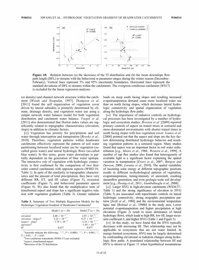
[35] HVG show less significant relationships with the be-havioral parameter ranges of the other seasons. This sug-gests that HVG is more related to the pattern of low flows,and effectively represents the level of water subsidy alonghydrologic flow paths during the growing season. Instead,the behavioral m ranges of deciduous headwater catch-ments during the winter season are significantly related tothe skewness of TI distribution and the mean DFL tostreams (Figure 10). Interestingly, the coniferous evergreencatchment (WS17) occupies distinct parameter spaces inFigure 10, where vegetation water use is still active evenduring the winter. The seasonal fluctuations of behavioral mparameter also reflect a structural deficiency of TOPMODELfrom the steady state assumption related to overestimation ofupslope contributing area especially during dry periods (theso-called dynamic a problem) [Beven and Freer, 2001]. Inaddition, high-elevation catchments also show very distinctRR, ET and HI values during the winter season (Figures 5c,5f, and 5i). These surely indicate that the flow levels

during the winter season are more related to catchmenttopology and topoclimatic factors rather than vegetationwater use.

3.5. Topographic Controls on HVG

[36] Two multiple regression models for HVG with topo-graphic variables are summarized in Table 3. The modelshows a higher R2 value without two coniferous catchments(WS01/17), which have very different phenological patternsand resulting seasonal patterns of evapotranspiration. Eleva-tion shows significant positive relationships with vegetationgradients in both models. This suggests that there is more lat-eral hydrologic connectivity at higher elevation, reflectingthe combined effect of orographic precipitation and environ-mental temperature lapse rate along the elevation gradient(Figure 2).

[37] The significance of the interaction term betweentransformed aspect and slope can be interpreted as strongradiative controls on hydrologic connectivity as this multi-plicative term is a typical radiation proxy parameter insteep terrain [Pierce et al., 2005]. More vegetation wateruse on south facing slopes results in less hydrologic con-nectivity during the growing season and smaller HVGwithin the catchment. This result is also consistent with thecomparison between two low-elevation control watershedsat different slopes (WS02/18).

[38] The skewness of TI distribution shows a significantnegative relationship with vegetation gradients for decidu-ous catchments (Table 3). Considering that the skewnesshas a significant negative relationship with the mean DFLto streams (Figure 4), it indicates that upslope subsidy maynot be used efficiently by downslope vegetation in hill-slopes with short DFL. Note that WS14, which has the

Figure 7. The relationships of hydrologic vegetation gradients (HVG) with (top) the intercept log(a)and (bottom) the slope b values from the regression slope analysis with different threshold values:(a) 0.01, (b) 0.1, (c) 0.2, and (d) 0.3 mm d�2.


10 of 16

Figure 8. Observed daily streamflow (black) and 5%/95% uncertainty boundaries (gray) from behav-ioral parameter ranges (Table 2) and their exceedance probabilities (%) for eight gauged headwatercatchments during 3 water year simulations (1991–1993; Table 2).


11 of 16

highest skewness and the lowest DFL values among gaugedcatchments (Figure 4), occupies a unique position duringthe summer season (Figure 9b). This can be interpreted as adominant geomorphic control on long-term hydrologic con-nectivity especially during the dormant season. The catch-ment area variable does not show any significance tovegetation gradients. This is consistent with previous stud-ies, which reported no significant effect of area on hydro-logic connectivity [McGlynn et al., 2004].

4. Discussion[39] In this study, HVG in headwater catchments are esti-

mated from fine resolution satellite imagery, and are relatedto hydrologic metrics, recession coefficients, and behavioralparameter ranges for a quasi-distributed ecohydrologicalmodel. Vegetation gradients are significantly correlated to an-nual hydrologic metrics (RR, ET, and HI). In addition, vege-tation gradients are also related to early recession behaviorrepresented by recession coefficients and behavioral parame-ter ranges of TOPMODEL. Increased vegetation densityalong hydrologic flow paths suggests substantial water sub-sidy from upslope to downslope especially through shallowsubsurface flow that is the main source of streamflow in thisregion [Hewlett and Hibbert, 1967]. On the contrary, static ordecreased vegetation density downslope indicates more local-ized water use by vegetation and less lateral hydrologic con-nectivity especially during the growing season. Specifically,negative HVG indicates that downslope vegetation may ex-perience more water stress because of associated temperatureincreases and orographic precipitation decreases at low eleva-tions. The decrease of NDVI downslope may also be relatedto low-NDVI species (e.g., rhododendron, eastern hemlock)

in cove region in the study area [Day et al., 1988; Bolstadet al., 1998a].

[40] The exponent b effectively represents the dominantflow regimes of upslope subsidy. The upslope subsidy incatchments with large HVG is dominated by shallow sub-surface flow, represented by large exponent b (around 1.5).The catchments with small HVG are probably more domi-nated by deeper groundwater flows as they behave like asimple linear storage system featured by small b (around1.0). Therefore, streams are disconnected from upslope,and hydrologic responses are spatially limited to the near-stream (riparian) dynamics in these catchments. There arefewer chances for upslope subsidy to be taken by vegeta-tion downslope, as the rooting depths in this region arequite shallow (around 1 m) and rather spatially uniform[Hales et al., 2009]. The early recession behavior is alsoclosely related to HVG. Smaller HVG headwater catch-ments usually have steeper early recessions, featured bylarge intercept, log(a) denoting more efficient drainage,and small behavioral m parameter ranges. Note that therecession behavior is not only associated with dominantflow regimes, but also with drainage efficiency of head-water catchments.

[41] We also found that the skewness of TI distributionhas a significant positive relationship with behavioral m pa-rameter ranges during the winter season (Figure 10a) and astatistically significant negative relationship with HVG fordeciduous catchments (Table 3). Considering that skewnessis a major factor determining the saturated fraction inTOPMODEL [Ducharne et al., 2000] as well as its rela-tionship with mean DFL to streams (Figure 4), it may beinterpreted as a significant geomorphic control on hydro-logic response. This is closely related to drainage efficiency

Figure 9. Relation between HVG and the behavioral ranges of two key TOPMODEL parameters(m and ln(T0)) during the full year (left column) and the summer season (JJA; right column).


12 of 16

(or density) and channel network structure within the catch-ment [Woods and Sivapalan, 1997]. Thompson et al.[2011] found the self organization of vegetation coverdriven by lateral subsidies is primarily determined by cli-mate, drainage density, and vegetation water use using asimple network water balance model for both vegetationdistribution and catchment water balance. Voepel et al.[2011] also demonstrated that Horton index values are sig-nificantly related to topographic characteristics (elevation,slope) in addition to climatic factors.

[42] Vegetation has priority for precipitation and soilwater through interception and transpiration [Brooks et al.,2010]. Therefore, vegetation patterns within headwatercatchments effectively represent the pattern of soil waterpartitioning between localized water use by vegetation (so-called green water) and lateral hydrologic flows (so-calledblue water). In this sense, green water downslope is par-tially dependent on the generation of blue water upslope.The interactive role of vegetation with hydrologic connec-tivity is first confirmed by the comparison of two first-order control catchments with opposite aspects (WS02/18;Table 1). In spite of the similarity in topographic character-istics and the amount of total precipitation, they have verydifferent RR, ET, and HI values (Figure 5), recessioncoefficients (Figure 7), and behavioral parameter spaces(Figure 9). We also found that the multiplicative term oftransformed aspect and slope has a significant negative rela-tion with vegetation gradients (Table 3). Greater radiation

loads on steep south facing slopes and resulting increasedevapotranspiration demand cause more localized water usethan on north facing slopes, which decreases lateral hydro-logic connectivity and spatial organization of vegetationalong the hydrologic flow paths.

[43] The importance of radiative controls on hydrologi-cal processes has been investigated by a number of hydro-logic and ecosystem studies. Broxton et al. [2009] reportedprimary controls of aspect on transit times in semiarid andsnow-dominated environments with shorter transit times insouth facing slopes with less vegetation cover. Ivanov et al.[2008] pointed out that the aspect and slope are the key fac-tors determining distributed hydrologic behavior and result-ing vegetation patterns in a semiarid region. Many studiesfound that aspect was an important factor in soil water redis-tribution [e.g., Moore et al., 1988; Western et al., 1999]. Anumber of sap flux studies also found that heterogeneity ofavailable light is a significant factor explaining the spatialvariation in transpiration [Ewers et al., 2007; Burgess andDawson, 2008; Loranty et al., 2010]. The spatial variabilityof incoming solar energy at different topographic positionsresults in different ecohydrological patterns of vegetation,evapotranspiration, timing/intensity of snowmelt, resultingstreamflow generation, and even geologic-scale soil develop-ment [e.g., Hwang et al., 2011; Istanbulluoglu et al., 2008].

[44] Larger HVG in high-elevation catchments (WS36/37;Table 1) and the strong significance of elevation to HVG(Table 3) are associated with topoclimatic controls on lateralhydrologic connectivity; strong orographic precipitation pat-terns [Swift et al., 1988] and the environmental temperaturelapse rate [Bolstad et al., 1998b] in the study area. Lowerpotential evapotranspiration and higher precipitation at highelevations (Figure 2) result in more dominance of lateralhydrologic flows, which leads to high RR, low HI, larger reces-sion coefficient b, and higher HVG (Table 1 and Figure 5).

[45] In this study, we have found that the HVG typicallydecreases with increasing HI. This relationship may not beapplicable in ecosystems that are not water limited. Inenergy-limited ecosystems, HVG may be largely determinedby confounding elevational or radiation changes along hydro-logic flow paths. A postulated relationship between HI andHVG is shown in Figure 11 when hypothetical mountainous

Figure 10. Relation between (a) the skewness of the TI distribution and (b) the mean downslope flowpath length (DFL) to streams with the behavioral m parameter ranges during the winter season (December–February). Vertical lines represent 5% and 95% uncertainty boundaries. Horizontal lines represent thestandard deviations of DFL to streams within the catchments. The evergreen coniferous catchment (WS17)is excluded for the linear regression analyses.

Table 3. Summary of Two Multiple Regression Models for theHydrologic Vegetation Gradient of Headwater Catchmentsa

Model 1 (n ¼ 20) Model 2b (n ¼ 18)

elevation 4.48 � 10�5 �� 2.87 � 10�5 ��

elevation : taspectc 5.22 � 10�5 � 9.27 � 10�5 ��

taspect : slopec �1.79 � 10�3 � �3.33 � 10�3 ��

skewnessd �1.85 � 10�2 ��

R2 0.637 0.877

aAsterisks indicate the following: ��, P < 0.0001; ��, P < 0.001; ��,P < 0.01; �, P < 0.05.

bTwo coniferous watersheds (WS01/17) are excluded.ctaspect, transformed aspect.dSkewness of the TI distribution.


13 of 16

headwater catchments would be located in different climateregions. In a snow-dominated climate region, the catchmentmay have the lowest HI as well as low vegetation gradients.In seasonally snow-dominated ecosystems, vegetationappears downslope first where temperatures are usuallyhigher. Tague [2009] also reported that the upslope subsidythrough seasonal snowmelts possibly decreased plant waterstress downslope in a mountainous watershed in the SierraNevada. In this case, the vegetation gradients increase withthe increase of HI, opposite to what is suggested in this study(Figure 5). In more water-limited regions, the vegetation gra-dients would decrease when HI increases.

[46] The high-elevation region in Coweeta may be moreenergy limited than water limited because of low tempera-ture and high precipitation. The region around the 1100–1300 m elevation band is usually regarded as the transitionzone from southern Appalachian to northern hardwood for-ests [Day et al., 1988]. Additionally, phenological featuresat high elevation are determined solely by temperature com-pared to low elevation [Hwang et al., 2011]. In this sense,the larger HVG in high-elevation south facing catchments(WS36/37) may be mostly driven by the accompanyingtemperature gradient downslope as well as the geomorphicgradient of steep, landslide dominated areas with limitedsoil cover compared to deeper, organic soils downslope[Band et al., 2012]. In addition, this may explain why wehave a relatively low vegetation gradient in the high-eleva-tion north facing catchment (WS27), with consistent energylimitations from ridge to valley. WS27 also lacks escarp-ments which drive the geomorphic gradients in soil depthand organic matter in WS36/37. It implies that HVG wouldbe highest in the ecotone region (Figure 11), where limitingfactors for vegetation growth vary along hydrologic flowpaths.

[47] This study implicitly assumes that water (or accom-panying nutrient) is a limiting resource for vegetation, andtherefore vegetation patterns are mainly determined by thelateral redistribution of soil water driven by dominant flowregimes. However, even when vegetation patterns are

determined by covarying factors along hydrologic flowpaths (e.g., temperature, radiation, and soils), emergentvegetation itself can be used to estimate the level of long-term partitioning between localized water use and lateralwater flow along hydrologic flow paths. In other words, theeffect of covarying factors is already manifested in emer-gent vegetation patterns. Note that HVG suggested in thisstudy is not intended for isolating the effect of soil moistureon vegetation density.

[48] Traditionally, in subhumid or humid mountainouscatchments hydrologists have focused more on the topo-graphic control of hydrologic processes [e.g., McGuireet al., 2005; Tetzlaff et al., 2009]. However, our study sug-gests that topography may exert primary controls overhydrologic response during high flows, while vegetationwater use has a significant effect on hydrologic connectiv-ity during the growing season. Therefore, the hydrologicresponse of watershed systems should be understood bycompetition between vegetation water use and drainage ef-ficiency [Thompson et al., 2011]. In this sense, this studysuggests that emergent vegetation patterns within head-water catchments may be used as a diagnostic tool tounderstand the interaction of local water balance (vegeta-tion water use or remnant soil recharge) along the hydro-logic flow paths with lateral redistribution.

5. Conclusions[49] In this study, we propose the hydrologic vegetation

gradient (HVG) as a simple indicator for lateral hydrologicconnectivity in a headwater catchment. HVG shows signifi-cant relationships with annual hydrologic metrics and thepatterns of flow regimes during the growing season. UsingHVG, we found dominant topoclimatic and geomorphologiccontrols on lateral hydrologic flows in the study area. With-out significant disturbance, the spatial organization of vege-tation within catchments effectively represents the degree ofdependency of ecosystems along hydrologic flow paths.This study also presents the potential to estimate earlyrecession behavior, and key model parameters of ungaugedheadwater catchments from remotely sensed HVG.

[50] Acknowledgments. We thank the Editor, Michael L. Roderick,and two anonymous reviewers for constructive comments. The researchrepresented in this paper was supported by the National Science Founda-tion award to the Coweeta Long Term Ecologic Research project (DEB0823293). The USDA Forest Service provides long-term streamflow andclimate data, as well as access and facilities at the Coweeta HydrologicLaboratory.

ReferencesAli, G. A., and A. G. Roy (2010), Shopping for hydrologically representa-

tive connectivity metrics in a humid temperate forested catchment, WaterResour. Res., 46, W12544, doi:10.1029/2010WR009442.

Asrar, G., M. Fuchs, E. T. Kanemasu, and J. L. Hatfield (1984), Estimatingabsorbed photosynthetic radiation and leaf-area index from spectral re-flectance in wheat, Agron. J., 76, 300–306.

Asrar, G., R. B. Myneni, and B. J. Choudhury (1992), Spatial heterogeneityin vegetation canopies and remote-sensing of absorbed photosyntheti-cally active radiation—A modeling study, Remote Sens. Environ., 41,85–103.

Band, L. E., P. Patterson, R. Nemani, and S. W. Running (1993), Forestecosystem processes at the watershed scale: Incorporating hillslope hy-drology, Agric. For. Meteorol., 63, 93–126.

Band, L. E., T. Hwang, T. C. Hales, J. Vose, and C. Ford (2012), Ecosystemprocesses at the watershed scale: Mapping and modeling ecohydrological

Figure 11. A postulated relationship between Hortonindex and HVG. ET, evapotranspiration; PET, potentialevapotranspiration.


14 of 16

controls of landslides, Geomorphology, 137, 159–167, doi:10.1016/j.geomorph.2011.06.025.

Beers, T. W., P. E. Dress, and L. C. Wensel (1966), Aspect transformationin site productivity research, J. For., 64, 691–692.

Beven, K., and A. Binley (1992), The future of distributed models: Modelcalibration and uncertainty prediction, Hydrol. Processes, 6, 279–298.

Beven, K., and J. Freer (2001), A dynamic TOPMODEL, Hydrol. Proc-esses, 15, 1993–2011.

Beven, K., and M. Kirkby (1979), A physically-based variable contributingarea model of basin hydrology, Hydrol. Sci. Bull., 24, 43–69.

Bolstad, P. V., W. Swank, and J. Vose (1998a), Predicting southern Appala-chian overstory vegetation with digital terrain data, Landscape Ecol., 13,271–283, doi:10.1023/A:1008060508762.

Bolstad, P. V., L. Swift, F. Collins, and J. Regniere (1998b), Measured andpredicted air temperatures at basin to regional scales in the southern Ap-palachian mountains, Agric. For. Meteorol., 91, 161–176.

Bolstad, P. V., J. M. Vose, and S. G. McNulty (2001), Forest productivity,leaf area, and terrain in southern Appalachian deciduous forests, For.Sci., 47, 419–427.

Bond, B. J., J. A. Jones, G. Moore, N. Phillips, D. Post, and J. J. McDonnell(2002), The zone of vegetation influence on baseflow revealed by dietpatterns of streamflow and vegetation water use in a headwater basin,Hydrol. Processes, 16, 1671–1677, doi:10.1002/hyp.5022.

Bracken, L. J., and J. Croke (2007), The concept of hydrological con-nectivity and its contribution to understanding runoff-dominated geo-morphic systems, Hydrol. Processes, 21, 1749–1763, doi:10.1002/hyp.6313.

Brooks, J. R., H. R. Barnard, R. Coulombe, and J. J. McDonnell (2010),Ecohydrologic separation of water between trees and streams in a Medi-terranean climate, Nat. Geosci., 3, 100–104, doi:10.1038/NGEO722.

Brooks, P. D., P. A. Troch, M. Durcik, E. Gallo, and M. Schlegel (2011),Quantifying regional scale ecosystem response to changes in precipita-tion: Not all rain is created equal, Water Resour. Res., 47, W00J08,doi:10.1029/2010WR009762.

Broxton, P. D., P. A. Troch, and S. W. Lyon (2009), On the role of aspect toquantify water transit times in small mountainous catchments, WaterResour. Res., 45, W08427, doi:10.1029/2008WR007438.

Brutsaert, W., and J. P. Lopez (1998), Basin-scale geohydrologic droughtflow features of riparian aquifers in the Southern Great Plains, WaterResour. Res., 34, 233–240, doi:10.1029/97WR03068.

Brutsaert, W., and J. L. Nieber (1977), Regionalized drought flow hydro-graphs from a mature glaciated plateau, Water Resour. Res., 13, 637–644, doi:10.1029/WR013i003p00637.

Burgess, S. S. O., and T. E. Dawson (2008), Using branch and basal trunksap flow measurements to estimate whole-plant water capacitance: Acaution, Plant Soil, 305, 5–13, doi:10.1007/s11104-007-9378-2.

Chen, J. M., and T. A. Black (1992), Defining leaf-area index for non-flatleaves, Plant Cell Environ., 15, 421–429.

Clark, J. S., D. M. Bell, M. H. Hersh, and L. Nichols (2011), Climatechange vulnerability of forest biodiversity: Climate and competitiontracking of demographic rates, Global Change Biol., 17, 1834–1849,doi:10.1111/j.1365-2486.2010.02380.x.

Day, F. P., and C. D. Monk (1974), Vegetation patterns on a southern Appa-lachian watershed, Ecology, 55, 1064–1074.

Day, F. P., D. L. Philips, and C. D. Monk (1988), Forest communities andpatterns, in Forest Hydrology and Ecology at Coweeta, edited by W. T.Swank and D. A. Crossley Jr., pp. 141–149, Springer, New York.

Detty, J. M., and K. J. McGuire (2010), Topographic controls on shallowgroundwater dynamics: Implications of hydrologic connectivity betweenhillslopes and riparian zones in a till mantled catchment, Hydrol. Proc-esses, 24, 2222–2236, doi:10.1002/hyp.7656.

Ducharne, A., R. D. Koster, M. J. Suarez, M. Stieglitz, and P. Kumar(2000), A catchment-based approach to modeling land surface processesin a general circulation model: 2. Parameter estimation and model dem-onstration, J. Geophys. Res., 105, 24,823–24,838.

Eberbach, P. L., and G. E. Burrows (2006), The transpiration response byfour topographically distributed Eucalyptus species, to rainfall occurringduring drought in south eastern Australia, Physiol. Plant., 127, 483–493,doi:10.1111/j.1399-3054.2006.00762.x.

Eckhardt, K. (2005), How to construct recursive digital filters for baseflowseparation, Hydrol. Processes, 19, 507–515, doi:10.1002/hyp.5675.

Ewers, B. E., R. Oren, H. S. Kim, G. Bohrer, and C. T. Lai (2007), Effectsof hydraulic architecture and spatial variation in light on mean stomatalconductance of tree branches and crowns, Plant Cell Environ., 30, 483–496, doi:10.1111/j.1365-3040.2007.01636.x.

Ford, C. R., R. M. Hubbard, B. D. Kloeppel, and J. M. Vose (2007), A com-parison of sap flux-based evapotranspiration estimates with catchment-scale water balance, Agric. For. Meteorol., 145, 176–185, doi:10.1016/j.agrformet.2007.04.010.

Freer, J., K. Beven, and B. Ambroise (1996), Bayesian estimation of uncer-tainty in runoff prediction and the value of data: An application of theGLUE approach, Water Resour. Res., 32, 2161–2173.

Freer, J., K. Beven, and N. Peters (2004), Multivariate seasonal periodmodel rejection within the generalised likelihood uncertainty estimationprocedure, in Calibration of Watershed Models, Water Sci. Appl., vol. 6,edited by Q. Duan et al., pp. 69–87, AGU, Washington, D. C.

Grayson, R. B., A. W. Western, F. H. S. Chiew, and G. Bloschl (1997),Preferred states in spatial soil moisture patterns: Local and nonlocalcontrols, Water Resour. Res., 33, 2897–2908.

Hales, T. C., C. R. Ford, T. Hwang, J. M. Vose, and L. E. Band (2009),Topographic and ecologic controls on root reinforcement, J. Geophys.Res., 114, F03013, doi:10.1029/2008JF001168.

Harman, C. J., M. Sivapalan, and P. Kumar (2009), Power law catchment-scale recessions arising from heterogeneous linear small-scale dynamics,Water Resour. Res., 45, W09404, doi:10.1029/2008WR007392.

Hewlett, J. D., and A. R. Hibbert (1967), Factors affecting the response ofsmall watersheds to precipitation in humid areas, in Forest Hydrology,edited by N. E. Sopper and H. W. Lull, pp. 275–290, Pergamon, NewYork.

Hirsch, R. M., and E. J. Gilroy (1984), Methods of fitting a straight line todata: Examples in water resources, Water Resour Bull., 20, 705–711.

Hopp, L., and J. J. McDonnell (2009), Connectivity at the hillslope scale:Identifying interactions between storm size, bedrock permeability, slopeangle and soil depth, J. Hydrol., 376, 378–391, doi:10.1016/j.jhydrol.2009.07.047.

Horton, R. E. (1933), The role of infiltration in the hydrologic cycle, EosTrans. AGU, 14, 446–460.

Hwang, T., L. E. Band, and T. C. Hales (2009), Ecosystem processes at thewatershed scale: Extending optimality theory from plot to catchment,Water Resour. Res., 45, W11425, doi:10.1029/2009WR007775.

Hwang, T., C. Song, J. M. Vose, and L. E. Band (2011), Topography-mediated controls on local vegetation phenology estimated from MODISvegetation index, Landscape Ecol., 26, 541–556, doi:10.1007/s10980-011-9580-8.

Istanbulluoglu, E., O. Yetemen, E. R. Vivoni, H. A. Gutierrez-Jurado, andR. L. Bras (2008), Eco-geomorphic implications of hillslope aspect:Inferences from analysis of landscape morphology in central New Mex-ico, Geophys. Res. Lett., 35, L14403, doi:10.1029/2008GL034477.

Ivanov, V. Y., R. L. Bras, and E. R. Vivoni (2008), Vegetation-hydrologydynamics in complex terrain of semiarid areas: 2. Energy-water controlsof vegetation spatiotemporal dynamics and topographic niches of favor-ability, Water Resour. Res., 44, W03430, doi:10.1029/2006WR005595.

James, A. L., and N. T. Roulet (2007), Investigating hydrologic connectiv-ity and its association with threshold change in runoff response in a tem-perate forested watershed, Hydrol. Processes, 21, 3391–3408, doi:10.1002/hyp.6554.

Jencso, K. G., B. L. McGlynn, M. N. Gooseff, S. M. Wondzell, K. E.Bencala, and L. A. Marshall (2009), Hydrologic connectivity betweenlandscapes and streams: Transferring reach-and plot-scale understandingto the catchment scale, Water Resour. Res., 45, W04428, doi:10.1029/2008WR007225.

Kokkonen, T. S., A. J. Jakeman, P. C. Young, and H. J. Koivusalo (2003),Predicting daily flows in ungauged catchments: Model regionalizationfrom catchment descriptors at the Coweeta Hydrologic Laboratory,North Carolina, Hydrol. Processes, 17, 2219–2238.

Law, B. E., et al. (2002), Environmental controls over carbon dioxide andwater vapor exchange of terrestrial vegetation, Agric. For. Meteorol.,113, 97–120.

Lim, K. J., B. A. Engel, Z. X. Tang, J. Choi, K. S. Kim, S. Muthukrishnan,and D. Tripathy (2005), Automated Web GIS based hydrograph analysistool, WHAT, J. Am. Water Resour. Assoc., 41, 1407–1416.

Lindsay, J. B. (2005), The Terrain Analysis System: A tool for hydro-geo-morphic applications, Hydrol. Processes, 19, 1123–1130.

Loranty, M. M., D. S. Mackay, B. E. Ewers, E. Traver, and E. L. Kruger(2010), Contribution of competition for light to within-species variabilityin stomatal conductance, Water Resour. Res., 46, W05516, doi:10.1029/2009WR008125.

Ludwig, J. A., B. P. Wilcox, D. D. Breshears, D. J. Tongway, and A. C.Imeson (2005), Vegetation patches and runoff-erosion as interacting eco-hydrological processes in semiarid landscapes, Ecology, 86, 288–297.


15 of 16

Mackay, D. S., and L. E. Band (1997), Forest ecosystem processes at thewatershed scale: Dynamic coupling of distributed hydrology and canopygrowth, Hydrol. Processes, 11, 1197–1217.

Mackay, D. S., B. E. Ewers, M. M. Loranty, and E. L. Kruger (2010), Onthe representativeness of plot size and location for scaling transpirationfrom trees to a stand, J. Geophys. Res., 115, G02016, doi:10.1029/2009JG001092.

McGlynn, B. L., J. J. McDonnell, J. Seibert, and C. Kendall (2004), Scaleeffects on headwater catchment runoff timing, flow sources, and ground-water-streamflow relations, Water Resour. Res., 40, W07504, doi:10.1029/2003WR002494.

McGuire, K. J., and J. J. McDonnell (2010), Hydrological connectivity ofhillslopes and streams: Characteristic time scales and nonlinearities,Water Resour. Res., 46, W10543, doi:10.1029/2010WR009341.

McGuire, K. J., J. J. McDonnell, M. Weiler, C. Kendall, B. L. McGlynn,J. M. Welker, and J. Seibert (2005), The role of topography on catchment-scale water residence time, Water Resour. Res., 41, W05002, doi:10.1029/2004WR003657.

Moore, I. D., G. J. Burch, and D. H. Mackenzie (1988), Topographic effectson the distribution of surface soil-water and the location of ephemeralgullies, Trans. ASAE, 31, 1098–1107.

Myneni, R. B., and D. L. Williams (1994), On the relationship betweenFAPAR and NDVI, Remote Sens. Environ., 49, 200–211.

Myneni, R. B., et al. (2002), Global products of vegetation leaf area andfraction absorbed PAR from year one of MODIS data, Remote Sens. En-viron., 83, 214–231.

Nash, J. E., and J. V. Sutcliffe (1970), River flow forecasting throughconceptual models part I—A discussion of principles, J. Hydrol., 10,282–290.

Pierce, K. B., T. Lookingbill, and D. Urban (2005), A simple method forestimating potential relative radiation (PRR) for landscape-scale vegeta-tion analysis, Landscape Ecol., 20, 137–147, doi:10.1007/s10980-004-1296-6.

Post, D. A., J. A. Jones, and G. E. Grant (1998), An improved methodologyfor predicting the daily hydrologic response of ungauged catchments, En-viron. Modell. Software, 13, 395–403.

Price, K., C. R. Jackson, and A. J. Parker (2010), Variation of surficial soilhydraulic properties across land uses in the southern Blue Ridge Moun-tains, North Carolina, USA, J. Hydrol., 383, 256–268, doi:10.1016/j.jhydrol.2009.12.041.

Pringle, C. (2003), What is hydrologic connectivity and why is it ecologicallyimportant?, Hydrol. Processes, 17, 2685–2689, doi:10.1002/hyp.5145.

Rupp, D. E., and J. S. Selker (2006a), Information, artifacts, and noise indQ/dt � Q recession analysis, Adv. Water Resour., 29, 154–160,doi:10.1016/j.advwatres.2005.03.019.

Rupp, D. E., and J. S. Selker (2006b), On the use of the Boussinesq equationfor interpreting recession hydrographs from sloping aquifers, WaterResour. Res., 42, W12421, doi:10.1029/2006WR005080.

Sellers, P. J. (1985), Canopy reflectance, photosynthesis and transpiration,Int. J. Remote Sens., 6, 1335–1372.

Swift, L. W., G. B. Cunningham, and J. E. Douglass (1988), Climatologyand hydrology, in Forest Hydrology and Ecology at Coweeta, edited byW. T. Swank and D. A. Crossley Jr., pp. 35–55, Springer, New York.

Szilagyi, J., Z. Gribovszki, and P. Kalicz (2007), Estimation of catchment-scale evapotranspiration from baseflow recession data: Numerical modeland practical application results, J. Hydrol., 336, 206–217, doi:10.1016/j.jhydrol.2007.01.004.

Tague, C. L. (2009), Assessing climate change impacts on alpine stream-flow and vegetation water use: Mining the linkages with subsurface hydro-logic processes, Hydrol. Processes, 23, 1815–1819, doi:10.1002/hyp.7288.

Tague, C. L., and L. E. Band (2004), RHESSys: Regional Hydro-EcologicSimulation System—An object-oriented approach to spatially distributedmodeling of carbon, water, and nutrient cycling, Earth Interact., 8(19),1–42, doi:10.1175/1087-3562(2004)8<1:RRHSSO>2.0.CO;2.

Tague, C., and G. E. Grant (2004), A geological framework for interpretingthe low-flow regimes of Cascade streams, Willamette River Basin, Ore-gon, Water Resour. Res., 40, W04303, doi:10.1029/2003WR002629.

Tarboton, D. G. (1997), A new method for the determination of flow direc-tions and upslope areas in grid digital elevation models, Water Resour.Res., 33, 309–319.

Tetzlaff, D., J. Seibert, K. J. McGuire, H. Laudon, D. A. Burn, S. M. Dunn,and C. Soulsby (2009), How does landscape structure influence catch-ment transit time across different geomorphic provinces?, Hydrol. Proc-esses, 23, 945–953, doi:10.1002/hyp.7240.

Tetzlaff, D., C. Soulsby, and C. Birkel (2010), Hydrological connectivity andmicrobiological fluxes in montane catchments: The role of seasonality andclimatic variability, Hydrol. Processes, 24, 1231–1235, doi:10.1002/hyp.7680.

Thompson, S. E., C. J. Harman, P. A. Troch, P. D. Brooks, and M. Sivapalan(2011), Spatial scale dependence of ecohydrologically mediated waterbalance partitioning: A synthesis framework for catchment ecohydrology,Water Resour. Res., 47, W00J03, doi:10.1029/2010WR009998.

Troch, P. A., G. F. Martinez, V. R. N. Pauwels, M. Durcik, M. Sivapalan,C. Harman, P. D. Brooks, H. Gupta, and T. Huxman (2009), Climate andvegetation water use efficiency at catchment scales, Hydrol. Processes,23, 2409–2414, doi:10.1002/hyp.7358.

Voepel, H., B. Ruddell, R. Schumer, P. A. Troch, P. D. Brooks, A. Neal, M.Durcik, and M. Sivapalan (2011), Quantifying the role of climate and land-scape characteristics on hydrologic partitioning and vegetation response,Water Resour. Res., 47, W00J09, doi:10.1029/2010WR009944.

Vose, J. M., and W. T. Swank (1990), Assessing seasonal leaf-area dynamicsand vertical leaf-area distribution in eastern white pine (Pinus strobus L.)with a portable light meter, Tree Physiol., 7, 125–134.

Vose, J. M., P. M. Dougherty, J. N. Long, F. W. Smith, H. L. Gholz, andP. J. Curran (1994), Factors influencing the amount and distribution ofleaf area of pine stands, Ecol. Bull., 43, 102–114.

Wagener, T., and H. S. Wheater (2006), Parameter estimation and regional-ization for continuous rainfall-runoff models including uncertainty, J.Hydrol., 320, 132–154, doi:10.1016/j.jhydrol.2005.07.015.

Webb, W., S. Szarek, W. Lauenroth, R. Kinerson, and M. Smith (1978),Primary productivity and water-use in native forest, grassland, and desertecosystems, Ecology, 59, 1239–1247, doi:10.2307/1938237.

Western, A. W., R. B. Grayson, G. Bloschl, G. R. Willgoose, and T. A.McMahon (1999), Observed spatial organization of soil moisture and itsrelation to terrain indices, Water Resour. Res., 35, 797–810.

Western, A. W., G. Bloschl, and R. B. Grayson (2001), Toward capturinghydrologically significant connectivity in spatial patterns, Water Resour.Res., 37, 83–97.

Whittaker, R. H. (1956), Vegetation of the Great Smoky Mountains, Ecol.Monogr., 26, 1–69.

Wigmosta, M. S., L. W. Vail, and D. P. Lettenmaier (1994), A distributedhydrology-vegetation model for complex terrain, Water Resour. Res., 30,1665–1679.

Woods, R. A., and M. Sivapalan (1997), A connection between topographi-cally driven runoff generation and channel network structure, WaterResour. Res., 33, 2939–2950.

Yeakley, J. A., W. T. Swank, L. W. Swift, G. M. Hornberger, and H. H.Shugart (1998), Soil moisture gradients and controls on a southern Appa-lachian hillslope from drought through recharge, Hydrol. Earth Syst.Sci., 2, 41–49.


16 of 16

ecosystem processes at the watershed scale: hydrologic vegetation

Documents