1

EDC1

1.0 EDC Problem Formulation

Each plant i has a cost-rate curve that gives

the cost Ci in $/hour as a function of its

generation level PGi (the 3 phase power). So

we denote the cost-rate functions as Ci(PGi).

These functions are often assumed to be

quadratic (and therefore convex). For

example, two such functions are given as 2

1111 01.045900)( GGG PPPC (1) 2

2221 003.0432500)( GGG PPPC (2)

If we have m generating units, then the total

system cost will be given by

)(1

Gi

m

i

iT PCC

(3)

Equation (3), represents our objective

function, and we desire to minimize it. The

generation values PGi are the decision

variables.

2

There are two basic kinds of constraints for

our problem.

1.Power balance

2.Generation limits

1.1 Power balance constraint

In regards to power balance, it must be the

case that the total generation equals the total

demand PD plus the total losses PL.

LD

m

i

Gi PPP 1

(4a)

The demand PD is assumed to be a fixed

value. However, the losses PL depend on the

solution (given by the PGi) which we do not

know until we solve the problem. This

dependency is due to the fact that the losses

depend on the flows in the circuits, and the

flows in the circuits depend on the

generation dispatch. Therefore we represent

this dependency according to eq. (4b).

),,,( 21

1

GmGGLD

m

i

Gi PPPPPP

(4b)

3

Note that only m-1 of the PGi are

independent variables. Given demand and

losses, one of the generation values is

determined once the other m-1 of them are

set. We will assume this generator is unit 1.

Therefore we need to remove PG1 from the

arguments of PL so that eq. (4b) becomes

),,( 2

1

GmGLD

m

i

Gi PPPPP

(4c)

We rearrange eq. (4c) so that all terms

dependent of the decision variables are on

the left-hand-side, according to:

DGmGL

m

i

Gi PPPPP

),,( 2

1

(4d)

1.2 Generation limits

There are physical constraints on the

generation levels. The generators cannot

exceed their maximum capabilities,

represented by max

GiP . And clearly, they

cannot operate below 0 (otherwise they are

4

operating as a motor, attempting to drive the

turbine – not a good operational state!).

Most units actually cannot operate at 0; as a

result, we will denote the minimum as min

GiP .

Therefore, the generation limits are

represented by maxmin

GiGiGi PPP (5)

1.3 Problem statement

This leads us to the statement of the

problem, i.e., the articulation of the

mathematical program, which is, from eqs.

(3), (4d), and (5), as follows.

Min )(

1

Gi

m

i

iT PCC

Subject to

DGmGL

m

i

Gi PPPPP

),,( 2

1

miPPP GiGiGi ,...,1maxmin ,...,miPGi 10

5

2.0 Application of KKT conditions In formulating the KKT conditions, we recall

that the complementary condition is handled

procedurally as below.

Solve the problem without any inequality

constraint

Check solution against inequality constraints.

For those that are violated, bring them in as

equality constraints and re-solve the problem.

Repeat this step until you obtain a solution

for which no inequality constraints are

violated.

This is an iterative solution procedure, and

represents a procedural equivalent to the

complementary condition. Thus, for any given

iteration, we can assume there are no

inequality constraints.

Therefore we may state the required

conditions for the solution more simply as

nix

F

i

,10

(6)

JjF

j

,10

(7)

6

where it is assumed that any binding

inequality constraints are included in eq. (7)

as equality constraints.

Let’s apply these conditions to the problem

statement of Section 1.3 above, assuming

that no inequality constraints are binding so

that there is only one equality constraint to

consider (the power balance constraint).

First, we form the Lagrangian function:

DGmGL

m

i

GiGi

m

i

i PPPPPPCF ),,()( 2

11

(8)

Now applying the KKT conditions of (6)

and (7), we get:

miP

PPP

P

PC

P

F

Gi

GmGL

Gi

Gii

Gi

,...1,0),,(

1)( 2

(9)

0),,( 2

1

DGmGL

m

i

Gi PPPPPF

(10)

Observe that we have m equations of the

form given in (9). However, the one

7

corresponding to i=1 will not have a loss

term and therefore will be:

0)(

1

11

1

G

Gi

G P

PC

P

F (11)

Because 01

P

PL

, eq. (9) appropriately

captures eq. (11).

The term Gi

i

P

C

is the incremental cost of unit i

and is denoted by ICi.

Let’s consider eq. (9) more closely. In

particular, let’s solve it for λ.

miP

PC

P

PPP Gi

Gii

Gi

GmGL

,...1)(

),,(1

1

2

(12)

Define the fraction out front as Li, that is

Gi

GmGL

i

P

PPPL

),,(1

1

2 (13)

We call Li the penalty factor for the ith unit.

Note that L1=1.

8

Substituting eq. (13) into (12) results in

miP

PCL

Gi

Giii ,...1

)(

(14)

What eq. (14) says is that, at the optimum

dispatch, for each unit not at a binding

inequality constraint, the product of the

penalty factor and the incremental cost of

unit is the same and is equal to λ.

Example:

Consider the cost-rate functions: 2

1111 01.045900)( GGG PPPC (1) 2

2221 003.0432500)( GGG PPPC (2)

The load is specified as PD=600 MW.

Generator limits are given as

MWPMW G 20050 1

MWPMW G 60050 1

In this example, we assume that there are no

losses. This means that all penalty factors

are 1.0. Assuming there are no binding

inequality constraints, eq. (14) is

2

22

1

11 )()(

G

G

G

G

P

PC

P

PC

9

Writing out these equations, we have:

102.045 GP

2006.043 GP

We also have our equality constraint eq. (10)

60021 GG PP

We can solve these equations in matrix

representation, as a set of linear equations,

as given below.

600

43

45

011

1006.00

1002.0

2

1

G

G

P

P

Solution to this equation yields:

23.46

46.538

64.61

2

1

G

G

P

P

Checking the inequality limits, we see that

we have found the solution.

Let’s explore another solution method.

The previous one is fine, but it requires that

all equations be linear. This may not always

be the case, e.g., when we include losses, the

power balance equation can be nonlinear.

10

The method is known as Lambda-iteration

and is best understood via Fig. 1 which

shows incremental cost curves IC1, IC2,

given by

11 02.045 GPIC

22 006.043 GPIC

The incremental cost curves are just the

derivatives of the cost-rate curves. Observe

that the expressions derived for λ under the

KKT conditions specify a certain relation

among the incremental cost curves. An

implication here is that the incremental cost

curves express the derivatives (or the

incremental costs) under any condition, not

necessarily at the optimum.

11

0 100 200 300 400 500 60043

44

45

46

47

48

49

MW

$/M

Whr

IC1=45+0.02Pg1

IC2=43+0.006Pg2

Fig. 1

The lambda iteration method begins with a

guess in regards to a value of λ which

satisfies the KKT conditions (such that all

incremental costs are equal), and the total

demand equals the load.

The lambda iteration may be performed

graphically. Let’s guess that λ=46. To

determine what the corresponding

generation levels are at the optimum, draw a

12

horizontal line across our IC curves, as

shown by the dark horizontal line in Fig. 2.

0 100 200 300 400 500 60043

44

45

46

47

48

49

MW

$/M

Whr

IC1=45+0.02Pg1

IC2=43+0.006Pg2

Fig. 2

The corresponding generation values are the

dark vertical dashed lines, so we can see that

PG1=50 and PG2=500, for a total generation

of 550 MW. This is less than the desired

600 MW so let’s increase our guess. Let’s

try about 46.4, as shown in Fig. 3.

13

0 100 200 300 400 500 60043

44

45

46

47

48

49

MW

$/M

Whr

IC1=45+0.02Pg1

IC2=43+0.006Pg2

Fig. 3

The corresponding generation levels are

about PG1=65 MW and PG2=565 MW, for a

total of 630 MW, and so this is a little too

high. Let’s try λ=46.2 as shown in Fig. 4.

14

0 100 200 300 400 500 60043

44

45

46

47

48

49

MW

$/M

Whr

IC1=45+0.02Pg1

IC2=43+0.006Pg2

Fig. 4

The corresponding generation levels are

about PG1=55 MW and PG2=540 MW for a

total of 595 MW, so this is just a small bit

too low. It is probably not possible to do

better than this unless we use a more

granular axis in our plots.

This method can be stated analytically as

well. Notice what we are doing: we choose λ

and then obtain the generation levels from

the plots.

15

The plots are really analytical relations

between λ and the generation levels, and we

can easily manipulate them so that they give

the generation levels as a function of λ, as

shown below.

2250504502.0 11 GG PP

7.716667.16643006.0 22 GG PP

Now we can proceed analytically.

As before, guess 46 and calculate:

502250)46(501 GP

5007.7166)46(67.1662 GP

Total is 550 MW which is too low so let’s

try 46.4 (we could try anything we like, as

long as it is higher, since the generation is

too low in our first guess):

702250)4.46(501 GP

78.5667.7166)4.46(67.1662 GP

Total is 636.78, so now we need to try a

lower λ. But let’s use linear interpolation to

guide our next value of λ:

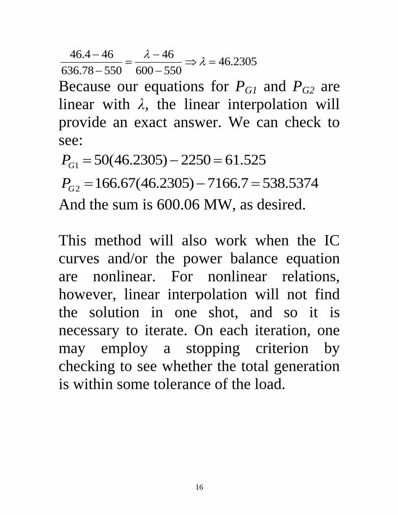
16

2305.46550600

46

55078.636

464.46

Because our equations for PG1 and PG2 are

linear with λ, the linear interpolation will

provide an exact answer. We can check to

see:

525.612250)2305.46(501 GP

5374.5387.7166)2305.46(67.1662 GP

And the sum is 600.06 MW, as desired.

This method will also work when the IC

curves and/or the power balance equation

are nonlinear. For nonlinear relations,

however, linear interpolation will not find

the solution in one shot, and so it is

necessary to iterate. On each iteration, one

may employ a stopping criterion by

checking to see whether the total generation

is within some tolerance of the load.

17

Example (extended):

Now let’s reconsider our example, but with

a load of 700 MW instead of 600 MW.

Using our graphical method again, and with

the knowledge gained from our previous

example, we know that λ will exceed 46.4.

But it cannot go too much higher without

causing Unit 2 to exceed its upper limit.

Let’s try it at the value of λ that causes unit

2 to be at its upper limit. This is shown in

Fig. 5.

0 100 200 300 400 500 60043

44

45

46

47

48

49

MW

$/M

Whr

IC1=45+0.02Pg1

IC2=43+0.006Pg2

Fig. 5

18

It appears that λ is about 46.6, and PG1≈85

MW, PG2≈600 MW, for a total of 685 MW.

So this is not enough, and we must therefore

raise λ. However, we cannot raise λ on unit 2

because it is already at its upper limit. So we

have to clamp PG2 at 600 MW. In other

words, we will no longer use PG2 in our λ-

iteration, although we will need to account

for its generation of 600 MW.

So we will now perform λ-iteration on only

the remaining units. In this case, the

“remaining units” is just unit 1. In addition,

our stopping criteria will now be that the

total generation of the remaining units be

equal to PD-Pg2=700-600=100.

The upshot of this is that we need to perform

λ-iteration on unit 1’s ability to supply 100

MW. The horizontal solid-dark line of Fig. 6

illustrates.

19

0 100 200 300 400 500 60043

44

45

46

47

48

49

MW

$/M

Whr

IC1=45+0.02Pg1

IC2=43+0.006Pg2

Fig. 5

Observe, however that there are now two

horizontal lines,

the solid one for unit 1 at 47;

the dashed one for unit 2 at about 46.6

So which one is λ?

λ is the SYSTEM incremental cost and

indicates the cost of optimally supplying another

MW from the system for the next hour. If the

system has to supply another MW for the next

hour, in this case (because there is only 1

regulating unit), it would have no choice but to

do it with unit 1.

Therefore λ=47.

20

Then what is 46.6? It is the incremental cost of

unit 2 (but not the system incremental cost).

The unit incremental cost is normally

understood as the cost for the unit to supply

another MW for one hour. It can equivalently

be understood as the savings if the unit was

off-loaded by 1 MW for one hour, and in this

case, that is a better interpretation since the

unit cannot supply more power.

Let’s look at this example in terms of a real-

time market. In this case, the generator offer

curves might appear as in Fig. 6.

0 100 200 300 400 500 60043

44

45

46

47

48

49

MW

$/M

Whr

IC1=45+0.02Pg1

IC2=43+0.006Pg2

Fig. 6

21

The stacked offers appear as in Table 1. Offer/bid

order

Offers to sell 1 MWhr

Seller Quantity

(MW)

Price

($/MWhr)

1 S2 100 43.9

2 S2 100 44.5

3 S2 100 45.1

4 S2 100 45.6

5 S2 100 46.3

6 S2 100 46.6

7 S1 25 46.6

8 S1 25 47.0

9 S1 25 47.5

10 S1 25 48.0

11 S1 25 48.5

12 S1 25 49.0

Observe that with this representation, the

700 MW solution would not change from

that which we obtained from the linear

incremental cost curves.

However, the 600 MW solution might differ,

depending on “market rules” which would

need to decide whether to award the last 25

MW to S1 or to S2. If it awarded it to S1,

then the solution would be Pg1=75MW,

Pg2=515 MW. This is about what we got in

the solution with linear incremental costs

(Pg1=61.5MW, Pg2=538.5MW), the

22

difference caused by the approximation

made by the step functions associated with

the market offers. This approximation can

be reduced by taking smaller “steps” in the

incremental cost curve.

It is necessary to represent the offers in this

stepwise approach in order to maintain

linearity in the objective function and

consequently enable solution by linear

programming. If one utilized the linear

incremental cost functions, then the

objective functions would have quadratics,

as we have seen in this example.