edge detection edge detection
TRANSCRIPT
1
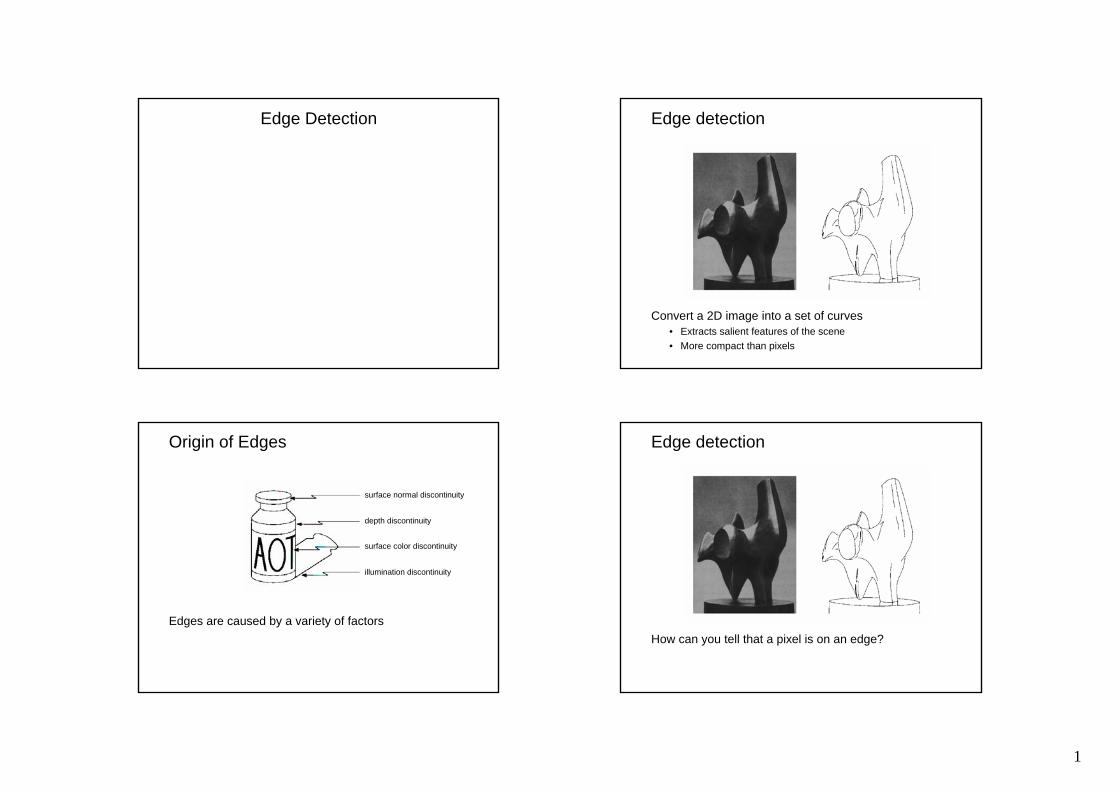
Edge Detection Edge detection
Convert a 2D image into a set of curves• Extracts salient features of the scene• More compact than pixels
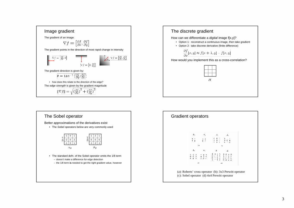
Origin of Edges
Edges are caused by a variety of factors
depth discontinuity
surface color discontinuity
illumination discontinuity
surface normal discontinuity
Edge detection
How can you tell that a pixel is on an edge?

2
Profiles of image intensity edges Edge detection1. Detection of short linear edge segments (edgels)
2. Aggregation of edgels into extended edges(maybe parametric description)
Edgel detection
• Difference operators
• Parametric-model matchers
Edge is Where Change OccursChange is measured by derivative in 1DBiggest change, derivative has maximum magnitudeOr 2nd derivative is zero.
3
Image gradientThe gradient of an image:
The gradient points in the direction of most rapid change in intensity
The gradient direction is given by:
• how does this relate to the direction of the edge?The edge strength is given by the gradient magnitude
The discrete gradientHow can we differentiate a digital image f[x,y]?
• Option 1: reconstruct a continuous image, then take gradient• Option 2: take discrete derivative (finite difference)
How would you implement this as a cross-correlation?
The Sobel operatorBetter approximations of the derivatives exist
• The Sobel operators below are very commonly used
10-120-2
10-1
-1-2-1000
121
• The standard defn. of the Sobel operator omits the 1/8 term– doesn’t make a difference for edge detection– the 1/8 term is needed to get the right gradient value, however
Gradient operators
(a): Roberts’ cross operator (b): 3x3 Prewitt operator(c): Sobel operator (d) 4x4 Prewitt operator
4
Effects of noiseConsider a single row or column of the image
• Plotting intensity as a function of position gives a signal
Where is the edge?Where is the edge?
Solution: smooth first
Look for peaks in
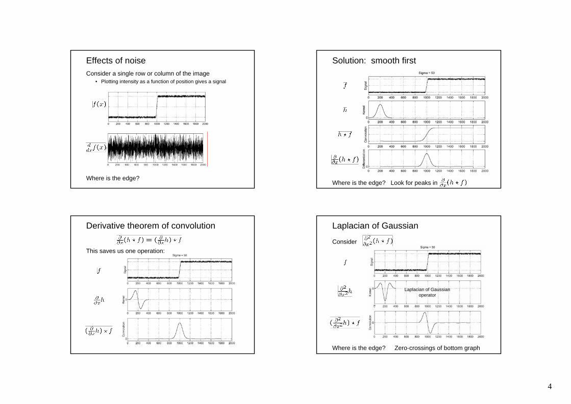
Derivative theorem of convolution
This saves us one operation:
Laplacian of Gaussian
Consider
Laplacian of Gaussianoperator
Where is the edge? Zero-crossings of bottom graph
5
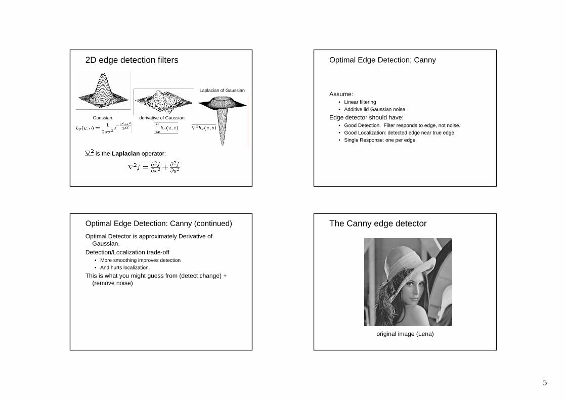
2D edge detection filters
is the Laplacian operator:
Laplacian of Gaussian
Gaussian derivative of Gaussian
Optimal Edge Detection: Canny
Assume: • Linear filtering• Additive iid Gaussian noise
Edge detector should have:• Good Detection. Filter responds to edge, not noise.• Good Localization: detected edge near true edge.• Single Response: one per edge.
Optimal Edge Detection: Canny (continued)Optimal Detector is approximately Derivative of
Gaussian.Detection/Localization trade-off
• More smoothing improves detection• And hurts localization.
This is what you might guess from (detect change) + (remove noise)
The Canny edge detector
original image (Lena)
6
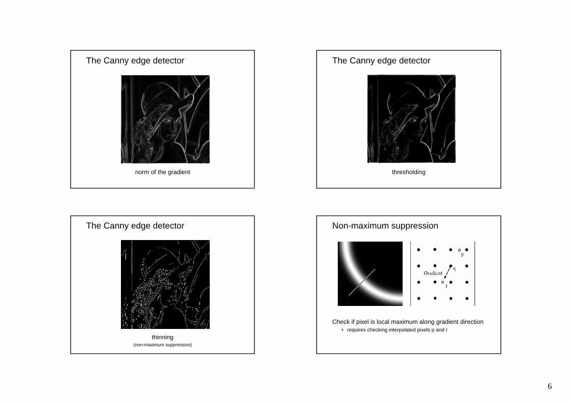
The Canny edge detector
norm of the gradient
The Canny edge detector
thresholding
The Canny edge detector
thinning(non-maximum suppression)
Non-maximum suppression
Check if pixel is local maximum along gradient direction• requires checking interpolated pixels p and r
7
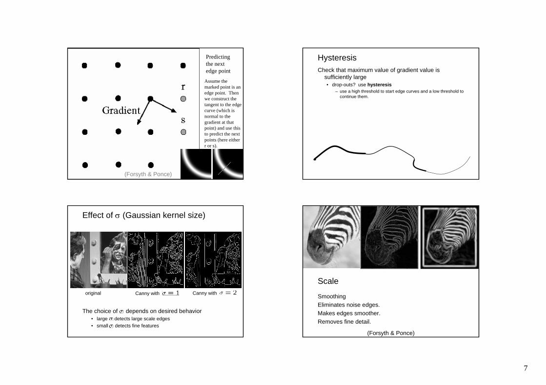
Predictingthe nextedge point
Assume the marked point is an edge point. Then we construct the tangent to the edge curve (which is normal to the gradient at that point) and use this to predict the next points (here either r or s).
(Forsyth & Ponce)
HysteresisCheck that maximum value of gradient value is
sufficiently large• drop-outs? use hysteresis
– use a high threshold to start edge curves and a low threshold tocontinue them.
Effect of σ (Gaussian kernel size)
Canny with Canny with original
The choice of depends on desired behavior• large detects large scale edges• small detects fine features
(Forsyth & Ponce)
Scale
SmoothingEliminates noise edges.Makes edges smoother.Removes fine detail.

8
fine scalehigh threshold
coarse scale,high threshold
coarsescalelowthreshold
9
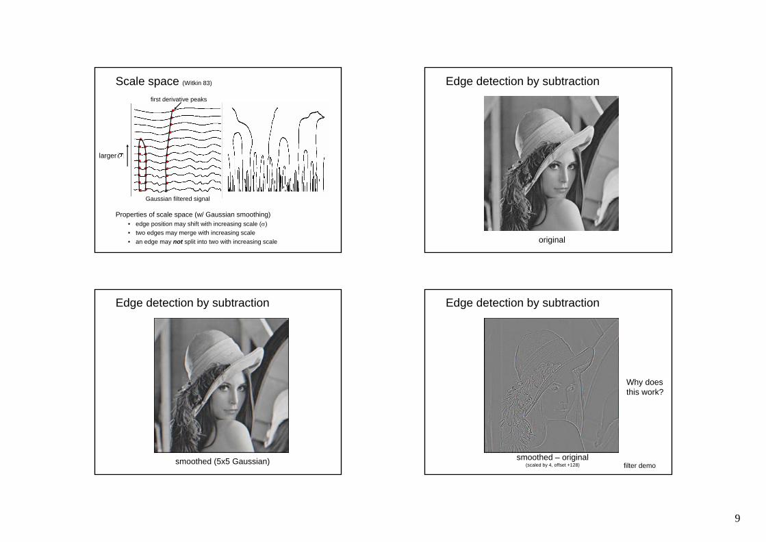
Scale space (Witkin 83)
Properties of scale space (w/ Gaussian smoothing)• edge position may shift with increasing scale (σ)• two edges may merge with increasing scale • an edge may not split into two with increasing scale
larger
Gaussian filtered signal
first derivative peaks
Edge detection by subtraction
original
Edge detection by subtraction
smoothed (5x5 Gaussian)
Edge detection by subtraction
smoothed – original(scaled by 4, offset +128)
Why doesthis work?
filter demo
10
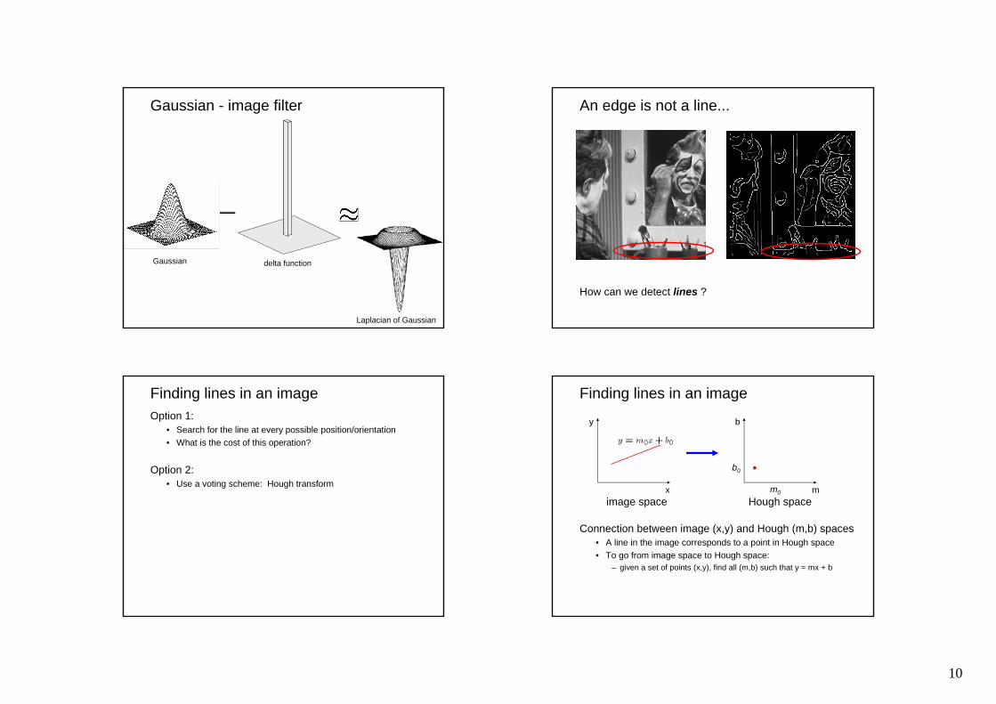
Gaussian - image filter
Laplacian of Gaussian
Gaussian delta function
An edge is not a line...
How can we detect lines ?
Finding lines in an imageOption 1:
• Search for the line at every possible position/orientation• What is the cost of this operation?
Option 2:• Use a voting scheme: Hough transform
Finding lines in an image
Connection between image (x,y) and Hough (m,b) spaces• A line in the image corresponds to a point in Hough space• To go from image space to Hough space:
– given a set of points (x,y), find all (m,b) such that y = mx + b
x
y
m
b
m0
b0
image space Hough space

11
Finding lines in an image
Connection between image (x,y) and Hough (m,b) spaces• A line in the image corresponds to a point in Hough space• To go from image space to Hough space:
– given a set of points (x,y), find all (m,b) such that y = mx + b• What does a point (x0, y0) in the image space map to?
x
y
m
b
image space Hough space
– A: the solutions of b = -x0m + y0
– this is a line in Hough space
x0
y0
Hough transform algorithmTypically use a different parameterization
• d is the perpendicular distance from the line to the origin• θ is the angle this perpendicular makes with the x axis• Why?
Hough transform algorithmTypically use a different parameterization
• d is the perpendicular distance from the line to the origin• θ is the angle this perpendicular makes with the x axis• Why?
Basic Hough transform algorithm1. Initialize H[d, θ]=02. for each edge point I[x,y] in the image
for θ = 0 to 180
H[d, θ] += 13. Find the value(s) of (d, θ) where H[d, θ] is maximum4. The detected line in the image is given by
What’s the running time (measured in # votes)?
ExtensionsExtension 1: Use the image gradient
1. same2. for each edge point I[x,y] in the image
compute unique (d, θ) based on image gradient at (x,y)H[d, θ] += 1
3. same4. same
What’s the running time measured in votes?
Extension 2• give more votes for stronger edges
Extension 3• change the sampling of (d, θ) to give more/less resolution
Extension 4• The same procedure can be used with circles, squares, or any
other shape

12
ExtensionsExtension 1: Use the image gradient
1. same2. for each edge point I[x,y] in the image
compute unique (d, θ) based on image gradient at (x,y)H[d, θ] += 1
3. same4. same
What’s the running time measured in votes?
Extension 2• give more votes for stronger edges
Extension 3• change the sampling of (d, θ) to give more/less resolution
Extension 4• The same procedure can be used with circles, squares, or any
other shape
Hough demos
Line : http://www/dai.ed.ac.uk/HIPR2/houghdemo.htmlhttp://www.dis.uniroma1.it/~iocchi/slides/icra2001/java/hough.html
Circle : http://www.markschulze.net/java/hough/
Hough Transform for CurvesThe H.T. can be generalized to detect any curve that
can be expressed in parametric form:• Y = f(x, a1,a2,…ap)• a1, a2, … ap are the parameters• The parameter space is p-dimensional• The accumulating array is LARGE!
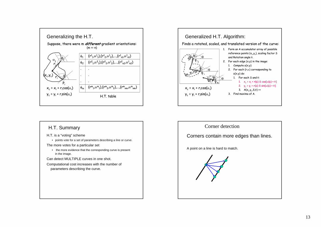
Generalizing the H.T.The H.T. can be used even if the curve has not a The H.T. can be used even if the curve has not a simple analytic form!simple analytic form!
1.1. Pick a reference point (Pick a reference point (xxcc,y,ycc))2.2. For i = 1,…,n :For i = 1,…,n :
1.1. Draw segment to PDraw segment to Pii on the boundary.on the boundary.2.2. Measure its length Measure its length rrii, and its , and its
orientation orientation ααii..3.3. Write the coordinates of (Write the coordinates of (xxcc,y,ycc) as a ) as a
function of function of rrii and and ααii4.4. Record the gradient orientation Record the gradient orientation φφii at Pat Pi.i.
3.3. Build a table with the data, indexed by Build a table with the data, indexed by φφii ..
((xxcc,y,ycc))
φφiirrii
PPii
ααii
xxcc = x= xii + + rriicos(cos(ααii))
yycc = = yyii + + rriisin(sin(ααii))
13
Generalizing the H.T.
((xxcc,y,ycc))
PPii
φφiirrii ααii
xxcc = x= xii + + rriicos(cos(ααii))
yycc = = yyii + + rriisin(sin(ααii))
Suppose, there were m Suppose, there were m differentdifferent gradient orientations:gradient orientations:(m <= n)(m <= n)
φφ11
φφ22
..
..
..
φφmm
(r(r1111,,αα11
11),(r),(r1122,,αα11
22),…,(r),…,(r11n1n1,,αα11
n1n1))
(r(r2211,,αα22
11),(r),(r2222,,αα11
22),…,(r),…,(r22n2n2,,αα11
n2n2))
..
..
..
(r(rmm11,,ααmm
11),(r),(rmm22,,ααmm
22),…,(),…,(rrmmnmnm,,ααmm
nmnm))
φφjj
rrjj
ααjj
H.T. tableH.T. table
Generalized H.T. Algorithm:
xxcc = x= xii + + rriicos(cos(ααii))
yycc = = yyii + + rriisin(sin(ααii))
Finds a rotated, scaled, and translated version of the curve:Finds a rotated, scaled, and translated version of the curve:
((xx cc,y,y cc)) PP ii
φφ iiSrSr ii αα ii θθ
PP jj
φφ jjSrSr jjαα jj θθ
PP kk
φφ iiSrSr kkαα kk θθ
1.1. Form an A accumulator array of possible Form an A accumulator array of possible reference points (reference points (xxcc,y,ycc), scaling factor S ), scaling factor S and Rotation angle and Rotation angle θθ..
2.2. For each edge (x,y) in the image:For each edge (x,y) in the image:1.1. Compute Compute φφ(x,y)(x,y)2.2. For each (r,For each (r,αα) corresponding to ) corresponding to
φφ(x,y) do:(x,y) do:1.1. For each S and For each S and θθ::
1.1. xxcc = x= xii + r(+ r(φφ) S ) S cos[cos[αα((φφ) + ) + θθ]]2.2. yycc = = yyii + r(+ r(φφ) S sin[) S sin[αα((φφ) + ) + θθ]]3.3. A(xA(xcc,y,ycc,S,,S,θθ) ++) ++
3.3. Find maxima of A.Find maxima of A.
H.T. SummaryH.T. is a “voting” scheme
• points vote for a set of parameters describing a line or curve.
The more votes for a particular set• the more evidence that the corresponding curve is present
in the image.
Can detect MULTIPLE curves in one shot.Computational cost increases with the number of
parameters describing the curve.
Corners contain more edges than lines.
A point on a line is hard to match.
Corner detection

14
Corners contain more edges than lines.A corner is easier
Edge Detectors Tend to Fail at Corners
Finding Corners
Intuition:
• Right at corner, gradient is ill defined.
• Near corner, gradient has two different values.
Formula for Finding Corners
⎥⎥⎦
⎤
⎢⎢⎣
⎡=
∑∑∑∑
2
2
yyx
yxx
IIIIII
C
We look at matrix:
Sum over a small region, the hypothetical corner
Gradient with respect to x, times gradient with respect to y
Matrix is symmetric WHY THIS?
15
⎥⎦
⎤⎢⎣
⎡=
⎥⎥⎦
⎤
⎢⎢⎣
⎡=
∑∑∑∑
2
12
2
00λ
λ
yyx
yxx
IIIIII
C
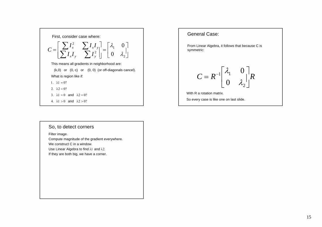
First, consider case where:
This means all gradients in neighborhood are:
(k,0) or (0, c) or (0, 0) (or off-diagonals cancel).
What is region like if:
1. λ1 = 0?
2. λ2 = 0?
3. λ1 = 0 and λ2 = 0?
4. λ1 > 0 and λ2 > 0?
General Case:
From Linear Algebra, it follows that because C is symmetric:
RRC ⎥⎦
⎤⎢⎣
⎡= −
2
11
00λ
λ
With R a rotation matrix.
So every case is like one on last slide.
So, to detect cornersFilter image.Compute magnitude of the gradient everywhere.We construct C in a window.Use Linear Algebra to find λ1 and λ2.If they are both big, we have a corner.